1. Introduction
Against the backdrop of the ongoing global transition of energy systems toward clean and low-carbon paradigms, wind power has become one of the most promising renewable energy sources and is playing an increasingly important role in modern power systems [
1]. With the continuous expansion of installed wind power capacity and grid-connection penetration, wind power has contributed substantially to optimizing the energy structure and reducing dependence on fossil fuels [
2]. However, wind power output is characterized by pronounced volatility, intermittency, and uncertainty, which imposes more stringent requirements on power system dispatch optimization, reserve allocation, and renewable energy accommodation under large-scale grid integration [
3]. Therefore, developing wind power forecasting models with high accuracy and strong robustness has become a critical foundation for ensuring the secure and stable operation of power systems and supporting the integration of high-penetration renewable energy [
4]. From a sustainability perspective, improving wind power forecasting can reduce renewable-energy curtailment, support low-carbon dispatch, and enhance the operational resilience of power systems with high renewable penetration.
Compared with conventional load profiles, wind power output is simultaneously influenced by a multitude of factors, including wind speed, wind direction, meteorological perturbations, and turbine operational states, thereby exhibiting pronounced non-linearity, non-stationarity, and multi-scale dynamics [
4]. In multi-step-ahead forecasting scenarios, models must not only characterize rapid local fluctuations but also capture trend evolution over extended horizons. Meanwhile, as the forecasting horizon increases, cumulative error propagation further undermines the stability of medium- and long-term predictions. Consequently, how to simultaneously address trend modeling, local dynamics characterization, and multi-step error mitigation within a unified framework remains a critical challenge in wind power forecasting [
5].
To address this task, previous research has successively developed statistical, conventional machine learning, and deep learning models. Statistical methods, such as the Auto-Regressive Integrated Moving Average (ARIMA) model, possess solid theoretical foundations for processing linear or weakly stationary sequences [
6]. However, they often require extensive feature engineering or preprocessing when dealing with the strong non-linearity and non-stationarity inherent in wind power output. Subsequently, Recurrent Neural Networks (RNNs), Long Short-Term Memory (LSTM) networks [
7], and Gated Recurrent Units (GRUs) [
8] have been widely applied to wind power and related time-series forecasting tasks. Although effective in modeling local dependencies, these methods still suffer from insufficient capture of long-range dependencies and information attenuation over long historical horizons. In recent years, attention-based Transformer variants have offered promising alternatives for long-sequence forecasting [
9]. Specifically, Informer reduces computational complexity via ProbSparse self-attention [
10]; Autoformer integrates sequence decomposition with an autocorrelation mechanism to enhance trend and periodicity modeling [
11]; and Reformer [
12], PatchTST [
13], and TimesNet [
14] enhance long-sequence forecasting performance through efficient attention mechanisms, patch-level representations, and 2D temporal variation modeling, respectively. Nonetheless, the literature also indicates that Transformers do not consistently outperform simpler baseline models in scenarios characterized by intense noise, limited sample sizes, or pronounced local fluctuations [
15]. For complex sequences like wind power output, where trends, periodicities, and perturbations are highly coupled, there remains significant scope for exploration on how to simultaneously enhance long-range dependency modeling and local dynamic feature extraction.
To alleviate the difficulty of directly modeling non-stationary sequences, sequence decomposition paradigms have been widely integrated into time-series forecasting models in recent years. The core concept involves explicitly or implicitly decoupling the smooth trend from high-frequency fluctuations within the raw sequence, thereby providing structured representations that are easier to model for downstream forecasting networks. Related studies typically employ techniques such as Empirical Mode Decomposition (EMD) [
16], Variational Mode Decomposition (VMD) [
17], or Wavelet Transform (WT) [
18] to decompose the original sequence into various frequency components for individual modeling. Although these approaches mitigate modeling difficulty to a certain extent [
19], performing offline decomposition on the entire sequence prior to the train–test split introduces a latent risk of future information leakage, thereby compromising the consistency between offline evaluation and online deployment. On the other hand, while current hybrid models attempt to combine long-range dependency and local modeling pathways, they often resort to static fusion strategies during the feature integration stage, such as concatenation, linear summation, or fixed weighting. These static methods fail to adaptively adjust the contribution ratios of different pathways in response to dynamic variations in the input states, which limits the utilization efficiency of complementary information and impairs model interpretability [
20].
Furthermore, error correction in existing multi-step forecasting models is predominantly executed in the time domain, leaving the potential spectral structures within the predicted outputs underutilized [
21]. In fact, wind power series typically exhibit a coexistence of trend variations, periodic fluctuations, and local oscillations. Relying solely on time-domain fitting often fails to fully reconstruct these multi-scale structures; this issue becomes more pronounced under long forecasting horizons, where periodic drifts and oscillatory distortions are highly prone to accumulation. Consequently, incorporating frequency-domain residual compensation on top of time-domain predictions holds significant promise for enhancing the model’s capability to reconstruct periodic components and local oscillatory patterns.
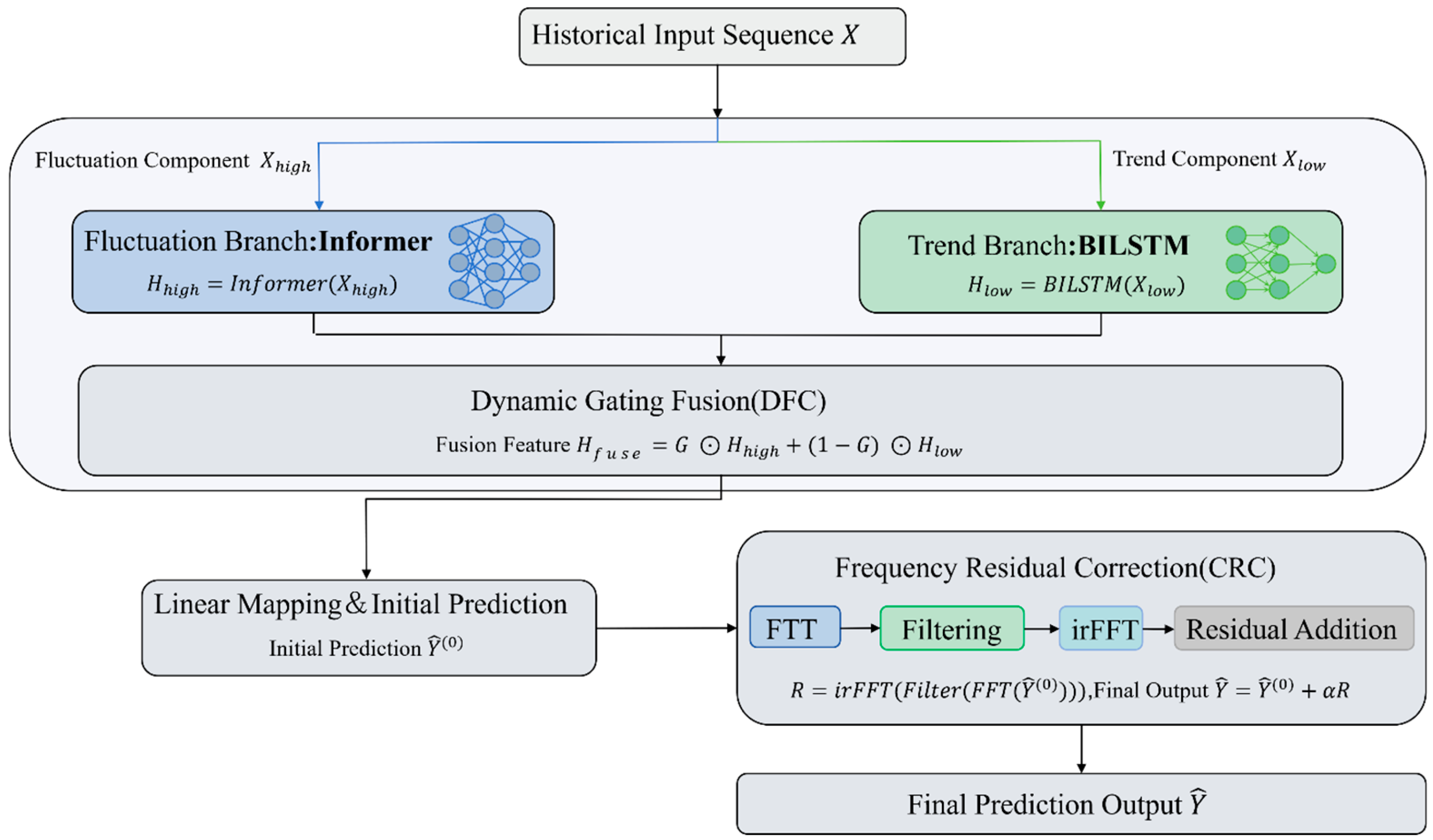
Based on the foregoing analysis, this study proposes a wind power forecasting model that integrates embedded sequence decomposition, a Dynamic Fusion Component, and frequency-domain residual correction, termed CoFFormer. The model first performs a lightweight trend–fluctuation decomposition within the network, together with a historical truncation and future placeholder design, to minimize potential future-information interference during the forecasting process. Subsequently, heterogeneous temporal representations are learned through an attention-based fluctuation branch for long-range dependency modeling and a recurrent-structure-based trend branch for trend evolution modeling, while a dynamic gated fusion mechanism is employed to realize input-dependent adaptive feature collaboration. Finally, a frequency-domain residual correction module is introduced at the prediction output stage to conduct spectral mapping and residual refinement on the preliminary forecasts, thereby enhancing the model’s ability to recover periodic structures and local oscillatory components.
The main contributions are summarized as follows:
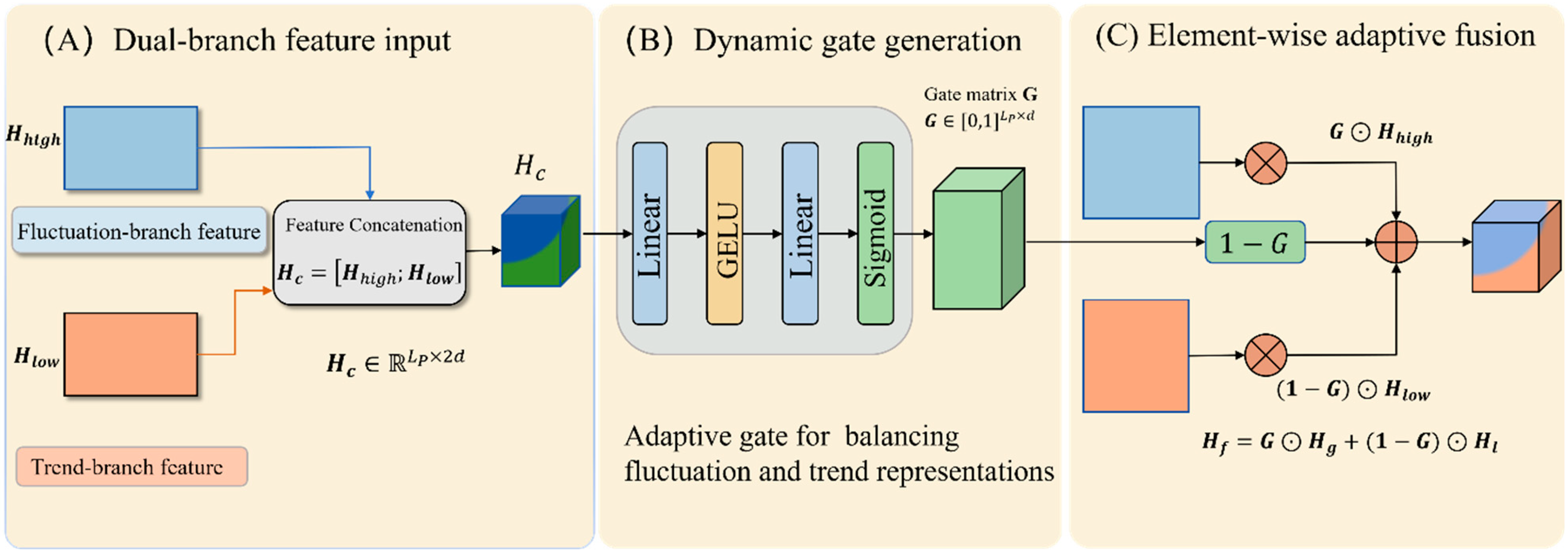
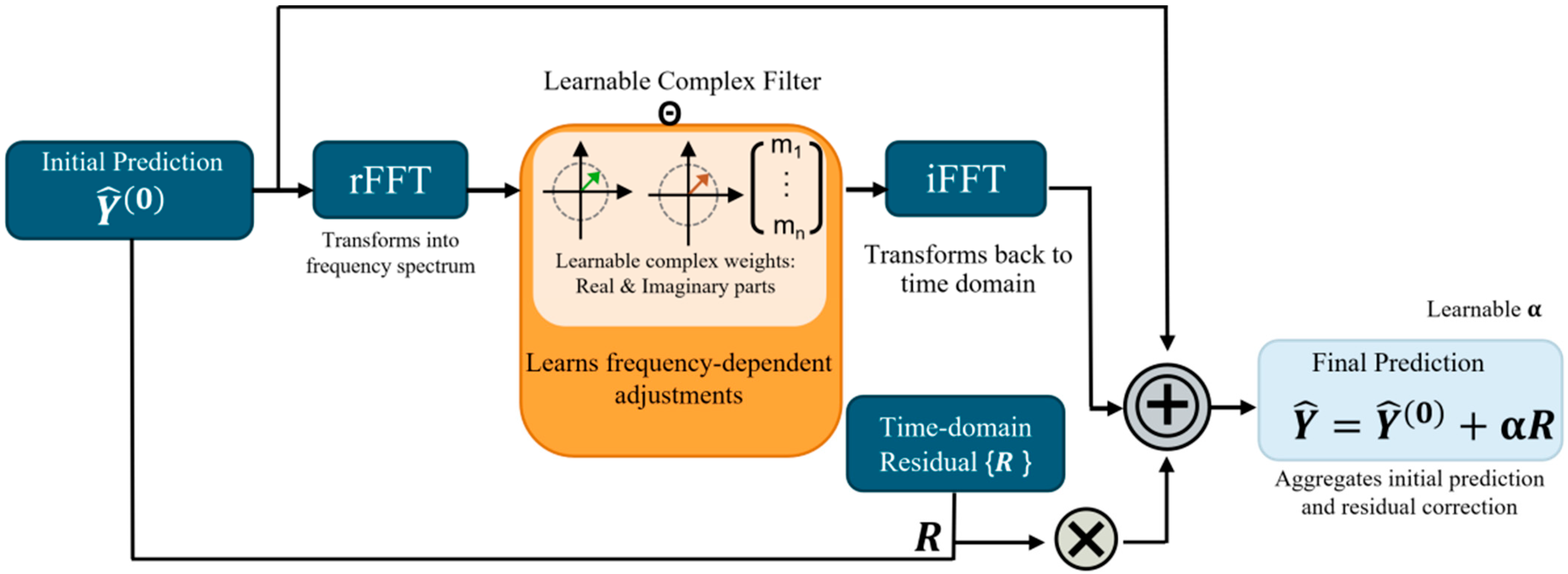
(1) An embedded sequence decomposition (SD) and dual-path collaborative modeling framework is developed to perform trend–fluctuation decoupling inside the forecasting network. This design reduces the mismatch between offline decomposition and online forecasting, thereby improving consistency with practical deployment scenarios. (2) A Dynamic Fusion Component (DFC) is introduced to learn input-dependent weights for long-range fluctuation representations and trend-evolution representations. Unlike static concatenation or fixed-weight fusion, DFC adaptively coordinates heterogeneous temporal features and enables interpretable analysis through gate-weight visualization. (3) A Frequency-domain Correction via Residual Compensation (CRC) module is proposed to refine preliminary time-domain forecasts in the spectral domain. This output-side correction compensates for periodic deviations and local oscillatory distortions, thereby improving the stability of multi-step forecasting.
4. Experiments
To verify the effectiveness of the proposed CoFFormer for non-stationary time-series forecasting, experiments are conducted on four public datasets. The proposed model is evaluated and analyzed from multiple perspectives, including overall forecasting performance, ablation studies, performance under different forecasting horizons, and model interpretability.
4.1. Experimental Setup
4.1.1. Dataset Description
To evaluate the performance of the proposed model, four public datasets are utilized in this study: ETTh2 [
10], wind_speed [
30], WindPower [
31], and Location [
32]. Specifically, wind_speed, WindPower, and Location2 are core benchmarks in the wind energy domain, which serve to test the forecasting accuracy of the model under scenarios characterized by strong wind–meteorological perturbations. In addition, to validate the cross-domain generalization capability of the proposed model regarding non-stationary features, the ETTh2 dataset—a standard benchmark in long-term time-series forecasting—is further introduced. Within the Electricity Transformer Temperature (ETT) series, ETTh2 exhibits more pronounced non-stationary evolution and local fluctuations, which closely align with the statistical characteristics of wind power. Consequently, it is selected as a representative benchmark for cross-domain generalization evaluation. The key statistics of these datasets are summarized in
Table 1.
4.1.2. Evaluation Metrics
Mean Squared Error (MSE) and Mean Absolute Error (MAE) are adopted as the evaluation metrics, which are defined as follows:
Here,
and
denote the ground-truth value and the predicted value, respectively, and
denotes the number of test samples. MSE and MAE are used as primary metrics because they measure squared and absolute errors without division by the target value. MAPE and sMAPE are not used for the main comparison because normalized target values can approach zero, making percentage errors unstable. Peak relative error also depends strongly on the peak threshold. To address extreme variations,
Section 4.3.3 reports Ramp-MAE, Ramp-RMSE, Ramp Magnitude Error, and Direction Accuracy.
4.1.3. Baselines
Six representative time-series forecasting models are selected as baselines, including one recurrent neural network model and five Transformer-based or advanced deep forecasting models: BiLSTM [
25], Informer [
10], Reformer [
12], Autoformer [
11], PatchTST [
13], and TimesNet [
14]. BiLSTM is used as a classical recurrent baseline, while Informer and Reformer represent efficient Transformer variants for long-sequence forecasting. Autoformer is adopted as a decomposition-based forecasting model, and PatchTST and TimesNet are included due to their strong performance in recent long-term time-series forecasting tasks. The proposed CoFFormer is compared with these baselines under the same data partition, input length, forecasting horizon, and evaluation metrics. For publicly available models, the recommended settings in the original papers are followed when possible, with minor adjustments based on the validation set.
4.1.4. Parameter Settings and Training Details
All experiments were implemented within the PyTorch (version 2.7.0) deep learning framework [
33] and executed on a single NVIDIA RTX 5060 GPU. During sequence sample construction, the historical input length was fixed at 96 time steps, while the decoder guidance label length was set to 48. To comprehensively evaluate the forecasting capability of the model across different temporal scales, the prediction horizon set was defined as {1, 3, 12, 24, 48, 96}. This setting implies that the model leverages historical wind-condition states over a relatively stable long-period interval to progressively infer the evolution trend of wind power from ultra-short-term to medium- and long-term horizons.
During network training, a joint optimization strategy combining the primary loss and auxiliary loss was adopted as the objective function, with the aim of simultaneously ensuring accurate fitting of the overall trend and correction of local dynamic residuals. The Adam optimizer [
34] was employed, with the initial learning rate set to
, the batch size fixed at 32, and the maximum number of training epochs set to 40. To improve convergence quality and effectively mitigate overfitting, the ReduceLROnPlateau learning-rate scheduling strategy was introduced, together with an early stopping mechanism [
35]. In addition, considering that non-stationary wind power series are often accompanied by abrupt local fluctuations, the gradient clipping threshold was set to 5.0. This configuration substantially alleviates the gradient explosion problem induced by complex fluctuation patterns and, while preserving the inference capability of the backbone network, markedly enhances the stability of the multi-horizon training process.
4.2. Overall Forecasting Performance
4.2.1. Comparison with General Forecasting Baselines
To comprehensively evaluate the forecasting performance of the proposed CoFFormer, comparative experiments against baseline models were conducted across four datasets. The multi-step forecasting results are summarized in
Table 2, where the best and second-best results are highlighted in bold and underlined, respectively.
Overall, CoFFormer demonstrates strong competitiveness across all four datasets under multiple forecasting-horizon settings and achieves the best or near-best performance in a variety of short- to medium-term and medium- to long-term forecasting scenarios. These results indicate that the proposed model is well capable of capturing trend variations, local perturbations, and multi-scale fluctuation patterns in non-stationary time-series forecasting.
On the ETTh2 dataset, CoFFormer achieves MSE values of 0.0202, 0.0957, and 0.1508 at forecasting horizons of 3, 12, and 24 steps, respectively. Its overall performance surpasses that of most benchmark models, indicating that the proposed model possesses strong capability in modeling the coupled characteristics of underlying trends and fluctuations. Although its performance at longer forecasting horizons is slightly inferior to that of PatchTST and TimesNet, it still substantially outperforms Informer, Reformer, and Autoformer, thereby demonstrating favorable robustness and stability.
On the wind_speed dataset, CoFFormer attains the lowest MSE values at forecasting horizons of 3 and 48 steps, reaching 0.3201 and 0.7357, respectively, while maintaining competitive performance at the 96-step forecasting horizon. These results indicate that the proposed model also exhibits strong adaptability to meteorological time series characterized by pronounced stochasticity and significant local fluctuations. On the WindPower and Location2 datasets, CoFFormer also demonstrates strong generalization capability. Specifically, on the WindPower dataset, the model achieves the lowest MSE of 0.0617 at the 3-step forecasting horizon and outperforms most baselines at the 48-step forecasting horizon. On the Location2 dataset, the model attains near-optimal performance for 1-step forecasting and achieves the lowest MAE at the 48-step forecasting horizon. Although certain competing models exhibit slight advantages on individual metrics at specific forecasting horizons, CoFFormer delivers a more balanced overall performance across different datasets and forecasting ranges.
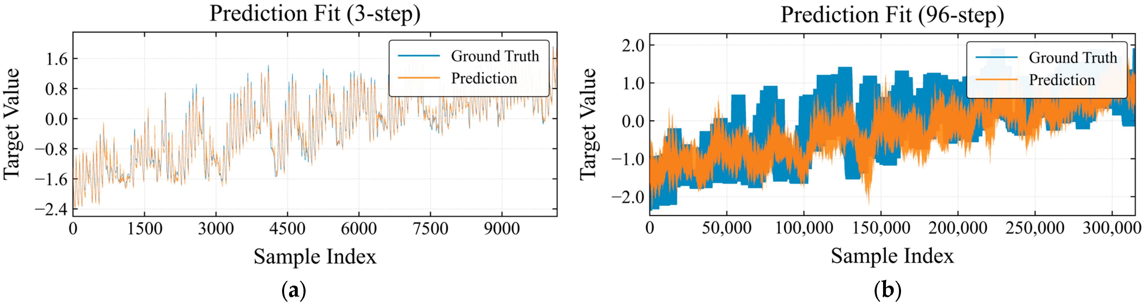
To further validate the fitting capability of the proposed model at the sample level, two representative sample segments from the ETTh2 test set are selected for visual comparison, as illustrated in
Figure 4. These two samples exhibit pronounced local fluctuations, stage-wise variations, and trend changes, thereby providing a representative basis for assessing forecasting performance under complex non-stationary scenarios.
As can be observed from
Figure 4, CoFFormer is able to effectively track the overall variation trend of the ground-truth series in both sample segments, while maintaining relatively stable forecasting results in intervals with frequent fluctuations. For local peaks and troughs, as well as continuously oscillatory intervals, the model still exhibits certain deviations; however, the overall predicted trajectory remains highly consistent with the true values, without showing evident systematic drift or excessive smoothing.
Taken together, the results in
Table 2 and
Figure 4 suggest that CoFFormer achieves favorable forecasting accuracy and stability across multiple datasets and forecasting horizons, while also demonstrating strong capability in fitting real-world time series. The effectiveness of CoFFormer is further examined through external-baseline comparisons, ablation studies, and mechanism analyses.
4.2.2. Comparison with an External Decomposition-Based Baseline
To evaluate the benefit of embedded decomposition over a conventional decomposition-then-forecasting pipeline, CoFFormer is compared with VMD-BiLSTM-Informer on ETTh2 and WindPower under the 24- and 96-step settings, using the same data partitions, input length, and evaluation metrics.
As shown in
Table 3, CoFFormer outperforms VMD-BiLSTM-Informer in five of the eight metric-horizon cases and is nearly tied in ETTh2 MAE at 24 steps. For ETTh2 at 96 steps, CoFFormer reduces MSE/MAE by 15.10%/5.63%. For WindPower at 96 steps, CoFFormer lowers MAE by 8.20% but yields a higher MSE, suggesting better average tracking but sensitivity to a few large deviations. Therefore, the benefit of embedded decomposition should be interpreted as a robust but not universal gain, especially when end-to-end feature fusion and residual correction are effective.
4.2.3. Statistical Significance Analysis
To assess the statistical reliability of the differences reported in
Table 2, paired block sign-flip tests with Holm correction were conducted on ETTh2 and WindPower under the 24- and 96-step settings.
As shown in
Table 4, six of the 32 comparisons are statistically significant, five of which favor CoFFormer, mainly at the 24-step horizon. This pattern is consistent with the coordinated effects of embedded decomposition, dynamic feature collaboration, and frequency-domain residual compensation, which provide more stable gains over moderate forecasting horizons. At the 96-step horizon, most differences are not significant, indicating increasing performance convergence among strong models as forecasting uncertainty accumulates. TimesNet is significantly better only in MAE on ETTh2 at 96 steps, possibly because its multi-period representation is better suited to the long-cycle characteristics of this dataset. Overall, CoFFormer achieves reliable advantages in selected settings while remaining competitive in the others.
4.3. Ablation and Component-Specific Analysis
4.3.1. Component Ablation
To systematically evaluate the contribution of each constituent module to the forecasting performance of the model, ablation experiments were conducted on the ETTh2 and WindPower datasets. Comparative analyses were further performed for the 24-step and 96-step forecasting horizons to validate the effectiveness of each module and its synergistic gains. The detailed ablation settings are presented in
Table 5 and
Table 6, respectively.
Table 5 and
Table 6 present the ablation results of the model on the ETTh2 and WindPower datasets. Overall, the complete CoFFormer achieves the lowest MSE and MAE in both the 24-step and 96-step forecasting tasks, consistently outperforming all ablated variants. These results confirm the effectiveness of the three key modules—sequence decomposition (SD), dynamic gated fusion (DFC), and frequency-domain residual correction (CRC)—as well as their synergistic and complementary roles within the unified framework.
Specifically, on the ETTh2 dataset, the removal of any module leads to a significant degradation in forecasting accuracy. The increase in prediction error caused by removing the SD module (w/o SD) indicates that sequence decomposition can effectively decouple the trend component from the fluctuation component, thereby mitigating the interference of non-stationary characteristics in the forecasting process. The performance decline observed after removing the DFC module (w/o DFC) confirms that, compared with a fixed fusion pathway, the dynamic gating mechanism can more adaptively coordinate the long-range dependency representations of the fluctuation component and the evolutionary representations of the trend component. Moreover, the loss in accuracy resulting from the removal of the CRC module (w/o CRC) demonstrates that frequency-domain residual correction is critical for compensating periodic biases and local oscillations that are not sufficiently captured in the time domain. The consistent performance degradation observed under the long-horizon (96-step) forecasting setting further validates the robustness of these modules for long-range modeling.
On the WindPower dataset, which exhibits stronger volatility and more complex environmental disturbances, the complete model still maintains a clear overall advantage. In both short-term and long-horizon forecasting tasks, the full CoFFormer achieves the best overall error performance. This demonstrates that the hierarchical mechanism of “input decoupling–dynamic fusion–frequency-domain correction” constructed by the model is highly effective in adapting to complex dynamic variations induced by abrupt wind speed changes, thereby exhibiting excellent generalization capability and robustness across different forecasting horizons.
4.3.2. Dynamic Fusion Versus Fixed-Gate Fusion
To determine whether the learned dynamic gating can be replaced by its approximate mean value, the DFC is compared with a fixed gate of 0.3 while all other model settings remain unchanged.
As shown in
Table 7, dynamic DFC consistently outperforms the fixed gate across both datasets and forecasting horizons. Compared with the fixed weight of 0.3, DFC reduces MSE/MAE by 1.31%/0.28% and 5.42%/3.10% on ETTh2 under the 24- and 96-step settings, respectively; the corresponding reductions on WindPower are 3.11%/4.38% and 1.02%/6.82%. Although a fixed weight can approximate the average branch preference and therefore remains competitive in relatively stable cases, it cannot capture sample- and feature-dependent variations in the relative importance of trend and fluctuation representations. In contrast, DFC adaptively adjusts their contributions according to the input state, yielding more robust performance when temporal dynamics and forecasting uncertainty vary. These results demonstrate that the effectiveness of DFC arises from its state-dependent adaptation rather than merely from the average magnitude of the learned gates.
4.3.3. Stability and Ramp-Event Analysis of CRC
To further examine whether the Correction via Residual Compensation (CRC) module improves forecasting stability beyond point-wise error reduction, this section compares the model outputs before and after CRC using stability metrics, learned frequency responses, and ramp-event indicators. Specifically, BJE measures boundary-jump error, Mean Max Jump and P95 Jump quantify jump amplitudes, Spike Ratio reflects abnormal spike-like variations, and Roughness characterizes local oscillatory intensity. Lower values indicate more stable predicted trajectories.
As shown in
Table 8, CRC reduces most jump- and smoothness-related indicators across both datasets and forecasting horizons. The improvements are especially evident on ETTh2, where Mean Max Jump, P95 Jump, Spike Ratio, and Roughness are substantially decreased. On WindPower, the reductions are more moderate but consistent, indicating that CRC also stabilizes predictions under highly volatile wind-power conditions. Although BJE slightly increases under the ETTh2 96-step setting, the simultaneous improvement in other stability metrics suggests that CRC mainly acts as an incremental residual stabilizer rather than an aggressive global reshaping operation.
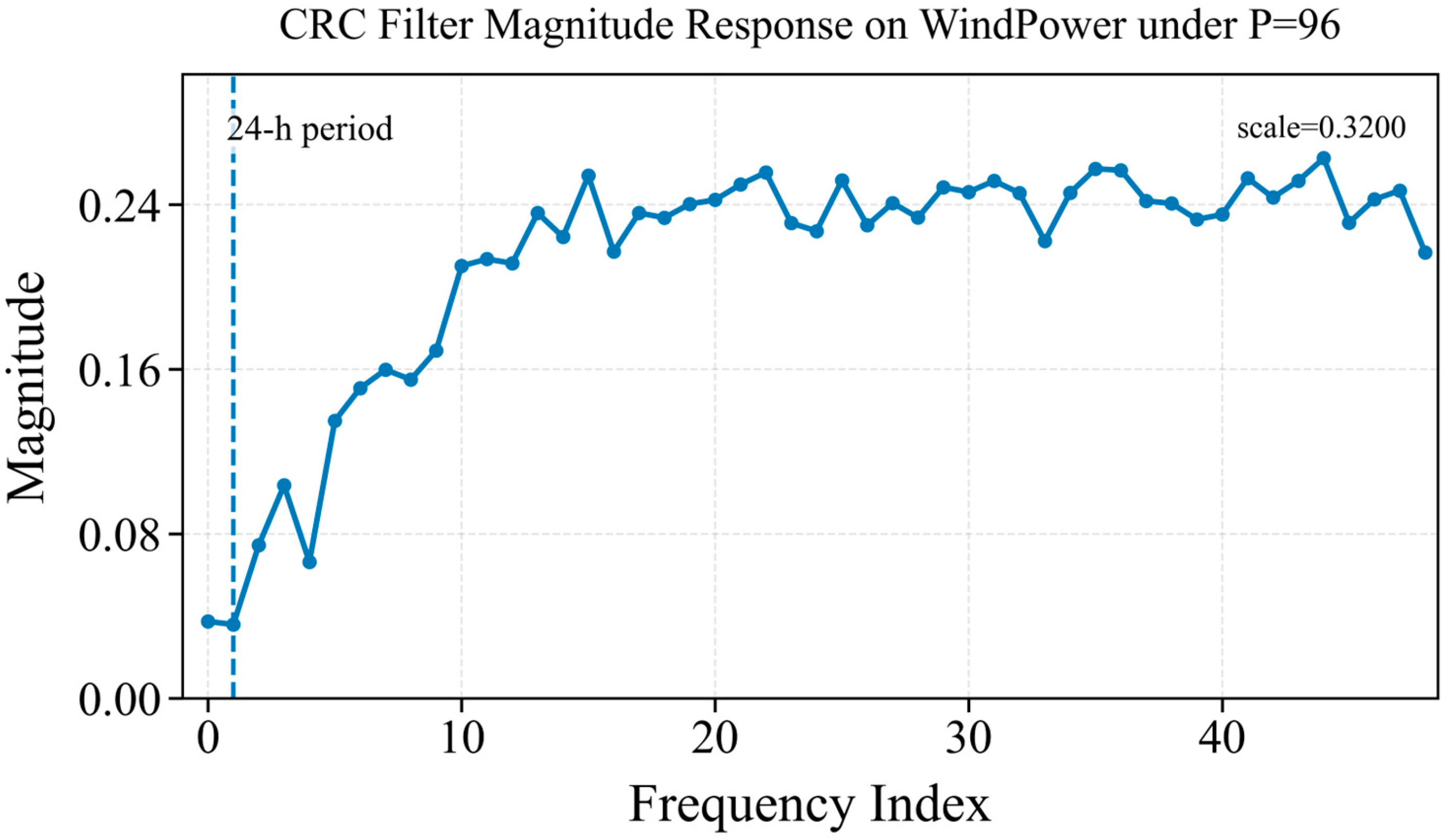
Figure 5 provides a spectral interpretation of the CRC mechanism. The learned filter exhibits non-uniform and non-negligible responses across multiple frequency bins, indicating that CRC adaptively reweights different spectral components rather than applying uniform smoothing or concentrating on a single predefined band. This multi-band modulation supports its role in refining periodic variations and local oscillatory distortions in the preliminary forecasts. Since the frequency bins are not explicitly mapped to physical periods, the result should be interpreted as evidence of adaptive spectral refinement rather than direct verification of a specific physical cycle.
Table 9 further examines CRC under ramp events. CRC slightly reduces Ramp-MAE/RMSE and improves Direction Accuracy at both horizons, while Ramp Magnitude Error changes only marginally. Together with
Table 8, these results indicate that CRC does not introduce evident boundary spikes or spectral-leakage-induced distortion; instead, it provides mild residual stabilization during abrupt wind-power changes.
4.4. Sensitivity to the Moving-Average Window Size
To assess the sensitivity of the embedded decomposition module to the moving-average window size, K was varied on WindPower under the 96-step setting while all other configurations remained unchanged. The candidate values cover narrow, moderate, and wide smoothing scales. Odd-valued windows were used to maintain symmetric temporal alignment and reduce additional moving-average phase displacement.
As shown in
Table 10, the moving-average window directly affects the quality of trend–fluctuation decoupling. Small windows (
and
) provide insufficient smoothing, allowing short-term disturbances to remain in the trend component and weakening the specialization of the dual-path representations. Increasing
to 25 substantially improves both metrics, indicating a more appropriate separation of slowly varying trends and high-frequency fluctuations. Although
achieves a slightly lower MSE, its higher MAE suggests that excessive smoothing may suppress a few large deviations while obscuring moderate local variations. Therefore,
is adopted as the default setting because it provides the lowest MAE with competitive MSE, offering the most balanced input representation for subsequent dual-path modeling and dynamic fusion.
4.5. Performance Analysis Under Different Forecast Horizons
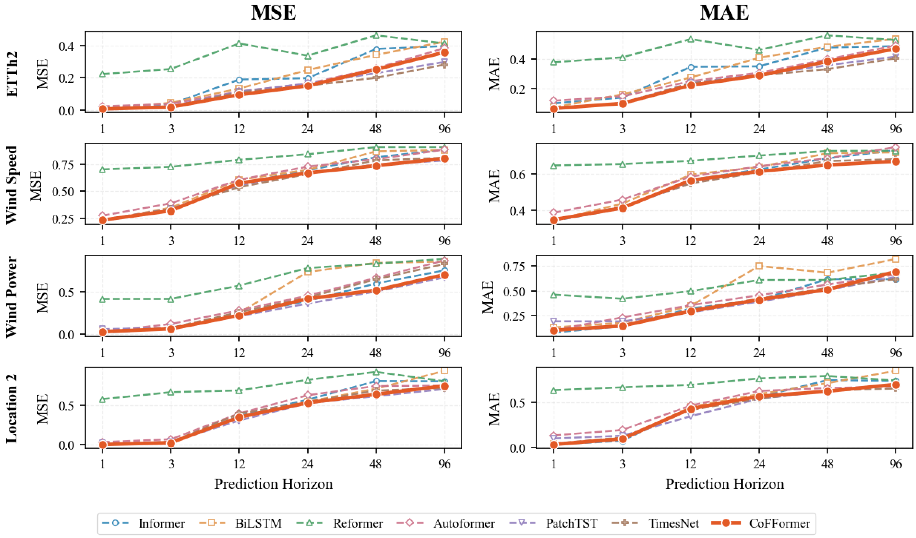
To evaluate the stability of the proposed model across different forecasting horizons, this study further compares the error variation trends of all models under different prediction length settings on each dataset. The results are illustrated in
Figure 6.
As shown in
Figure 6, as the forecasting horizon extends from 1-step to 96-step, the MSE and MAE of all models generally exhibit an increasing trend, and the performance gaps among models gradually widen. This indicates that, in long-horizon forecasting, both error accumulation and the difficulty of modeling non-stationary dynamics increase simultaneously, thereby imposing higher requirements on the cross-horizon stability of forecasting models.
The performance gains of CoFFormer are not uniform across datasets and forecasting horizons, which may be attributed to differences in sequence predictability, stochastic variation, and model inductive biases. On ETTh2, the relatively distinguishable trend and local fluctuations allow embedded decomposition and dynamic fusion to provide clearer benefits under the 12-step and 24-step settings. As the forecasting horizon extends to 48 and 96 steps, accumulated uncertainty becomes more pronounced, and PatchTST and TimesNet become more competitive on several metrics. For the more stochastic wind_speed and Location2 datasets, the benefit of the additional model complexity is relatively limited.
Taken together, the results indicate that the coordinated architecture of embedded decomposition, heterogeneous temporal modeling, dynamic fusion, and frequency-domain refinement helps control error growth but does not eliminate the uncertainty inherent in ultra-long-horizon forecasting. CoFFormer should therefore be regarded as a competitive and comparatively balanced model across datasets and horizons rather than as a uniformly optimal model under every setting.
4.6. Model Interpretability and Mechanism Analysis
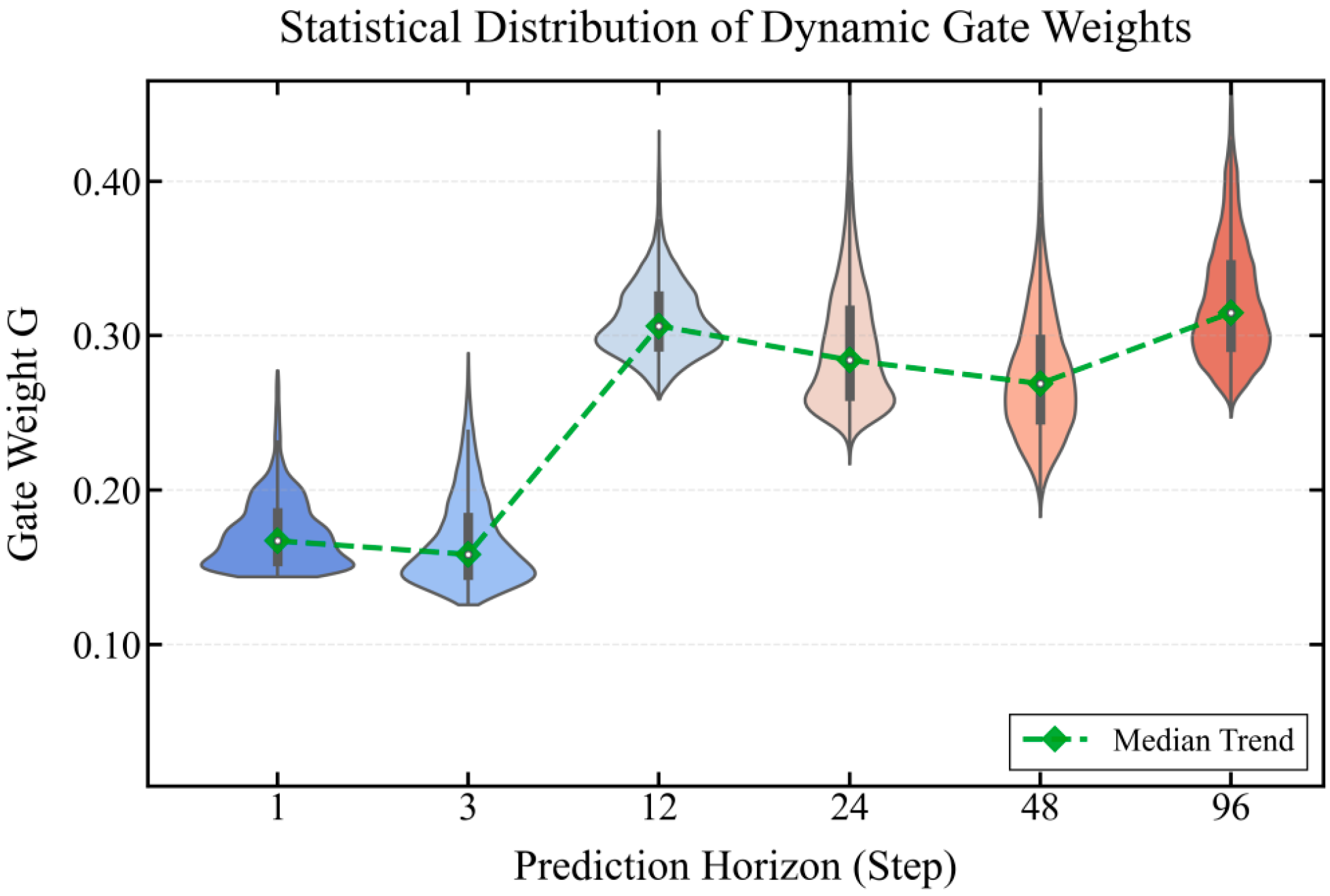
To verify the adaptive coordination capability of the dynamic fusion control (DFC) mechanism for dual-path representations, this study analyzes the distribution of gating weights on the ETTh2 test set under different forecasting horizons and visualizes the results using violin plots, as shown in
Figure 7.
According to the feature fusion design, the gating weight
directly characterizes the relative contribution of the long-range dependency fluctuation representation and the trend-evolution representation to the final fused representation. As shown in
Figure 7, under short-horizon forecasting settings such as 1-step and 3-step, the gating weights are highly concentrated within the range of 0.15–0.20. This indicates that, in short-term forecasting scenarios, the model tends to assign a higher weight to the trend-evolution representation so as to provide more stable short-term sequential evolution information. However, as the forecasting horizon increases from 12-step to 96-step, the median of the gating weight distribution exhibits a pronounced upward trend. This evolution confirms that, in medium- and long-horizon forecasting, the model can adaptively increase the proportion of the long-range dependency fluctuation representation to compensate for the loss of contextual dependency information in long sequences.
Although G remains below 0.5 across all forecasting horizons, this does not mean that DFC can be replaced by a constant trend-dominant weight. The distribution shifts upward and becomes wider as the horizon increases, indicating sample-dependent routing. The fixed-gate experiment in
Table 7 further confirms that dynamic DFC outperforms a fixed weight of 0.3. Thus, the benefit comes from state-dependent adaptation rather than from the average gate magnitude.
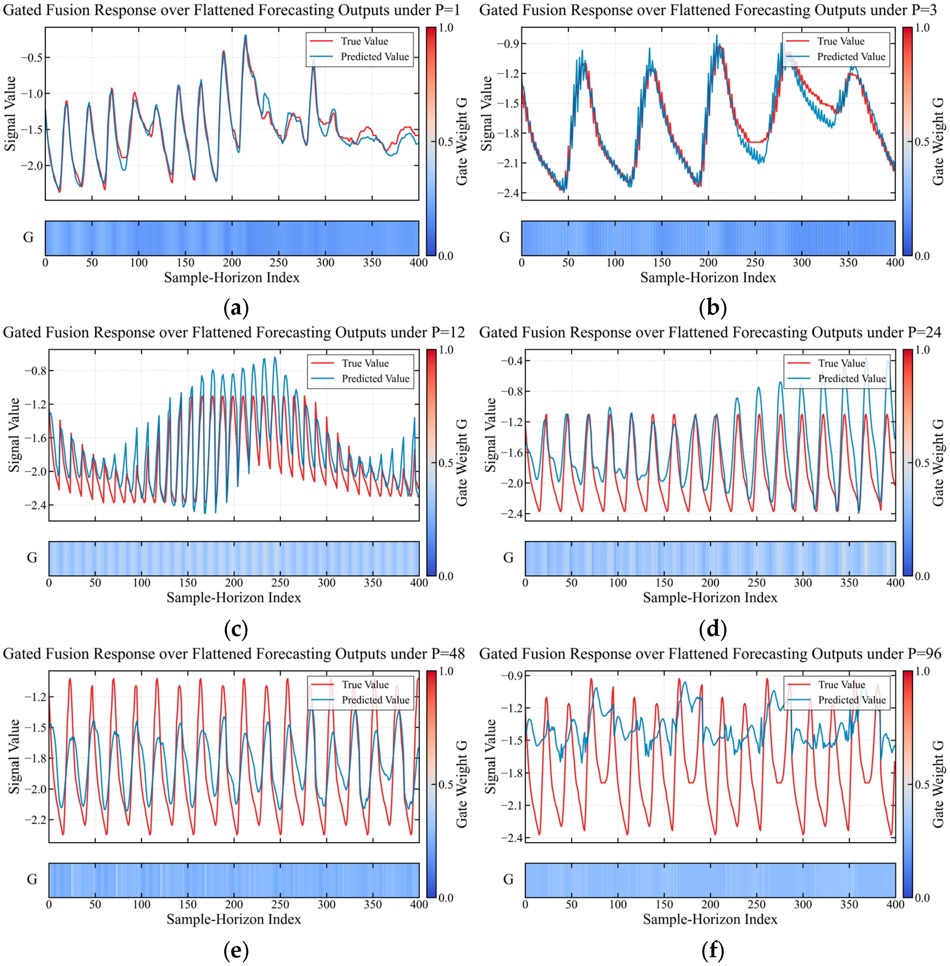
Although the statistical distributions reveal the macroscopic evolution trend of the DFC module, to further examine its microscopic dynamic response along specific forecasting trajectories, this study extracts the continuous time-series responses of the model under different forecasting horizons, as shown in
Figure 8.
As can be directly observed from
Figure 8, the gating weights are not static constants; rather, they are adaptively adjusted with the temporal evolution of the sequence. In short-horizon tasks such as 1-step forecasting, the model output exhibits a high degree of agreement with the ground-truth sequence, and the fluctuations of the gating weights remain relatively stable. Nevertheless, in segments characterized by peak–valley transitions or severe local fluctuations, the gating response still demonstrates sensitive local adaptation, indicating that the model possesses the capability to perceive and respond to abrupt changes in sequence states. As the forecasting horizon extends to 96 steps, the accumulation of prediction errors substantially increases the difficulty of characterizing complex dynamic patterns. Under this more challenging setting, the gating weights not only preserve their time-varying property but also exhibit frequent and pronounced adjustments in specific output segments. This phenomenon, manifested across both global and local scales, fully demonstrates that, for medium- and long-horizon time-series forecasting, the DFC module can continuously and dynamically coordinate the relative contributions of long-range dependency fluctuation representations and trend-evolution representations, thereby maintaining an optimal balance in feature expression across different temporal scales.
4.7. Computational Complexity and Deployment Efficiency Analysis
To further assess the practical deployability of the proposed model, the computational complexity and inference efficiency of CoFFormer are compared with those of representative baseline models under the same experimental setting.
Table 11 shows that CoFFormer provides a balanced trade-off between forecasting capacity and deployment efficiency. Although its cost is higher than that of simple lightweight baselines, this overhead is reasonable because the model integrates embedded decomposition, dual-path modeling, dynamic fusion, and frequency-domain residual correction. Compared with VMD-BiLSTM-Informer, CoFFormer reduces parameters and model size by about 43.2%, while achieving faster inference and higher throughput. It also requires substantially fewer FLOPs than PatchTST and TimesNet. These results suggest that CoFFormer improves structural expressiveness without imposing excessive computational burden.
4.8. Illustration of Forecasting Results for Typical Samples
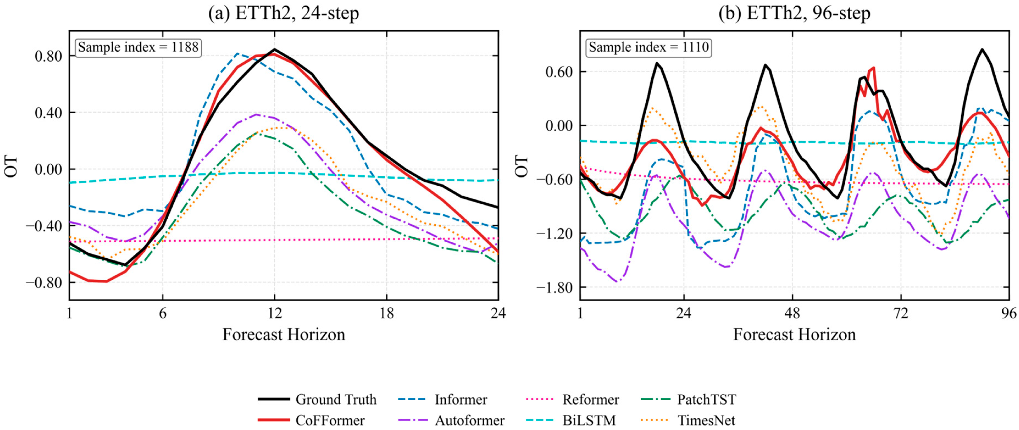
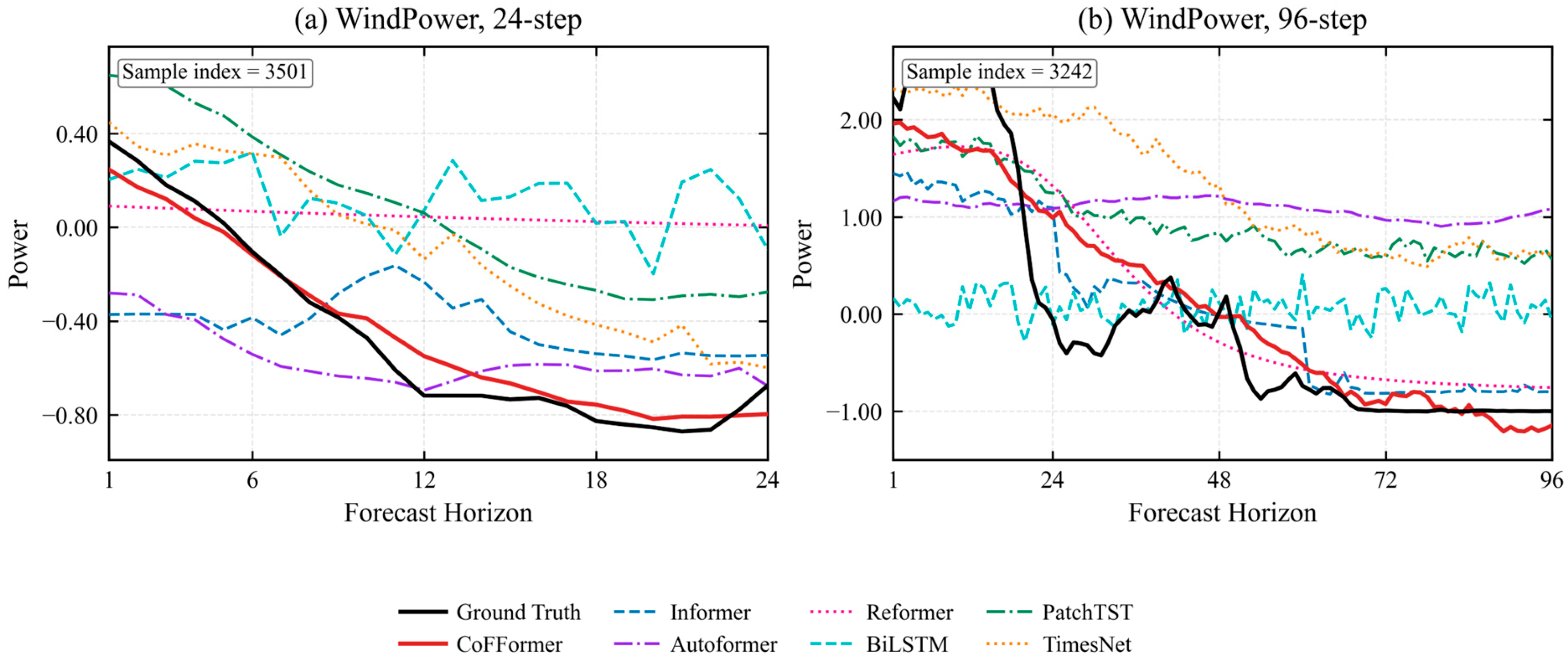
To further provide an intuitive demonstration of the forecasting performance of the models on complex non-stationary time series, this study selects representative sample segments from the test set and visualizes the multi-step forecasting results of different models on the ETTh2 and WindPower datasets, as shown in
Figure 9 and
Figure 10, respectively, including two forecasting horizons, namely 24-step and 96-step.
As can be observed from
Figure 9 and
Figure 10, the forecasting curves produced by CoFFormer closely track the variation patterns of the ground-truth series as a whole, maintaining a high degree of consistency across most rising, declining, and turning intervals, without exhibiting evident systematic drift or excessive smoothing. In particular, in local peak–valley regions and intervals with consecutive fluctuations, the model is still able to accurately recover the amplitude variations and oscillatory patterns of the series, indicating that it not only captures the overall trend evolution but also possesses strong capability in characterizing local dynamics.
This result is highly consistent with the architectural design proposed in this study. First, the embedded sequence decomposition module explicitly decouples the low-frequency trend and high-frequency fluctuation components in the input sequence, thereby reducing the complexity of directly modeling non-stationary series. Second, the dual-path structure composed of Informer and BiLSTM, respectively, strengthens long-range dependency modeling and local dynamic feature extraction, enabling the model to simultaneously respond to global evolution patterns and short-term disturbance variations. Furthermore, the dynamic gated fusion mechanism adaptively adjusts the contributions of the two types of features according to the sample state, alleviating the limitation of static fusion schemes in adapting to different operating conditions. Finally, the frequency-domain residual correction module compensates for periodic biases and local oscillation distortions in the preliminary forecasting results, thereby improving the stability and fine-grained recovery capability of the output curves in multi-step forecasting.
In summary, the visualization results in
Figure 9 and
Figure 10 further demonstrate that CoFFormer can achieve coordinated optimization of trend tracking, fluctuation recovery, and error suppression in complex non-stationary time series, thereby validating the effectiveness of the proposed “input decoupling–heterogeneous modeling–dynamic fusion–frequency-domain correction” framework at the level of representative sample analysis.
4.9. Limitations and Practical Considerations
CoFFormer adopts a rolling-window forecasting scheme in which decomposition is restricted to the observed historical window, ensuring causality with respect to the forecast origin rather than strict pointwise causal filtering. Although the model jointly encodes and dynamically fuses multivariate meteorological and operational information, it remains data-driven, and the learned dependencies should not be interpreted as explicit physical causality. In particular, the influence of air density on the wind-power curve has not been separately modeled or verified. Moreover, the performance gains become less consistent at ultra-long forecasting horizons as uncertainty accumulates. Future work will incorporate derived physical variables, such as air density, introduce physics-informed constraints, and explore more robust long-horizon modeling strategies.
5. Conclusions
This study introduced CoFFormer to address three linked failure modes in multi-step non-stationary forecasting: trend–fluctuation coupling at the input, static weighting of heterogeneous representations, and spectral distortion in preliminary outputs. Its central contribution is the stage-wise coordination of causal embedded decomposition, complementary temporal encoding, state-dependent fusion, and output-side frequency-domain residual correction within one end-to-end pipeline. Across ETTh2, wind_speed, WindPower, and Location2, CoFFormer remained competitive across six horizons, with its clearest advantages at short-to-medium horizons. Removing SD, DFC, or CRC increased both MSE and MAE on ETTh2 and WindPower at 24 and 96 steps; dynamic DFC consistently outperformed a fixed gate, and CRC reduced most jump- and roughness-related indicators. These findings support the proposed coordination mechanism rather than uniform superiority over every baseline. Performance converged with strong competitors at ultra-long horizons, particularly on more stochastic datasets. Future work will incorporate physical priors, spatial dependencies among wind farms, and lighter-weight architectures to improve ultra-long-horizon generalization and deployment efficiency.




 ,
,