Fuzzy Robust Multi-Objective Model for Sustainable and Resilient Supply Chain Network Design Under Disruption Risks and Demand Uncertainty

Abstract

In today’s volatile global environment, designing sustainable and resilient supply chain networks is essential for balancing economic efficiency, environmental responsibility, and social equity. This study presents a multi-objective mathematical model for sustainable supply chain network design under facility disruption risks and demand uncertainty. A fuzzy robust optimization approach, incorporating triangular fuzzy numbers, is employed to handle uncertain demand while balancing model optimality and feasibility. The proposed network includes production centers, disruption-prone retailers, and customers, addressing both strategic retailer selection and tactical product allocation. The model optimizes three core sustainability objectives: minimizing total operational costs, reducing carbon emissions, and mitigating product shortages. Small-scale instances (five test problems) are validated using the exact $ϵ$-constraint method, while larger-scale problems are solved using three multi-objective metaheuristic algorithms: NSGA-II, MOPSO, and MOEA/D. A comparative analysis based on standard performance metrics and supported by Analysis of Variance (ANOVA) indicates that while MOEA/D offers superior computational speed, MOPSO and NSGA-II exhibit higher solution quality and diversity, with MOPSO demonstrating an overall well-balanced performance. Furthermore, comprehensive sensitivity analyses highlight the model’s responsiveness to disruption probabilities, warehouse capacities, product perishability rates, and demand fluctuations. The results demonstrate that the proposed approach effectively reduces costs and shortages while maintaining environmental targets, providing decision-makers with a practical and scalable framework for resilient supply chain design under real-world uncertainties.

1. Introduction

Supply chain network design (SCND) is a critical strategic process that fundamentally dictates the efficiency and responsiveness of an organization. Traditionally, SCND focused primarily on optimizing economic criteria, such as facility location, capacity allocation, and inventory management, to minimize total costs [1]. However, the modern global landscape and the pressing goals of sustainable development have compelled organizations to transition from traditional cost-centric models to sustainable supply chain network design (SSCND). This paradigm shift requires integrating the Triple Bottom Line (TBL) approach, which balances economic profitability, environmental responsibility, and social equity.

Incorporating environmental considerations into supply chain models has become imperative due to increasing ecological concerns and consumer preferences for green practices [1]. Recent contributions in sustainable logistics highlight the necessity of embedding environmental objectives—such as carbon emission reduction—into multi-objective optimization frameworks [2]. Consequently, companies are increasingly driven to adopt environmentally friendly technologies and processes, even when such integration poses short-term economic trade-offs [3,4]. Beyond environmental factors, social sustainability has also gained significant traction. In the context of supply chains, social issues pertain to the well-being of employees, communities, and consumers [5]. In contrast, the scope of social objectives can vary across cultures and industries [6,7]. However, the priorities shift drastically under conditions of supply chain disruption and high uncertainty. Theoretical frameworks in resilient and humanitarian logistics postulate that during crises, ensuring equitable access to essential goods—especially perishable products like food or medicine—becomes the paramount social responsibility [8]. Unmet demand in such scenarios directly correlates with societal deprivation and public vulnerability [9]. Consequently, while broad social equity involves multiple qualitative dimensions, minimizing product shortages serves as the most immediate and quantifiable proxy for social welfare in disruption-driven networks, ensuring that consumer well-being and basic needs are maintained during shocks.

Despite the strategic integration of sustainability, modern supply chains are highly vulnerable to real-world operational challenges, particularly demand uncertainty and facility disruptions. Recent studies have emphasized the critical need for resilience in supply chain design to mitigate disruption risks and balance cost-resilience trade-offs [10,11]. Furthermore, addressing multi-objective optimization in green logistics [12] and developing robust decision-making models under uncertainty [13] are vital for creating adaptable supply networks. The expansion of SCND into disaster management, emergency procurement, and recycling further underscores the need for responsive and agile networks [14,15]. This is particularly critical for supply chains handling perishable goods, where mitigating work-in-progress, maintaining agility, and controlling quality under disruption and demand uncertainty are paramount.

While existing literature has extensively applied fuzzy logic or robust optimization to handle uncertainties, few studies simultaneously integrate the TBL sustainability dimensions with probabilistic facility disruptions and demand uncertainty within a unified multi-objective framework. This gap limits the practical applicability of current models in volatile real-world scenarios where uncertain demand and sudden disruptions co-occur.

To bridge this gap, this study proposes a sustainable and resilient supply chain network comprising production centers, disruption-prone retailers with varying capacities, and customers. The study formulates a multi-objective mathematical model that simultaneously addresses strategic (retailer selection) and tactical (product allocation) decisions. The primary objectives are to (1) minimize total operational costs (economic), (2) reduce carbon emissions (environmental), and (3) minimize product shortages (social). To tackle demand uncertainty and ensure a balance between model optimality and feasibility, a fuzzy robust programming approach is employed. The model is initially validated using the exact $ϵ$-constraint method across five small-scale instances and subsequently solved using three multi-objective metaheuristic algorithms—NSGA-II, MOPSO, and MOEA/D—for large-scale applications, with algorithmic performance evaluated through standard multi-objective metrics and ANOVA statistical testing.

The main contributions of this study to the existing literature are highlighted as follows:

• Developing a comprehensive multi-objective SR-SCND model: integrating the Triple Bottom Line (TBL) sustainability dimensions with probabilistic facility disruptions and perishable product dynamics within a unified mathematical framework.
• Implementing an efficient fuzzy robust programming approach: effectively managing demand uncertainty to ensure a strict balance between model optimality and feasibility, while avoiding the combinatorial explosion often encountered in traditional scenario-based robust models.
• Deriving strategic managerial insights under deep uncertainty: evaluating the complex trade-offs between resilience (disruption mitigation), economic efficiency, and social welfare (shortage prevention) to provide decision-makers with adaptable strategies for managing highly volatile supply chains.

The remainder of this paper is organized as follows. Section 2 reviews the relevant literature on sustainable supply chain design, disruption risks, and demand uncertainty. Section 3 details the problem description, the proposed mathematical model, and the fuzzy robust optimization approach. Section 4 presents the solution methods, including the $\epsilon$-constraint technique and the metaheuristic algorithms. Section 5 discusses the computational results, validation, sensitivity analyses, and algorithmic comparisons. Finally, Section 6 concludes the study and outlines directions for future research.

2. Literature Review

The literature on sustainable supply chain network design (SSCND) has evolved significantly, addressing the integration of economic, environmental, and social objectives amid supply chain disruptions and demand uncertainty. This section critically reviews key studies, highlighting their contributions and limitations, and identifies the gaps that the present study aims to fill.

2.1. Foundational Studies in Sustainable Supply Chains

Early research laid the groundwork for integrating environmental criteria into supply chain networks. For instance, ref. [1] focused on vehicle routing optimization within environmentally conscious networks. While their hybrid metaheuristic approach demonstrated computational efficiency, the study overlooked social dimensions and disruption risks, limiting its applicability in volatile environments. Similarly, ref. [4] advanced environmentally conscious manufacturing but narrowly framed sustainability through product recovery, neglecting broader supply chain resilience. As the field matured, the necessity of a holistic Triple Bottom Line (TBL) approach—encompassing economic, environmental, and social dimensions—became more apparent, yet holistic mathematical modeling remains a challenge in complex networks.

Recently, the integration of Circular Economy (CE) principles into sustainable supply chain design has gained momentum as a strategy to enhance long-term viability and resilience. Empirical evidence suggests that adopting CE practices can actively mitigate supply risks and improve overall supply chain resilience [16]. However, the structural complexity of these networks makes them uniquely vulnerable to disruptions. Recent simulation studies indicate that the impact of disruptions and the subsequent recovery processes in circular and intertwined supply networks do not follow conventional linear patterns, necessitating dynamically reconfigurable loop structures and shared reverse flows [17,18,19,20]. To address these complexities in network design, recent quantitative efforts have begun incorporating CE and resilience simultaneously, utilizing multi-objective mathematical models and robust fuzzy-stochastic approaches to handle mixed uncertainties [21]. Despite these advancements, comprehensively capturing the simultaneous effects of facility disruptions and demand uncertainty within a holistic TBL framework—while guaranteeing computational efficiency—remains an underexplored area requiring robust optimization frameworks.

2.2. Disruption and Risk Management

In today’s turbulent global market, supply chains are exposed to unforeseen events that severely disrupt operations, leading to delivery delays, lost market share, and reduced revenue. Disruptions—whether from natural disasters (e.g., earthquakes, floods) or human-made crises (e.g., strikes, pandemics)—are typically characterized by a low probability of occurrence but severe consequences. Consequently, organizations require careful planning against these uncertain events.

Addressing this, ref. [22] proposed a robust stochastic model for closed-loop supply chains, incorporating lateral transshipment to mitigate disruptions. While their work excels in operational flexibility, it assumes deterministic demand, a simplification that undermines its practical relevance. Ref. [23] addressed this by modeling disruptions as uncertain events in a three-echelon network; however, their exclusive focus on cost minimization ignored sustainability trade-offs. Furthering the risk management discourse, ref. [3] introduced incentive mechanisms to enhance product greenness under demand uncertainty, though their model was restricted to retail-based chains. Ref. [24] examined demand disruption impacts on pricing but omitted environmental and social metrics. Recent studies highlight the importance of data-driven and intelligent optimization approaches for handling such complexities [25], yet integrating these with TBL sustainability remains underexplored.

In recent years, supply chain resilience has become one of the most important research directions in supply chain network design due to the increasing frequency of disruptions caused by pandemics, geopolitical conflicts, natural disasters, and operational failures. Resilience focuses on the capability of supply chains to prepare for, respond to, and recover from unexpected disruptions while maintaining operational continuity. Several studies have emphasized resilience-oriented network design by incorporating disruption risks, recovery strategies, and flexible sourcing decisions into optimization models [10]. More recent studies have further demonstrated that resilience can be enhanced through circular economy practices [16], resilient sourcing strategies [17], and adaptive recovery mechanisms in complex network structures [18]. In addition, simulation-based investigations have shown that resilient network configurations require dynamic responses to disruption propagation and recovery processes [20]. Despite these advances, only limited attention has been devoted to integrating resilience with all three sustainability dimensions under simultaneous disruption risks and demand uncertainty.

2.3. Multi-Objective Optimization and Methodological Advances

Methodological advancements are crucial for solving complex SSCND problems. Ref. [26] developed a multi-objective production-distribution model using grey flexible linear programming to handle uncertain parameters. While innovative, their holistic approach lacked robust algorithmic testing for large-scale instances. Ref. [13] tackled uncertainty using decision-making models but relied heavily on theoretical frameworks. Addressing environmental goals, ref. [12] emphasized multi-objective optimization in green logistics to balance costs and emissions, yet excluded social equity and disruption scenarios. From an algorithmic perspective, ref. [19] compared NSGA-II and MOPSO for multi-objective problems, demonstrating MOPSO’s superiority in maintaining solution diversity. Furthermore, modern optimization frameworks have increasingly adopted intelligent algorithms to enhance decision-making under uncertainty, offering improved adaptability over traditional deterministic models [25].

In parallel with the development of intelligent optimization algorithms, fuzzy robust optimization has emerged as an effective methodology for addressing uncertainty in supply chain network design. Robust optimization techniques have been successfully applied to improve decision reliability under uncertain operational conditions, while fuzzy programming has been employed to represent ambiguous demand and decision environments more realistically [13]. Moreover, fuzzy decision-making models have been integrated into sustainable supply chain management to support strategic decisions under uncertainty, and recent studies have combined robust and fuzzy optimization within circular and resilient supply chain frameworks [13]. Nevertheless, existing studies have rarely integrated fuzzy robust optimization with sustainable and resilient multi-objective supply chain network design while simultaneously considering retailer disruptions and demand uncertainty. This research gap forms the primary methodological motivation for the proposed model.

Recent studies have further advanced multi-objective supply chain network design by integrating resilience and efficient metaheuristic solution approaches.

Recently, ref. [27] developed a mixed-integer linear programming model for a perishable closed-loop poultry supply chain and applied several metaheuristic and hybrid algorithms to minimize total network costs. Ref. [28] proposed a multi-objective fuzzy robust possibilistic model for perishable products and used the LP-metric method to balance economic, environmental, and social objectives. The model considered fuzzy demand, shelf-life variability, and traffic conditions. Similarly, ref. [29] developed a multi-objective fuzzy robust model for multi-period closed-loop supply chains and applied the ε-constraint method to address economic, environmental, and social objectives under epistemic uncertainty. Ref. [30] introduced a multi-objective scenario-based model to jointly consider economic costs, resilience, and environmental emissions in forward supply chains. The model was solved using MOPSO and MOSA, with MOPSO showing better performance in the reported results. Furthermore, ref. [31] modeled a multi-depot vehicle routing problem for distributing medical goods during the COVID-19 pandemic, applying a neutrosophic robust fuzzy programming approach to handle uncertain demands and costs while evaluating the trade-offs between vehicle capacity, greenhouse gas emissions, and social impacts such as staff fatigue. While the recent literature addresses fuzzy robust optimization, multi-objective TBL sustainability or resilient network design in isolation, few studies incorporate disruption-prone retailers, fuzzy demand uncertainty, and TBL goals simultaneously. The proposed model bridges this gap by unifying these dimensions into a scalable, multi-objective metaheuristic optimization framework.

2.4. Sustainability Integration and Social Dimensions

The social pillar is often the most challenging to quantify in SSCND. Ref. [5] pioneered metrics for social issues in supply chains, though their qualitative focus lacked rigorous mathematical modeling. Ref. [7] expanded on this by linking social sustainability to operational decisions (e.g., job creation and safety), but they failed to integrate facility disruptions. Furthermore, ref. [6] highlighted the cultural variability in social expectations. However, relying solely on traditional socio-economic indicators is theoretically insufficient when modeling networks prone to sudden disruptions. The recent literature on crisis management and humanitarian logistics provides strong theoretical evidence that under disruption risks, the deprivation cost—manifested as product shortages—is the primary measure of social inequity [9]. During a disruption, vulnerable segments of society are disproportionately affected by the unavailability of perishable and essential goods. By grounding our model in this perspective, which is strongly supported by humanitarian supply chain studies [8], this study translates the qualitative imperative of crisis-time social equity into a robust, quantifiable objective function: minimizing expected shortages. This allows for a mathematically rigorous integration of the social TBL pillar with fuzzy robust programming under crisis conditions.

Table 1. An overview of the related studies (✔ denotes the presence of a feature; – denotes the absence of a feature).

Article	Chain Echelon	Retail Disruption	Demand Uncertainty	Supply Chain Resilience	Circular Economy	Robust Optimization	Multi Objective (TBL)	Multi-Product	Solution Method
[1]	Bi	–	–	–	–	–	✔	✔	Hybrid Metaheuristic
[2]	–	–	–	–	–	✔	✔	–	Robust Optimization
[3]	Multi	–	✔	–	–	–	–	–	Exact
[4]	Multi	–	–	–	✔	–	–	–	Exact/Heuristic
[10]	Multi	✔	–	✔	–	–	–	–	Optimization Models
[12]	Multi	–	–	–	–	–	✔	–	Multi-objective Optimization
[13]	–	✔	✔	–	–	–	✔	✔	Multi-Criteria Decision-Making (MCDM)
[16]	–	–	–	✔	✔	–	–	–	Empirical Analysis
[17]	–	–	–	✔	✔	–	–	–	Discrete-Event Simulation-DES
[19]	–	–	–	✔	✔	–	✔	–	NSGA-II & MOPSO
[20]	–	✔	–	✔	–	–	–	–	Simulation-based
[21]	Multi	✔	✔	✔	✔	✔	✔	✔	FBWM- LightGBM- Dynamic Regression -CRMCG
[22]	Multi	✔	–	✔	–	✔	–	✔	Scenario-based robust optimization
[23]	Multi	✔	–	–	–	–	–	–	Exact/Heuristic
[24]	–	–	✔	–	–	–	–	–	Pricing Optimization
[25]	–	–	✔	–	–	–	–	–	Intelligent Algorithms
[26]	Multi	–	✔	–	–	–	✔	✔	Grey Flexible Linear Programming (GFLP)
[27]	Multi	-	-	-	-	-	-	✔	HGASA & HDESA
[28]	Multi	-	✔	-	-	✔	✔	✔	LP Metric
[29]	Multi	-	✔	-	-	✔	✔	-	ε-constraint
[30]	Multi	-	-	-	-	-	✔	✔	MOPSO & SA
[31]	Multi	–	✔	–	–	✔	✔	✔	Neutrosophic Fuzzy Programming
Proposed Study	Multi	✔	✔	✔	–	✔	✔	✔	ε-constraint, NSGA-II & MOPSO & MOEA/D

provides a comprehensive overview of the discussed literature and compares the characteristics of previous models with the proposed approach.

2.5. Research Gaps and Main Contributions

Despite significant advancements in sustainability and resilience modeling, critical research gaps persist. Recent studies, such as ref. [21], have made substantial strides by evaluating circular supply chains for durable goods using a data-driven robust approach. However, our work is distinguished by its focus on a fundamentally different problem context. First, unlike the circular structure in [21], our model addresses a forward supply chain specifically for perishable products, introducing unique operational complexities like inventory decay. Second, while many studies, including [21], focus on responsiveness or use data-driven stochastic methods, there is a distinct need for models that integrate the Triple Bottom Line (TBL) of sustainability with structural resilience against explicit facility disruption risks. Third, there remains a scarcity of frameworks that employ interactive Robust Possibilistic Programming (RPP) to strictly penalize deviations from expected values, offering a more conservative approach to managing the deep uncertainty of fuzzy demand compared to hybrid methods. Finally, comprehensive comparative analyses employing exact methods alongside modern, parameter-tuned metaheuristics for these specific fuzzy-robust problems are still lacking.

To bridge these gaps and align with the core objectives of this study, the present research extends existing frameworks through several distinct contributions. First, we propose a novel mathematical model that simultaneously optimizes operational costs, carbon emissions, and product shortages under physical disruption scenarios, such as sudden facility failures. This approach fully integrates TBL sustainability with proactive resilience strategies. Second, to efficiently manage severe demand uncertainty without triggering a computational explosion, we employ an interactive RPP approach. This mathematical framework provides a higher degree of conservatism and reliability for decision-makers facing worst-case scenarios, effectively connecting theoretical optimization with practical applicability. Finally, the proposed model is rigorously validated through sensitivity analyses on critical parameters like disruption probabilities and capacities. We also present a comprehensive algorithmic evaluation by comparing exact methods ($ϵ$-constraint) with Taguchi-tuned metaheuristics (NSGA-II and MOPSO). The applicability and scalability of the model in large-scale scenarios are systematically assessed across standard performance metrics, including NPF, MSI, SM, and CPT.

3. Problem Description

This section formulates the sustainable supply chain network design (SCND) problem under disruption risks and demand uncertainty. The proposed network consists of production centers, capacity-constrained retailers susceptible to disruptions, and end customers. In this network, strategic and tactical decisions are made simultaneously. The strategic decision involves the selection of optimal retail facilities among a set of candidates. The tactical decisions address the allocation of production centers to the selected retailers and the subsequent distribution of products to customers. While the existing literature frequently focuses on production-level risks, this study specifically assumes retail centers are vulnerable to disruptions. This assumption is rooted in practical realities where centralized production facilities often possess stronger infrastructure and risk mitigation protocols, whereas geographically dispersed retailers are highly susceptible to frequent localized shocks. Real-world anecdotal evidence, such as localized store closures during the COVID-19 pandemic, regional natural disasters like floods damaging local distribution hubs, and localized power outages or labor strikes, highlights the severe vulnerability of downstream nodes. Disruptions at the retail level lead to immediate product unavailability for end consumers, directly threatening social equity and resulting in lost sales.

To optimize this network, three sustainability objective functions are formulated simultaneously:

(1)

Economic: minimizing the total supply chain network costs.

(2)

Environmental: minimizing total carbon dioxide ($C{O}_2$) emissions across the network operations.

(3)

Social: minimizing unmet demand, effectively reducing shortages to ensure reliable product access for local communities.

Given the inherent uncertainty in real-world supply chains, customer demand is treated as an uncertain parameter represented by triangular fuzzy numbers. To control this uncertainty and ensure the reliability of the mathematical model without compromising computational efficiency, a fuzzy robust optimization approach is employed.

The mathematical formulation relies on the following primary assumptions:

• The network operates as a multi-echelon system comprising production centers, retailers, and customers.
• A minimum threshold for the number of selected retailers is predetermined to maintain network viability.
• Customer demand is strictly handled as an uncertain, fuzzy parameter.
• To prevent scaling issues during the optimization process, all related parameters in the objective functions are normalized.
• Any incurred shortages are heavily penalized and mathematically treated as lost sales.
• The flow distribution considers two distinct types of goods (Products A and B) circulating throughout the network.

Based on the above assumptions, the following notations are defined for modeling.

3.1. Sets

The sets and indices utilized in the proposed mathematical model are summarized in

Table 2. Sets and indices used in the proposed model.

$S$	Set of manufacturers, indexed by s = 1, 2, …, $\left|S\right|.$
$J$	Set of candidate retailers, indexed by j = 1, 2, …, $\left|J\right|.$
$I$	Set of customers, indexed by i = 1, 2, …, $\left|I\right|.$
$G$	Sorting number set of candidate retailers selected by retailers, indexed by g = 1, 2, …, $\left|G\right|.$
$P$	Set of products (A perishable and B non-perishable).

.

3.2. Parameters

The parameters defined for the model, along with their respective descriptions, are presented in

Table 3. Parameters of the mathematical model.

$a_{sjp}$	Operating cost of selling product p from production center s to jth retailer.
$e_{ijp}$	Cost of supplying product p from retailer j to customer i.
$r_j$	Registered capital of jth retailer.
${\theta }_j$	Disrupted probability of jth retailer.
${\tilde{\lambda }}_{ip}$	Predicted demand of customer i for product p.
$c_{jp}$	Maximum warehouse capacity of retailer j for product p.
$o_{sj}$	Emission rate due to product sales operations from production center s to retailer j.
$d_{ij}$	Emission rate due to product sourcing operations from retailer j by the customer i.
$\beta$	Weight coefficient.
$\gamma$	Weight coefficient.
${\vartheta }_p$	Perishability rate of product p.

.

3.3. Decision Variables

Table 4. Decision variables of the mathematical model.

$Y_{sj}$	If the production center s sells the product to jth retailer, 1; otherwise, 0.
$X_j$	If jth retailer is selected, 1; otherwise, 0.
$Z_{ijg}$	If the customer i selects the jth retailer with sorting number g, 1; otherwise, 0.
$F_{ijg}$	Probability of no disruption for customer i choosing retailer j with sorting number g.
$s_{ip}$	fraction of demand fulfillment for customer i regarding product p.

lists the decision variables defined to solve the mathematical model.

3.4. Mathematical Model

Based on the assumptions and notations, the multi-objective sustainable supply chain model under disruption and uncertainty is as follows:

$$Min Z_1=\left[\beta {\displaystyle \sum _{s=1}^{\left|S\right|}}{\displaystyle \sum _{j=1}^{\left|J\right|}}{\displaystyle \sum _{i=1}^{\left|I\right|}}{\displaystyle \sum _{g=1}^{\left|G\right|}}{\displaystyle \sum _{p=1}^{\left|P\right|}}{a}_{sjp}^{\prime }{Y}_{sj}\left(1-{\vartheta }_p\right){\tilde{\lambda }}_{ip}^{\prime }{F}_{ijg}{Z}_{ijg}+\left(1-\beta \right){\displaystyle \sum _{j=1}^{\left|J\right|}}{X}_j{\theta }_j\right]+\left[\gamma {\displaystyle \sum _{j=1}^{\left|J\right|}}{\displaystyle \sum _{i=1}^{\left|I\right|}}{\displaystyle \sum _{g=1}^{\left|G\right|}}{\displaystyle \sum _{p=1}^{\left|P\right|}}\left(1-{\vartheta }_p\right){\tilde{\lambda }}_{ip}^{\prime }{e}_{ijp}^{\prime }{F}_{ijg}{Z}_{ijg}+\left(1-\gamma \right){\displaystyle \sum _{j=1}^{\left|J\right|}}{\displaystyle \sum _{i=1}^{\left|I\right|}}{\displaystyle \sum _{g=1}^{\left|G\right|}}{\displaystyle \frac{Z_{ijg}}{r_j^{\prime }}}/(I*G) \right]$$

(1)

$$Min Z_2={\displaystyle \sum _{j=1}^{\left|J\right|}}{\displaystyle \sum _{i=1}^{\left|I\right|}}{\displaystyle \sum _{g=1}^{\left|G\right|}}{\displaystyle \sum _{p=1}^{\left|P\right|}}\left(1-{\vartheta }_p\right){\tilde{\lambda }}_{ip}^{\prime }{d}_{ij}^{\prime }{Z}_{ijg}+{\displaystyle \sum _{s=1}^{\left|S\right|}}{\displaystyle \sum _{j=1}^{\left|J\right|}}{\displaystyle \sum _{i=1}^{\left|I\right|}}{\displaystyle \sum _{g=1}^{\left|G\right|}}{\displaystyle \sum _{p=1}^{\left|P\right|}}{o}_{sj}^{\prime }{Y}_{sj}\left(1-{\vartheta }_p\right){\tilde{\lambda }}_{ip}^{\prime }{Z}_{ijg}$$

(2)

$$Min Z_3={\displaystyle \sum _{i=1}^{\left|I\right|}}{\displaystyle \sum _{p=1}^{\left|P\right|}}\left(1-{\vartheta }_p\right)(1-s_{ip}){\tilde{\lambda }}_{ip}^{\prime }$$

(3)

$$s.t.:$$

$${\displaystyle \sum _{s=1}^{\left|S\right|}}{Y}_{sj}=X_j, \forall j\in J$$

(4)

$${\displaystyle \sum _{j=1}^{\left|J\right|}}{Z}_{ijg}=1, \forall i\in I,g\in G$$

(5)

$${\displaystyle \sum _{g=1}^{\left|G\right|}}{Z}_{ijg}\le X_j, \forall i\in I,j\in J$$

(6)

$${\displaystyle \sum _{j=1}^{\left|J\right|}}{X}_j\ge \left|G\right|$$

(7)

$$F_{ijg}=Z_{ijg}\left(1-{\theta }_j\right), \forall i\in I,j\in J,g=1$$

(8)

$$F_{ijg}=\left({\displaystyle \prod _{l=1}^{g-1}}{\displaystyle \sum _{k=1}^{\left|J\right|}}{\theta }_k{Z}_{ikl}\right)\left(1-{\theta }_j\right), \forall i\in I,j\in J,g=2,\dots ,G$$

(9)

$${\displaystyle \sum _{i=1}^{\left|I\right|}}{\displaystyle \sum _{g=1}^{\left|G\right|}}{s}_{ip}\left(1-{\vartheta }_p\right){\tilde{\lambda }}_{ip}{Z}_{ijg}\le c_{jp}{X}_j, \forall j\in J,p\in P$$

(10)

$$Y_{sj},X_j,Z_{ijg}\in \left\{\mathrm{0,1}\right\}$$

(11)

$$0\le F_{ijg},s_{ip}\le 1$$

(12)

Since the first objective function consists of four components with different dimensions, namely operational costs, disruption risk, transportation distances, and green-market effects, direct aggregation of these terms may lead to computational bias. Therefore, to ensure dimensional consistency and prevent any individual term from disproportionately influencing the objective function, the parameters $a_{sjp}$, ${\tilde{\lambda }}_{ip}$, $r_j$, and $e_{ijp}$ have been normalized using the Min-Max method and are represented by the notations $a_{sjp}^{\prime }$, ${\tilde{\lambda }}_{ip}^{\prime }$, $r_j^{\prime }$, and $e_{ijp}^{\prime }$. The normalization scales these parameters into the $\left[0,1\right]$ interval and is calculated as follows:

$$P^{\prime }={\displaystyle \frac{P-P_{min}}{P_{max}-P_{min}}}$$

where $P^{\prime }$ represents the normalized value of the respective parameter, $P$ is the original value, and $P_{min}$ and $P_{max}$ denote the minimum and maximum values of that parameter within each specific problem instance. It is important to note that this normalization is applied on a per-instance basis rather than globally. This means that $P_{min}$ and $P_{max}$ are determined dynamically for each individual test problem according to its specific size and parameter ranges. This per-instance approach guarantees that the normalized values accurately reflect the relative scale of parameters within each specific network configuration, ensuring dimensional consistency and reproducibility across instances of varying scales.

Based on these normalized parameters, the multi-objective model is formulated. The first (1) term represents the operational costs of allocating production centers to retailers. The second term shows the disruption risk in retailers. The third term represents the operational costs of allocating retailers to customers, and the fourth term shows the green effects and market operations. The objective function (2) minimizes the amount of carbon dioxide emissions due to the allocation operations of production centers to retailers and also retailers to customers. Finally, the objective function (3) minimizes the shortage resulting from the non-delivery of products to customers. Constraint (4) ensures that production centers must be allocated to the selected retailers. Constraints (5) and (6) ensure that each customer must be allocated to one retailer. Constraint (7) ensures that the minimum number of selected retailers must be greater than the value G. Constraints (8) and (9) calculate the disruption risk in retailers. Constraint (10) ensures that the quantity of product delivered to the customer must be less than the total capacity of the retailers. Constraints (11) and (12) show the type of decision variables.

Considering the uncertainty in the demand parameter, this parameter must be controlled using one of the programming methods. Therefore, the fuzzy robust optimization method is used below to control and determine the demand parameter. This ambiguous parameter is formulated as uncertain data in the form of triangular fuzzy numbers (optimistic, most likely, and pessimistic) as follows: ${\tilde{l}}_i=\left(l_i^o,l_i^m,l_i^p\right)$ In non-deterministic programming models, the minimum confidence level for satisfying uncertain constraints must be determined by considering the decision-maker’s preferences. In standard possibilistic models, the objective function is not sensitive to deviations from its expected value, which means that achieving robust solutions is not guaranteed. To address this issue, an interactive robust possibilistic programming approach based on the foundational works of [32,33] is employed. The general formulation of the fuzzy robust programming method for controlling uncertain parameters is defined as follows:

$$\begin{gathered} Min\mathrm{W}=E\left[W\right]+\xi \left({\mathrm{W}}^{max}-{\mathrm{W}}^{min}\right)+\eta \left(d^p-\left(1-\alpha \right)d^m-\alpha d^p\right) \\ s.t.: \\ Min\mathrm{W}=E\left[W\right]=Fy+\left({\displaystyle \frac{c^o+{2c}^m+c^p}{4}}\right)x \\ {\mathrm{W}}^{max}=c^{p}x \\ {\mathrm{W}}^{min}=c^{o}x \\ Ax\ge \left(1-\alpha \right)d^m+\alpha d^p \\ Vx\le sy \\ y\in [0,1],x\ge 0 \end{gathered}$$

(13)

In the first objective function, Equation (13), the first term refers to the expected value of the first objective function using the average values of the uncertain parameters of the model. The second term refers to the penalty cost for deviating beyond the expected value of the first objective function (optimality robustness). The third term also shows the total penalty cost for deviations in demand (the uncertain parameter). Therefore, the parameter $\xi$ is the weight coefficient of the objective function, and $\eta$ is the penalty cost for underestimating demand. The parameter $\alpha$ represents the correction coefficients in the fuzzy levels of the numbers, which should be a number between $0.1$ and $0.9$.

It should be noted that unlike classic robust optimization (e.g., Ben-Tal et al.), the proposed model does not assume deterministic uncertainty sets. Instead, it leverages fuzzy membership functions to capture demand ambiguity, then applies a two-stage robustness control:

• Stage 1: optimize expected performance using fuzzy-weighted averages.
• Stage 2: penalize deviations from fuzzy bounds to ensure feasibility across extreme scenarios.

Furthermore, it is important to note the structural difference in how the robust penalties are applied across the three objective functions. The optimality and feasibility robustness penalties (regulated by parameters $\xi$ and $\eta$) are exclusively incorporated into the primary economic objective function, $Z_1$. This asymmetric treatment is necessary to maintain dimensional consistency, as the penalty parameters inherently represent economic costs. Integrating these cost-based penalties into the environmental ($Z_2$) or social ($Z_3$) objectives would cause a severe mismatch in units (e.g., adding cost penalties to $C{O}_2$ emission metrics). Moreover, because the decision variables governing the network structure are shared across the model, penalizing constraint violations globally in $Z_1$ guarantees that the entire generated supply chain is robust. Consequently, $Z_2$ and $Z_3$ evaluate the expected environmental and social performance based on a network configuration that has already been robustified by $Z_1$ and the model’s chance-constrained conditions.

Based on the stated equations and structural considerations, the controlled sustainable supply chain model considering disruption using the fuzzy robust programming method is formulated as follows:

$$Min Z_1=E\left[Z_1\right]+\xi \left(Z_1^{max}-Z_1^{min}\right)+\eta {\displaystyle \sum _{i=1}^{\left|I\right|}}{\displaystyle \sum _{p=1}^{\left|P\right|}}\left(1-{\vartheta }_p\right)\left({{\lambda }_{ip}^{\prime }}^p-\left(1-\alpha \right){{\lambda }_{ip}^{\prime }}^m-\alpha {{\lambda }_{ip}^{\prime }}^p\right)$$

(14)

$$Min Z_2={\displaystyle \sum _{j=1}^{\left|J\right|}}{\displaystyle \sum _{i=1}^{\left|I\right|}}{\displaystyle \sum _{g=1}^{\left|G\right|}}{\displaystyle \sum _{p=1}^{\left|P\right|}}\left(1-{\vartheta }_p\right)\left({\displaystyle \frac{{{\lambda }_{ip}^{\prime }}^o+2{{\lambda }_{ip}^{\prime }}^m+{{\lambda }_{ip}^{\prime }}^p}{4}}\right)d_{ij}^{\prime }{Z}_{ijg}+{\displaystyle \sum _{s=1}^{\left|S\right|}}{\displaystyle \sum _{j=1}^{\left|J\right|}}{\displaystyle \sum _{i=1}^{\left|I\right|}}{\displaystyle \sum _{g=1}^{\left|G\right|}}{\displaystyle \sum _{p=1}^{\left|P\right|}}{o}_{sj}^{\prime }{Y}_{sj}\left(1-{\vartheta }_p\right)\left({\displaystyle \frac{{{\lambda }_{ip}^{\prime }}^o+2{{\lambda }_{ip}^{\prime }}^m+{{\lambda }_{ip}^{\prime }}^p}{4}}\right)Z_{ijg}$$

(15)

$$Min Z_3={\displaystyle \sum _{i=1}^{\left|I\right|}}{\displaystyle \sum _{p=1}^{\left|P\right|}}\left(1-{\vartheta }_p\right)(1-s_{ip})\left({\displaystyle \frac{{{\lambda }_{ip}^{\prime }}^o+2{{\lambda }_{ip}^{\prime }}^m+{{\lambda }_{ip}^{\prime }}^p}{4}}\right)$$

(16)

$$s.t.:$$

$$E\left[Z_1\right]=\left[\beta {\displaystyle \sum _{s=1}^{\left|S\right|}}{\displaystyle \sum _{j=1}^{\left|J\right|}}{\displaystyle \sum _{i=1}^{\left|I\right|}}{\displaystyle \sum _{g=1}^{\left|G\right|}}{\displaystyle \sum _{p=1}^{\left|P\right|}}{a}_{sjp}^{\prime }{Y}_{sj}\left(1-{\vartheta }_p\right)\left({\displaystyle \frac{{{\lambda }_{ip}^{\prime }}^o+2{{\lambda }_{ip}^{\prime }}^m+{{\lambda }_{ip}^{\prime }}^p}{4}}\right)F_{ijg}{Z}_{ijg}+\left(1-\beta \right){\displaystyle \sum _{j=1}^{\left|J\right|}}{X}_j{\theta }_j\right]+\left[\gamma {\displaystyle \sum _{j=1}^{\left|J\right|}}{\displaystyle \sum _{i=1}^{\left|I\right|}}{\displaystyle \sum _{g=1}^{\left|G\right|}}{\displaystyle \sum _{p=1}^{\left|P\right|}}\left(1-{\vartheta }_p\right)\left({\displaystyle \frac{{{\lambda }_{ip}^{\prime }}^o+2{{\lambda }_{ip}^{\prime }}^m+{{\lambda }_{ip}^{\prime }}^p}{4}}\right)e_{ijp}^{\prime }{F}_{ijg}{Z}_{ijg}+\left(1-\gamma \right){\displaystyle \sum _{j=1}^{\left|J\right|}}{\displaystyle \sum _{i=1}^{\left|I\right|}}{\displaystyle \sum _{g=1}^{\left|G\right|}}{\displaystyle \frac{Z_{ijg}}{r_j}}/\left(I*G\right) \right]$$

(17)

$$Z_1^{max}=\left[\beta {\displaystyle \sum _{s=1}^{\left|S\right|}}{\displaystyle \sum _{j=1}^{\left|J\right|}}{\displaystyle \sum _{i=1}^{\left|I\right|}}{\displaystyle \sum _{g=1}^{\left|G\right|}}{\displaystyle \sum _{p=1}^{\left|P\right|}}{a}_{sjp}^{\prime }{Y}_{sj}\left(1-{\vartheta }_p\right){{\lambda }_{ip}^{\prime }}^p{F}_{ijg}{Z}_{ijg}+\left(1-\beta \right){\displaystyle \sum _{j=1}^{\left|J\right|}}{X}_j{\theta }_j\right]+\left[\gamma {\displaystyle \sum _{j=1}^{\left|J\right|}}{\displaystyle \sum _{i=1}^{\left|I\right|}}{\displaystyle \sum _{g=1}^{\left|G\right|}}{\displaystyle \sum _{p=1}^{\left|P\right|}}\left(1-{\vartheta }_p\right){{\lambda }_{ip}^{\prime }}^p{e}_{ijp}^{\prime }{F}_{ijg}{Z}_{ijg}+\left(1-\gamma \right){\displaystyle \sum _{j=1}^{\left|J\right|}}{\displaystyle \sum _{i=1}^{\left|I\right|}}{\displaystyle \sum _{g=1}^{\left|G\right|}}{\displaystyle \frac{Z_{ijg}}{r_j}}/\left(I*G\right) \right]$$

(18)

$$Z_1^{min}=\left[\beta {\displaystyle \sum _{s=1}^{\left|S\right|}}{\displaystyle \sum _{j=1}^{\left|J\right|}}{\displaystyle \sum _{i=1}^{\left|I\right|}}{\displaystyle \sum _{g=1}^{\left|G\right|}}{\displaystyle \sum _{p=1}^{\left|P\right|}}{a}_{sjp}^{\prime }{Y}_{sj}\left(1-{\vartheta }_p\right){{\lambda }_{ip}^{\prime }}^o{F}_{ijg}{Z}_{ijg}+\left(1-\beta \right){\displaystyle \sum _{j=1}^{\left|J\right|}}{X}_j{\theta }_j\right]+\left[\gamma {\displaystyle \sum _{j=1}^{\left|J\right|}}{\displaystyle \sum _{i=1}^{\left|I\right|}}{\displaystyle \sum _{g=1}^{\left|G\right|}}{\displaystyle \sum _{p=1}^{\left|P\right|}}\left(1-{\vartheta }_p\right){{\lambda }_{ip}^{\prime }}^o{e}_{ijp}^{\prime }{F}_{ijg}{Z}_{ijg}+\left(1-\gamma \right){\displaystyle \sum _{j=1}^{\left|J\right|}}{\displaystyle \sum _{i=1}^{\left|I\right|}}{\displaystyle \sum _{g=1}^{\left|G\right|}}{\displaystyle \frac{Z_{ijg}}{r_j}}/\left(I*G\right) \right]$$

(19)

$${\displaystyle \sum _{s=1}^{\left|S\right|}}{Y}_{sj}=X_j, \forall j\in J$$

(20)

$${\displaystyle \sum _{j=1}^{\left|J\right|}}{Z}_{ijg}=1, \forall i\in I,g\in G$$

(21)

$${\displaystyle \sum _{g=1}^{\left|G\right|}}{Z}_{ijg}\le X_j, \forall i\in I,j\in J$$

(22)

$${\displaystyle \sum _{j=1}^{\left|J\right|}}{X}_j\ge \left|G\right|$$

(23)

$$F_{ijg}=Z_{ijg}\left(1-{\theta }_j\right), \forall i\in I,j\in J,g=1$$

(24)

$$F_{ijg}=\left({\displaystyle \prod _{l=1}^{g-1}}{\displaystyle \sum _{k=1}^{\left|J\right|}}{\theta }_k{Z}_{ikl}\right)\left(1-{\theta }_j\right), \forall i\in I,j\in J,g=2,\dots ,G$$

(25)

$${\displaystyle \sum _{i=1}^{\left|I\right|}}{\displaystyle \sum _{g=1}^{\left|G\right|}}{s}_{ip}\left(1-{\vartheta }_p\right)\left(\alpha {\lambda }_{ip}^p+\left(1-\alpha \right){\lambda }_{ip}^m\right)Z_{ijg}\le c_{jp}{X}_j, \forall j\in J,p\in P$$

(26)

$$Y_{sj},X_j,Z_{ijg}\in \left\{\text{0,1}\right\}$$

(27)

$$0\le F_{ijg},s_{ip}\le 1$$

(28)

4. Solution Methods

4.1. The NSGA-II Algorithm

The NSGA-II algorithm was introduced by [34] and addresses the weaknesses of classical optimization methods such as computational complexity, non-elitism, and the need to determine a sharing parameter. The NSGA-II algorithm utilizes elitism to generate an optimal Pareto front. The elitist approach preserves good members of the previous generation when applying genetic algorithm operators to produce a new generation, which, in addition to accelerating convergence to the optimal solution, also makes the search process more efficient. This algorithm generates a new population from the combination of the parent and offspring populations by applying mutation and crossover operators, with selective performance while adhering to the principle of elitism, and selects the best responses based on their fitness and diversity. In fact, in this algorithm, the responses are first ranked based on the non-dominated sort, and then sorted based on the crowding distance. In the NSGA-II algorithm, the parameters of maximum number of iterations, population size, crossover percentage, and mutation percentage are determined through trial and error.

The steps for executing the NSGA-II algorithm are as follows:

(1)

Create an initial random population $P_0$ of size N (initial parent generation).

(2)

Sort the initial population based on non-dominated solutions.

(3)

Rank each solution based on the non-dominated sorts.

(4)

Apply selection, crossover, and mutation operators on $P_0$ to generate an offspring population $Q_0$ of size N.

(5)

After generating the first generation, which includes the chromosomes of parents and offspring, the new generation is generated as follows:

• Combine the chromosomes of the parents $P_0$ and offspring $Q_0$ and generate a population $R_t$ of size 2N.
• Sort the population $R_t$ based on the non-dominated sorting method and identify and classify the non-dominated fronts ($F_1,F_2$…).
• Generate the parent generation of size N for the next iteration ${(P}_{t+1}$) using the non-dominated fronts. In this step, according to the number of chromosomes required for the parent generation (N), first, the chromosomes from the first front are selected for the parent generation. If this number does not match the total required number for the parent generation, chromosomes from fronts 2, 3, … are taken until the number N is reached. If we want to select a limited number of chromosomes from a front, the chromosomes with a larger crowding distance are selected.
• Apply selection, crossover, and mutation operations on the new parent generation ${(P}_{t+1}$) and generate the offspring generation ${(Q}_{t+1}$) of size N.
• Repeat from step 5 until the stopping criterion is met.

The most important step in metaheuristic algorithms is designing an initial solution. In this research, the proposed solution is shown as follows, which is a permutation of natural numbers equal to the number of retailers. For example, the initial solution is presented in

Table 5. Initial solution of the problem.

Retailer	Retailer 1	Retailer 2	Retailer 3	Retailer 4	Retailer 5
initial solution	5	1	2	4	3

for 5 potential retailers.

To use this solution in solving the proposed sustainable supply chain network model, the following steps are taken:

• Considering the uncertain demand and the random shortage created, the largest number from the presented solution is selected (number 5 related to retailer 1).
• If the total customer demand is greater than the retailer’s capacity, the next largest number is selected.
• The priority of retailers that have not been used is reduced to zero.
• The allocation of production centers and customers to the selected retailers is carried out based on the minimum cost and carbon dioxide emission rate.
• Given the type of allocation, the probability of disruption for each retailer is calculated.
• The objective functions are calculated.

In this algorithm, crossover and mutation operators are used to generate a new generation. Figure 1 and Figure 2 present the execution mechanism of the two-point crossover and single-point mutation operators.

The most important operator in the NSGA-II algorithm is the crossover operator. Crossover is a process in which the old generation of chromosomes are mixed and combined to create new generations of chromosomes. Pairs that were considered parents in the selection phase exchange their genes in this part and create new members. Crossover in the genetic algorithm leads to the elimination of dispersion or genetic diversity of the population because it allows good genes to find each other. As mentioned, the way solutions are represented in this paper is with permutation numbers, and there are several crossover methods in the literature that are compatible with this representation. In this paper, two-point crossover is used to combine chromosomes. Figure 1 shows how crossover is applied to the chromosomes of the problem.

Mutation is another operator that generates other possible solutions. In the NSGA-II algorithm, after a member is created in the new population, each of its genes mutates with a certain mutation probability. In mutation, a gene may be removed from the set of genes in the population, or a gene that has not existed in the population before may be added to it. Mutating a gene means changing that gene, and different methods have been developed in the literature depending on the type of encoding. In this paper, a transposition mutation is used AS the mutation operator between the chromosomes of the integrated order batching and picking routing problem. Figure 2 illustrates how this chromosome is applied and transformed into a feasible solution.

4.2. The MOPSO Algorithm

In general, the Multi-Objective Particle Swarm Optimization (MOPSO) algorithm has many similarities with algorithms such as Ant Colony Optimization or Genetic Algorithms, but it also has significant differences that distinguish and simplify it. For example, this algorithm does not use operators such as crossover and mutation; therefore, this algorithm does not require the use of strings of numbers and a decoding phase, making it much simpler than algorithms like Genetic Algorithms. This algorithm divides the solution space into piecewise paths using a pseudo-probabilistic function, and these paths are formed by the movement of individual particles in the space. The movement of a group of particles consists of two deterministic and probabilistic components. Each particle is interested in moving towards the current best solution or the best solution found so far. The overall process of the MOPSO algorithm is as follows:

(1)

Create the initial population.

(2)

Separate the non-dominated members of the population and store them in an archive or external repository.

(3)

Grid the explored objective space.

(4)

Each particle selects a leader from the members of the archive.

(5)

Update the velocity and position of the particles.

Each particle possesses information including the best value it has reached so far (personal best) and its position. This information is the result of comparing the efforts each particle makes to find the best solution. Each particle also knows the best solution that has been obtained so far within the entire group by comparing the personal best values of different particles (global best). To reach the best solution, each particle tries to change its position using the following information. Thus, the velocity of each particle and, consequently, its new position are updated according to Equations (29) and (30).

$$v_i\left(t+1\right)=w\times v_i\left(t\right)+c_1{r}_1\left(xbes{t}_i\left(t\right)-x_i\left(t\right)\right)+c_2{r}_2\left(xgbest\left(t\right)-x_i\left(t\right)\right)$$

(29)

$$x_i\left(t+1\right)=x_i\left(t\right)+v_i\left(t+1\right)$$

(30)

(6)

The best personal position of each particle is updated.

(7)

Add the new non-dominated members to the archive and remove the dominated members from the archive.

(8)

If the stopping criteria are met, the algorithm stops, and the best particle among the swarm is the obtained solution for the problem. Otherwise, go to Step 4.

4.3. The MOEA/D Algorithm

To further validate and benchmark the performance of the proposed MOPSO and NSGA-II algorithms, the Multi-Objective Evolutionary Algorithm based on Decomposition (MOEA/D) is employed as a third metaheuristic approach. Introduced by [35], MOEA/D is a highly effective algorithm that explicitly decomposes a multi-objective optimization problem into a number of scalar optimizatios subproblems and optimizes them simultaneously.

Unlike NSGA-II, which relies on non-dominated sorting and crowding distance, MOEA/D uses a set of uniformly distributed weight vectors to maintain population diversity. Each subproblem is associated with a weight vector, and the algorithm optimizes these subproblems collaboratively by utilizing information from their neighboring subproblems. The neighborhood of a weight vector is defined as a set of its closest weight vectors in the weight space. In each generation, the population is updated based on the genetic operators (crossover and mutation) applied to the neighboring solutions.

The general procedure of the MOEA/D algorithm used in this study is as follows:

• Initialize a set of uniform weight vectors $W=\left\{{\lambda }^1,{\lambda }^2,.,...{\lambda }^N\right\}$ and find the $T$ closest neighbors for each weight vector to define the neighborhoods.
• Generate an initial population $P_0$ of size $N$ (using the same solution representation as NSGA-II) and evaluate their objective values.
• Initialize the reference point $z=\left(z_1,z_2,.,...z_m\right)$, where $z_j$ is the best value found so far for the $j$-th objective.
• For each subproblem $i=1,...,N$:

  ○

  Select two neighboring solutions and apply crossover and mutation operators to generate a new solution $y$.

  ○

  Update the reference point $z$ if $y$ improves any objective value.

  ○

  Update the neighboring solutions: replace a neighboring solution with $y$ if $y$ provides a better scalar aggregation function value (e.g., using the Tchebycheff approach).

• Repeat Step 4 until the maximum number of iterations or the stopping criterion is reached.
• Output the non-dominated solutions from the final population as the Pareto front.

By incorporating MOEA/D, a comprehensive benchmarking framework is established to evaluate the efficiency and reliability of the proposed MOPSO algorithm.

4.4. The Epsilon-Constraint Method

In multi-objective problems, the objectives are usually in conflict with each other, meaning that improving the value of one objective may worsen at least one of the other objectives. Therefore, solutions that lead to the improvement of one objective are inefficient solutions, and we should look for ways to optimize all objectives simultaneously. This is where the concept of the Pareto front arises. In fact, the Pareto front is a set of feasible solutions in the solution space that contain values of the objective functions such that improving the value of one objective function results in the worsening of the value of at least one other objective function. Based on this definition, finding an approach to obtain Pareto-optimal solutions for multi-objective problems is essential and inevitable [36]. In this method, slack and surplus variables are considered in the constraints of the objective functions and are included as the second term in the main objective function; this ensures that the model only generates efficient solutions. To address the increase in solution time, the problem exits the inner loops when it becomes infeasible, which significantly increases the algorithm’s speed. This challenge is resolved by constructing a payoff matrix. This matrix includes the best and worst values for each objective function. To obtain the payoff matrix, each objective function is considered once as the main objective function, and the other objective functions, along with the other main constraints of the problem, are included in the model as equality constraints. Using this method, a number of solutions equal to the number of objective functions are calculated for all three objective functions.

After obtaining the payoff matrix, one of the objective functions is selected as the main objective function, and the range of variations for the other two objective functions, which is the difference between the best and worst responses, is calculated from the payoff matrix. The best value for an objective function occurs when that function itself is set as the main objective function, and the worst value may occur for either of the other two functions. Then, a desired number of equal intervals are selected within the range. It is important to note that during these steps, the other constraints of the model remain in effect. In this way, the second and third objective functions are modified, and the value of the first objective function can also change with their modification, resulting in the Pareto front.

4.5. Performance Evaluation Metrics

To comprehensively compare the performance of the proposed multi-objective algorithms, four standard metrics are employed in this study:

• Number of Pareto Fronts (NPFs): This index calculates the total number of non-dominated solutions found by the algorithm. A higher NPF value indicates a better capability of the algorithm to provide more options for decision-makers.
• Maximum Spread Indicator (MSI): This metric measures the length of the spatial diagonal of the hyperbox formed by the extreme function values observed in the Pareto front. A higher MSI value reflects a broader exploration of the objective space.
• Spacing Metric (SM): This index assesses the uniformity of the distribution of the non-dominated solutions along the Pareto front. A lower SM value is desirable as it indicates that the solutions are evenly spaced.
• Computational time (CPT): This metric represents the CPU time (in seconds) required by the algorithm to execute and find the solutions. A lower CPT indicates higher computational efficiency.

5. Results

Before addressing the problem-solving process using the NSGA-II, MOPSO, and MOEA/D algorithms, the parameters of these algorithms were tuned using the Taguchi method. In the Taguchi method, appropriate factors must first be identified, then the levels of each factor are selected, and subsequently, the appropriate experimental design for these control factors must be determined.

After the experimental design is specified, the experiments are conducted, and with the aim of finding the best combination of parameters, the experiments are analyzed. In this research, three levels are considered for each factor, according to

Table 6. Proposed parameter levels for tuning metaheuristic algorithm parameters using the Taguchi method.

Algorithm	Parameter	Level 1	Level 2	Level 3
NSGA-II	Maximum iterations	50	100	200
	Population size	50	100	200
	Crossover rate	0.7	0.8	0.9
	Mutation rate	0.03	0.05	0.07
MOPSO	Maximum iterations	50	100	200
	Number of particles	50	100	200
	Individual learning coefficient	1	1.5	2
	Social learning coefficient	1	1.5	2
	Inertia coefficient	0.7	0.8	0.9
MOEA/D	Maximum iterations	50	100	200
	Population size	50	100	200
	Crossover rate	0.7	0.8	0.9
	Mutation rate	0.03	0.05	0.07
	Neighborhood size ($T$)	10	15	20

. For each algorithm, considering the number of factors and their levels, the experimental design is determined and implemented.

Since the Taguchi method requires a single response variable to evaluate each experiment, the four performance metrics must be aggregated. However, because these metrics have different dimensions, they must be normalized to a dimensionless scale of $\left[0,1\right]$ before aggregation. We normalized all metrics such that a higher value always indicates better performance. For NPF and MSI (larger-is-better), we used $\left(Val-Min\right)/\left(Max-Min\right)$. For SM and CPT (smaller-is-better), we used $\left(Max-Val\right)/\left(Max-Min\right)$. Consequently, the aggregate score ($S_i$) for the Taguchi analysis is calculated as the simple average of these directionally normalized metrics, as formulated in Equation (31):

$$S_i={\displaystyle \frac{NP{F}_{norm}+MS{I}_{norm}+S{M}_{norm}+CP{T}_{norm}}{4}}$$

(31)

$$RPD={\displaystyle \frac{S_i-S_i^{*}}{S_i^{*}}}$$

(32)

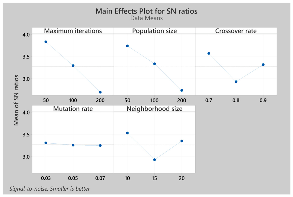
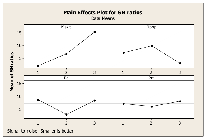
After calculating the value of each experiment and also scaling the values of each experiment, the data were entered into Minitab 16 software for analysis. Since the objective functions are minimization, the highest S/N ratio is the criterion for selecting the parameter values. Figure 3 displays the average S/N ratio plot for the NSGA-II algorithm. As mentioned, the highest S/N ratio is the criterion for selecting the parameter values.

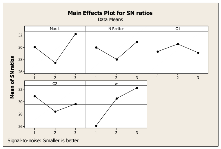
According to the results from Figure 4, the NSGA-II algorithm will have the highest efficiency if the maximum number of iterations is at level 3, the population size is at level 2, the crossover rate is at level 1, and the mutation rate is at level 3. Figure 4 depicts the average S/N ratio plot for the MOPSO algorithm. As mentioned, the highest S/N ratio is the criterion for selecting the parameter values.

According to the results from Figure 4, the MOPSO algorithm will have the highest efficiency if the maximum number of iterations is at level 3, the number of particles is at level 3, the individual learning coefficient is at level 2, the social learning coefficient is at level 1, and the inertia coefficient is at level 3.

Figure 5 illustrates the average S/N ratio plot for the MOEA/D algorithm.

According to the results from Figure 5, the MOEA/D algorithm will have the highest efficiency if the maximum number of iterations is at level 3, the population size is at level 3, the crossover rate is at level 2, the mutation rate is at level 2, and the neighborhood size is at level 2.

5.1. Model Validation

To validate the proposed mathematical model, five varied small-scale instances were solved using the epsilon-constraint method. The total cost objective function was selected as the high-priority objective, while the environmental and social aspects were considered as other priorities. The dimensions of these instances are defined as S1 (3P-3C-5R), S2 (3P-4C-6R), S3 (4P-3C-5R), S4 (4P-5C-5R), and S5 (5P-4C-6R). Due to the model’s non-linearity, the commercial software GAMS 24.1.2 and the BARON solver 14.3.1 solver were utilized for exact solutions. The parameters for all instances were randomly generated based on the uniform distributions shown in

Table 7. Approximate intervals of problem parameters.

Parameter	Approximate Interval
$a_{sj}$	$~u\left(\text{5,10}\right)$
$e_{ij}$	$~u\left(\text{4,8}\right)$
$r_j$	$~u(12,20)$
${\theta }_j$	$~u\left(\text{0,0.5}\right)$
${\lambda }_i^o$	$~u\left(\text{10,25}\right)$
${\lambda }_i^m$	$~u\left(\text{25,40}\right)$
${\lambda }_i^p$	$~u\left(\text{40,50}\right)$
$c_j$	$~u\left(\text{80,100}\right)$
$o_{sj}$	$~u\left(\text{60,80}\right)$
$d_{ij}$	$~u\left(\text{50,70}\right)$
$\beta$	$0.5$
$\gamma$	$0.5$
${\vartheta }_A$	$0.2$
${\vartheta }_B$	$0.2$

.

For each instance, the Pareto optimal solutions were generated. The results for all five instances are consolidated and presented in

Table 8. Set of efficient solutions for the small-sized instances.

Scale	Pareto Front S1: 3P-3C-5R			Pareto Front S2: 3P-4C-6R			Pareto Front S3: 4P-3C-5R			Pareto Front S4: 4P-5C-5R			Pareto Front S5: 5P-4C-6R
#	EA	ET	SA	EA	ET	SA	EA	ET	SA	EA	ET	SA	EA	ET	SA
1	1.814	2.956	0.110	2.297	3.267	0.656	2.332	1.692	0.130	2.607	3.196	1.029	1.611	2.660	0.291
2	1.927	2.366	0.107	2.418	2.914	0.621	2.461	1.541	0.126	2.734	2.881	0.984	1.738	2.384	0.276
3	2.167	2.163	0.105	2.646	2.638	0.583	2.638	1.409	0.122	2.906	2.643	0.946	1.921	2.163	0.263
4	3.124	1.863	0.104	2.913	2.401	0.548	2.927	1.306	0.118	3.168	2.421	0.907	2.218	1.982	0.251
5	3.524	1.529	0.103	3.247	2.182	0.516	3.315	1.218	0.115	3.524	2.186	0.871	2.684	1.811	0.239
6	4.864	1.420	0.102	3.684	1.977	0.487	3.841	1.137	0.112	3.971	1.994	0.834	3.276	1.648	0.228
7	-	-	-	4.196	1.812	0.461	-	-	-	4.463	1.823	0.798	-	-	-
8	-	-	-	-	-	-	-	-	-	5.018	1.674	0.763	-	-	-
9	-	-	-	-	-	-	-	-	-	5.684	1.541	0.731	-	-	-
10	-	-	-	-	-	-	-	-	-	6.437	1.426	0.702	-	-	-
Time (s)	69 (s)			492 (s)			625 (s)			1623 (s)			1328 (s)

Note: EA: economic aspect, ET: environmental aspect, SA: social aspect, ES: efficient solution, P: producers, C: customers, R: retailers.

. These solutions were obtained at an uncertainty rate of 0.5 (moderate scenario).

The results presented in Table 8 clearly demonstrate the inherent trade-offs between the three objective functions across all five test instances. For instance, in case S4, improving the economic objective from a low of 2.607 to a high of 6.437 forces a degradation in the environmental objective from 3.196 to 1.426 and the social objective from 1.029 to 0.702. This inverse relationship, where enhancing economic performance comes at the cost of environmental and social performance, is a consistent pattern observed in every instance. Furthermore, the table highlights the computational complexity of the problem, with the solution time increasing from approximately one minute for S1 to over 27 min for S4, which is expected for this class of NP-hard models. This consistent behavior across varying scales validates the fundamental logic of the proposed model and its capability to generate a rich set of Pareto optimal solutions for decision-makers.

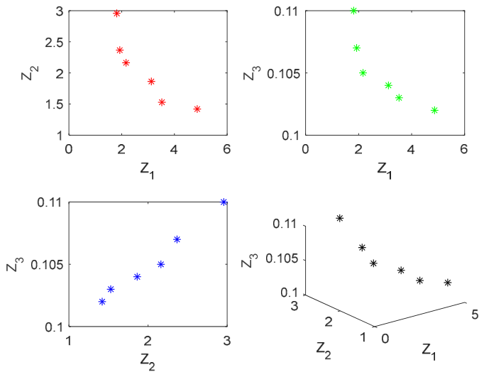
Figure 6 depicts the Pareto front for the small-sized problem (S1: 3-3-5).

As demonstrated in Figure 6, a clear conflict exists between the economic, social, and environmental objectives. In all scenarios, improving one objective, such as reducing CO₂ emissions, necessitates a trade-off in another, such as an increase in total cost. This consistent behavior across varied problem structures validates the fundamental logic of the proposed model.

For the subsequent in-depth sensitivity analysis in Section 5.2, and to maintain clarity and focus, instance S1 is selected as a representative case study. Specifically, the third efficient solution from its Pareto front (economic = 2.167, environmental = 2.163, social = 0.105) is used as the basis for all analyses that follow.

5.2. Sensitivity Analysis

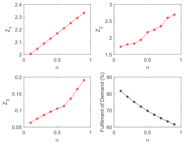
This section performs a sensitivity analysis on the selected baseline: the third efficient solution from instance S1, which corresponds to an economic value of 2.167, an environmental value of 2.163, and a social value of 0.105. Given the uncertainty of the demand parameter and the use of the fuzzy robust programming method to control the mathematical model, a sensitivity analysis is first conducted on the uncertainty rate. In the solved numerical example, the uncertainty rate was assumed to be 0.5, and the percentage of customer demand fulfillment with changes in the values of this parameter is provided in

Table 9. Customer demand fulfillment at different uncertainty rates (%).

Uncertainty Rate	Customer Demand Fulfillment (%)			Average Demand Fulfillment (%)
	Customer 1	Customer 2	Customer 3
0.1	100	100	45.1	81.7%
0.2	100	100	34.7	78.2%
0.3	100	100	25.4	75.1%
0.4	100	100	17	72.3%
0.5	100	100	9.3	69.7%
0.6	100	100	2.3	67.4%
0.7	96.1	100	0	65.3%
0.8	90.3	100	0	63.4%
0.9	100	84.8	0	61.6%

.

The results in Table 9 show that as the uncertainty rate in the supply chain network increases, the average percentage of demand fulfillment decreases. Specifically, in the moderate scenario, this average was 69.7%, and with a 40% increase in demand uncertainty, the average demand fulfillment decreased by 11.62%.

Table 10. Values of objective functions at different uncertainty rates.

Uncertainty Rate	Economic Aspect	Environmental Aspect	Social Aspect
0.1	2.003	1.727	0.063
0.2	2.043	1.796	0.075
0.3	2.086	1.821	0.086
0.4	2.126	1.933	0.096
0.5	2.167	2.163	0.105
0.6	2.208	2.236	0.113
0.7	2.250	2.346	0.135
0.8	2.291	2.594	0.164
0.9	2.231	2.690	0.191

also shows the changes in the values of the objective functions of the problem with variations in the uncertainty rate.

Figure 7 displays the changes in the values of the objective functions with variations in the uncertainty rate.

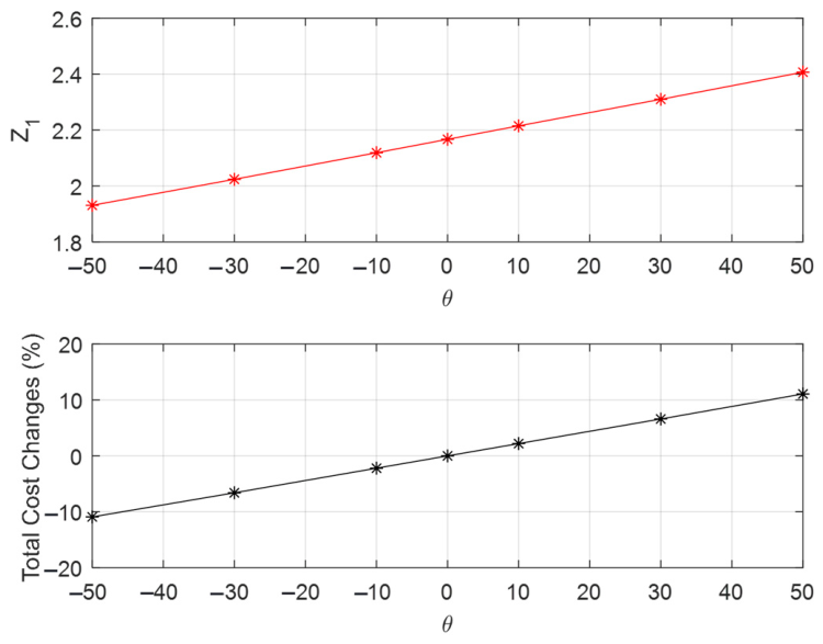
In another analysis, the changes in the economic objective function are examined with respect to variations in the disruption probability of retailers.

Table 11. Value of the total cost objective function with changes in disruption probability.

Probability of Disruption Risk	Total Cost	Changes in Total Cost
50% decrease	1.931	10.91− %
30% decrease	2.024	6.60− %
10% decrease	2.119	2.20− %
No change	2.167	0
10% increase	2.215	2.20+ %
30% increase	2.31	6.60+ %
50% increase	2.407	11.07+ %

shows the value of the total supply chain network cost for 10%, 30%, and 50% changes in the disruption probability of retailers.

Figure 8 indicates the changes in the total supply chain network costs with variations in the disruption probability.

Table 12. Values of objective functions in different retailer warehouse capacity scenarios.

Retailer Warehouse Capacity	Economic Aspect	Environmental Aspect	Social Aspect
50% decrease	2.945	2.648	0.157
30% decrease	2.647	2.347	0.124
10% decrease	2.331	2.268	0.112
No change	2.167	2.163	0.105
10% increase	2.012	2.097	0.094
30% increase	1.948	1.974	0.064
50% increase	1.824	1.856	0.033

analyzes the sensitivity of the problem to changes in the maximum warehouse capacity parameter of the retailer. In this analysis, the retailer’s warehouse capacity is considered 50%, 30%, and 10% lower and higher than its nominal capacity value.

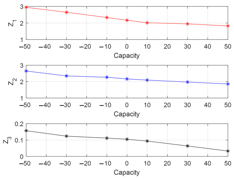
Table 12 illustrates that with an increase in the capacity of retailer warehouses, the need to establish new warehouses decreases. This, in addition to reducing total costs in the supply chain, also reduces carbon dioxide emissions and shortages in the supply chain network. Specifically, a 50% increase in the capacity of retailer warehouses reduced total costs by 15.82%, greenhouse gas emissions by 14.19%, and shortages by 68.57%.

Figure 9 illustrates the changes in the objective functions with variations in retailer warehouse capacity.

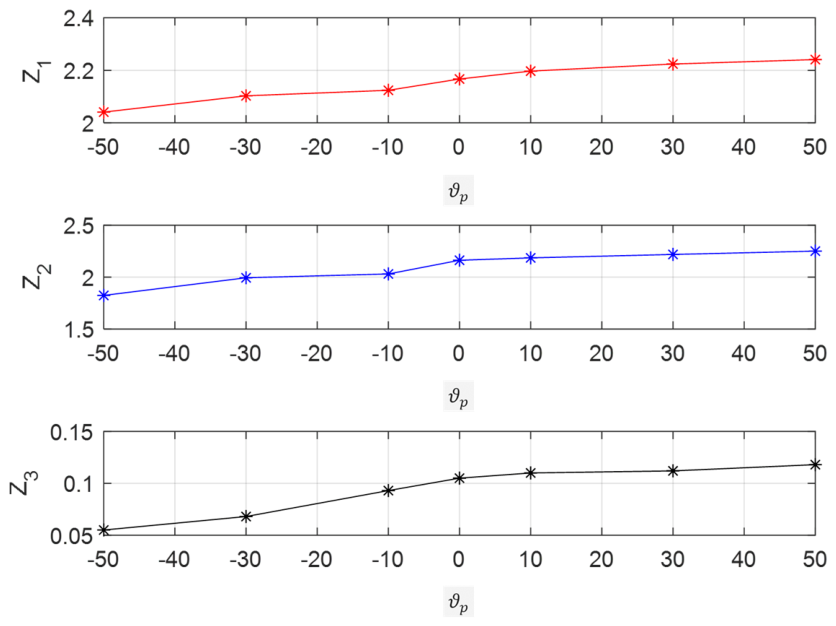
Finally, the impact of the perishability rate on the values of the objective functions is analyzed. In

Table 13. Values of the objective functions in different perishability rate scenarios.

Perishability Rate	Economic Aspect	Environmental Aspect	Social Aspect
50% decrease	2.041	1.824	0.055
30% decrease	2.103	1.994	0.068
10% decrease	2.124	2.031	0.093
No change	2.167	2.163	0.105
10% increase	2.197	2.186	0.110
30% increase	2.224	2.219	0.112
50% increase	2.241	2.251	0.118

, the perishability rate is considered 50%, 30%, and 10% lower and higher than its nominal value.

The results presented in Table 13 indicate that with an increase in the perishability rate, a larger number of products spoil, and to meet demand, the production and distribution amounts have increased. This has led to a relative increase in total costs and greenhouse gas emissions. Although an increase in the perishability rate has also relatively increased the number of shortages, in this analysis, a 50% increase in the perishability rate increased total costs by 3.41%, greenhouse gas emissions by 4.06%, and shortages by 12.38%. This analysis is examined in Figure 10.

5.3. Analysis of Numerical Examples of Different Sizes

5.3.1. Comparison of Efficient Solutions for the Small-Sized Numerical Example

In this section, the efficient solutions obtained from solving the small-sized numerical example using the NSGA-II, MOPSO, and MOEA/D algorithms are examined and compared with the results of the exact epsilon-constraint method. The size of the numerical example is the same as in the previous section (Instance S1), consisting of three production centers, three customers, five potential retailers, and three priority levels for retailers. The input parameters of the problem are also considered identical to those in the previous section. Accordingly,

Table 14. Set of efficient solutions obtained from solving the small-sized numerical example using different methods.

ES	Epsilon-Constraint			NSGA-II			MOPSO			MOEA/D
	EA	ET	SA	EA	ET	SA	EA	ET	SA	EA	ET	SA
1	1.814	2.956	0.110	1.814	2.956	0.110	1.814	2.956	0.110	1.837	3.742	0.024
2	1.927	2.366	0.107	1.854	2.732	0.108	1.823	2.823	0.109	1.725	5.014	0.045
3	2.167	2.163	0.105	1.927	2.366	0.107	1.877	2.524	0.108	1.698	2.385	0.067
4	3.124	1.863	0.104	2.254	2.114	0.105	1.927	2.366	0.107	1.578	3.271	0.045
5	3.524	1.529	0.103	2.915	1.793	0.104	2.124	2.124	0.106	1.662	2.385	0.120
6	4.864	1.420	0.102	3.524	1.529	0.103	2.348	1.934	0.105	1.507	4.963	0.093
7	-	-	-	3.812	1.517	0.103	2.974	1.744	0.104	1.523	3.422	0.120
8	-	-	-	3.934	1.495	0.103	3.524	1.529	0.103	1.645	2.741	0.327
9	-	-	-	4.265	1.466	0.102	4.745	1.315	0.102	1.621	2.385	0.569
10	-	-	-	4.864	1.420	0.102	-	-	-	1.516	3.814	0.120

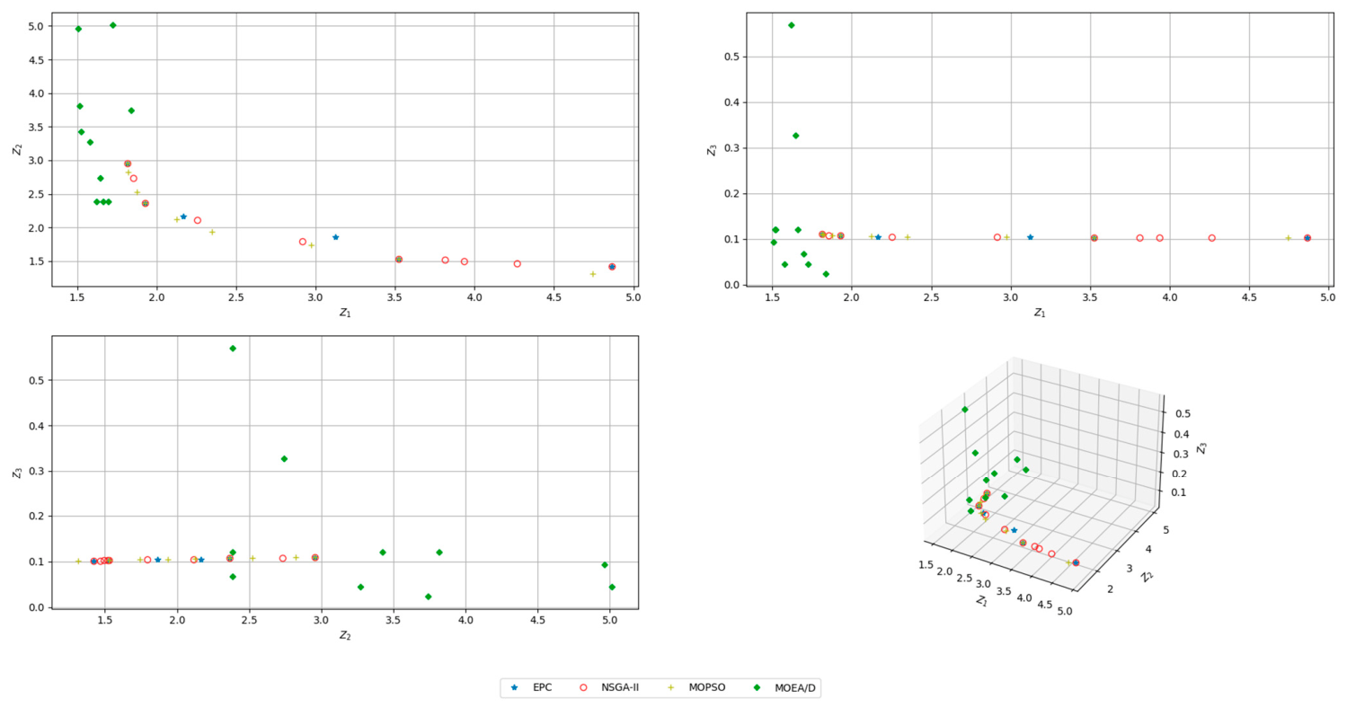
Note: EA: economic aspect, ET: environmental aspect, SA: social aspect, ES: efficient solution.

presents the set of efficient solutions obtained from solving this small-sized numerical example using the epsilon-constraint method, NSGA-II, MOPSO, and MOEA/D.

Table 14 also demonstrates that the metaheuristic algorithms (NSGA-II, MOPSO, and MOEA/D), similar to the epsilon-constraint method, have reached logical results. Specifically, as the amount of carbon dioxide in the supply chain network decreases, the total costs have increased. On the other hand, with a decrease in shortages in the supply chain network, due to the increased amount of demand and transportation, the total costs have again increased. It is worth noting that for the MOEA/D algorithm, the solutions reflect genuine non-dominated trade-offs in a three-dimensional space. In such a multi-objective environment, optimizing one objective does not necessarily result in a monotonic trend across all other objectives simultaneously, which explains the fluctuations observed in the environmental and social values for certain solution points. Figure 11 compares the Pareto front obtained from solving the small-sized numerical example using different solution methods.

Since the number of efficient solutions obtained from the solution methods is different, the comparison indices proposed in the parameter tuning section are used to compare the results of the exact method and the three metaheuristic algorithms. Accordingly,

Table 15. Comparison of efficient solution indices between two solution methods.

Index	Epsilon-Constraint	NSGA-II	MOPSO	MOEA/D
NPF	6	10	9	11
MSI	4.22	4.37	4.18	2.775
SM	0.48	0.36	0.38	0.215
CPT	10.33	5.18	4.16	0.517

indicates the efficient solution indices among the four different solution methods in the small-sized numerical example.

The results in Table 15 show that the MOEA/D algorithm performed significantly better in the CPT, SM, and NPF indices. Specifically, 11 efficient solutions were obtained by MOEA/D, 10 by NSGA-II, 9 by MOPSO, and 6 by the epsilon-constraint method. Meanwhile, the NSGA-II algorithm demonstrated better performance in the MSI index compared to the other methods. Furthermore, the CPU times (CPT) of all three metaheuristic algorithms are considerably lower than the solution time of the exact method, with MOEA/D being the fastest.

5.3.2. Examining Multiple Numerical Examples of Large Sizes

After analyzing the small-sized numerical example and comparing it with the exact method, this section evaluates the performance of the three metaheuristic algorithms (NSGA-II, MOPSO, and MOEA/D) across 15 large-scale instances. The dimensions of these instances are detailed in

Table 16. Instance size.

Instants	S	J	I	G
1	4	5	4	3
2	4	5	5	3
3	5	6	6	4
4	5	6	7	4
5	6	8	8	5
6	6	8	9	5
7	7	10	10	6
8	7	10	11	6
9	8	12	12	8
10	8	12	14	8
11	9	15	16	12
12	9	15	18	12
13	10	18	20	14
14	12	18	24	16
15	15	20	25	16

.

To account for the stochastic nature of the metaheuristic algorithms, NSGA-II, MOPSO, and MOEA/D were executed for 10 independent replications using different random seeds for each problem instance. The results in

Table 17. Findings from solving different instances.

Instant	NSGA-II				MOPSO				MOEA/D
	CPT	SM	MSI	NPF	CPT	SM	MSI	NPF	CPT	SM	MSI	NPF
1	9.11	0.555	2.85	43	8.75	0.529	3.06	45	2.749	0.211	6.089	13
2	9.28	0.647	6.33	39	8.99	0.543	7.98	38	2.532	0.656	5.83	12
3	9.34	0.517	6.5	43	9	0.432	7.36	48	2.599	0.37	7.167	16
4	9.35	0.575	7.94	44	8.98	0.532	8.38	42	2.586	0.675	11.104	16
5	9.42	0.486	13.49	46	8.95	0.398	14.33	39	2.795	0.775	12.703	12
6	9.64	0.435	15.72	40	9.23	0.355	16.61	37	2.726	0.908	9.819	14
7	10.5	0.398	17.79	40	9.98	0.364	18.28	43	3.34	0.353	12.765	11
8	10.61	0.367	20.29	38	10.09	0.47	20.48	35	3.067	0.275	13.388	11
9	10.97	0.431	29.81	36	10.45	0.561	30.84	39	3.825	0.618	20.164	13
10	11.27	0.621	30.56	43	10.85	0.402	30.62	42	4.068	0.43	23.612	15
11	11.95	0.556	36.86	50	11.59	0.546	37.51	41	5.835	0.986	422.432	19
12	12.38	0.538	42.39	50	11.91	0.375	43.16	49	6.594	0.992	425.753	15
13	14.33	0.442	52.67	50	13.86	0.597	53.49	41	8.544	0.823	364.249	14
14	18.02	0.604	76.24	50	17.37	0.533	75.88	50	11.162	0.818	321.267	13
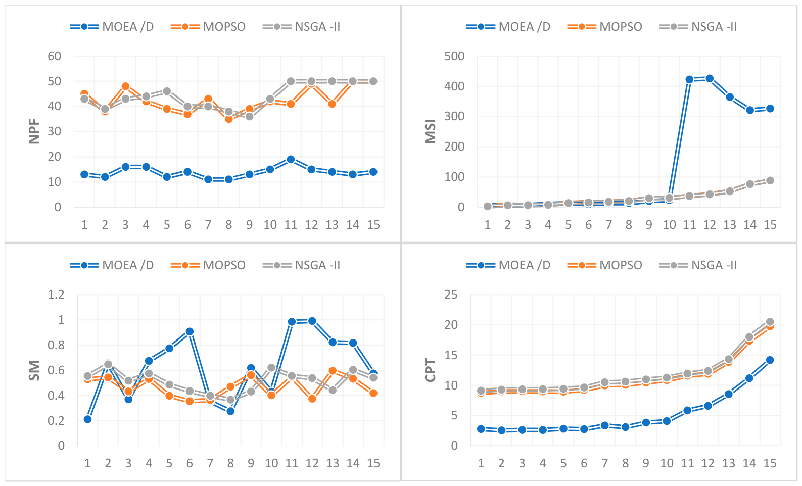
15	20.54	0.541	88.05	50	19.76	0.419	88.22	50	14.185	0.575	326.632	14

present the average values of the comparison indices obtained from these independent runs to illustrate the performance of the algorithms. The results indicate that as the instance size increases, the values of MSI and CPT also increase. The exponential increase in the CPT value, proportional to the problem size and the non-linearity of the problem, empirically suggests the high computational complexity of the proposed model and justifies the application of metaheuristic algorithms. Figure 12 shows the obtained indices for each instance using the NSGA-II, MOPSO, and MOEA/D algorithms.

Table 18. Examining the significant differences in indices at a 95% confidence level using ANOVA.

Index	F-Value	p-Value	Result at 95% Confidence Level	Winner (Best Performance)
NPF	296.84	0.000	Significant difference	MOPSO/NSGA-II
MSI	4.34	0.019	Significant difference	NSGA-II
SM	1.63	0.208	No significant difference	-
CPT	18.84	0.000	Significant difference	MOEA/D

examines the significant differences in the comparison indices at a 95% confidence level among the three solution methods used in this research. Since three algorithms are being compared, a one-way Analysis of Variance (ANOVA) was conducted based on the results across the multiple instances.

Based on the ANOVA results in Table 18, there is a statistically significant difference among the algorithms in the NPF, MSI, and CPT indices ($p\text{-}\mathrm{value}<0.05$). To identify the specific pairwise differences causing these omnibus significant results, a Tukey HSD post-hoc test was conducted. For the NPF index, the post-hoc analysis revealed that while both MOPSO and NSGA-II generate a significantly higher number of Pareto solutions compared to MOEA/D, there is no statistically significant difference between MOPSO and NSGA-II themselves, statistically justifying their shared position as the best-performing algorithms in this category. Furthermore, MOEA/D demonstrates a clear superiority in computational time (CPT), solving the models significantly faster than the other two methods. However, NSGA-II and MOPSO provide solutions with a more balanced dispersion and lower deviation (better MSI), whereas MOEA/D struggles severely with MSI in larger instances. Considering the spacing metric (SM), the ANOVA confirms no statistically significant difference among the three algorithms ($p\text{-}\mathrm{value}=0.208$). Ultimately, given the robust performance of MOPSO in providing a high number of Pareto solutions, competitive spacing, and acceptable solving times, it is selected as a highly efficient and reliable algorithm for solving the proposed large-scale model.

5.4. Practical Implications

The findings of this study offer actionable and quantifiable insights for supply chain managers, policymakers, and sustainability practitioners aiming to enhance network resilience amid disruptions and demand uncertainty. Rather than relying on generic strategies, managers can utilize the empirical trade-offs identified in our sensitivity analyses to prioritize their investments.

First, strategic retailer selection and proactive risk mitigation are paramount. Our analysis demonstrates that a $50\%$ increase in the disruption probability of retailers leads to an $11.07\%$ surge in total supply chain costs. Consequently, managers should not select retailers based solely on proximity or nominal costs, but must factor in reliability. Investing in contingency plans, such as backup suppliers or resilient infrastructure, is highly justified to prevent these significant financial losses, especially in industries where unmet demand directly damages brand reputation.

Furthermore, dynamic demand and uncertainty management dictate the efficiency of the supply chain. The integration of fuzzy robust programming in our model revealed that a $40\%$ escalation in demand uncertainty causes the average demand fulfillment rate to drop by $11.62\%$. To combat this, firms must invest in real-time demand forecasting tools and agile inventory policies. The sensitivity results particularly highlight the critical role of warehouse capacity: a $50\%$ strategic expansion in retailer warehouse capacity not only decreases total costs by $15.82\%$ by minimizing the need for redundant facilities, but also drastically reduces product shortages by $68.57\%$ and greenhouse gas emissions by $14.19\%$. Therefore, targeted investments in localized storage capacity yield simultaneous economic, social, and environmental dividends.

Addressing product perishability is another major managerial imperative. The model shows that a $50\%$ increase in the perishability rate inflates total costs by $3.41\%$ and greenhouse gas emissions by $4.06\%$, while increasing product shortages by $12.38\%$. Supply chain managers handling perishable goods must prioritize IoT-enabled cold chain technologies and swift routing to monitor and suppress spoilage rates, thereby protecting profit margins and sustainability targets.

Finally, at the operational and algorithmic level, decision-makers are encouraged to integrate advanced metaheuristics into their decision-support systems for large-scale planning. While our results show that MOEA/D offers the fastest computational time (CPT), MOPSO provides a highly balanced performance, yielding a robust number of Pareto solutions without sacrificing stability. By adopting these quantified strategies and computational tools, organizations can build supply chains that are not only economically viable but also environmentally responsible and socially equitable, directly aligning with global sustainability agendas.

5.5. Theoretical Implications

The findings of this study contribute significantly to the theoretical discourse on sustainable supply chain network design by integrating disruption risks and demand uncertainty into a multi-objective optimization framework. The proposed model aligns with and extends prior research, such as [22], which emphasized robust stochastic optimization for disruption-prone networks, and ref. [3], which explored incentive mechanisms under demand uncertainty. However, this study advances the literature by incorporating fuzzy robust programming to handle demand ambiguity and probabilistic disruptions simultaneously, a combination less explored in existing works. The results corroborate the trade-offs between economic, environmental, and social objectives, as highlighted by [1], but further quantify these trade-offs through detailed sensitivity analyses, providing deeper mathematical insights into the interdependencies among cost, emissions, and shortages. Furthermore, the evaluation of advanced metaheuristics (NSGA-II, MOPSO, and MOEA/D) provides empirical validation for algorithm selection in complex supply chain problems. While MOEA/D accelerates the solution process, the robust performance of MOPSO in large-scale scenarios resonates with [13], which advocated for balanced metaheuristics in NP-hard optimization. By bridging gaps between sustainability theory and practical modeling techniques, this research reinforces the need for holistic approaches in supply chain design and identifies underexplored areas, such as hybrid algorithmic frameworks, for future theoretical exploration.

6. Conclusions

This research focused on modeling a multi-objective sustainable supply chain network under disruption and demand uncertainty. The considered model included three levels: production centers, retailers, and customers, with the aim of selecting sustainable retailers from potential candidates and allocating production centers and customers to them. To achieve these strategic and tactical decisions, three objective functions were considered: minimizing total costs, minimizing carbon dioxide emissions, and minimizing product shortages. The designed model, due to the use of disruption-related equations, is structurally non-linear, and fuzzy robust programming was employed to handle demand ambiguity.

To validate the mathematical model, five small-scale problem instances were solved using the exact epsilon-constraint method. Analysis of the Pareto fronts and efficient solutions confirmed the direct conflicts among the objectives: as shortages decrease, the total costs of the supply chain network increase. Similarly, decreasing carbon dioxide emissions also increases total costs. Conversely, the trends of the second and third objective functions are aligned; specifically, a decrease in emissions generally corresponds to a decrease in shortages.

By examining the problem outputs and conducting sensitivity analyses, it was observed that as the uncertainty rate increases, demand shifts towards the pessimistic (higher demand) scenario, leading to increased total costs, emissions, and shortages. Furthermore, an increase in the disruption probability of retailers significantly increased total costs. Specifically, a $50\%$ increase in the disruption probability of retailers led to an $11.07\%$ increase in total costs. Conversely, expanding retailer warehouse capacity reduced the need to establish new facilities. A $50\%$ increase in capacity reduced total costs by $15.82\%$, greenhouse gas emissions by $14.19\%$, and shortages by $68.57\%$. Finally, a $50\%$ increase in the perishability rate led to more spoiled products, which increased total costs by $3.41\%$, emissions by $4.06\%$, and shortages by $12.38\%$.

To solve the model in larger sizes, three advanced multi-objective algorithms—NSGA-II, MOPSO, and MOEA/D—were implemented. The comparison between the algorithms was conducted using four indices: NPF, MSI, SM, and CPT, supported by ANOVA statistical testing over multiple independent runs. The results demonstrated that while the MOEA/D algorithm significantly outperformed the others in terms of computational time (CPT), the MOPSO and NSGA-II algorithms demonstrated higher efficiency in solution quality metrics (NPF and MSI). Based on the ANOVA results, MOPSO is selected as the most efficient and balanced algorithm for this problem structure. The analysis of larger-sized numerical examples further confirmed the high computational difficulty of the proposed model, and the solution time increases exponentially with the problem size.

Limitations and Future Research Directions

This study has some limitations that should be acknowledged. Notably, the implementation of a greedy priority-based allocation rule within the metaheuristic algorithms, while computationally efficient, may constrain the solution search space and introduce a potential bias toward local optima, limiting the exploration of more complex global trade-offs. To address this, future research directions could explore non-greedy or adaptive decoding strategies. Furthermore, future studies could expand the supply chain into a closed-loop system while integrating broader sustainability metrics, as well as examining routing strategies between retailers and customers to enhance operational efficiency. Additionally, investigating potential disruptions at production centers and their impact on supply chain resilience would be valuable, along with the application of hybrid algorithms to improve problem-solving approaches in this context.

References

- Govindan, K.; Jafarian, A.; Nourbakhsh, V. Nourbakhsh, Designing a sustainable supply chain network integrated with vehicle routing: A comparison of hybrid swarm intelligence metaheuristics. Comput. Oper. Res. 2019, 110, 220–235. [Google Scholar] [CrossRef] [Scilit]
- Rahmativala, S.; Ghahremani, J. A robust optimization method for hybrid flow shop scheduling with uncertain setup times. Decis. Anal. J. 2025, 16, 100609. [Google Scholar] [CrossRef] [Scilit]
- Wang, W.; Zhang, Y.; Zhang, W.; Gao, G.; Zhang, H. Incentive mechanisms in a green supply chain under demand uncertainty. J. Clean. Prod. 2021, 279, 123636. [Google Scholar] [CrossRef] [Scilit]
- Ilgin, M.A.; Gupta, S.M. Environmentally conscious manufacturing and product recovery (ECMPRO): A review of the state of the art. J. Environ. Manag. 2010, 91, 563–591. [Google Scholar] [CrossRef] [Scilit] [PubMed]
- Ahi, P.; Searcy, C. Measuring social issues in sustainable supply chains. Meas. Bus. Excel. 2015, 19, 33–45. [Google Scholar] [CrossRef] [Scilit]
- Klassen, R.D.; Vereecke, A. Social issues in supply chains: Capabilities link responsibility, risk (opportunity), and performance. Int. J. Prod. Econ. 2012, 140, 103–115. [Google Scholar] [CrossRef] [Scilit]
- Hutchins, M.J.; Sutherland, J.W. An exploration of measures of social sustainability and their application to supply chain decisions. J. Clean. Prod. 2008, 16, 1688–1698. [Google Scholar] [CrossRef] [Scilit]
- Balcik, B.; Beamon, B.M. Facility location in humanitarian relief. Int. J. Logist. Res. Appl. 2008, 11, 101–121. [Google Scholar] [CrossRef] [Scilit]
- Özdamar, L.; Ertem, M.A. Models, solutions and enabling technologies in humanitarian logistics. Eur. J. Oper. Res. 2015, 244, 55–65. [Google Scholar] [CrossRef] [Scilit]
- Aldrighetti, R.; Battini, D.; Ivanov, D.; Zennaro, I. Costs of resilience and disruptions in supply chain network design models: A review and future research directions. Int. J. Prod. Econ. 2021, 235, 108103. [Google Scholar] [CrossRef] [Scilit]
- Wang, X.; Chen, G.; Xu, S. Bi-objective green supply chain network design under disruption risk through an extended NSGA-II algorithm. Clean. Logist. Supply Chain 2022, 3, 100025. [Google Scholar] [CrossRef] [Scilit]
- Atmayudha, A.; Syauqi, A.; Purwanto, W.W. Green logistics of crude oil transportation: A multi-objective optimization approach. Clean. Logist. Supply Chain 2021, 1, 100002. [Google Scholar] [CrossRef] [Scilit]
- Abdel-Basset, M.; Mohamed, R.; Sallam, K.; Elhoseny, M. A novel decision-making model for sustainable supply chain finance under uncertainty environment. J. Clean. Prod. 2020, 269, 122324. [Google Scholar] [CrossRef] [Scilit]
- Sahebjamnia, N.; Fathollahi-Fard, A.M.; Hajiaghaei-Keshteli, M. Sustainable tire closed-loop supply chain network design: Hybrid metaheuristic algorithms for large-scale networks. J. Clean. Prod. 2018, 196, 273–296. [Google Scholar] [CrossRef] [Scilit]
- Montoya-Torres, J.R. Designing sustainable supply chains based on the Triple Bottom Line approach. In Proceedings of the 2015 4th International Conference on Advanced Logistics and Transport (ICALT), Valenciennes, France, 20–22 May 2015. [Google Scholar]
- Pellegrino, R.; Gaudenzi, B.; Fraccascia, L.; Genovese, A.; Basile, L.J. Can the Adoption of Circular Economy Practices Foster Supply Chain Resilience and Performance Improvements? Bus. Strat. Environ. 2026, 35, 438–457. [Google Scholar] [CrossRef] [Scilit]
- Echefaj, K.; Charkaoui, A.; Cherrafi, A.; Ivanov, D. Design of resilient and viable sourcing strategies in intertwined circular supply networks. Ann. Oper. Res. 2024, 337, 459–498. [Google Scholar] [CrossRef] [Scilit]
- Sutar, P.S.; Kolte, G.C.; Yamini, S. Food supply chain disruptions and its resilience: A framework and review for resilience strategies in the digital era. Opsearch 2026, 63, 164–198. [Google Scholar] [CrossRef] [Scilit]
- Ishaq, S.; Tanveer, U.; Hoang, T.G.; Samuel, F.W. From Linear to Circular: Capabilities, Defensive Reasoning and Supply Chain Collaborations in Manufacturers’ Circular Economy Transition. Br. J. Manag. 2026, 37, e12932. [Google Scholar] [CrossRef] [Scilit]
- Massari, G.F.; Nacchiero, R.; Giannoccaro, I. The resilience of planned and self-organised circular economy networks: A novel simulation approach. Int. J. Prod. Res. 2026, 64, 4236–4270. [Google Scholar] [CrossRef] [Scilit]
- Yahyapour Ganji, V.; Hozan, E.; Babolhavaeji, P.; Tajally, A.; Ghanavati-Nejad, M. A robust design of a circular supply chain network based on the resilience and responsiveness dimensions: A data-driven model. Socio-Econ. Plan. Sci. 2025, 101, 102294. [Google Scholar] [CrossRef] [Scilit]
- Jabbarzadeh, A.; Haughton, M.; Khosrojerdi, A. Closed-loop supply chain network design under disruption risks: A robust approach with real world application. Comput. Ind. Eng. 2018, 116, 178–191. [Google Scholar] [CrossRef] [Scilit]
- Yan, S.; Ji, X. Supply chain network design under the risk of uncertain disruptions. Int. J. Prod. Res. 2020, 58, 1724–1740. [Google Scholar] [CrossRef] [Scilit]
- Ali, S.M.; Rahman, H.; Tumpa, T.J.; Rifat, A.A.M.; Paul, S.K. Examining price and service competition among retailers in a supply chain under potential demand disruption. J. Retail. Consum. Serv. 2018, 40, 40–47. [Google Scholar] [CrossRef] [Scilit]
- Zarei, N.; Azari, A.; Heidari, M.M. Improvement of the performance of NSGA-II and MOPSO algorithms in multi-objective optimization of urban water distribution networks based on modification of decision space. Appl. Water Sci. 2022, 12, 133. [Google Scholar] [CrossRef] [Scilit]
- Goodarzian, F.; Shishebori, D.; Nasseri, H.; Dadvar, F. A bi-objective production-distribution problem in a supply chain network under grey flexible conditions. RAIRO-Oper. Res. 2021, 55, 1971–2000. [Google Scholar] [CrossRef] [Scilit]
- Akbari-Aghghaleh, Z.; Mozdgir, A.; Seyedi, I.; Messina, E. Designing a perishable closed-loop poultry supply chain: Metaheuristic approaches and model evaluation. Environ. Dev. Sustain. 2025, in press. [Google Scholar] [CrossRef] [Scilit]
- Rezasoltani, A.; Mohaghar, A.; Khatami Firouzabadi, S.M.A.; Khani, A.M. Designing Sustainable Supply Chains for Perishable Products Under Uncertainty: A Fuzzy Robust Multi-Objective Possibilistic Approach. Iran. J. Fuzzy Syst. 2026, 23, 119–139. [Google Scholar]
- Kim, J.; Qiu, R.; Jon, J.; Sun, M. Multi-objective programming for multi-period multi-product closed-loop supply chain network design: A fuzzy robust optimization approach. Environ. Dev. Sustain. 2025, 27, 10203–10239. [Google Scholar] [CrossRef] [Scilit]
- Taqi, H.M.M.; Ali, S.M.; Fathollahi-Fard, A.M.; Paul, S.K.; Kabir, G. Supply chain network design with flexibility, resiliency, and sustainability. Sustain. Resilient Infrastruct. 2025, 11, 389–419. [Google Scholar] [CrossRef] [Scilit]
- Nozari, H.; Tavakkoli-Moghaddam, R.; Gharemani-Nahr, J. A Neutrosophic Fuzzy Programming Method to Solve a Multi-depot Vehicle Routing Model under Uncertainty during the COVID-19 Pandemic. Int. J. Eng. 2022, 35, 360–371. [Google Scholar] [CrossRef] [Scilit]
- Jiménez, M.; Arenas, M.; Bilbao, A.; Rodríguez, M.V. Linear programming with fuzzy parameters: An interactive method resolution. Eur. J. Oper. Res. 2007, 177, 1599–1609. [Google Scholar] [CrossRef] [Scilit]
- Pishvaee, M.; Torabi, S. A possibilistic programming approach for closed-loop supply chain network design under uncertainty. Fuzzy Sets Syst. 2010, 161, 2668–2683. [Google Scholar] [CrossRef] [Scilit]
- Deb, K.; Pratap, A.; Agarwal, S.; Meyarivan, T. A fast and elitist multiobjective genetic algorithm: NSGA-II. IEEE Trans. Evol. Comput. 2002, 6, 182–197. [Google Scholar] [CrossRef] [Scilit]
- Zhang, Q.; Li, H. MOEA/D: A Multiobjective Evolutionary Algorithm Based on Decomposition. IEEE Trans. Evol. Comput. 2007, 11, 712–731. [Google Scholar] [CrossRef] [Scilit]
- Mavrotas, G. Effective implementation of the ε-constraint method in Multi-Objective Mathematical Programming problems. Appl. Math. Comput. 2009, 213, 455–465. [Google Scholar]
Figure 1.
Illustration of the two-point crossover mechanism in the NSGA-II algorithm (colored arrows represent the movement of genes, and letters denote specific values).
Figure 2.
Illustration of the mutation crossover mechanism in the NSGA-II algorithm.
Figure 3.
Average S/N ratio plot in the NSGA-II algorithm.
Figure 4.
Average S/N ratio plot in the MOPSO algorithm.
Figure 5.
Average S/N ratio plot in the MOEA/D algorithm.
Figure 6.
The Pareto front resulting from solving the small-sized problem (asterisks indicate the Pareto-optimal solutions).
Figure 7.
Changes in the values of the objective functions with variations in the uncertainty rate.
Figure 8.
Changes in total supply chain network costs with variations in disruption probability.
Figure 9.
Changes in the objective functions with variations in retailer warehouse capacity.
Figure 10.
Changes in the values of objective functions at different perishability rates.
Figure 11.
Comparing the Pareto front in numerical example.
Figure 12.
Indices obtained from solving various problem instances with different sizes.