Revenue–Expenditure Consistency and the Sustainability of Public Finances in the Euro-Area Periphery: Evidence from Five Southern European Economies, 1999–2023

Abstract

How the two sides of the government budget are causally linked bears directly on the design of fiscal consolidation. This paper examines the relationship between government revenue and expenditure in five Southern European economies over 1999–2023, applying three causality procedures, cointegration analysis and structural-break tests to identical quarterly data. The central finding is that the causal classifications are not robust: three of the five economies are classified differently depending on the procedure used, Portugal differently under each, and expressing both aggregates as shares of GDP alters the results again. Conclusions drawn from any single test are therefore unreliable. What does survive changes in specification is the direction of adjustment: revenue closes budgetary imbalances in Italy, and expenditure closes them in Spain, Portugal and Cyprus. Analysis of expenditure by function shows that consolidation did not reduce the size of these budgets but recomposed them, with public investment falling by between nine and forty per cent and not recovering. Fiscal rules should accordingly match the instrument to the adjusting side and protect capital expenditure explicitly.

1. Introduction

Sustainable development rests on the fiscal capacity of the state to finance it. Public investment in education, health, social protection, climate adaptation and the energy transition is delivered through the government budget, and a government that cannot satisfy its intertemporal budget constraint cannot sustain that expenditure. Fiscal sustainability is therefore not merely an accounting condition but a precondition for the Sustainable Development Goals, and it is recognised as such in SDG 17.1, which calls for strengthening domestic resource mobilisation and improving domestic capacity for tax and other revenue collection. The euro-area periphery is a demanding setting in which to examine that precondition. Between 1999 and 2023, Greece, Spain, Italy, Portugal and Cyprus experienced the introduction of the euro, a global financial crisis, a sovereign-debt crisis with associated adjustment programmes, a pandemic, and the energy-price shock that followed it. Each episode tested the capacity of the state to align revenue with expenditure while protecting the spending on which long-run development depends. This paper asks two connected questions for these five economies: whether public finances satisfied the intertemporal budget constraint over the period, and which side of the budget adjusts to the other. Taxation also shapes the microeconomic base of that capacity: evidence from EU economies links tax burdens to the performance of the small- and medium-sized enterprises on which the revenue base rests [1].

The relationship between government revenue and government expenditure is one of the most enduring questions in public economics. How the two sides of the budget are causally linked has direct implications for the design of fiscal consolidation: if revenues drive spending, raising taxes may be an effective route to deficit reduction; if spending drives revenues, expenditure restraint is the more promising lever; and if the two are jointly determined or causally independent, the sequencing of consolidation measures matters less than their overall magnitude. The question has acquired renewed urgency in the euro-area periphery, where successive sovereign-debt and pandemic shocks have forced repeated reassessments of the appropriate fiscal stance.

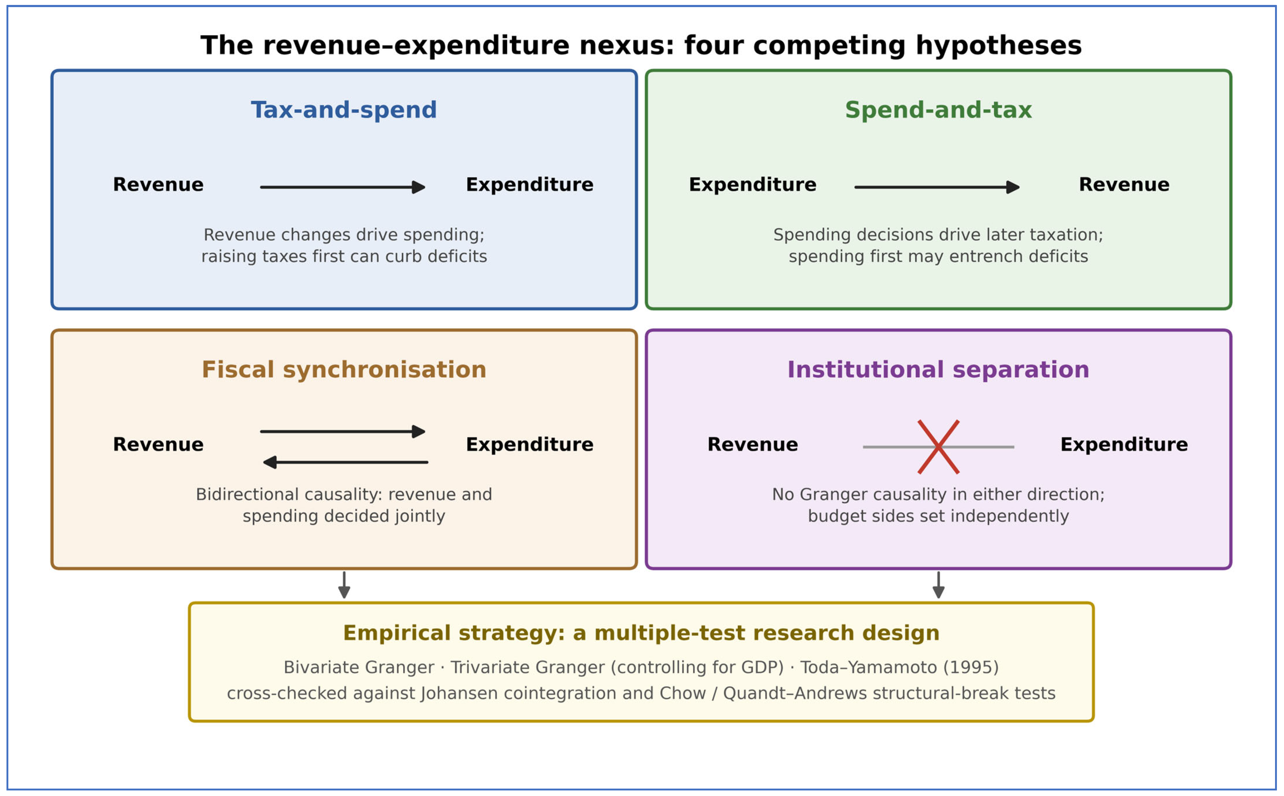
Four hypotheses structure the empirical literature on the revenue–expenditure nexus. The tax-and-spend hypothesis, associated with Friedman [2] and Buchanan and Wagner [3], holds that changes in revenue precede and cause changes in expenditure, though the two authors disagree on the sign of the relationship. The spend-and-tax hypothesis, advanced by Peacock and Wiseman [4] and consistent with Barro’s [5] tax-smoothing framework, reverses the direction: governments determine spending first and adjust taxation to finance it. The fiscal-synchronisation hypothesis, rooted in Musgrave [6] and Meltzer and Richard [7], posits that revenue and expenditure decisions are taken jointly, generating bidirectional causality. Finally, the institutional-separation (or fiscal-independence) hypothesis of Baghestani and McNown [8] holds that the two budget components are determined by separate institutional processes, so that neither Granger-causes the other.

This paper tests these four hypotheses for five Southern European economies—Greece, Spain, Italy, Portugal and Cyprus—using quarterly data spanning 1999Q1 to 2023Q4. These economies share a common monetary framework, comparable exposure to the 2010–2012 sovereign-debt crisis, and broadly similar fiscal-governance constraints under the European fiscal framework, which makes them a coherent group for comparative analysis while still exhibiting meaningful institutional heterogeneity. Their fiscal trajectories over the sample period encompass the introduction of the euro, the global financial crisis, the euro-area debt crisis and associated adjustment programmes, the COVID-19 shock, and the energy-price crisis of 2021–2023—a sequence of events that provides substantial variation against which to identify revenue–expenditure dynamics. The last of these episodes bore directly on the budget balance: between September 2021 and March 2023 European Union member states allocated some EUR 646 billion to measures shielding households and firms from higher energy prices, and the Southern European economies were among the larger spenders relative to GDP [9]. Because these measures were concentrated in the final years of the sample, they fall within the post-2020 sub-period examined in Section 3.7.

This paper makes three connected contributions. First, it establishes whether the intertemporal budget constraint held in each of the five economies and, through the cointegrating slope, how far each budget stood from full long-run coverage of expenditure by revenue. Second, it identifies which side of the budget has historically borne the adjustment, which bears directly on the design of consolidation. Third, it establishes how far the causal classification of each country depends on the testing procedure, and therefore how much confidence the existing literature’s conclusions can support. Rather than relying on a single causality test—the common practice in much of the older literature—we adopt a multiple-test research design and ask whether the fiscal classification a researcher would assign to each country is robust to the choice of method. We combine three complementary causality approaches (bivariate Granger, trivariate Granger conditioning on output, and the Toda–Yamamoto procedure that is valid regardless of the integration and cointegration properties of the data) and cross-check them against Johansen cointegration analysis and two families of structural-break tests. The central empirical finding is that classifications are not robust: the inference one draws depends materially on the method used, on whether output is included as a conditioning variable, and on whether structural breaks are accommodated. This sensitivity is itself the result of interest, and it cautions against the single-test inference that remains common in applied fiscal-policy work.

The remainder of the paper is organised as follows. Section 2 reviews the related empirical literature, describes the data and the econometric methodology. Section 3 reports the results, beginning with the time-series properties of the data and proceeding through the cointegration, causality and structural-break analyses. Section 4 discusses the findings and their robustness, and Section 5 concludes with policy implications and limitations.

1.1. Fiscal Sustainability and the Intertemporal Budget Constraint

The revenue–expenditure nexus is directly connected to the sustainability of public finances. If government revenue and expenditure are cointegrated, the two series share a long-run equilibrium relationship, the discounted value of future debt converges to zero, and the government satisfies its intertemporal budget constraint. This is the basis of the cointegration test of fiscal sustainability introduced by Hamilton and Flavin [10] and developed by Trehan and Walsh [11], Hakkio and Rush [12], and Quintos [13]. Hakkio and Rush [12] show that cointegration with a slope coefficient of unity implies strong sustainability, whereas cointegration with a slope between zero and one implies weak sustainability: the government meets its constraint, but debt grows faster than the capacity to service it, and the arrangement may not survive market scrutiny. Quintos [13] extends the framework to accommodate structural shifts in the deficit process, which is directly relevant to economies that underwent adjustment programmes. The absence of cointegration implies that the constraint is violated and that the fiscal position is not sustainable over the sample considered. Evidence for the European Union is mixed. Neaime [14] reports unsustainable deficits and debts in several member states, and Legrenzi and Milas [15] find that Italy meets its intertemporal budget constraint within a nonlinear error-correction framework, with the burden of adjustment falling on the tax side. For Southern Europe, Trachanas and Katrakilidis [16] find fiscal deficits to be weakly sustainable in Italy, Greece and Spain over 1970–2010, with asymmetric budgetary adjustment in Italy and Spain. Ramos-Herrera and Prats [17] reach similarly mixed verdicts for twenty EU economies using panel ARDL and threshold methods, underlining that sustainability conclusions depend on the econometric framework employed.

Two qualifications frame what this test can establish. First, cointegration between revenue and expenditure is a necessary but not a sufficient condition for solvency. It confirms that the two aggregates do not drift apart without limit, but it does not by itself establish that the debt ratio is on a convergent path. Second, in high-debt euro-area economies the trajectory of the debt-to-GDP ratio depends on the primary balance, nominal output growth, inflation, the effective interest rate on outstanding debt and the resulting interest–growth differential, none of which enters a bivariate revenue–expenditure system. Where the differential is unfavourable, a budget that satisfies the revenue–expenditure condition may still generate a rising debt ratio. The analysis that follows should therefore be read as an assessment of revenue–expenditure consistency, which is one component of fiscal sustainability, rather than as a comprehensive judgement of the sustainability of the fiscal position. We return to this limitation in Section 5.

The composition of adjustment matters as much as its magnitude for sustainable development. The literature documents that fiscal consolidations fall disproportionately on public investment, which is politically easier to compress than current transfers, so that the burden is shifted to future capacity rather than to present consumption [18,19]. Because public investment carries the infrastructure, education and environmental spending on which the Sustainable Development Goals depend, an adjustment achieved through expenditure restraint may satisfy the revenue–expenditure condition examined here while eroding the state’s developmental capacity. Whether the adjustments identified below had that character is examined in Section 3.6.

1.2. The Four Hypotheses

The tax-and-spend hypothesis holds that revenue decisions causally precede expenditure decisions. Friedman [2] argues that higher taxes do not reduce deficits because they simply fuel higher spending, implying a positive revenue-to-expenditure relationship. Buchanan and Wagner [3] reach the opposite policy conclusion through the same causal channel: they contend that reducing the perceived price of public goods—for example through deficit finance—raises spending, so that a negative relationship can hold between revenue and subsequent expenditure. Despite the difference in sign, both positions share the causal ordering from revenue to expenditure and motivate consolidation strategies built on the revenue side. The conceptual framework underlying the four hypotheses is summarised in Figure 1.

The spend-and-tax hypothesis reverses this ordering. Peacock and Wiseman [4] argue that crises ratchet up public expenditure, which is subsequently financed through higher taxation, while Barro’s [5] tax-smoothing model implies that governments set a path for spending and adjust revenues to satisfy the intertemporal budget constraint. Under this view, expenditure Granger causes revenue, and durable consolidation requires expenditure restraint. The fiscal-synchronisation hypothesis holds that the two sides of the budget are determined simultaneously, as voters and policymakers weigh the marginal benefits of public programmes against their marginal tax cost [6,7]; the empirical signature is bidirectional causality. Finally, under institutional separation [8], revenue and expenditure are governed by distinct institutional mechanisms and respond to different determinants, so that neither Granger causes the other.

The way in which the tax side of the budget is structured also shapes these dynamics. A substantial public-finance study shows that the level and design of corporate and capital taxation affect firm entry, investment and the broader tax base [21,22], so that the revenue aggregate analysed here is itself the product of behavioural responses to fiscal policy. Institutional quality and the wider policy environment condition these responses [23,24], which is one reason why the revenue–expenditure relationship may differ across countries that share a common monetary framework.

1.3. Empirical Evidence: Country Classifications and Their Sensitivity to Method

The empirical literature testing these hypotheses is large, and its conclusions are mixed, varying across countries, sample periods and methods. Studies of the United States have variously supported tax-and-spend and synchronisation, while evidence for European and developing economies is similarly heterogeneous (Payne [25] provides a comprehensive survey). The broader public-finance literature on the macroeconomic role of taxation is equally unsettled: Mendoza et al. [26] question whether tax policy exerts any durable effect on long-run growth, while Saez and Stantcheva [27] develop the theory of optimal capital taxation that underpins much of the contemporary fiscal-policy debate; together these contributions motivate close attention to how revenue and expenditure interact in practice. The lack of consensus has been attributed to differences in the time-series methods employed, the treatment of non-stationarity and cointegration, the frequency of the data, and the inclusion or exclusion of conditioning variables such as output. Several authors have noted that bivariate tests omitting national income may suffer from omitted-variable bias, since output drives both fiscal aggregates; trivariate specifications that condition on GDP can therefore reverse bivariate conclusions. Comparable concerns about omitted variables and the integration properties of macroeconomic series recur across the applied-causality literature, from panel cointegration analyses of innovation systems [28] to panel causality tests of the environment-growth and energy-growth nexuses [29,30], all of which stress that causality inference is conditional on the econometric framework adopted. A parallel methodological study, following Toda and Yamamoto [20], has emphasised that conventional Granger tests are invalid when series are integrated or cointegrated, and has proposed lag-augmented procedures that remain valid irrespective of the integration properties of the data. The present study draws these strands together by applying all three approaches to the same dataset and comparing their conclusions directly.

Evidence specific to the economies examined here is limited and largely predates the sovereign-debt crisis. Kollias and Makrydakis [31] tested the four hypotheses for Greece, Spain, Portugal and Ireland on annual data ending in 1998 and reported interdependence for Greece and tax-and-spend for Spain and Portugal. Kollias and Paleologou [32] extend the analysis across the European Union, and Afonso and Rault [33], using bootstrap panel methods for 1960–2006, found spend-and-tax causality for Italy, France, Spain, Greece and Portugal. Chang et al. [34] reached mixed conclusions across ten countries using cointegration and error-correction methods. More recent work has moved toward time-varying and asymmetric specifications: Afonso and Coelho [35] estimate time-varying drivers of fiscal sustainability for Portugal. Afonso and Jalles [36] identified sustainability breaks clustering around episodes of sovereign stress, and Phiri [37] relaxed the linearity assumption within a threshold error-correction framework. Two gaps follow. The comparable country studies use samples ending before the crisis, so they cannot speak to the adjustment period that dominates the present sample, and none compares causality procedures on identical data, which is the question addressed here.

Recent contributions have not resolved the disagreement so much as documented it. Balsever Erim and Akca [38] re-examined the four hypotheses for the G7 over 1965–2021 using both time-domain and frequency-domain causality tests and conclude that methodological choice materially affects the classification obtained, with the attendant risk of misleading policy recommendations. Wang [39] and Kirikkaleli and Ozbeser [40] apply wavelet and time-frequency methods to United States data and find that the dominant classification varies with the frequency band examined. Salvi and Schaltegger [41] exploit historical budget plans for Switzerland, and Krasnopeeva [42] applies Granger methods to Russian regional budgets. Within the European Union, Ramos-Herrera and Prats [17] reached mixed sustainability verdicts across twenty economies, and Afonso and Coelho [35] showed for Portugal that the drivers of sustainability are themselves time-varying. Paleologou [43] documents asymmetric adjustment across three countries, and Phiri [37] does so within a threshold error-correction framework.

Three gaps follow from this literature. First, the studies whose country coverage is closest to ours use samples that end before the sovereign-debt crisis, so they cannot speak to the period in which the fiscal relationships of these economies were most severely tested. Second, and more fundamentally, the recognition that conclusions depend on method has been reached repeatedly but has not been tested directly: studies note the divergence between their own results and those of others, yet the comparison is confounded by differences in country, period, frequency and data source. What is missing is a design in which the procedures are varied while everything else is held constant, so that the contribution of method can be isolated from the contribution of sample. Third, the literature classifies budgets but does not generally identify which side of the budget adjusts or how far it stands from full long-run coverage, both of which bear more directly on the design of fiscal rules than the classification itself. This paper addresses all three: it applies three causality procedures to identical quarterly data covering the crisis and its aftermath, and it reports cointegrating slopes, error-correction coefficients and the composition of expenditure alongside the classifications.

2. Materials and Methods

2.1. Data

The analysis uses quarterly data on general government total revenue and total expenditure for Greece, Spain, Italy, Portugal and Cyprus, drawn from the Eurostat quarterly non-financial accounts for general government (series gov_10q_ggnfa). Gross domestic product, used as a conditioning variable in the trivariate specifications, is taken from the Eurostat quarterly national accounts. The sample runs from 1999Q1 to 2023Q4, yielding 100 quarterly observations per series for each country. All variables are expressed in natural logarithms, denoted LTOTREV, LTOTEXP and LGDP respectively. Descriptive statistics are reported in

Table 1. Descriptive statistics.

Country	Variable	Mean	Median	Max.	Min.	Std. Dev.	Skew.	Kurt.	JB p-Val.
Greece	LTOTREV	9.937	9.942	10.375	9.446	0.205	−0.081	2.363	0.407
Greece	LTOTEXP	10.070	10.076	10.545	9.599	0.213	−0.124	2.503	0.526
Greece	LGDP	10.823	10.783	11.045	10.612	0.111	0.584	2.136	0.012
Spain	LTOTREV	11.490	11.512	12.075	10.879	0.255	−0.377	2.957	0.304
Spain	LTOTEXP	11.583	11.616	12.200	10.882	0.307	−0.460	2.546	0.111
Spain	LGDP	12.485	12.503	12.654	12.230	0.099	−0.636	2.917	0.034
Italy	LTOTREV	12.102	12.111	12.653	11.564	0.234	−0.097	2.579	0.640
Italy	LTOTEXP	12.189	12.173	12.766	11.760	0.209	0.146	2.843	0.796
Italy	LGDP	12.905	12.905	12.970	12.721	0.038	−1.022	7.309	0.000
Portugal	LTOTREV	9.813	9.834	10.413	9.252	0.241	−0.015	2.830	0.940
Portugal	LTOTEXP	9.908	9.937	10.471	9.263	0.230	−0.475	3.444	0.101
Portugal	LGDP	10.700	10.692	10.851	10.581	0.056	0.716	3.404	0.010
Cyprus	LTOTREV	7.462	7.497	8.267	6.481	0.376	−0.435	2.930	0.205
Cyprus	LTOTEXP	7.519	7.563	8.291	6.508	0.382	−0.439	2.943	0.199
Cyprus	LGDP	8.449	8.457	8.853	8.081	0.185	0.221	2.726	0.569

Notes: n = 100 quarterly observations per series, 1999Q1–2023Q4. All variables in natural logs. JB p-val. is the p-value of the Jarque–Bera normality test. Source: Eurostat (gov_10q_ggnfa and quarterly national accounts).

.

Gross domestic product is measured at current prices and is not seasonally adjusted, so that it is consistent with the revenue and expenditure series in both respects. Earlier work on the revenue–expenditure nexus has sometimes combined nominal fiscal aggregates with volume measures of output; we avoid this, since a deflated output series cannot control for the nominal movements in the fiscal variables, and a seasonally adjusted series cannot be combined with unadjusted ones within a single seasonal specification.

The descriptive statistics show that, in every country, mean log expenditure exceeds mean log revenue over the sample, consistent with the persistent primary deficits that characterised the period. Revenue and expenditure exhibit comparable dispersion within each economy, with Cyprus displaying the greatest volatility in both series. Jarque–Bera tests do not reject normality for most revenue and expenditure series at conventional levels, though log GDP departs from normality in several countries, reflecting the sharp output contractions of 2009 and 2020.

2.2. Fiscal and Macroeconomic Context of the Five Economies

Greece entered the sample with a fiscal position that was persistently in deficit and, as successive statistical revisions revealed, systematically understated. A fiscal audit in 2004 established that the deficit had exceeded the Maastricht ceiling in the years preceding euro entry, and Greece remained subject to the excessive deficit procedure until May 2007 [44]. Eurostat expressed reservations about the quality of Greek fiscal data on five occasions between 2005 and 2009, and the revision notified in October 2009 raised the estimated deficit for that year from approximately six per cent of GDP to above fifteen per cent [45]. Expenditure associated with the 2004 Olympic Games was followed by continued deterioration rather than consolidation, and the 2009 revision triggered the loss of market access. Greece received three successive programmes: bilateral loans through the Greek Loan Facility from May 2010 alongside an IMF stand-by arrangement, a second programme through the EFSF from 2012 accompanied by the restructuring of privately held debt, and an ESM programme agreed in August 2015 and concluded in August 2018, under which EUR 61.9 billion was disbursed of a maximum of EUR 86 billion [46]. The adjustment combined large reductions in public wages and pensions with repeated increases in indirect taxation.

Portugal’s imbalances were external as well as fiscal, reflecting a decade of large current-account deficits and weak productivity growth following euro entry. Portugal requested assistance in April 2011 and implemented a three-year programme of EUR 78 billion financed jointly by the EFSF, the EFSM and the IMF, exiting in May 2014 [47]. The programme was weighted toward expenditure measures, several of which were annulled by the Constitutional Court in 2012 and 2013, including the suspension of holiday and Christmas payments to public employees and pensioners, obliging the government to substitute alternative instruments at short notice [47]. Adjustment was therefore both expenditure-led and discontinuous.

Spain differs from Greece and Portugal in that it never entered a sovereign adjustment programme. Public finances recorded a surplus of close to two per cent of GDP in 2007, and public debt stood near thirty-six per cent of GDP; the subsequent deterioration originated in the collapse of a construction and housing boom that had accounted for a disproportionate share of tax revenue [48]. The bursting of the property bubble removed a large and cyclically sensitive component of the revenue base while raising unemployment-related expenditure. Assistance was confined to the recapitalisation of the banking sector, for which the ESM disbursed EUR 41.3 billion between December 2012 and December 2013 [48]. Because the revenue shock was largely exogenous to fiscal policy, the burden of discretionary adjustment fell primarily on expenditure. Spain has since recorded comparatively favourable growth, and its debt ratio has declined from its post-crisis peak.

Italy also avoided a programme, but faced a different problem: a debt ratio already above one hundred per cent of GDP at the start of the sample, combined with more than two decades of near-stagnant productivity and output growth. Italian governments maintained primary surpluses in most years of the sample, so that the persistence of the debt ratio reflects an unfavourable interest–growth differential rather than an absence of fiscal effort. Consolidation episodes, notably in 2011 and 2012, relied heavily on revenue measures, including the reintroduction of property taxation and increases in value-added tax rates, a pattern consistent with the evidence of Legrenzi and Milas [15] that the burden of correcting Italian budgetary disequilibria falls on the average tax rate.

Cyprus is the smallest economy in the sample and the last to be affected. Its crisis originated in a banking sector whose assets were a large multiple of GDP and which was heavily exposed to Greek sovereign debt, losses on which crystallised through the 2012 restructuring of privately held Greek debt [49,50]. A programme of up to EUR 10 billion was agreed with the ESM and the IMF in April 2013 and included the resolution of Cyprus Popular Bank and the bail-in of uninsured depositors at Bank of Cyprus, the first such operation in the euro area [49,51]. Fiscal adjustment was compressed into a short period and fell predominantly on expenditure, including public employment and wages. Cyprus exited the programme in March 2016.

2.3. Methodology

The empirical strategy proceeds in five steps. First, the integration properties of each series are established using the Augmented Dickey–Fuller (ADF) test [52], with the null of a unit root, and the Kwiatkowski–Phillips–Schmidt–Shin (KPSS) test [53], with the null of stationarity. Using two tests with opposing nulls provides a more reliable characterisation of the order of integration than either alone. Breaks can push unit-root tests toward non-rejection [54]. The structural-break analysis in Section 3.4 confronts this concern directly. Second, the optimal lag order of the vector autoregression (VAR) for each country is selected using the Akaike, Schwarz–Bayesian, and Hannan–Quinn information criteria. Third, the Johansen trace and maximum-eigenvalue tests [55] are applied to assess whether revenue and expenditure are cointegrated [56], which bears directly on the appropriate causality framework. Fourth, causality is assessed through three complementary procedures: bivariate Granger-causality tests [57] within a VAR in the stationary representation; trivariate Granger tests that add log GDP as a conditioning variable to guard against omitted-variable bias; and the Toda–Yamamoto [20] lag-augmented procedure, which estimates a VAR in levels augmented by the maximal order of integration and tests causality through a modified Wald statistic that is valid irrespective of whether the series are integrated or cointegrated. Fifth, parameter stability is examined using the Chow [58] breakpoint test at two candidate dates, 2009Q1 and 2010Q4, and the Quandt–Andrews unknown-breakpoint test [59] over the central 70 per cent of the sample. Asymptotic p-values for the supremum statistics follow Hansen [60]. Locating multiple breaks is error-prone in samples of this size [61], so the two break tests are read together rather than in isolation.

The use of three causality procedures is deliberate and central to the paper’s design. Each makes different assumptions: the bivariate Granger test is efficient but vulnerable to omitted-variable bias and to the integration properties of the data; the trivariate test mitigates the former; and the Toda–Yamamoto procedure addresses the latter. Comparing their conclusions provides a direct test of how robust the fiscal classification of each country is to methodological choices, which is the principal question of the paper. Sampling uncertainty in VAR-based inference is substantial, which strengthens the case for checking every conclusion across procedures. A country-by-country time-series design is also preferred here to dynamic panel estimators of the Arellano and Bond [62], Arellano and Bover [63], and Blundell and Bond [64] type. Those estimators suit short panels with many units. With five countries they risk instrument proliferation [65], whereas the time-series design exploits the 100 quarterly observations available per country and avoids pooling economies whose fiscal relationships the results show to be heterogeneous. Finally, the entire analysis is repeated with both aggregates expressed as shares of nominal GDP, reported in Section 3.8.

3. Results

3.1. Unit-Root and Lag-Selection Results

The ADF and KPSS tests (

Table 2. Unit-root test summary (ADF and KPSS).

Country	Variable	ADF Level	ADF Δ	KPSS Level	KPSS Δ	Order
Greece	LTOTREV	fail to reject	reject UR ***	reject stat.	fail to reject	I(1)
Greece	LTOTEXP	fail to reject	reject UR **	reject stat.	fail to reject	I(1)
Spain	LTOTREV	fail to reject	reject UR ***	reject stat.	fail to reject	I(1)
Spain	LTOTEXP	fail to reject	reject UR ***	reject stat.	fail to reject	I(1)
Italy	LTOTREV	fail to reject	reject UR ***	reject stat.	fail to reject	I(1)
Italy	LTOTEXP	fail to reject	reject UR ***	reject stat.	fail to reject	I(1)
Portugal	LTOTREV	fail to reject	reject UR ***	reject stat.	fail to reject	I(1)
Portugal	LTOTEXP	fail to reject	reject UR ***	reject stat.	fail to reject	I(1)
Cyprus	LTOTREV	fail to reject	reject UR ***	reject stat.	fail to reject	I(1)
Cyprus	LTOTEXP	fail to reject	reject UR ***	reject stat.	fail to reject	I(1)

Notes: ADF null = unit root (UR); KPSS null = stationarity. Conclusions reported for the intercept specification; results are robust to the inclusion of a trend. *** and ** denote rejection at the 1% and 5% levels. All revenue and expenditure series are integrated of order one.

) indicate that the revenue and expenditure series are non-stationary in levels and stationary in first differences for all five countries: in levels the ADF test fails to reject the unit-root null while the KPSS test rejects stationarity, and in first differences these conclusions are reversed. The series are therefore treated as integrated of order one, I(1), the standard outcome for fiscal aggregates. The VAR lag-order selection (

Table 3. VAR lag-order selection (AIC).

Country	Lag 1	Lag 2	Lag 3	Lag 4	Selected (AIC)
Greece	−9.543	−9.639	−9.933	−10.321 *	4
Spain	−12.676	−12.918	−13.023 *	−13.007	3
Italy	−13.970	−14.337	−14.496	−14.576 *	4
Portugal	−10.268	−11.027	−11.015	−11.398 *	4
Cyprus	−8.546	−8.747	−8.782	−8.818 *	4

Notes: Entries are Akaike information criterion (AIC) values. * indicates the AIC-minimising lag, which is used in the bivariate and trivariate Granger specifications. The Toda–Yamamoto VAR augments the selected order by one to reflect the I(1) property of the data.

) points to relatively rich dynamics: the Akaike criterion selects four lags for Greece, Italy, Portugal and Cyprus and three for Spain, and these orders are used in the bivariate and trivariate Granger specifications, with the Toda–Yamamoto procedure augmenting the VAR by one additional lag to reflect the I(1) property of the data.

Unit-root tests were also applied to log GDP, which enters the trivariate specifications, although the detailed results are not reported in Table 2. For Greece, Spain, Portugal and Cyprus, the ADF test fails to reject the unit-root null in levels, with p-values of 0.549, 0.291, 0.730 and 0.941 respectively, while the KPSS statistic rejects stationarity; both conclusions reverse in first differences, so LGDP is treated as I(1) in these four economies. Italy is the exception: the ADF test rejects the unit-root null in levels at the five per cent level and the KPSS statistic of 0.134 lies well below its critical value, so both tests point to stationarity. This reflects the absence of trend growth in Italian output over the sample, discussed in Section 2.2, rather than a data problem. The Toda–Yamamoto specification is unaffected, since the augmentation order is set by the maximal order of integration across the system, which remains one in every country because revenue and expenditure are I(1) throughout.

3.2. Cointegration

The Johansen trace and maximum-eigenvalue tests (

Table 4. Johansen cointegration tests.

Country	H0	Trace Stat.	5% CV	Max-Eigen	5% CV	Conclusion
Greece	r ≤ 0	8.612	15.494	5.765	14.264	Not cointegrated
Spain	r ≤ 0	8.460	15.494	6.490	14.264	Not cointegrated
Italy	r ≤ 0	52.506	15.494	52.505	14.264	Cointegrated (r = 1)
Portugal	r ≤ 0	13.650	15.494	13.637	14.264	Not cointegrated
Cyprus	r ≤ 0	19.230	15.494	17.707	14.264	Cointegrated (r = 1)

Notes: Johansen tests with intercept in the cointegrating equation, estimated at the country-specific lag orders selected in Table 3. Both trace and maximum-eigenvalue statistics reject the null of no cointegration (r ≤ 0) for Italy and Cyprus; in both cases the null of at most one vector (r ≤ 1) is not rejected. For Spain the result is sensitive to lag order: at the AIC-selected VAR(3) reported here, the null of no cointegration is not rejected, whereas at VAR(4) it is rejected decisively.

) yield a clear split across the five economies. For Italy and Cyprus, both tests reject the null of no cointegrating vector while failing to reject the null of at most one, indicating a single long-run equilibrium relationship between revenue and expenditure. For Greece, Spain and Portugal, neither test rejects the null of no cointegration at the AIC-selected lag order, implying that revenue and expenditure do not share a stable long-run relationship over the sample. This division matters for interpretation: where the series are cointegrated, a long-run equilibrium link disciplines the two aggregates, whereas its absence in Greece and Portugal points to a looser fiscal relationship, consistent with the more turbulent fiscal histories of those two economies during the sample.

Spain merits separate comment. At the AIC-selected VAR(3) the trace statistic is 8.46, well below the five per cent critical value, but at VAR(4) it rises to 47.41 and rejects the null decisively. We retain the AIC-selected specification for consistency with the causality tests reported below, while noting that the Spanish result is not robust to lag order. The error-correction estimates in Section 3.5 provide independent evidence of adjustment in the Spanish budget, so the balance of evidence for Spain is best described as mixed rather than as clear-cut in either direction.

As shown in the sustainability framework of Section 1.1, these results carry a direct implication. The presence of a cointegrating vector between revenue and expenditure in Italy and Cyprus indicates that these governments satisfied the revenue–expenditure condition associated with the intertemporal budget constraint, so that their budgets were consistent in at least the weak sense of Hakkio and Rush [12]. This is evidence in favour of solvency, not a demonstration of it: whether the debt ratio itself converges depends in addition on the interest–growth differential and the path of the primary balance, which lie outside the present framework. For Greece and Portugal, the tests point the other way. Over 1999–2023 the two sides of the budget in those economies did not share a long-run equilibrium relationship. This is consistent with the fiscal histories of both countries, each of which required an external adjustment programme, and it means that their causality results describe short-run dynamics in the absence of a stable long-run anchor.

3.3. Granger-Causality Results

The bivariate Granger-causality results (

Table 5. Bivariate Granger-causality tests.

Country	REV → EXP χ2	p-Value	EXP → REV χ2	p-Value	Classification
Greece	9.004	0.061 *	2.681	0.612	Tax-and-spend
Spain	22.164	0.000 ***	2.000	0.736	Tax-and-spend
Italy	7.594	0.108	32.311	0.000 ***	Spend-and-tax
Portugal	8.486	0.075 *	3.102	0.541	Tax-and-spend
Cyprus	14.808	0.005 ***	2.941	0.568	Tax-and-spend

Notes: VAR(4) for all countries except Spain; VAR(3) with seasonal dummies. Entries are χ² Wald statistics and p-values. ***, and * denote significance at the 1%, and 10% levels. Classification follows the direction(s) of significant causality.

) suggest tax-and-spend behaviour in four of the five countries. For Greece, Spain, Portugal and Cyprus, revenue Granger-causes expenditure while the reverse does not hold, with the revenue-to-expenditure channel significant at conventional levels (strongly so for Spain and Cyprus, and at the ten per cent level for Greece and Portugal). Italy is the exception: there, expenditure Granger-causes revenue with a highly significant test statistic, supporting the spend-and-tax hypothesis. Taken alone, these bivariate results would lead a researcher to classify the periphery as predominantly tax-and-spend.

Adding log GDP as a conditioning variable changes two of the five classifications (

Table 6. Trivariate Granger-causality tests (conditioning on GDP).

Country	REV → EXP χ2	p	EXP → REV χ2	p	Classification
Greece	17.388	0.002 ***	2.932	0.569	Tax-and-spend
Spain	8.084	0.044 **	2.085	0.555	Tax-and-spend
Italy	2.357	0.670	17.141	0.002 ***	Spend-and-tax
Portugal	3.812	0.432	8.709	0.069 *	Spend-and-tax
Cyprus	8.199	0.085 *	6.383	0.172	Tax-and-spend

Notes: Trivariate VAR adding log GDP as a conditioning variable, measured at current prices and unadjusted, consistent with the fiscal aggregates. Compared with Table 5, the inclusion of output changes the classification for Portugal and Cyprus. ***, ** and * denote significance at the 1%, 5% and 10% levels.

). For Greece and Spain the tax-and-spend result survives, with revenue continuing to Granger-cause expenditure, and for Italy the spend-and-tax classification of the bivariate test is retained. For Portugal the direction reverses: the weak revenue-to-expenditure channel found in the bivariate test disappears and expenditure Granger-causes revenue at the ten per cent level, moving Portugal from tax-and-spend to spend-and-tax. For Cyprus the tax-and-spend classification survives but weakens, from significance at the one per cent level to the ten per cent level, while the reverse channel approaches conventional significance. Conditioning on output is therefore not innocuous, although its effect is more limited than the bivariate–trivariate contrast alone would suggest once output is measured consistently with the fiscal aggregates.

The Toda–Yamamoto results (

Table 7. Toda–Yamamoto [28] causality tests.

Country	REV → EXP χ2	p-Value	EXP → REV χ2	p-Value	Classification
Greece	15.382	0.004 ***	11.128	0.025 **	Fiscal synchronisation
Spain	1.105	0.894	41.544	0.000 ***	Spend-and-tax
Italy	0.579	0.965	65.086	0.000 ***	Spend-and-tax
Portugal	2.296	0.682	4.306	0.366	Institutional separation
Cyprus	31.741	0.000 ***	1.280	0.865	Tax-and-spend

Notes: Lag-augmented VAR in levels, VAR(k + dmax) with dmax = 1, tested via a modified Wald statistic valid irrespective of integration and cointegration. *** and ** denote significance at the 1%, and 5% levels.

), which are robust to the integration and cointegration properties of the data, provide a third classification that again differs from the previous two for several economies. For Greece, both directions of causality are significant, indicating fiscal synchronisation. For Spain and Italy, the procedure points to spend-and-tax, with expenditure strongly Granger-causing revenue and no significant reverse effect—reversing the bivariate tax-and-spend finding for Spain. For Portugal, neither direction is significant, indicating institutional separation, while for Cyprus the tax-and-spend classification of the bivariate test is recovered. The three causality approaches thus deliver materially different pictures for most of the sample. Greece, Spain and Portugal are each classified differently depending on the procedure, and Portugal receives a different classification under each of the three. Italy and Cyprus are the exceptions, retaining the same classification throughout.

3.4. Structural-Break Results

The Chow breakpoint tests (

Table 8. (a) Chow breakpoint tests at alternative break dates. (b) Quandt–Andrews unknown-breakpoint tests.

(a)
Country	2009Q1	p	2009Q1	p	2010Q4	p	2010Q4	p
	REV F		EXP F		REV F		EXP F
Greece	3.496	0.000 ***	2.833	0.003 ***	1.977	0.039 **	1.294	0.241
Spain	1.957	0.050 *	1.137	0.347	1.933	0.053 *	0.908	0.53
Italy	2.355	0.013 **	1.501	0.144	2.211	0.020 **	1.234	0.278
Portugal	2.954	0.002 ***	0.812	0.638	1.459	0.161	0.948	0.506
Cyprus	1.098	0.375	0.803	0.646	0.609	0.827	0.922	0.53
(b)
Country	Sup-F (REV)		Date (REV)		Sup-F (EXP)		Date (EXP)
Greece	3.740		2009Q1		3.020		2014Q1
Spain	4.612		2008Q1		2.985		2013Q2
Italy	2.743		2016Q4		4.439		2019Q4
Portugal	4.875		2009Q1		1.977		2011Q2
Cyprus	2.813		2005Q1		1.702		2012Q3

Notes: (a) Chow F-tests for equality of coefficients before and after the stated break date. Each equation is estimated in first differences of log revenue and log expenditure, with the country-specific lag orders of Table 3, an intercept and three seasonal dummies. Two dates are reported: 2009Q1, when fiscal stress became acute in Greece, and 2010Q4, following the first adjustment programme. ***, ** and * denote significance at the 1%, 5% and 10% levels. (b) Sup-F statistics over the central 70% of the sample, with the most likely break date for each equation. Revenue-equation breaks cluster around the 2008–2009 financial crisis for Greece, Spain and Portugal.

a) indicate parameter instability around the onset of the crisis in four of the five economies, and the evidence depends on which date is tested. At 2009Q1 the revenue equation exhibits a significant break in Greece, Spain, Italy and Portugal, and the expenditure equation in Greece. At 2010Q4 the revenue-equation breaks remain significant in Greece, Spain and Italy but not in Portugal, and no expenditure-equation break is significant. In every case the statistic is larger at the earlier date, and for Greece the difference is substantial: the revenue-equation statistic falls from 3.496 to 1.977 and the expenditure-equation statistic from 2.833, significant at the one per cent level, to 1.294, which is not significant. Cyprus shows no break at either date, consistent with the later timing of its banking crisis in 2013.

The ordering of the two dates is consistent with the Quandt–Andrews tests reported in Table 8b, which impose no date and locate the most likely revenue-equation breaks in 2008 and 2009 for Greece, Spain and Portugal. Testing an imposed date later than the endogenously identified one understates the instability, which is why both are now reported. The substantive conclusion is unchanged and somewhat strengthened: the revenue side of the budget was disturbed around the financial crisis in four economies, while breaks in the expenditure equation are weaker and later, reflecting the country-specific timing of the adjustment programmes rather than a common shock.

To assess whether the causality findings are themselves stable across these regimes, sub-sample Granger tests were estimated for three windows: pre-2010, 2010–2019, and post-2020 (

Table 9. Sub-sample Granger-causality tests.

Country	Sub-Sample	REV → EXP p	Sig.	EXP → REV p	Sig.
Greece	pre–2010	0.170		0.476
Greece	2010–2019	0.571		0.770
Greece	post–2020	0.027	**	0.154
Spain	pre–2010	0.170		0.216
Spain	2010–2019	0.020	**	0.279
Spain	post–2020	0.029	**	0.401
Italy	pre–2010	0.900		0.080	*
Italy	2010–2019	0.012	**	0.004	***
Italy	post–2020	0.003	***	0.235
Portugal	pre–2010	0.620		0.555
Portugal	2010–2019	0.151		0.798
Portugal	post–2020	0.119		0.443
Cyprus	pre–2010	0.234		0.964
Cyprus	2010–2019	0.081	*	0.186
Cyprus	post–2020	0.315		0.697

Notes: Bivariate VAR with seasonal dummies estimated separately over each sub-sample. ***, ** and * denote significance at the 1%, 5% and 10% levels. Causality patterns shift across regimes, corroborating the structural-break evidence.

). The causality patterns shift across sub-samples in ways consistent with the structural-break evidence. For most countries, no significant causality is detected in the pre-2010 window, whereas significant revenue-to-expenditure causality emerges in the post-2020 period for Greece, Spain and Italy, and Italy displays bidirectional causality during the 2010–2019 adjustment decade. The instability of the causality patterns across sub-samples reinforces the paper’s central message that fiscal classifications are regime-dependent.

3.5. Degree of Sustainability and the Burden of Adjustment

The cointegration tests in Section 4.2 establish whether a long-run relationship exists, but not how close that relationship is to full budgetary balance, nor which side of the budget restores it. Following Hakkio and Rush [12], the cointegrating slope β in the relationship lrev = a + β·lexp measures the degree of sustainability: β = 1 implies strong sustainability, whereas 0 < β < 1 implies weak sustainability, since expenditure grows faster than revenue at the margin.

Table 10. Cointegrating slope estimates and tests of the Hakkio–Rush condition.

Country	β (Rev on Exp)	s.e.	p-Value for β = 1	Verdict
Greece	0.719	0.094	0.003	Weak: β significantly below 1
Spain	0.828	0.037	<0.001	Weak
Italy	0.900	0.021	<0.001	Weak
Portugal	1.070	0.065	0.280	β not distinguishable from 1
Cyprus	0.996	0.048	0.929	β ≈ 1

Notes: β is the slope in the cointegrating relationship lrev = a + β·lexp, estimated by dynamic ordinary least squares with four leads and lags, seasonal dummies, and heteroskedasticity- and autocorrelation-consistent standard errors. The final column reports the p-value of a Wald test of the null β = 1. Following Hakkio and Rush [11], β = 1 corresponds to strong sustainability and 0 < β < 1 to weak sustainability.

reports β estimated by dynamic ordinary least squares with seasonal terms and heteroskedasticity- and autocorrelation-consistent standard errors, together with a Wald test of β = 1.

The estimates place the five economies on a graded scale rather than in two boxes. For Greece, Spain and Italy, the null of β = 1 is rejected, indicating weak sustainability, with Greece furthest from full coverage at 0.719 and Italy closest at 0.900. For Portugal and Cyprus, the null cannot be rejected, so full long-run coverage of expenditure by revenue cannot be ruled out. The economic content of these coefficients is direct: in Greece roughly twenty-eight cents of each additional euro of expenditure was not matched by revenue over the sample.

Table 11. Error-correction coefficients: which side of the budget adjusts.

Country	α on Revenue	t	α on Expenditure	t	Who Adjusts
Greece	−0.116	−1.73	0.063	0.63	Revenue, weakly
Spain	0.014	0.18	0.210	4.83	Expenditure
Italy	−0.472	−4.17	−0.100	−1.08	Revenue
Portugal	−0.003	−0.03	0.342	3.24	Expenditure
Cyprus	−0.003	−0.03	0.477	3.13	Expenditure

Notes: Coefficients on the lagged error-correction term EC = lrev − a − β·lexp in the conditional models for Δlrev and Δlexp, estimated with the country-specific lag orders of Table 3, seasonal dummies, and heteroskedasticity- and autocorrelation-consistent standard errors. A negative and significant coefficient in the revenue equation indicates that revenue closes the gap; a positive and significant coefficient in the expenditure equation indicates that expenditure closes it.

reports the error-correction coefficients from the corresponding conditional models, which identify the side of the budget that responds when the two series drift apart. The pattern differs sharply across countries. In Italy the adjustment falls on revenue, whose error-correction coefficient is negative and significant, while expenditure does not respond; this corroborates the finding of Legrenzi and Milas [15], which suggests that the burden of correcting Italian budgetary disequilibria is carried by the average tax rate. In Spain, Portugal and Cyprus, the reverse holds: expenditure responds significantly while revenue does not, indicating that imbalances have historically been closed on the spending side. Greece shows weak revenue-side adjustment that is significant only at the ten per cent level, consistent with the absence of a stable long-run relationship reported in Section 4.2.

These results supply the country-specific content that the causality classifications alone cannot provide. They identify not only whether the intertemporal constraint holds, but how far each budget stands from full coverage and which instrument has historically borne the adjustment. For consolidation design, this distinction matters more than the causal label: a government whose expenditure has never responded to budgetary disequilibrium is unlikely to consolidate through spending restraint alone.

A further robustness check addresses the concern that the estimated adjustment reflects the imposition of external conditionality rather than a structural property of the budget. Each conditional model was re-estimated including a dummy variable equal to one during the periods in which the country was under an adjustment programme: 2010Q2 to 2018Q3 for Greece, 2011Q2 to 2014Q2 for Portugal, 2012Q3 to 2013Q4 for Spain, and 2013Q2 to 2016Q1 for Cyprus, with Italy unaffected. The dummy is strongly significant in the Greek expenditure equation, confirming that the programmes shifted the level of spending, and is not significant elsewhere. The error-correction coefficients are essentially unchanged: expenditure continues to carry the adjustment in Spain, Portugal and Cyprus, with coefficients of 0.193, 0.258 and 0.398 against 0.210, 0.342 and 0.477 in the unrestricted models, and all remain significant at the five per cent level. Revenue continues to carry the adjustment in Italy, and Greece retains only a weak revenue-side correction. The identified adjustment channels are therefore not artefacts of the programme periods.

3.6. The Composition of Adjustment and Developmental Capacity

The preceding sections establish whether the revenue–expenditure condition held and which side of the budget adjusted. Neither result speaks directly to the developmental content of the budget. Because the Sustainable Development Goals are financed through particular expenditure functions rather than through aggregate spending, this section examines how the composition of expenditure changed across the sample. Annual data on general government expenditure by function, drawn from the Eurostat COFOG accounts, are averaged over three windows: a pre-crisis period from 1999 to 2008, an adjustment period from 2010 to 2015, and a post-adjustment period from 2016 to 2023, with 2009 excluded as a transition year. 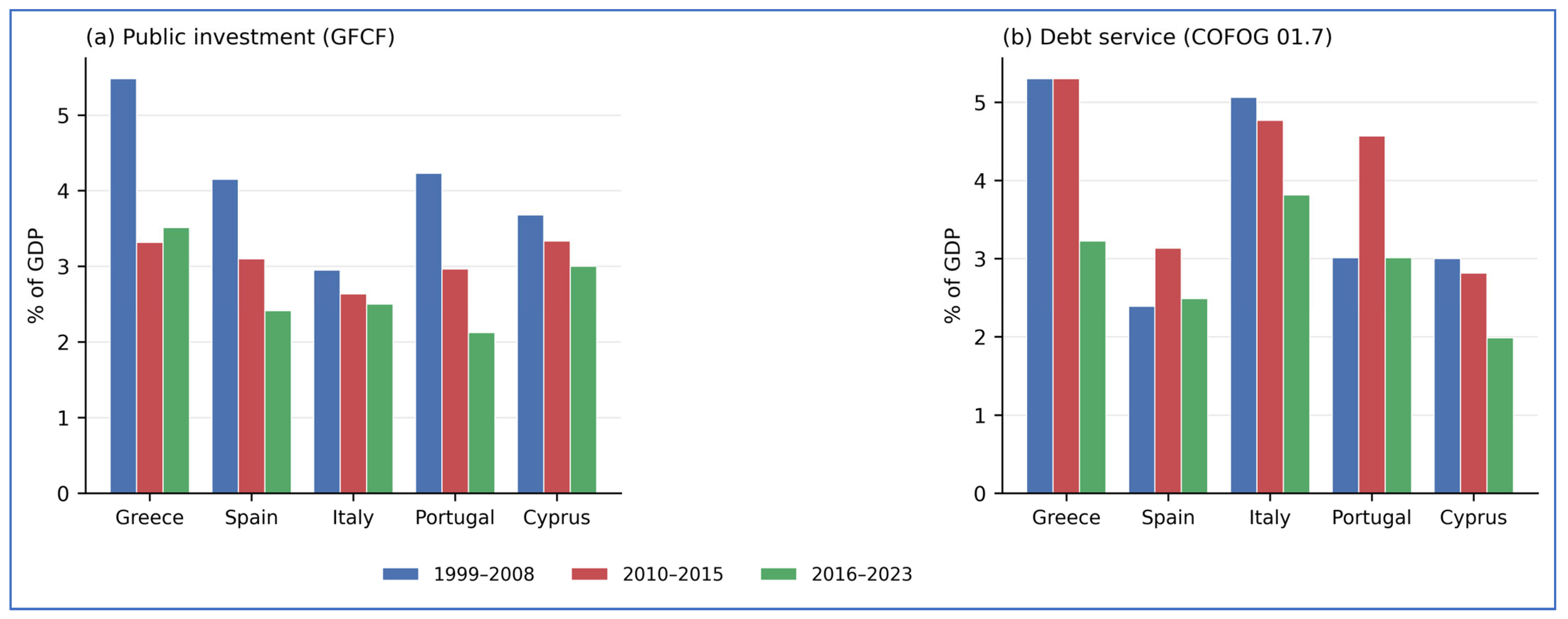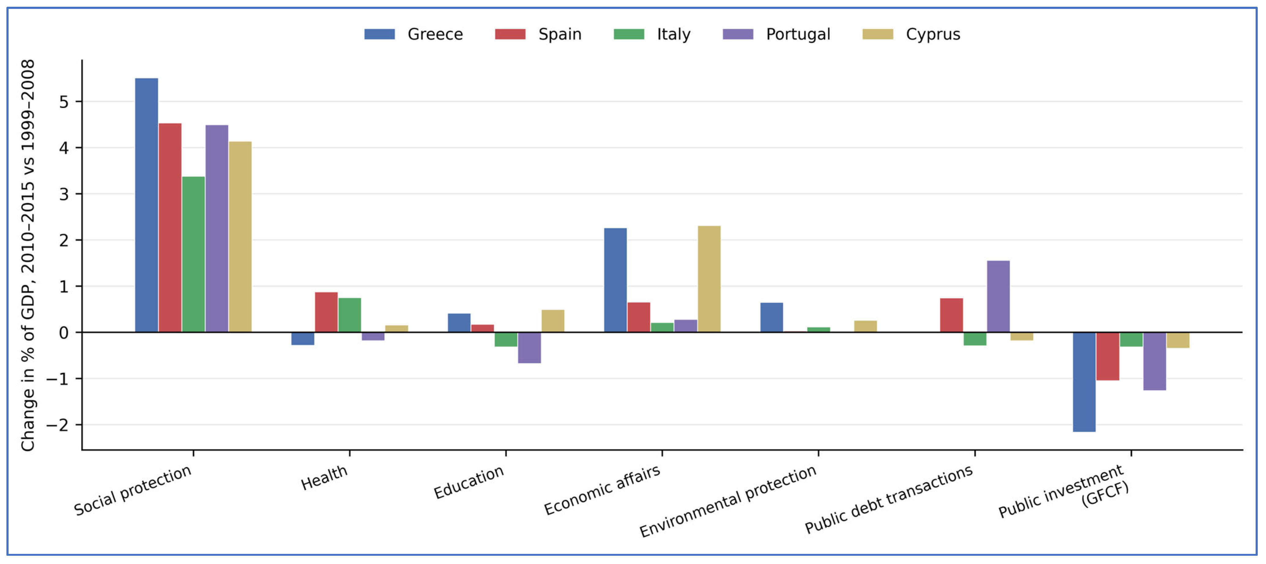Figure 2 and Figure 3 report the results.

The first result is that consolidation in these economies did not reduce the size of the state. Total general government expenditure as a share of GDP rose between the pre-crisis and adjustment periods in every country, by 8.1 percentage points in Greece, 8.0 in Cyprus, 6.9 in Spain, 5.4 in Portugal and 3.2 in Italy. Part of this reflects the denominator, since output contracted sharply, and part reflects the operation of automatic stabilisers. Social protection expenditure rose in all five economies, by between 3.4 and 5.5 percentage points of GDP, as unemployment and pension commitments increased while the tax base contracted.

The second result concerns what gave way. As Figure 3 shows, public investment is the only function that contracted in every country, and by amounts that dwarf the movements elsewhere in the budget. Relative to the pre-crisis average, gross fixed capital formation declined by 39.5 per cent in Greece, 29.9 per cent in Portugal, 25.3 per cent in Spain, 10.7 per cent in Italy and 9.4 per cent in Cyprus. Expressed as a share of total expenditure, investment roughly halved in Greece, from 11.4 to 5.9 per cent, in Portugal from 9.5 to 5.9 per cent, and fell from 10.6 to 6.7 per cent in Spain. The adjustment was therefore not a contraction of the budget but a recomposition of it, in which the forward-looking component was compressed while transfer commitments expanded. This corresponds to the mechanism identified in the literature on the composition of consolidation, in which capital expenditure is compressed because it is politically less costly to postpone than current transfers [66,67].

The third result concerns the debt-service channel. Expenditure on public debt transactions is shown in Figure 2b. During the adjustment period, Greece devoted 5.3 per cent of GDP to debt service against 3.3 per cent to public investment, Italy 4.8 against 2.6 per cent, and Portugal 4.6 against 3.0 per cent. In each of these three economies, the budget therefore transferred more resources to creditors than to capital formation throughout the adjustment years. The Portuguese case is the most direct illustration of the trade-off: debt service rose by 1.6 percentage points of GDP between the pre-crisis and adjustment periods while public investment fell by 1.3 points, so that the increase in the interest burden was of almost the same magnitude as the reduction in capital formation. Debt service has since declined in all five economies, to between 2.0 and 3.8 per cent of GDP, reflecting the low interest-rate environment after 2015 and, in the Greek case, the concessional terms and extended maturities of official lending.

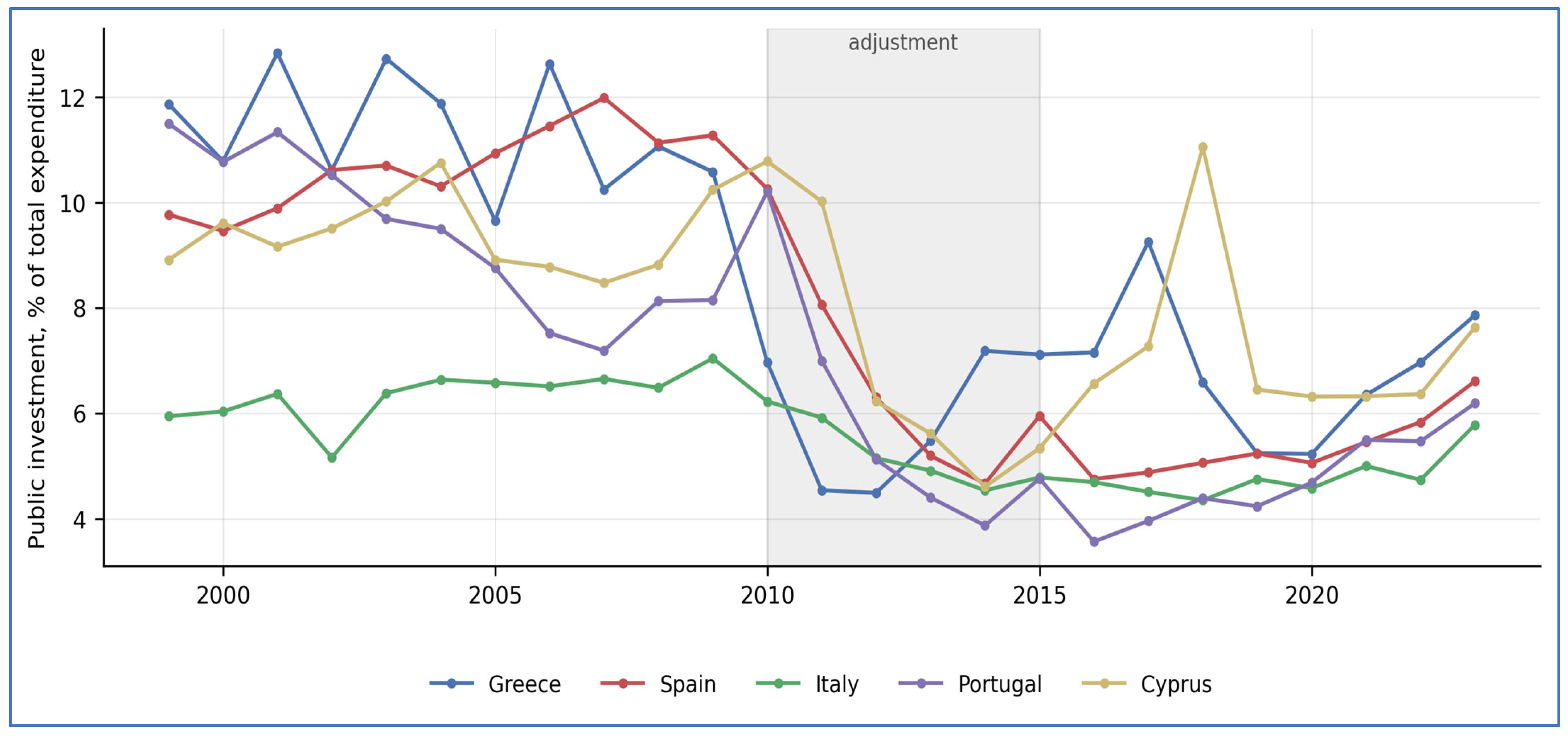
The fourth result is that the compression has not reversed. Figure 4 traces public investment as a share of total expenditure over the full sample. In Spain, Portugal and Italy, investment in the post-adjustment period is lower than during the adjustment itself, at 2.4, 2.1 and 2.5 per cent of GDP respectively, against pre-crisis averages of 4.2, 4.2 and 3.0 per cent. Education expenditure likewise remains below its pre-crisis share of GDP in Portugal, where it fell by 1.8 percentage points, and in Italy. Environmental protection expenditure never exceeded 1.2 per cent of GDP in any country in any period and is essentially unchanged across the sample, so that the fiscal effort directed to the environmental dimension of the Sustainable Development Goals has been small throughout and was not expanded during the recovery.

These findings qualify the interpretation of the adjustment channels reported in Section 3.5. The magnitude of the investment compression is not aligned with the side of the budget that adjusts: Greece, where correction operated weakly through revenue, recorded the largest investment cut, while Cyprus, where correction operated through expenditure, recorded the smallest. What the composition data establish is that public investment was the margin of adjustment in every case, irrespective of which aggregate carried the correction. For sustainable development, this is the operative result. Satisfying the revenue–expenditure condition, or failing to satisfy it, tells us whether the budget was internally consistent; the composition data tell us that the consistency was purchased, in each of these economies, at the expense of the capital formation on which future developmental capacity depends. The comparison with debt service sharpens the point: in the three most indebted economies the adjustment years were ones in which the budget financed past borrowing more generously than future capacity, which is the mechanism by which an unfavourable interest–growth differential translates into a developmental cost.

3.7. Adjustment Capacity Before and After the Crisis

The estimates in Section 3.5 are computed over the full sample and therefore average across two very different fiscal regimes.

Table 12. Error-correction coefficients before and after the sovereign-debt crisis.

Country	Pre-2010: Revenue (t)	Expenditure (t)	Post-2010: Revenue (t)	Expenditure (t)
Greece	−0.159 (−0.92)	0.240 (1.26)	−0.133 (−1.54)	0.252 (2.63)
Spain	0.016 (0.14)	0.075 (2.95)	−0.012 (−0.15)	0.244 (3.90)
Italy	−0.415 (−2.71)	0.001 (0.01)	−0.404 (−3.19)	−0.132 (−1.03)
Portugal	−0.172 (−1.10)	0.262 (1.85)	0.022 (0.28)	0.363 (3.03)
Cyprus	−0.476 (−3.09)	−0.027 (−0.26)	0.063 (0.53)	0.578 (3.28)

Notes: The error-correction term is estimated on the full sample; the conditional models are estimated separately over 1999–2009 and 2010–2023 with seasonal dummies and HAC standard errors. Bold entries denote significance at the five per cent level.

re-estimates the conditional models separately for 1999–2009 and 2010–2023. Three patterns emerge. In Greece and Portugal neither side of the budget responded significantly to disequilibrium before 2010, whereas expenditure-side correction becomes significant afterwards, with coefficients of 0.252 and 0.363. In Spain the expenditure response is present throughout but strengthens from 0.075 to 0.244. In Cyprus the channel switches: revenue carried the correction before the crisis, with a coefficient of −0.476, and expenditure carries it afterwards, at 0.578. Italy alone is unchanged, with a revenue-side correction of −0.415 before and −0.404 after, and no significant expenditure response in either period.

The implication is that adjustment capacity was created rather than merely intensified. In the three economies that entered adjustment programmes without a pre-existing correction mechanism, one emerged during the programme period and has persisted beyond it. This is a more favourable reading of the conditionality period than the causality classifications alone would support, and it is the one respect in which the pre- and post-crisis comparison identifies a durable institutional change rather than a temporary compression of spending.

3.8. Robustness: Revenue and Expenditure as Shares of GDP

The specifications reported above are estimated on the logarithms of nominal revenue and expenditure, which is the form in which the intertemporal budget constraint of Section 1.1 is defined and in which the cointegrating slope carries its Hakkio–Rush interpretation. An alternative and widely used practice expresses both aggregates as shares of nominal GDP.

Table 13. Robustness: analysis with revenue and expenditure expressed as shares of GDP.

Country	ADF rev, Level (p)	ADF Δrev (p)	ADF exp, Level (p)	ADF Δexp (p)	Johansen Trace	Conclusion	β	α Revenue (t)	α Expenditure (t)	Adjusts
Greece	0.655	0.051	0.131	0.000	15.93	Cointegrated	0.612	−0.125 (−2.01)	0.011 (0.11)	Revenue
Spain	0.632	0.036	0.497	0.000	14.25	Not cointegrated	0.066	−0.071 (−0.92)	−0.131 (−1.16)	Neither
Italy	0.708	0.008	0.756	0.000	5.33	Not cointegrated	0.477	−0.054 (−0.69)	0.257 (1.34)	Neither
Portugal	0.499	0.000	0.292	0.000	11.29	Not cointegrated	0.235	−0.230 (−2.54)	−0.188 (−0.84)	Revenue
Cyprus	0.198	0.000	0.330	0.000	18.41	Cointegrated	0.273	−0.267 (−2.77)	0.113 (0.43)	Revenue

Notes: Revenue and expenditure expressed as percentages of unadjusted nominal GDP at current prices (Eurostat, namq_10_gdp). Entries under ADF are p-values; KPSS statistics reject stationarity in levels for all series and fail to reject in first differences. Johansen tests estimated at the lag orders of Table 3; the 5% critical value for the trace statistic is 15.494. β is the cointegrating slope from a dynamic ordinary least squares regression with seasonal terms; in the ratio specification it does not carry the Hakkio–Rush coverage interpretation. Error-correction models estimated with the lag orders of Table 3, seasonal dummies, and heteroskedasticity- and autocorrelation-consistent standard errors. Adjustment is attributed to the side whose error-correction coefficient is correctly signed and significant at the ten per cent level.

reports the principal results on that basis, using unadjusted GDP at current prices so that the numerator and denominator are consistently measured.

Both ratios are integrated of order one in all five economies, in agreement with the level specification: the augmented Dickey–Fuller test fails to reject the unit-root null in levels and rejects it in first differences, while the KPSS statistic rejects stationarity in levels for every series. The remaining results diverge. The Johansen tests identify a cointegrating relationship in Greece and Cyprus rather than in Italy and Cyprus, and the Italian trace statistic falls from 52.51 in levels to 5.33 in ratios. The error-correction estimates attribute the adjustment to revenue in Greece, Portugal and Cyprus, whereas the level specification attributes it to expenditure in Spain, Portugal and Cyprus and to revenue in Italy.

The reason for the divergence is identifiable rather than arbitrary. Expressing both aggregates as shares of a common denominator induces comovement whenever output moves sharply, and the sample contains two such episodes. Output fell substantially in all five economies between 2008 and 2013 and again in 2020, so that both ratios rose without any change in the underlying fiscal aggregates. Since revenue is the more cyclically sensitive of the two, the transformation loads a larger share of the resulting comovement onto the revenue series, which is consistent with the shift of the estimated adjustment toward revenue in three countries. The cointegrating slopes in the ratio specification, which range from 0.07 to 0.61, should for the same reason not be read as coverage ratios in the sense of Hakkio and Rush [12].

We therefore retain the level specification as the baseline, on the grounds that the sustainability condition is defined on levels and that the ratio transformation confounds fiscal behaviour with movements in the denominator during precisely the period of interest. The divergence is nonetheless reported in full, because it constitutes further evidence for the central finding of the paper. A choice between two defensible measurement conventions, holding country, period, data source and estimator constant, alters the cointegration verdict for two economies and the identified adjustment channel for three. This is the same phenomenon documented in Section 4.1 for the choice of causality procedure, and it reinforces the conclusion that fiscal classifications should not be treated as robust properties of the budgets to which they are attached.

4. Discussion

Table 14. Summary of fiscal classifications across methods.

Country	Cointegrated	Bivariate	Trivariate (GDP)	Toda–Yamamoto
Greece	No	Tax-and-spend	Tax-and-spend	Fiscal synchronisation
Spain	No	Tax-and-spend	Tax-and-spend	Spend-and-tax
Italy	Yes	Spend-and-tax	Spend-and-tax	Spend-and-tax
Portugal	No	Tax-and-spend	Spend-and-tax	Institutional separation
Cyprus	Yes	Tax-and-spend	Tax-and-spend	Tax-and-spend

Notes: The table compares fiscal classifications across the three causality procedures. Greece, Spain and Portugal receive different classifications depending on the procedure; Portugal receives a different one under each, while Italy and Cyprus are classified consistently. The table should be read as a demonstration of specification dependence rather than as a settled set of country classifications.

summarises the classifications obtained from each method, and the pattern is one of substantial but not universal sensitivity to methodological choice. Greece moves from tax-and-spend under both Granger specifications to fiscal synchronisation under Toda–Yamamoto. Spain is classified as tax-and-spend by both Granger specifications but as spend-and-tax under Toda–Yamamoto. Portugal is the extreme case, moving from tax-and-spend in the bivariate test to spend-and-tax when output is added and to institutional separation under Toda–Yamamoto, so that each procedure yields a different answer. Italy and Cyprus, by contrast, are classified consistently: Italy as spend-and-tax and Cyprus as tax-and-spend under all three procedures. Three of the five economies therefore receive no stable classification, while two do.

4.1. The Instability of Fiscal Classifications

The central result of this paper is largely negative and should be stated as such. Across three causality procedures applied to identical data, three of the five economies receive different classifications depending on the procedure chosen, and Portugal receives a different classification under each. Only Italy and Cyprus are classified consistently. This is not a caveat attaching to an otherwise clean set of findings; it is the principal finding. Any single-procedure study of these five economies would have produced a definite classification for each, and that classification would have been an artefact of the procedure chosen as much as a property of the underlying fiscal process. The implication for the wider literature is direct: the disagreement between existing studies of the revenue–expenditure nexus need not indicate that they analysed different countries or periods, since studies of the same country and period can disagree purely on method. The two exceptions are informative rather than merely residual. Italy is also the economy whose error-correction channel is stable across every robustness check reported here, retaining revenue-side adjustment in both sub-periods and at every lag order. Where a stable underlying adjustment mechanism exists, the causality procedures agree; where it does not, they diverge. Consistency of classification is therefore not a property of the method but of the budget being classified.

The instability is not, however, uniform across all results reported here. The error-correction estimates of Section 3.5 are considerably more stable than the causality classifications. Re-estimating the conditional models across lag orders from two to six leaves the identified adjustment channel unchanged in Spain, Italy, Portugal and Cyprus in every specification, and in Greece in four of five.

Table 15. Robustness of the adjustment channel across lag specifications.

Country	k = 2	k = 3	k = 4	k = 5	k = 6
Greece	REV	none	REV	REV	REV
Spain	EXP	EXP	EXP	EXP	EXP
Italy	REV	REV	REV	REV	REV
Portugal	EXP	EXP	EXP	EXP	EXP
Cyprus	EXP	EXP	EXP	EXP	EXP

Notes: Entries report the side of the budget whose error-correction coefficient is correctly signed and significant at the ten per cent level, estimated at lag orders k = 2 to 6 with seasonal dummies and heteroskedasticity- and autocorrelation-consistent standard errors.

reports this comparison. The distinction matters for what can legitimately be concluded: statements about which side of the budget responds to disequilibrium rest on estimates that survive changes in specification, whereas statements assigning a country to one of the four hypotheses do not. The country-level interpretation in Section 4.2 is therefore built on the former rather than the latter.

Three substantive lessons follow. First, conditioning on output matters: for Portugal and Cyprus, adding GDP to the information set changes the fiscal classification, and for Cyprus it weakens the surviving channel from the one per cent to the ten per cent level, confirming that bivariate revenue–expenditure tests are vulnerable to omitted-variable bias because national income drives both aggregates. Second, the treatment of non-stationarity and cointegration matters: the Toda–Yamamoto procedure, which is valid irrespective of integration properties, reclassifies Greece and Spain relative to the standard Granger tests, indicating that conventional tests applied to I(1) fiscal data can mislead. Third, structural breaks matter, and the manner in which the relationship changed can be specified rather than merely asserted. Three changes occurred together. The location of the breaks identifies the timing: the Quandt–Andrews tests place the revenue-equation break in 2008 or 2009 for Greece, Spain and Portugal, at the point at which the revenue base contracted, while the expenditure-equation breaks are later and more dispersed, between 2011 and 2019, reflecting the country-specific timing of the adjustment programmes. The direction of change is given by the sub-period estimates in Section 3.7: in Greece and Portugal no side of the budget corrected significantly before 2010, and expenditure-side correction became significant afterwards; in Spain the existing expenditure response strengthened threefold, and in Cyprus the adjusting side switched from revenue to expenditure. The content of the change is given by the composition evidence in Section 3.6: the recomposition of spending away from public investment and toward social protection, with debt service exceeding capital formation in the three most indebted economies. Taken together, the crisis did not simply add noise to an existing relationship. It created correction mechanisms where none had operated, altered which instrument performed the correction in one case, and changed the composition of the expenditure through which the correction was delivered.

The divergences are not arbitrary, and each has a counterpart in the fiscal history of the country concerned. In Greece, the bivariate and trivariate procedures point to tax-and-spend while the Toda–Yamamoto procedure indicates synchronisation. Greece is also the economy with no cointegrating relationship and the most pronounced parameter instability, with significant breaks in both the revenue and the expenditure equation. Because the Toda–Yamamoto procedure is estimated in levels, it retains the low-frequency comovement generated by the successive programme packages, in which revenue and expenditure measures were legislated together, whereas the differenced specifications capture only the shorter-run sequencing in which revenue measures were typically implemented first. In Spain, the bivariate result of tax-and-spend reverses to spend-and-tax under Toda–Yamamoto. The Spanish revenue series contains the largest single exogenous movement in the sample, the collapse of construction-related receipts after 2008, which dominates the differenced data and gives revenue apparent leading power; in levels, where that episode is one feature of a longer series rather than the dominant source of variation, the expenditure side is identified as leading. Italy, by contrast, is classified as spend-and-tax under all three procedures. It is also the economy whose error-correction channel is stable across every robustness check reported here, retaining revenue-side adjustment in both sub-periods and at every lag order. Where a stable underlying adjustment mechanism exists, the procedures agree. In Portugal the direction reverses once GDP enters, from tax-and-spend to spend-and-tax, and the Toda–Yamamoto procedure finds neither direction significant, so each procedure yields a different answer. Portugal is also the economy in which programme measures were repeatedly annulled and re-specified, and in which the revenue-equation break is significant only at the earlier of the two dates tested. In Cyprus the tax-and-spend classification survives all three procedures but weakens substantially when output is conditioned upon, from the one per cent to the ten per cent level, which suggests that part of the apparent comovement in this small open economy is a common response to the output cycle. The general point is that the sensitivity of the classifications is informative about the underlying fiscal processes: procedures diverge most for the economies whose fiscal series were most disturbed by discrete events, and least for Italy, whose budget adjusted through a stable revenue-side mechanism throughout. Cyprus is consistent for a different reason: its short and volatile series is dominated by the single episode of 2013, which the three procedures identify alike, rather than by a stable adjustment mechanism.

4.2. Country Interpretation

Read together with the fiscal histories set out in Section 2.2, the error-correction estimates in Table 11 are more informative than the causal classifications alone.

The Italian result is the clearest. Revenue carries the adjustment, with an error-correction coefficient of −0.472 and a t-statistic of −4.17, while expenditure does not respond significantly. This corresponds closely to the historical record: Italy sustained primary surpluses through most of the sample and pursued consolidation predominantly through taxation, notably the property-tax and value-added-tax measures of 2011 and 2012. It also corroborates Legrenzi and Milas [15], who find within a nonlinear error-correction framework that the burden of correcting Italian budgetary disequilibria falls on the average tax rate, with government spending weakly exogenous. That two different specifications, applied to different sample periods, identify the same adjustment channel strengthens confidence in the finding.

Spain presents the opposite configuration. Expenditure adjusts, with a coefficient of 0.210 and a t-statistic of 4.83, while revenue does not. This is consistent with a fiscal deterioration whose origin was a cyclical collapse in construction-related revenue rather than a discretionary loosening. Because the revenue shock was largely outside the government’s control, adjustment operated through the expenditure side, and Spain’s subsequent recovery has been accompanied by a passive revenue rebound rather than by a sustained discretionary revenue effort. The finding also indicates why the Spanish cointegration result is fragile: an exogenous revenue break of this magnitude weakens any stable long-run relationship estimated across it.

Portugal and Cyprus display the same expenditure-led pattern, with coefficients of 0.342 and 0.477 respectively. In both cases the adjustment was programme-driven and concentrated in a short period, and in both the programme design placed primary weight on expenditure measures. The larger Cypriot coefficient is consistent with the compressed and severe nature of the 2013 adjustment. In Portugal, the annulment of several measures by the Constitutional Court means that the estimated adjustment reflects a process that was repeatedly interrupted and re-specified, which may account for the absence of a stable long-run relationship in Table 4 despite significant short-run expenditure adjustment.

Greece is the case in which no side of the budget adjusts reliably. The revenue coefficient is negative but significant only at the ten per cent level, and expenditure does not respond. This is the econometric counterpart of the historical record: three successive programmes, repeated revisions of fiscal targets, and the absence of a cointegrating relationship reported in Section 4.2. The scale of Greek adjustment was larger than anywhere else in the sample, but it did not produce a stable equilibrium relationship between the two aggregates within the period examined.

Two general points follow. First, the side of the budget that adjusts is closely connected to the origin of the imbalance rather than to any general property of the fiscal system, which is an argument against uniform prescriptions across the periphery. Second, the causal classifications in Table 5, Table 6 and Table 7 are least stable precisely for those economies, Spain and Portugal, whose revenue or expenditure series were most disturbed by discrete events during the sample. Method sensitivity is therefore not only an econometric artefact; it is partly a reflection of genuine structural change in the underlying fiscal processes.

These findings help explain why the empirical literature on the revenue–expenditure nexus has reached such mixed conclusions. If the classification of a given country depends on whether output is conditioned upon, on how non-stationarity is handled, and on whether structural breaks are accommodated, then studies differing in these respects will naturally reach divergent conclusions even for the same country and period. The appropriate response is not to select one procedure and present its classification as the finding, but to estimate the alternatives and report them together, so that the reader can see which conclusions hold across specifications and which do not. On this reading the fiscal relationship is properly described as specification-dependent and regime-dependent rather than as a fixed attribute of a country. For the euro-area periphery specifically, the appropriate conclusion is not that any of these economies belongs to one of the four categories, but that the categories themselves are too fragile to carry the weight that the policy literature places on them. What survives the change in procedure is the adjustment evidence: revenue-led correction in Italy, expenditure-led correction in Spain, Portugal and Cyprus, and no reliable correction in Greece.

5. Conclusions

This paper has examined the causal relationship between government revenue and expenditure in five Southern European economies over 1999–2023, testing the four hypotheses of the revenue–expenditure nexus within a multiple-test research design. The central finding is that fiscal-causality classifications are not robust to methodological choices: they depend on whether output is included as a conditioning variable, on whether the causality test accommodates the integration and cointegration properties of the data, and on whether structural breaks are taken into account. Across the three causality procedures, three of the five economies receive different classifications, and only Italy and Cyprus are classified consistently. The structural-break analysis shows that the revenue–expenditure relationship was significantly altered around the onset of the crisis, with the evidence strongest when the break is tested at 2009Q1.

For policymakers, the results bear on the design of national fiscal rules, and three points follow. The first concerns the relationship between national rules and the European framework. The country-specific rules proposed here are not alternatives to the common requirements but supplements to them. Since the 2024 reform of the economic governance framework, the operational anchor for each Member State is a country-specific net expenditure path embedded in a medium-term fiscal-structural plan, agreed with the Commission and the Council and monitored through a control account [66]. The framework already accommodates national differentiation; the question is what each national plan should contain, and it is here that evidence on the adjustment channel is informative.

The second point concerns the choice of instrument. An expenditure rule can only bind where expenditure is the margin that responds to budgetary disequilibrium. The evidence in Table 15 indicates that this condition is satisfied in Spain, Portugal and Cyprus, and in Greece since 2010, where the expenditure-side error-correction coefficients are significant and, in three of the four, have strengthened over time. In these economies the net expenditure path is well matched to the observed behaviour of the budget. Italy is the exception that matters: revenue carries the correction in both sub-periods, with a coefficient near −0.4, while expenditure shows no significant response in either. A rule anchored exclusively on net expenditure therefore targets, in the Italian case, the side of the budget that has historically not adjusted. The implication is not that Italy should be exempt from the common framework, but that its medium-term plan should be complemented by commitments on the revenue side, where the adjustment has in practice occurred.

The third point concerns economies in which neither side reliably corrects, or in which both do. Where the two aggregates are jointly determined, an expenditure ceiling alone permits the correction to be undone through discretionary revenue measures, and a revenue rule alone permits the reverse. In such cases the binding instrument is an offsetting requirement: any measure that reduces revenue or raises expenditure must be matched by a compensating measure elsewhere in the budget, so that the rule applies to the balance rather than to either component. This is the appropriate design for Greece, where the revenue response remains statistically weak even after 2010 and the expenditure response, although significant, coexists with the largest cointegration failure in the sample.

A final consideration cuts across all three. The composition evidence in Section 3.6 shows that adjustment in these economies fell on public investment rather than on the size of the budget. Because the net expenditure indicator is defined net of interest and of certain EU-funded items but not of nationally financed capital spending, a path calibrated on aggregate expenditure growth leaves the investment component as the easiest margin of compliance. National plans should therefore protect capital expenditure explicitly, whether through a golden-rule provision or through the investment-linked extension of the adjustment period that the framework already permits [67]. Otherwise, the rules will secure budgetary consistency by the same mechanism that produced it in 2010–2015, namely the compression of the public capital stock.

These considerations bear directly on the practical question of how a budget can be planned toward balance in economies carrying a heavy interest burden. Three implications follow from the expenditure structure documented in Section 3.6. First, the discretionary margin is far smaller than headline expenditure suggests. During the adjustment years, interest payments and social protection together accounted for 50.1 per cent of total expenditure in Italy, 46.1 per cent in Portugal, 45.8 per cent in Greece and 44.6 per cent in Spain, and these proportions have barely changed since. Roughly half of the budget in these economies is committed before any planning decision is taken, since interest is contractually fixed in the short run and social transfers are governed by entitlement rules rather than annual appropriation. A consolidation target expressed as a percentage of total expenditure therefore implies an adjustment of approximately twice that magnitude on the programmable remainder, which is the arithmetic that produced the compression of investment described earlier.

Second, it follows that expenditure planning should operate on primary expenditure rather than on the total. The net expenditure indicator adopted under the reformed European framework already excludes interest, which is appropriate, but national planning documents should make the same distinction explicit and set multi-annual ceilings on primary current expenditure rather than annual targets for the overall balance. An annual balance target transmits interest-rate shocks directly into the programmable budget, whereas a primary-expenditure ceiling insulates planning from movements in debt service that no government can control within the budget year.

Third, the management of the debt-service burden is itself a fiscal-planning instrument rather than a constraint to be accepted. The Greek experience is instructive: debt service fell from 5.3 per cent of GDP during the adjustment years to 3.2 per cent afterwards, not because the debt stock declined but because official lending at extended maturities and fixed rates reduced the effective interest cost and insulated it from market conditions. Portugal and Italy recorded comparable reductions, to 3.0 and 3.8 per cent. Extending maturity and increasing the fixed-rate share of the stock therefore widens the programmable margin in a way that no expenditure rule can, and should be treated as complementary to the rules rather than separate from them. For governments in this position, the sequence that follows from our results is to secure the debt-service profile first, protect capital expenditure explicitly second, and apply the correction to the remaining primary current expenditure third, using the instrument that the evidence in Section 3.5 identifies as the responsive one in that country.

For sustainable development, the implication is more pointed. Greece and Portugal are the economies in which the intertemporal budget constraint is not satisfied, and Spain occupies an intermediate position in which the evidence depends on specification. In none of the three does a robust long-run relationship discipline the budget. Without that anchor, the fiscal space available for the sustained public investment that the Sustainable Development Goals require depends on market conditions rather than on domestic fiscal capacity. Restoring a stable long-run relationship between revenue and expenditure is therefore a precondition for the developmental use of the budget rather than a competitor to it. The same evidence cautions against uniform fiscal rules across the periphery, since the countries differ both in whether the constraint binds and in which side of the budget adjusts. This inference is necessarily partial. Greece and Italy carried debt ratios well above one hundred per cent of GDP for much of the sample, and for such economies the binding constraint on fiscal space is often the interest–growth differential and the debt-service burden rather than the revenue–expenditure relationship alone. The results presented here identify a necessary condition that was not met in Greece and Portugal; they do not quantify the fiscal space available to any of the five governments.

The composition evidence sharpens this point. In all five economies, the adjustment fell on public investment rather than on the size of the budget, and in three of them investment remains below its crisis-period level. In Greece, Italy and Portugal, the interest burden absorbed a larger share of the budget than capital formation during the adjustment years, so that the interest–growth differential operated not only on the debt ratio but on the composition of spending. Fiscal rules that target aggregate balances without distinguishing capital from current expenditure therefore risk securing budgetary consistency at the cost of the public capital stock, which is the channel through which fiscal policy contributes most directly to the Sustainable Development Goals.

Several limitations bound these conclusions and suggest avenues for further work. The framework is confined to the two aggregate sides of the budget. A fuller assessment of fiscal sustainability would model the dynamics of the debt-to-GDP ratio directly, incorporating the primary balance, the effective interest rate on public debt, nominal growth and the interest–growth differential, and would allow the debt-service channel to feed back into both revenue and expenditure. Extending the analysis in that direction, in the manner of the debt-dynamics literature, is the most promising next step and would allow the necessary condition examined here to be embedded within a sufficient one.

The analysis covers five economies and a single quarterly dataset; extending it to the full euro area would allow the regularities to be assessed against a wider set of fiscal institutions. The causality tests are linear, and non-linear or regime-switching methods might capture the crisis-driven dynamics more directly than the structural-break tests employed here. Semiparametric estimators of policy effects offer one such route [68]. Finally, a fourth causality procedure could be added for the economies in which a cointegrating relationship is identified. Where revenue and expenditure are cointegrated, as they are in Italy and Cyprus, Granger causality can be tested within a vector error-correction model, in which the direction of causality is inferred jointly from the lagged differences and from the significance of the error-correction term itself. This distinguishes short-run causality, operating through the lagged differences, from long-run causality, operating through the adjustment to disequilibrium, a distinction that neither the differenced Granger tests nor the level-based Toda–Yamamoto procedure can make. We report the error-correction coefficients separately in Section 3.5 rather than embedding them in a causality test, so the two components are estimated but not combined into a single classification. Doing so would extend the comparison of procedures that is the subject of this paper to a fourth method, and would be a natural next step. These extensions notwithstanding, the evidence presented here makes a clear methodological point: in the empirical analysis of the revenue–expenditure nexus, the conclusion one reaches is conditional on how one asks the question.