Article

A Carbon Efficiency Traceability Monitoring Model for Discrete Manufacturing Workshops with Event Concurrency

1
Key Laboratory of Metallurgical Machine and Control Technology, Ministry of Education, Wuhan University of Science and Technology, Wuhan 430081, China
2
Hubei Key Laboratory of Mechanical Transmission and Manufacturing Engineering, Wuhan University of Science and Technology, Wuhan 430081, China
3
Academy of Green Manufacturing Engineering, Wuhan University of Science and Technology, Wuhan 430081, China
*
Author to whom correspondence should be addressed.
Sustainability 2026, 18(16), 8363; https://doi.org/10.3390/su18168363
Submission received: 17 July 2026 / Revised: 7 August 2026 / Accepted: 12 August 2026 / Published: 14 August 2026

Abstract

Carbon efficiency, measuring effective output per unit of carbon emissions, is vital for managing low-carbon workshops and advancing sustainable manufacturing. However, production processes often face concurrent discrete events (e.g., equipment failures, parameter adjustments) and numerous emission factors with complex relationships, making it hard to identify dominant factors and event impact degrees, thus lacking direction for operation and maintenance decisions. This paper proposes a deductive monitoring model to analyze carbon efficiency changes under event concurrency. First, for traceability, a multi-resolution enhanced carbon efficiency information transfer network is proposed. It classifies emission factors into time-driven and event-driven accounting, and under the Parallel Discrete Event System Specification framework, adopts a multi-resolution approach with high- and low-resolution models for hierarchical aggregation from equipment to workshop, establishing a traceability path to specific factors. Second, for unclear impact degrees, a dynamic monitoring model for concurrent events is designed. A state-driven dynamic carbon efficiency accounting method automatically settles upon equipment state switching, and a rule-driven priority deduction strategy enables independent accounting of each event’s impact degrees in a determined order. A case study on a machine tool spindle production workshop validates the proposed model. Under baseline conditions, the relative accounting errors for 8 h cumulative carbon emissions and effective output are approximately 1.05% and 0.89%, respectively. In concurrent event scenarios, the model achieves deterministic trajectory reproducibility across 30 independent deduction runs and enables independent impact-degree decomposition, whereas traditional discrete event simulation exhibits trajectory ambiguity. Furthermore, testing under 42 multi-parameter perturbation combinations demonstrates traceability path integrity and accurate root-cause localization, delivering a transparent and reliable quantitative basis for low-carbon maintenance decisions.

1. Introduction

Sustainable manufacturing is essential for global industrial decarbonization and achieving net-zero targets, driving manufacturing systems toward resource-efficient and low-carbon operations [1,2]. As a major sector of sustainable manufacturing, discrete manufacturing encompasses key industries such as automotive components and machine tool fabrication, involving multi-process and multi-machine operations [3,4]. Under low-carbon constraints, discrete manufacturing workshops must control total carbon emissions while improving carbon efficiency—defined as the ratio of effective physical output to total carbon emissions [5]. A higher carbon efficiency indicates that more qualified workpieces are produced per unit of carbon emissions [6]. Consequently, carbon efficiency monitoring plays a critical role in shop-floor low-carbon management.
However, the production process in discrete manufacturing workshops is frequently affected by multiple types of discrete events, such as equipment failures, maintenance operations, parameter adjustments, and order changes. The dynamic changes in carbon emissions are frequent and complex. In actual operation and maintenance, multiple types of discrete events often occur in parallel, such as an unexpected breakdown on one machine tool occurring simultaneously with a cutting parameter adjustment on another. Carbon efficiency fluctuations are usually the result of the superimposed effects of multiple events. It is difficult for monitoring models to accurately determine the specific cause of each fluctuation. It remains unclear which carbon emission factors have changed abnormally. The impact degrees of different events cannot be distinguished. This leaves maintenance decisions without a reliable basis and may lead to excessive or insufficient maintenance. Therefore, a monitoring method is urgently needed. This method must be capable of attributing and quantitatively analyzing carbon efficiency fluctuations under multi-event concurrent conditions.
Existing carbon efficiency monitoring methods mainly include statistical analysis [7,8], machine learning prediction [9], and virtual simulation [10]. Statistical analysis methods offer transparent calculations and strong interpretability. However, their accuracy drops significantly when facing discrete events not covered by historical data. Machine learning methods can learn complex mapping relationships between carbon emissions and output from large amounts of data. However, the internal mechanisms of these models are opaque. This makes it difficult to reveal the causal chain of carbon efficiency changes and to effectively guide the adjustment of maintenance strategies. Virtual simulation technology simulates workshop operation dynamics through model deduction. It can adapt to various event changes and offers a certain degree of interpretability and flexibility. Nevertheless, its application in carbon efficiency monitoring still has two shortcomings. First, most existing simulation models have not established systematic associations between carbon emission factors, equipment states, and production events. This makes it difficult to trace carbon efficiency fluctuations back to specific carbon emission factors. Second, when multiple events occur concurrently, traditional discrete event simulation struggles to obtain deterministic deduction results under uncertain event sequences. The impact degree of each event cannot be effectively distinguished. This leads to insufficient interpretability of carbon efficiency changes.
To address these limitations, this paper proposes a multi-resolution enhanced carbon efficiency traceability monitoring model based on the Parallel Discrete Event System Specification (PDEVS) framework. The major research contributions of this work are twofold:
(1)
Establishing a multi-resolution enhanced carbon efficiency information transfer network to overcome the broken traceability in existing models. Existing approaches lack systematic coupling among emission factors, equipment states, and discrete events, while treating all data at an undifferentiated granularity. To bridge this gap, this network classifies carbon emission factors into time-driven and event-driven categories, constructing high-resolution equipment atomic models and low-resolution cell/workshop coupled models within the PDEVS framework. By coordinating upward aggregation of event information packets (InfoPkt) and downward mapping of impact degrees, it provides a transparent, three-level traceability path from workshop-level macro fluctuations down to specific equipment and root-cause emission factors.
(2)
Designing a dynamic carbon efficiency monitoring model for event concurrency to resolve trajectory ambiguity in discrete event simulation. Traditional simulation models suffer from execution path uncertainty under concurrent events, making it difficult to obtain deterministic trajectories or isolate individual event impacts. To resolve this ambiguity, a state-driven dynamic settlement mechanism is integrated with a rule-driven priority deduction strategy. Equipment state switches automatically trigger incremental carbon settlement, while manufacturing operation rules are formalized into a three-level event priority system and internal precedence principles. This ensures a deterministic and reproducible carbon efficiency trajectory under concurrent scenarios, enabling independent quantitative decomposition of each event’s impact degree to guide targeted maintenance decisions.
The paper is structured as follows: Section 2 reviews related work. Section 3 presents the method framework. Section 4 elaborates on the multi-resolution enhanced carbon efficiency information transfer network. Section 5 introduces the dynamic carbon efficiency monitoring model for event concurrency. Section 6 uses a machine tool spindle machining workshop as a case study to verify the effectiveness of the proposed method. Section 7 concludes the paper and discusses future research directions.

2. Literature Review

Carbon efficiency monitoring in discrete manufacturing workshops deals with a multi-level complex system. Equipment, cells, and workshops operate at their respective levels, yet they are coupled through material flow and carbon emission transfer. Describing such a system requires answering two fundamental questions. First, what carbon emission factors constitute carbon efficiency, and how are these factors related? Second, how does carbon efficiency change over time when driven by discrete events? The former corresponds to the information modeling of carbon efficiency. The latter corresponds to the analysis of the carbon efficiency change process. Existing research has developed along these two main lines. Analyzing the shortcomings of current studies in these two aspects can provide a basis for the research method and technical route of this paper.

2.1. Research Status of Carbon Efficiency Information Modeling

Carbon efficiency information modeling aims to clarify what carbon emission factors constitute carbon efficiency, how these factors are related, and how they are aggregated upwards to form hierarchical indicators. It is the foundation for carbon efficiency calculation and traceability.
In terms of carbon efficiency factor identification, research focuses on determining which factors influence carbon efficiency and how to incorporate them into a unified accounting framework. For example, Li et al. [11] integrated material, energy, and information flows for process-level evaluation in electronic manufacturing. Process parameters like cutting speed and feed rate were leveraged by Yi et al. [12] for low-carbon CNC machining optimization. Further expanding factor scopes, Zheng et al. [13] correlated product structural features with production batch combinations in casting processing, while Zhang et al. [14] utilized production, status, and consumption data within a digital twin model for real-time workshop emission assessment.
In terms of hierarchical modeling, research focuses on how to aggregate factor accounting results from the equipment layer upwards to form cell-level and workshop-level carbon efficiency indicators. For instance, Zhang and Ji [15] established a multi-source data framework to evaluate carbon indicators across machine, workpiece, and workshop levels. Du et al. [16] proposed a four-layer information architecture encompassing objectives, measures, processes, and support systems. Meanwhile, Li et al. [17] and He et al. [18] structured carbon accounting into multi-tier models (spanning equipment, part, product, line, and workshop levels) to track carbon footprints systematically from process to workshop scales.
The above studies have identified rich carbon emission factors and established hierarchical evaluation frameworks. However, a problem remains in the information modeling approach. They fail to differentiate the recording granularity based on the characteristics of different carbon emission factors. Specifically, emissions from electricity and cutting fluid consumption accumulate continuously with equipment operation status. They need to be tracked and settled step-by-step according to the rhythm of status switches. Emissions from tool replacement and material input are triggered only at specific moments. They only need to be recorded when the event occurs. Existing research treats these two types of factors at the same information granularity. When status switches and discrete events overlap, the settlement timing of the two types of emissions is mixed together. This makes it difficult to precisely align the time points of carbon efficiency changes with production activities, leading to traceability difficulties.
Furthermore, in hierarchical modeling, this undifferentiated processing causes confusion in hierarchical functions. The equipment level should assume the function of step-by-step tracking. The cell and workshop levels should only focus on aggregation trends. However, existing models maintain no difference in information granularity across levels. Uploading all detail data in full causes redundancy. Meanwhile, a downward trace from aggregated indicators to detailed data lacks a mapping path. The traceability path is thus interrupted.
Multi-resolution modeling provides a solution to the above problems [19,20]. Its core idea is to describe system behavior according to the information granularity requirements of each level. In carbon efficiency monitoring, the equipment level can adopt two recording mechanisms simultaneously. For time-cumulative emissions, continuous settlement is performed according to status rhythms. For event-driven emissions, recording is performed only when triggered. The alignment of the two types of settlement moments is achieved through a unified timeline. The cell and workshop levels abstract the high-resolution details of the equipment level into low-resolution carbon efficiency trends through aggregation mapping. They also retain the traceability path from aggregated indicators to original records. This eliminates data redundancy while ensuring a closed traceability path. However, how to coordinate these two carbon efficiency recording mechanisms within the equipment-level model and build an adapted traceability method remains a question for further study.

2.2. Research Status of Carbon Efficiency Change Process

Research on the carbon efficiency change process aims to analyze the dynamic evolution of carbon efficiency driven by discrete events. It focuses on how carbon emissions and output respond to various events over time. Existing methods can be divided into two categories: discrete time-step models and discrete event sequence models.
Discrete time-step models collect data at fixed time steps and analyze the comprehensive impact of multiple events within a period. For example, Zhang et al. [21] utilized real-time data to predict workshop energy consumption under equipment status switches and parameter adjustments. Similar time-step approaches, such as digital twins for progress prediction (Qian et al. [22]), coupled map lattice models for disturbance propagation (Li et al. [23]), and parallel GRU networks for delay bottleneck detection (Fang et al. [24]), demonstrate the efficacy of time-step mechanisms in workshop dynamics. Although these studies do not directly output carbon emissions, their underlying modeling mechanisms are fully consistent with discrete time-step models oriented toward carbon efficiency. Most existing digital twin-based carbon monitoring methods follow this time-step paradigm; they can reflect the overall trend but cannot attribute fluctuations to individual events. However, because they do not explicitly characterize the action process of individual events, it is difficult to attribute changes to specific events when carbon efficiency fluctuates. They cannot support precise traceability.
Discrete event sequence models process data input in an event-driven manner. They deduce the dynamic changes of system states and carbon emissions by maintaining an event sequence, thereby offering enhanced process interpretability compared to time-step models [25]. Based on this mechanism, Wang and Choi [26] integrated stochastic lot-sizing with event sequencing to analyze dynamic trade-offs between profit and carbon emissions. Cao and Li [27] applied hybrid Petri nets to simulate dynamic carbon efficiency under operational events such as machine failures and tool degradation. To handle complex event dynamics, Zhou et al. [28] constructed temporal snapshot networks to evaluate machine loads driven by progressive and sudden event sequences. Similarly, Cai et al. [29] developed a proactive digital twin model to track system state changes under equipment anomalies and material shortages. Although these works do not directly account for carbon emissions, their event-driven deduction mechanisms are fully consistent with discrete event sequence models oriented toward carbon efficiency. They can also track system state changes along the event occurrence sequence, thereby providing a methodological basis for the dynamic traceability of carbon efficiency.
However, discrete event sequence models face a key challenge when handling concurrent events: the distortion of carbon accumulation rates caused by arbitrary randomization of event ordering. In discrete manufacturing workshops, events such as material replenishment for multiple devices, fault maintenance, parameter adjustments, and replacement operations often occur concurrently. If the execution sequence of these concurrent events relies on random or arbitrary ordering rather than systematic manufacturing rules, the recorded start and end times of equipment states will be misaligned. Since time-driven carbon emissions (e.g., electricity and cutting fluid consumption) accumulate strictly based on the exact duration of each state, this misalignment directly distorts the carbon accumulation windows. Consequently, it becomes highly challenging to independently and accurately isolate the carbon impact of individual concurrent events. This arbitrary randomization renders the carbon efficiency monitoring trajectory ambiguous, and it struggles to provide a unique and credible basis for maintenance decisions.
Parallel Discrete Event System Specification (PDEVS) [30,31] provides a formal basis for the deterministic handling of such concurrent events. Particularly in multi-resource manufacturing concurrency, PDEVS performs significantly better than standard DEVS. While standard DEVS forces the sequential processing of simultaneous events across different resources, often leading to tie-breaking ambiguities, PDEVS utilizes a robust parallel transition handling capability that collects all simultaneous events at the exact same time step. Combined with its explicitly defined structured Select function, PDEVS can specify a deterministic processing order for this concurrent event set, resolving ambiguity in concurrent deduction at the mechanism level and ensuring the unique reproducibility of the trajectory. Existing PDEVS applications in manufacturing treat carbon emissions merely as a statistical indicator, lacking targeted architectural designs for carbon emission traceability and event impact decomposition. However, when applying PDEVS to carbon efficiency monitoring, a question remains for further study—specifically, how to design a deterministic concurrent event deduction strategy for the engineering practice of multi-event concurrency in discrete manufacturing workshops. This strategy should enable the independent accounting of the impact degrees of each event and ensure a uniquely reproducible carbon efficiency trajectory.

3. Method Framework

The overall framework of the proposed carbon efficiency traceability monitoring model is shown in Figure 1. The model takes sequential discrete events and the initial system state as inputs. Through carbon efficiency information modeling and concurrent event deduction, it outputs a dynamic and traceable carbon efficiency evolution trajectory. The model construction consists of two core parts.
(1)
Multi-resolution enhanced information transfer network. This part assumes the functions of static organization and hierarchical association of carbon emission factors. Carbon emission factors are divided into time-driven and event-driven types according to the settlement mechanism. A quantitative association between the carbon efficiency calculation formula and each factor is established. Within the PDEVS coupled model framework, a three-layer information transfer structure is constructed, with the equipment level as the high-resolution layer and the cell and workshop levels as the low-resolution layers. In terms of data aggregation and monitoring, the equipment atomic model reports carbon emission and output increments through InfoPkt at each state switch. These are aggregated step-by-step from the cell level to the workshop-level carbon efficiency. In terms of anomaly tracing and attribution, when abnormal fluctuations in carbon efficiency occur, maintenance personnel can trace down the path of workshop, cell, equipment, and factor to locate the dominant equipment and the triggering event. This network provides a structured information flow for carbon efficiency monitoring and traceability.
(2)
Dynamic carbon efficiency monitoring model for event concurrency. This part assumes the functions of dynamic carbon emission deduction and concurrent event processing. Inside the equipment atomic model, a state-driven dynamic carbon efficiency settlement method is designed. It automatically completes carbon emission settlement with each equipment state switch. This ensures that every change point on the carbon efficiency curve has a precise timestamp and an event cause. At the deduction engine level, a rule-driven priority deduction strategy for concurrent events is designed. Based on workshop operation specifications, the event response logic is formalized into a three-level event priority and an internal priority principle. This effectively reduces the uncertainty of results when multiple events are concurrent and improves the determinism and reproducibility of the carbon efficiency monitoring trajectory.
To establish mathematical rigor and reproducibility, the entire monitoring system is formally encapsulated into a multi-resolution PDEVS structure. The base tier consists of equipment atomic models, formally specified as M = X , Y , S , t a , δ i n t , δ e x t , δ c o n , λ . Here, X and Y are the input and output event sets, S captures the dynamic state variables, t a is the time advance function, δ functions govern the internal, external, and confluent state transitions, and λ is the output function. These atomic models are integrated into cell and workshop coupled models, specified as N = X , Y , D , M d d D , E I C , E O C , I C , S e l e c t . Here, D is the index set of sub-models, M d represents the sub-models, S e l e c t determines the processing order for concurrent events, and the message-passing protocol is strictly defined by the coupling interfaces: Internal Coupling ( I C ) channels route the standardized event packets (InfoPkt) generated by λ upward for aggregation, while External Input Coupling ( E I C ) routes control commands downward and External Output Coupling (EOC) transmits aggregated outputs upward.
The model operation is directly driven by the PDEVS main loop algorithm. At each simulation time, concurrent events are collected; scheduled according to the priority strategy (the Select mechanism), triggering state transitions and carbon emission settlement in atomic models; and aggregated step-by-step along the coupling interfaces. The information transfer network defines the factor composition, hierarchical association, and data flow direction of carbon efficiency, providing a static definition framework for traceability. The dynamic monitoring model defines how carbon emissions change in response to events and how concurrent events are processed, providing a dynamic operation mechanism for deduction.

4. Multi-Resolution Enhanced Carbon Efficiency Information Transfer Network

To achieve fluctuation traceability of carbon efficiency, two fundamental questions must be answered. What carbon emission factors constitute carbon efficiency? How does factor information flow and correlate among the equipment, cell, and workshop levels in an orderly manner? These two questions correspond to the static composition of carbon efficiency information and the hierarchical transfer mechanism, respectively. To this end, this section first classifies carbon emission factors and establishes the carbon efficiency calculation formula. Then, the multi-resolution concept is introduced. A three-layer information transfer network is constructed within the PDEVS coupled model framework. This forms an interpretable traceability path from workshop-level carbon efficiency fluctuations to specific equipment and factors.

4.1. Composition of Carbon Efficiency Information

Carbon efficiency fluctuations in a discrete manufacturing workshop are the combined result of dynamic changes in multiple carbon emission factors. To achieve accurate carbon efficiency monitoring and fluctuation traceability, this section defines which factors constitute carbon efficiency, by what mechanism each factor accumulates, and how carbon efficiency is calculated from these factors.
Based on their occurrence and settlement mechanisms, carbon emission factors can be divided into two categories: time-driven and event-driven. The necessity of this classification lies in the fact that the trigger conditions and settlement timings of the two categories are fundamentally different, requiring distinct treatment in simulation deduction.
The emission rate of time-driven carbon emission factors is essentially constant under a specific equipment state. The accumulated amount is proportional to the state duration, and its settlement is triggered by equipment state switch events. This category includes four factors:
(1)
Electricity carbon emissions: The power varies under different equipment states. It accumulates linearly with the duration of each state and the corresponding power.
(2)
Cutting fluid daily consumption carbon emissions: This occurs only in the processing state. It accumulates linearly with processing time and flow rate.
(3)
Compressed air carbon emissions: This originates from the air compressor’s electricity consumption. The consumption rate is related to the equipment state.
(4)
Lubricating oil daily consumption carbon emissions: This accumulates at different consumption rates under various states.
Event-driven carbon emission factors occur once in the form of discrete events. The emission amount is proportional to the number of specific event occurrences or the quantity consumed, and has no direct correlation with the moment or duration of the event. This category includes four factors:
(5)
Tool replacement carbon emissions: This is accounted for once each time a grinding wheel or cutting tool is replaced.
(6)
Cutting fluid replacement carbon emissions: This is accounted for once each replacement, including carbon emissions from new fluid production and waste fluid treatment.
(7)
Lubricating oil replacement carbon emissions: This is accounted for once each replacement, including carbon emissions from new oil production and waste oil treatment.
(8)
Workpiece material carbon emissions: The embodied carbon of raw material is accounted for once only when the blank enters the workshop for the first time (i.e., when the first process begins machining this blank). Work-in-process transferred in subsequent processes is not accounted for again.
Based on the above eight factors, carbon efficiency C E ( t ) is defined as the effective physical output achieved per unit of carbon emissions:
C E ( t ) = O p ( t ) / C p ( t )
where O p ( t ) is the cumulative effective physical output ( mm 3 ) up to time t , and C p ( t ) is the total cumulative carbon emissions ( kgCO 2 e ). When C p ( t ) = 0 , carbon efficiency is undefined.
The cumulative physical output O p ( t ) is the sum of the products of the number of qualified finished workpieces accumulated by each equipment and the material removal volume per piece:
O p ( t ) = l = 1 L H l ( t ) V m a t , l
where H l ( t ) is the cumulative number of qualified finished workpieces by equipment l up to time t , and V m a t , l is the standard material removal volume per workpiece ( mm 3 ), given by the process documentation.
The cumulative carbon emissions C p ( t ) is the sum of the eight factors:
C p ( t ) = C e l e c ( t ) +   C f l u i d _ u s e ( t ) + C a i r ( t ) + C o i l _ u s e ( t ) + C t o o l _ c h a n g e ( t ) +   C f l u i d _ c h a n g e ( t ) + C o i l _ c h a n g e ( t ) + C m a t e r i a l ( t )
The calculation formulas for time-driven carbon emissions are as follows. Electricity carbon emissions accumulate linearly with the power and duration of each equipment in different states:
C e l e c ( t ) = l = 1 L s P l , s T l , s ( t ) E F g r i d
where P l , s is the power (kW) of equipment l in state s , T l , s ( t ) is the cumulative state duration (h) up to time t , and E F g r i d is the grid emission factor ( kgCO 2 e / kWh ).
Cutting fluid daily consumption carbon emissions occur only in the processing state:
C f l u i d _ u s e ( t ) = l = 1 L T l , p r o c ( t ) f l E F f l u i d
where T l , p r o c ( t ) is the cumulative processing time (h) of equipment l , f l is the cutting fluid flow rate (L/h), and E F f l u i d is the cutting fluid production emission factor ( kgCO 2 e / L ).
Compressed air carbon emissions originate from air compressor electricity consumption, and its usage is related to the equipment state:
C a i r ( t ) = S E C c o m p E F g r i d l = 1 L s ( q l , s a i r T l , s ( t ) )
where S E C c o m p is the specific energy consumption of the air compressor ( kWh / m 3 ), and q l , s a i r is the compressed air consumption rate ( m 3 / h ) of equipment l in state s . When a state does not use compressed air, q l , s a i r = 0 .
Lubricating oil daily consumption carbon emissions accumulate separately according to consumption rates in different states:
C o i l _ u s e ( t ) = l = 1 L s ( r l , s o i l T l , s ( t ) ) E F o i l
where r l , s o i l is the lubricating oil consumption rate (L/h) of equipment l in state s , and E F o i l is the lubricating oil production emission factor ( kgCO 2 e / L ).
The calculation formulas for event-driven carbon emissions are as follows. Tool replacement carbon emissions are accounted for once based on the cumulative replacement count:
C t o o l _ c h a n g e ( t ) = l = 1 L N t o o l , l ( t ) E F t o o l , l
where N t o o l , l ( t ) is the cumulative number of tools replaced for equipment l up to time t , and E F t o o l , l is the emission factor of the tool used by equipment l . Since different equipment uses different tools (turning tools, grinding wheels) with different emission factors, tool replacement carbon emissions are calculated independently for each equipment and then summed.
Cutting fluid replacement carbon emissions generate waste fluid treatment emissions and new fluid production emissions with each replacement:
C f l u i d _ c h a n g e ( t ) = N f l u i d _ c h a n g e ( t ) ( E F f l u i d _ w a s t e + E F f l u i d _ n e w ) V t a n k
where N f l u i d _ c h a n g e ( t ) is the cumulative number of replacements, and V t a n k is the cutting fluid tank volume (L).
Lubricating oil replacement carbon emissions are similar to cutting fluid replacement:
C o i l _ c h a n g e ( t ) = N o i l _ c h a n g e ( t ) ( E F o i l _ w a s t e + E F o i l _ n e w ) V o i l _ t a n k
Workpiece material carbon emissions are calculated as follows:
C m a t e r i a l ( t ) = N r a w ( t ) M r a w E F m a t
where N r a w ( t ) is the total number of blanks input into the workshop up to time t , M r a w is the mass of a single blank (3.0 kg), and E F m a t is the raw material emission factor. Blank input is triggered only by the equipment performing the first process.
Regarding the impact of waste products on carbon efficiency, this paper distinguishes between two scenarios. For explicit waste products caused by interruption during processing due to a fault, the material removal volume of the ongoing process step is not counted as effective output, but the carbon emissions already incurred (including those from previous processes) are retained. For implicit waste products identified by quality inspection after processing completion, the simulation model cannot predict inspection results. Therefore, all processed workpieces are temporarily counted as effective output. After the simulation ends, the cumulative effective physical output is corrected by the historical statistical waste rate β :
O p , c o r r e c t e d ( t ) = O p ( t ) × ( 1 β )
This correction is used only to evaluate the long-term average carbon efficiency after the simulation. Real-time monitoring is still calculated based on the uncorrected O p ( t ) . The total carbon emissions C p ( t ) have actually been incurred during the production process and are not deducted.
The values of symbols in the above formulas are summarized in Appendix A Table A1, Table A2 and Table A3. The carbon efficiency calculation formula establishes a mathematical association between factors and indicators at the static level. When carbon efficiency fluctuates, the goal of traceability is to locate which factor or factors’ abnormal changes caused the fluctuation.

4.2. Carbon Efficiency Information Transfer Network

Carbon efficiency is a workshop-level aggregated indicator, but the root cause of its fluctuation lies in factor changes at the equipment level. Tracing from a macroscopic carbon efficiency anomaly to a microscopic root cause event requires a network structure that can connect all levels and carry the flow of factor information. To this end, this section introduces the multi-resolution concept within the PDEVS coupled model framework to construct a three-layer information transfer network: the equipment level (high resolution), the cell level, and the workshop level (low resolution).
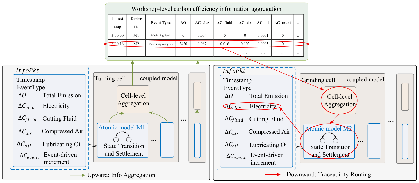
The entire workshop is modeled as a three-layer PDEVS coupled model (equipment, cell, and workshop layers). Based on the formal specification defined in Section 3, the carrier for data flow along the hierarchy is the event information packet, InfoPkt. After each state switch or response to an external event, the equipment atomic model generates an InfoPkt and reports it to the cell aggregation logic to which it belongs via the IC channel. After cell aggregation, it is further summarized into a cell-level carbon efficiency information packet and reported to the workshop aggregation logic. The equipment-level InfoPkt structure is defined as:
InfoPkt   =   ( l ,   type ,   t ,   Δ O , Δ C e l e c , Δ C f l u i d _ u s e , Δ C a i r , Δ C o i l _ u s e , Δ C e v e n t ,   trigger )
where l is the equipment identifier, t y p e is the event type, t is the event occurrence time, Δ O is the physical output increment, Δ C e l e c to Δ C o i l _ u s e are the time-driven carbon emission increments, Δ C e v e n t is the event-driven carbon emission increment, and t r i g g e r is the identifier of the preceding event that triggered this event. This structure unifies the reporting format for all carbon emissions and output increments at the equipment level. It enables each carbon emission change to be traced back to a specific time, event type, and the responsible equipment.
Taking a multi-cell workshop as an example, Figure 2 shows the structure, information channels, and bidirectional data flow of this three-layer PDEVS coupled model.
Within the three-layer coupled model framework, adjacent levels cooperate through two information channels in opposite directions: upward aggregation and downward traceability.
The upward channel supports the real-time monitoring function of carbon efficiency. After each state switch, the equipment atomic model generates an InfoPkt and reports it to the cell aggregation logic via the IC channel. Upon receiving the InfoPkt, the cell aggregation logic immediately accumulates the carbon emissions and output of each equipment, updates the cell-level carbon efficiency, and stores the InfoPkt in the cell event record table with its timestamp. Simultaneously, the cell aggregation logic periodically, or when a significant change in carbon efficiency occurs, reports the aggregated cell carbon efficiency data packet to the workshop aggregation logic. The workshop aggregation logic updates the workshop-level carbon efficiency and stores it in the workshop event record table in the same manner. This mechanism ensures that every change point on the carbon efficiency curve carries a precise timestamp and cause record. Moreover, the information granularity is aggregated stepwise as the level rises. The equipment level retains complete details of each state switch, while the cell and workshop levels maintain only aggregated trends. This avoids redundant uploading of all detailed data.
The downward channel supports the attribution analysis of carbon efficiency anomalies. In practical monitoring, a “significant” decrease is typically defined quantitatively by setting a relative offset threshold (e.g., a 5% drop below the steady-state average) or by employing the 3-sigma rule from Statistical Process Control (SPC) to identify deviations beyond normal operational variance. When the workshop carbon efficiency drops below this predefined threshold within a time interval t 1 t 2 , a traceability query can be initiated. Based on the aggregated data reported by each cell during this interval, the workshop aggregation logic first calculates the approximate decomposition of the workshop carbon efficiency change Δ C E . The contribution of each cell to Δ C E can be calculated as follows:
Δ C E c e l l = ( Δ O c e l l C t o t a l O t o t a l Δ C c e l l ) / ( C t o t a l 2 )
where Δ O c e l l and Δ C c e l l are the physical output increment and carbon emission increment of the cell during this interval, and O t o t a l and C t o t a l are the cumulative amounts of the workshop over the same period. The sum of the contributions of all cells satisfies Δ C E c e l l Δ C E . Cells with a negative contribution (i.e., those exacerbating the carbon efficiency decrease) are identified as responsible cells, locked in descending order of Δ C E c e l l .
After locking the responsible cell, the query is passed to that cell’s aggregation logic. The cell aggregation logic further calculates the contribution of each internal equipment Δ C E l in the same manner:
Δ C E l = ( Δ O l C c e l l O c e l l Δ C l ) / ( C c e l l 2 )
The responsible equipment is locked in descending order of Δ C E l among equipment with a negative contribution. By then extracting the InfoPkt sequence for that equipment within the interval, the specific triggering event can be located. This completes a full three-level traceability from a workshop carbon efficiency anomaly to a cell, equipment, and root cause event.
The above bidirectional mapping mechanism is built upon the event routing of the PDEVS coupled model and the InfoPkt information recording. The workshop-level coupled model is formed by aggregating cell coupled models. Its internal aggregation logic and bidirectional mapping mechanism are completely consistent with those at the cell level, reflecting the structural consistency of the model when extending to multiple cells.

5. Dynamic Carbon Efficiency Monitoring Model for Event Concurrency

Section 4 defined the classification system of carbon emission factors, the carbon efficiency calculation formula, and the multi-resolution information transfer network, which constitute the static network of the model. Based on this, this chapter constructs the dynamic engine to solve two key problems: how carbon efficiency is continuously settled when equipment states change, and how to ensure the uniqueness of the deduction trajectory when multiple events are concurrent.

5.1. State-Driven Dynamic Carbon Efficiency Settlement

The dynamic change of carbon efficiency originates from the equipment’s response to discrete events. To precisely align carbon emission accumulation with state switches, each piece of equipment is modeled as a PDEVS atomic model. A state-factor binding and carbon emission settlement process is built internally. When an equipment state switch occurs due to an event trigger or time advancement, the model automatically settles various carbon emissions and updates the carbon efficiency. This ensures that every change point on the carbon efficiency curve is traceable and interpretable.
Based on the formal atomic model specification in Section 3, we define the domain-specific behaviors for the equipment model M l as follows:
Input Set ( X ): Covers external maintenance and production events, such as failures, repairs, material replenishment, replacements, and parameter adjustments. The output set Y is uniformly fixed as the InfoPkt.
Equipment State ( S ): Described by the tuple m , e , h , where m is the operation mode (taking values from {“Idle”, “Setup”, “Processing”, “Down”, “Starved”}), e is the elapsed time since entering the current mode, and h is the cumulative number of completed qualified workpieces. The distinction between “Idle” and “Starved” (which share identical power states) is to explicitly record the idling cause in the InfoPkt—internal scheduling wait vs. upstream material interruption—thus supporting precise traceability.
Time Advance ( t a s ): When m = “Processing” or “Setup” with a predictable duration, t a s equals the remaining processing or operation time. In other inactive modes, the equipment will not change state autonomously, so t a s = + .
State Transitions ( δ ): Internal transitions ( δ i n t ) correspond to operation completions and are uniformly assigned to priority P2. External transitions ( δ e x t ) handle interventions like failures. When internal and external events collide, confluent transitions ( δ c o n ) are exclusively routed to the rule-driven priority deduction strategy (detailed in Section 5.2) to ensure a deterministic trajectory.
The core of state-driven settlement is state-factor binding: different operation modes activate different carbon emission factors, and settlement is automatically performed when states switch. Table 1 presents the binding relationship between the five modes and time-driven carbon emission factors. Event-driven factors are not bound by mode and are independently triggered by specific events.
The carbon emission settlement upon a state switch follows a unified three-step process, jointly executed by δ i n t , δ e x t , and δ c o n .
Step A: Settle time-driven carbon emission increments. Based on the current mode m and the actual duration Δ t , four increments are calculated. For Δ t : for internal transitions, Δ t = t a ( s ) ; for external or confluent transitions, Δ t = e . State parameters are taken from Table 1 and Appendix A Table A2. The calculation formulas are:
Δ C e l e c = P l , m Δ t E F g r i d
Δ C f l u i d _ u s e = 1 m P r o c e s s i n g f l Δ t E F f l u i d
Δ C a i r = q l , m a i r Δ t S E C c o m p E F g r i d
Δ C o i l _ u s e = r l , m o i l Δ t E F o i l
where 1 m P r o c e s s i n g is an indicator function, taking the value 1 only in the processing state.
First workpiece loading settlement: If the equipment transitions from the Starved or Idle state to Setup or Processing due to material replenishment, and the currently loaded blank has not previously been settled for material carbon, the material carbon emission for this blank should be settled immediately and the N r a w count updated. This settlement is not deferred until processing completion.
Step B: Handle state entry/exit effects. Based on the triggering event type, perform output confirmation, material input, or one-time carbon emission settlement.
Processing completion (internal transition): One qualified piece is confirmed. O l c u m increases by V m a t , l , and h increments by 1. If there are workpieces waiting in the buffer and the tool life limit has not been reached, processing of the next piece begins immediately. If the tool life has been reached, the system transitions to Setup for tool change, and the tool manufacturing carbon emission is accounted for upon tool change completion.
Fault injection and current mode is Processing: The workpiece being processed is scrapped. O l c u m does not increase. The carbon emissions already incurred are not recovered. The state is forcibly transitioned to Down.
Material replenishment completed: The workpiece (blank or work-in-process) enters the equipment buffer. If the equipment is currently in the Starved state and the buffer is non-empty, it automatically transitions to Idle or Setup to prepare for processing. The material carbon emission for a blank is settled immediately when the blank is taken from the buffer and loaded onto the equipment, ready to start its first processing step (i.e., the moment the equipment state officially switches from Starved/Idle to Setup or directly to Processing). This is unrelated to subsequent “processing completion” events. The specific implementation is in the state entry effect of the equipment atomic model.
Tool replacement, cutting fluid replacement, or lubricating oil replacement: The replacement carbon emission is accounted for once according to the formula in Section 4.1. Parameter adjustment: Only subsequent processing time or power parameters are modified, generating no additional carbon emissions.
Step C: Generate output event and update cumulative amounts. All the above increments are encapsulated into an InfoPkt. Time-driven increments are filled in the Δ C e l e c , Δ C f l u i d _ u s e , Δ C a i r , and Δ C o i l _ u s e fields. Event-driven increments are aggregated into the Δ C e v e n t field. Δ O is filled according to the result of Step B: + V m a t , l for one completed piece, 0 otherwise. The t r i g g e r field records the preceding event identifier that triggered this state transition. Finally, the global cumulative amounts are updated:
C l c u m C l c u m + Δ C e l e c + Δ C f l u i d _ u s e + Δ C a i r + Δ C o i l _ u s e + Δ C e v e n t
O l c u m O l c u m + Δ O
Through the above process, every switch in equipment state is accompanied by clear carbon emission settlement and output confirmation. Every change point on the carbon efficiency curve can be accurately traced back to a state transition event, forming an interpretable dynamic trajectory. The complete settlement process during state transitions is detailed in Appendix A Algorithm A1.

5.2. Rule-Driven Concurrent Event Processing

PDEVS collects pending internal and external events at each simulation moment, forming a concurrent event set. If the processing order is uncertain, the carbon efficiency trajectory will be ambiguous. To this end, this section proposes a rule-driven priority deduction strategy for concurrent events. It formalizes manufacturing operation rules into event priorities, suppressing result uncertainty at the mechanism level, so that the carbon efficiency monitoring trajectory is deterministic under the same input.
According to the event’s impact on manufacturing system safety and functional integrity, production recovery conditions, and operational efficiency, events are divided into three priority levels.
P1
Safety and functional integrity disruption. This causes the equipment or system to lose basic functionality and requires an immediate response, typically an unexpected equipment failure. P1 has the highest priority.
P2
Resource and constraint release. This removes obstacles to production recovery or releases equipment capability, including material replenishment completion, fault repair completion, and tool/cutting fluid/lubricating oil replacement. State transition events generated internally by the equipment atomic model (processing completion, tool change completion, etc.) are all assigned to P2. When a preventive maintenance task exceeds its specified window without execution, its priority is automatically upgraded from P3 to P2, reflecting the principle of equipment health priority. Within the PDEVS framework, this expiration is tracked using a dedicated state variable representing the scheduled deadline t scheduled and a Boolean flag indicating completion status maintenance _ done . At any current simulation time t , if the specific condition t t scheduled maintenance _ done = = false is satisfied for a maintenance task, its priority is dynamically upgraded before the Select function evaluates the concurrent event set.
P3
Efficiency adjustment. This optimizes operating parameters when system functionality is intact and there are no production obstacles, typically cutting parameter adjustment. P3 has the lowest priority.
The processing flow is embedded in the event selection logic of PDEVS. The following steps are executed at each simulation moment:
(1)
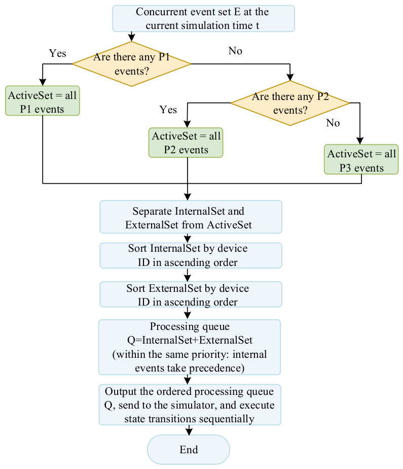
Identify the highest priority category in the current concurrent event set. If P1 events exist, only all P1 events are processed. Otherwise, all P2 events are processed. Only when there are no P1 or P2 events are P3 events processed. Deferred low-priority events are retained until the next simulation moment.
(2)
Within the same priority, internal transition events take precedence over external events to ensure production continuity and state consistency. This rule does not override the higher priority. If an internal event is infeasible in the equipment’s current state (e.g., no processing completion in Starved state), processing is uniformly handled according to Step 3.
(3)
If still indistinguishable, events are processed in a deterministic order, such as ascending order of equipment numbers. It should be noted that sorting by equipment ID is not a mandatory operation; any consistent sorting rule can be applied here. This tie-breaker only dictates the algorithmic execution sequence at the exact same simulation time step t. It does not alter any equipment’s actual state duration, power-time product, output quantity, or material consumption. Therefore, the overall carbon efficiency trajectory remains unaffected, as the accrued emissions and physical output at that specific timestamp are identical regardless of the sorting method.
(4)
The list of concurrent events, the priority determination result, and the actual processing order are written to the audit log to support reproducibility.
Figure 3 visualizes the above logic. Starting from the concurrent event set E , it sequentially checks for the existence of P1 and P2 events to determine the active event set, A c t i v e S e t . If neither exists, all P3 events are processed. A c t i v e S e t is separated into the internal transition event set I n t e r n a l S e t and the external event set E x t e r n a l S e t . After both are sorted in ascending order by equipment number, I n t e r n a l S e t is placed before E x t e r n a l S e t to form the ordered processing queue Q . Deferred low-priority events are rescheduled to the next moment. Each concurrent processing is recorded in the audit log.
This processing strategy directly determines the calling order of the atomic model transition functions. When multiple events arrive at the same equipment simultaneously, the one with the higher priority first triggers δ e x t or δ i n t . The lower-priority one is processed after the current transition is completed and when the state permits. When events act on different equipment, control is exerted through the global event queue order, ensuring a consistent update sequence for multi-equipment states within a cell and a unique carbon efficiency aggregation result.
Under the strict P1 > P2 > P3 priority, when processing completion (internal P2) and fault injection (external P1) occur concurrently for the same equipment, the fault is processed first. The equipment directly transitions to the Down state, and the workpiece being processed is considered an explicit waste product. According to the waste product handling rules in Section 4.1, the completed material removal volume for this workpiece is not counted as effective output, so the carbon emissions numerator does not increase. However, the previously input material embodied carbon and the already incurred processing energy consumption and other carbon emissions have all been fully accounted for in the cumulative carbon emissions, and the denominator is unaffected. Therefore, the instantaneous decrease in carbon efficiency at that moment can still be traced back to the fault event along the InfoPkt. The cause of the anomaly is equally clear and distinguishable, without the need to disrupt the integrity of the global priority system for the sake of output confirmation.
The above three-level priority strategy and the internal event priority rule constitute a complete concurrent processing logic. Table 2 provides general rules for conflict types with examples, eliminating the need to exhaustively list all event combinations. This provides a deterministic processing order for common concurrency scenarios.
This rule system provides an ordered processing basis for various concurrency situations. For example, the aforementioned concurrency of processing completion and fault corresponds to the P1 conflict with P2 rule; the concurrency of tool change and parameter adjustment verified in Section 6.3 corresponds to the P2 conflict with P3 rule. This design effectively suppresses result uncertainty and supports the determinism and reproducibility of the carbon efficiency trajectory. Because these three priority levels are derived from universal manufacturing logic, they are generalizable to other types of workshops, which will be further discussed in Section 6.5. The complete algorithm for concurrent event priority processing is detailed in Appendix A Algorithm A2.

6. Case Study

This chapter takes a machine tool spindle manufacturing workshop as the object and verifies the effectiveness of the model through four progressive scenarios. Section 6.1 establishes a baseline scenario and verifies model accuracy. Section 6.2 introduces a fault event to verify the three-level traceability path. Section 6.3 superimposes concurrent events to verify the determinism of the priority deduction strategy. Section 6.4 examines the robustness of the traceability mechanism through parameter perturbations. Section 6.5 provides a summary and discussion.

6.1. Baseline Scenario and Model Accuracy Verification

The workshop consists of a turning cell and a grinding cell, containing five pieces of equipment. The turning cell includes two lathes, CA6140 and CA6150, which undertake the rough turning process and operate in parallel. The grinding cell includes one cylindrical grinding machine, M1332×1500, and two conical surface grinding machines, C-600CNC and MA1420/500, with the latter two operating in parallel. The workpiece blanks are made of 45 steel (single piece mass 3.0 kg). They undergo rough turning first, followed by cylindrical grinding and conical grinding. A buffer with a capacity of 10 pieces is placed between the two cells, and the normal release interval is 5 min. The parameters used in this case study were collected from the actual manufacturing environment and relevant literature. Specifically, the equipment power data were collected through on-site measurements. The numerical values for the material emission factors were determined in accordance with national and regional carbon emission accounting guidelines applicable to the local manufacturing context, and the accounting logic for the embodied carbon of steel is supported by reference [32]. Other operational parameters, including cutting fluid data, maintenance event parameters, and historical waste rates, were statistically derived from the operational records of the workshop. Carbon emission factors, equipment power and consumption rates, and tool and auxiliary material replacement parameters are detailed in Appendix A Table A1, Table A2 and Table A3.
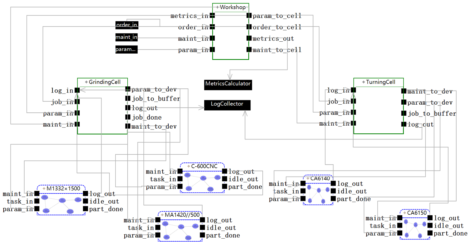
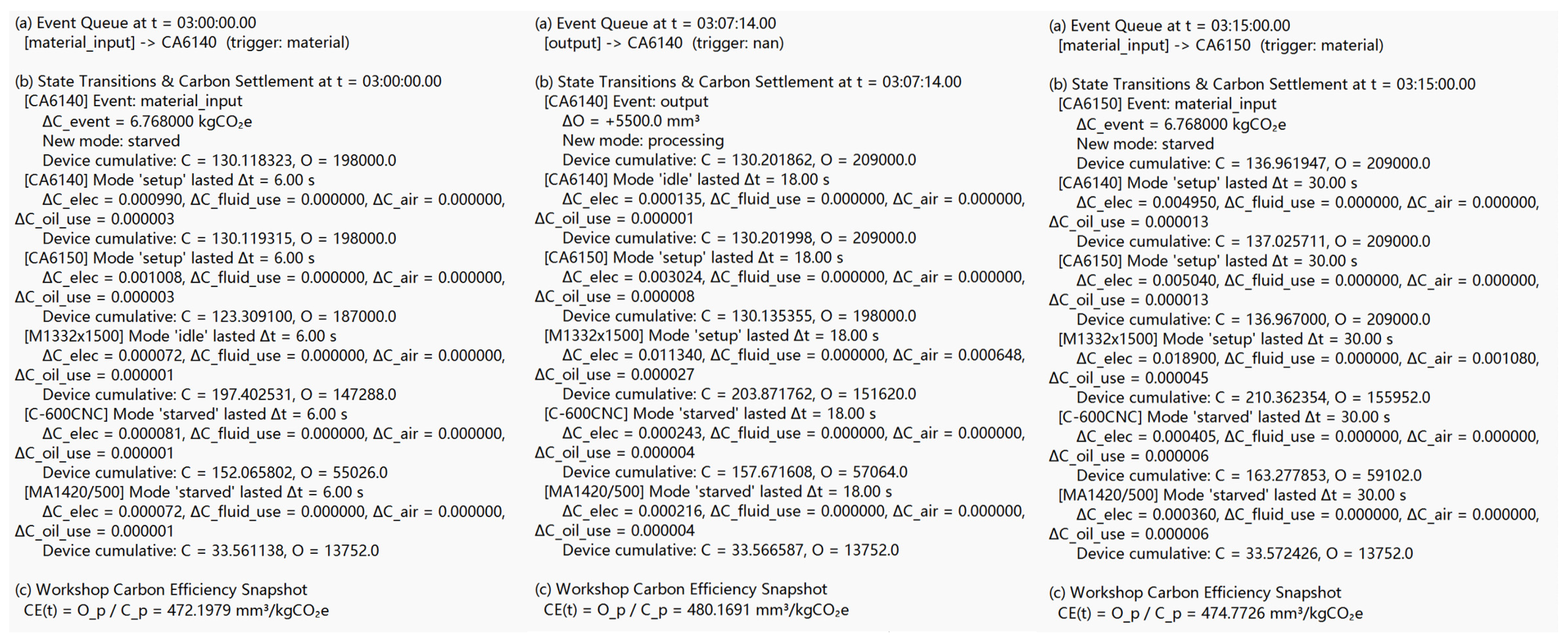
The simulation model is constructed according to the methods in Section 4 and Section 5. Each of the five pieces of equipment is modeled as a PDEVS atomic model, aggregated upward into a cell-level coupled model and a workshop-level coupled model, forming the three-level information transfer network shown in Figure 4. Time-driven emissions are automatically settled with equipment state switches. Event-driven emissions (tool replacement, material input, etc.) are accounted for once when triggered. Waste products are handled according to the rules in Section 4.1. After the simulation ends, the total effective output is corrected by the historical statistical waste rate β = 2 % , while carbon emissions are not deducted. This non-deduction is intentionally designed because the embodied carbon of defective items and the processing energy consumed to produce them have already been physically emitted into the environment. Therefore, these non-value-adding emissions must remain fully accounted for in the overall workshop carbon footprint to accurately reflect the true environmental penalty and the actual carbon efficiency loss caused by waste. Figure 5 captures an output segment from t = 3 :00 to t = 3 :15, showing the complete process of event scheduling, state transitions, carbon emission settlement, and information aggregation, thus verifying the traceability of the deduction process.
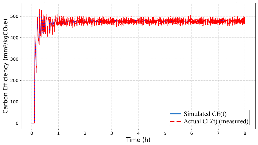
The model was run for 8 h under no-disturbance conditions. A comparison of the workshop carbon efficiency C E ( t ) curve with actual statistical values is shown in Figure 6. Carbon efficiency climbed rapidly from approximately 450 mm 3 kgCO 2 e 1 , entered a steady state after approximately 2.0 h, and fluctuated slightly around 466.73 mm 3 kgCO 2 e 1 , consistent with the trend of the actual workshop statistical curve. The simulated 8 h cumulative carbon emissions were 1728.40 kgCO 2 e , compared to an actual value of approximately 1710.52 kgCO 2 e , yielding a relative error of approximately 1.05%. After correction by the waste rate β = 2 % , the simulated cumulative effective physical output was 823,157 mm 3 , compared to an actual value of approximately 815,920 mm 3 , yielding a relative error of approximately 0.89%. The errors for both indicators were less than 2%, indicating that the model possesses sufficient monitoring accuracy.

6.2. Verification of Traceability Capability Under a Single Fault Event

To verify the three-level traceability path constructed in Section 4.2, a single-fault traceability scenario was set up based on the baseline conditions. After no-disturbance operation until t = 3 :00, the spindle of M1332×1500 in the grinding cell suddenly failed, causing a forced transition from Processing to Down. The downtime for repair was 2 h. Other equipment and material supply remained normal.
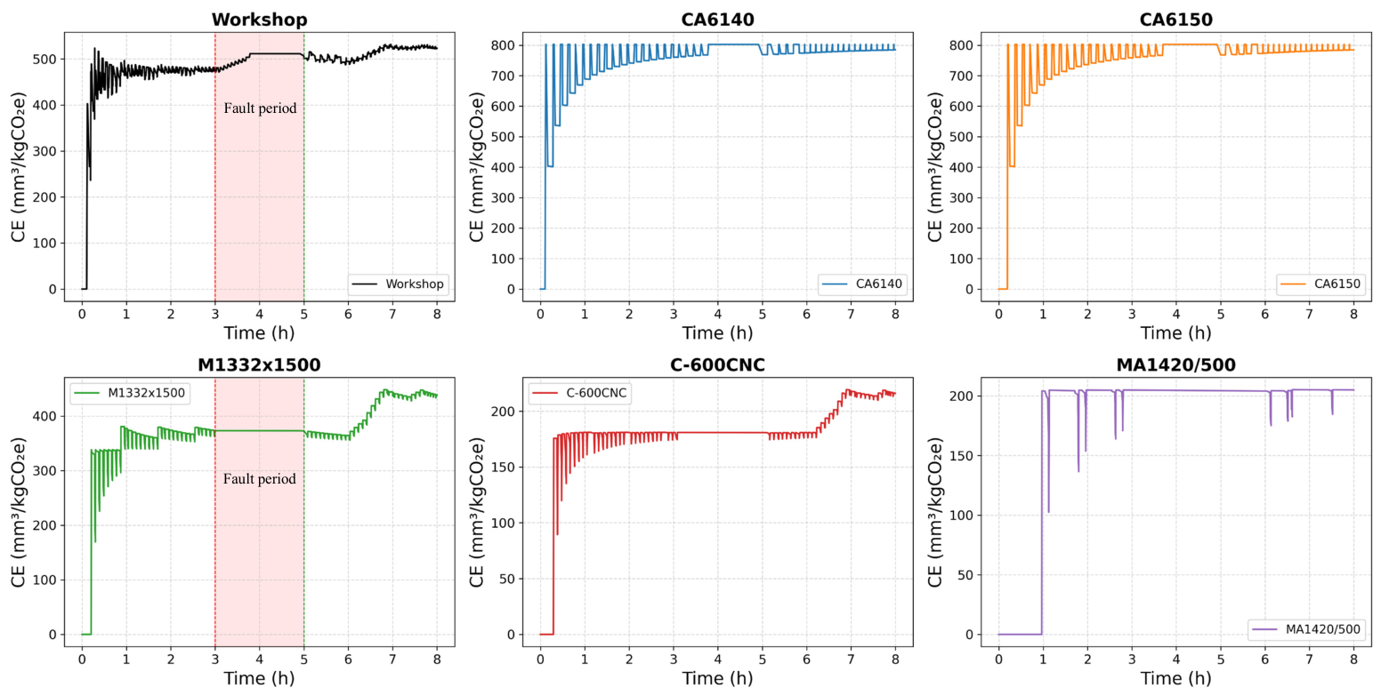
The carbon efficiency curves for the workshop and the five pieces of equipment are shown in Figure 7. The fault period (3:00–5:00) is marked with a red shaded area. The workshop carbon efficiency was stable around 504.86 mm 3 kgCO 2 e 1 before the fault. After the fault was injected, an inflection point appeared at t = 3.00 h, and the efficiency declined continuously, reaching a minimum of 471.60 mm 3 kgCO 2 e 1 at t = 3.08 h, a decrease of approximately 6.6%. After the equipment was repaired at t = 5.00 h, efficiency gradually recovered and returned to the steady-state level at approximately 5.5 h. The differentiated responses of each piece of equipment are evident. The carbon efficiency of M1332×1500 decreased sharply, and its curve decreased monotonically during the fault interval. CA6140 and CA6150 entered Idle due to downstream blockage, and their carbon efficiency clearly declined. C-600CNC assumed part of the transferred tasks, with its carbon efficiency fluctuating slightly. MA1420/500 had no material to process, and its carbon efficiency quickly dropped to zero. Overall, a cascading characteristic of “disturbance–propagation–recovery” is presented.
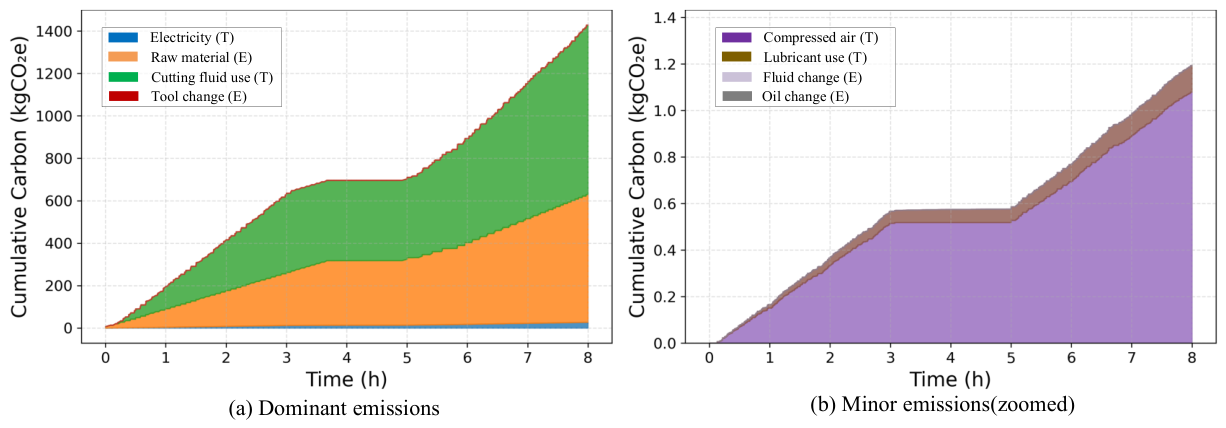
Figure 8 shows the composition of workshop carbon emissions as a stacked chart. The daily consumption of cutting fluid (time-driven) and raw material embodied carbon (event-driven) were dominant. Electricity and tool replacement accounted for relatively small proportions. Among the secondary emission factors, the cumulative trajectories of compressed air and lubricating oil daily consumption are clearly visible. It is worth noting that event-driven emissions from fluid and oil replacements in Figure 8b are zero, as the 8-hour simulation period did not reach their respective replacement thresholds. Over the 8 h period, time-driven emissions accounted for 57.9%, and event-driven emissions accounted for 42.1%.
The changes in carbon emissions and output for each piece of equipment during the fault period are shown in Table 3. M1332×1500 generated only 0.26 kgCO 2 e of idle emissions with zero output. The output increments for the two lathes in the turning cell were both 27,500 mm 3 . Converted by the single-piece material removal volume of 5500 mm 3 , each completed five workpieces. Their carbon emission increments were mainly composed of material embodied carbon and electricity carbon emissions from normal processing. C-600CNC had a carbon emission increase of 5.70 kgCO 2 e and completed 1019 mm 3 of conical grinding output. MA1420/500 had no material to process, with a carbon emission increment of only 0.09 kgCO 2 e .
The carbon emission increments for CA6140 and CA6150 were 41.11 kgCO 2 e and 34.29 kgCO 2 e , respectively, a difference of approximately 6.82 kgCO 2 e , which is close to the embodied carbon of one blank (6.77 kgCO 2 e ). This difference stems from a misalignment in the settlement moment of the blank input. At the beginning of the fault period, CA6140 had just loaded a new blank from the buffer and started processing, simultaneously settling the material carbon for that blank. Meanwhile, CA6150 had not yet loaded a new blank, and its corresponding material carbon had already been settled in a previous processing cycle. Thus, the carbon emission difference between the two is approximately the embodied carbon of one blank. Therefore, this difference is not a double counting error but a result of the coupling between the material carbon settlement timing and the statistical window. After finishing the workpieces in the buffer, both lathes entered the Idle state. The pure idle emissions generated by downstream blockage were minimal, and the carbon emission increments were mainly composed of normal processing activities.
The impact mechanism of the fault on workshop carbon efficiency is as follows. The grinding machine fault caused downstream output to drop to zero. Although the upstream turning cell maintained some processing using buffered work-in-process, the output could only reach the buffer and could not continue downstream. The numerator of carbon efficiency, effective output, was constrained. Simultaneously, the material embodied carbon of the input workpieces and the processing energy consumption were continuously accounted for in carbon emissions, causing the denominator to keep accumulating. The superposition of these two factors led to the continuous decline of workshop carbon efficiency during the fault period. Through the InfoPkt records, the three-level traceability path of “workshop carbon efficiency anomaly → grinding cell → M1332×1500 → spindle fault event” can be traced. The carbon emission and output increments at each level correspond precisely to the triggering event, verifying the traceability of the information transfer network.

6.3. Deterministic Deduction Under Concurrent Events and Multi-Method Comparison

To verify the determinism of the priority processing strategy in Section 5.2, cross-cell concurrent events were superimposed on the single-fault traceability scenario to form a concurrent event deduction scenario. At t = 3 :00, the M1332×1500 spindle fault (P1) occurs. At t = 4 :30, the need for a tool change on CA6140 (P2) and a speed adjustment on C-600CNC (P3) are triggered simultaneously. The tool change takes 3 min and incurs a one-time turning tool manufacturing carbon emission. The speed adjustment only modifies processing parameters, with no additional carbon emissions.
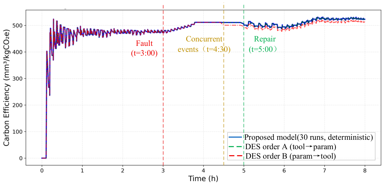
A comparison of the carbon efficiency trajectories between the proposed model and traditional discrete event simulation (DES) is shown in Figure 9. Following the three-level priority strategy (P1 > P2 > P3, with internal events prioritized within the same level), the proposed model consistently processes the P2 tool change before the P3 speed adjustment. The trajectories from 30 runs were identical, and the audit log fully recorded each processing sequence. Traditional DES, lacking a global priority mechanism, determines the execution order of concurrent events based on implementation details. This can produce two different trajectories. Sequence A (tool change first, then speed adjustment) is consistent with the proposed model. Sequence B (speed adjustment first, then tool change) causes additional carbon emission accumulation due to the delayed tool change, leading to a more significant decrease in carbon efficiency. This makes the output results difficult to reproduce.
To quantify the impact of concurrent events on carbon emissions, Table 4 decomposes the carbon emission increment of CA6140, which was directly affected by the tool change event, during the fault period (3:00–5:00). The decomposition clearly separates normal production emissions from tool change event emissions.
As shown in Table 4, the emission increment introduced by the tool change event was only 0.70 kgCO 2 e , accounting for 1.7% of the total increment of CA6140 during the fault period. This portion of emissions originated solely from the tool change operation and was independent of the fault impact. The pure idle emissions during the blockage were only 0.05 kgCO 2 e . The speed adjustment event did not generate additional carbon emissions but maintained the output level during the fault period by improving C-600CNC processing efficiency, playing a positive role in suppressing a further decline in carbon efficiency.
The priority deduction strategy enabled the independent accounting of the impacts of the two concurrent events: tool change and speed adjustment. The carbon emission increment generated by the tool change is clearly distinguishable. The proposed model produced a unique trajectory over 30 runs, with stable impact degrees for each event. This provides a reliable mechanistic guarantee for fine-grained “event–carbon efficiency” attribution, whereas traditional DES cannot achieve this reproducible decomposition due to uncertain execution order.
To further demonstrate the indispensability of the proposed model at the functional level, Table 5 systematically compares this model with several common carbon efficiency monitoring methods used in manufacturing workshops. The comparison dimensions include trajectory determinism, independent decomposition of event impacts, traceability, and adaptability to unseen events.
As can be seen from Table 5, although the statistical analysis method is simple to implement, it lacks event traceability and anomaly response capabilities. Machine learning methods show potential in prediction accuracy, but their inherent black-box nature prevents them from providing an interpretable traceability chain, and the generalization risk for unseen abnormal events is difficult to control. Although traditional DES can simulate dynamic processes, its uncertainty under concurrent events makes it unable to provide a unique carbon efficiency benchmark. Through state-factor binding settlement and priority deduction, the proposed model provides deterministic, traceable, and decomposable carbon efficiency monitoring capabilities with a limited initial modeling cost, making it particularly suitable for scenarios requiring precise operation and maintenance decisions.
Regarding computational complexity, both the proposed model and traditional DES need to maintain a global event queue sorted by timestamp. Assuming the total number of events in the simulation process is N , the complexity of insertion and deletion operations in the event queue is O log N . Therefore, the core complexity of event scheduling for both methods is O N log N . The proposed model additionally introduces a priority sorting step within the concurrent event set: at each simulation time step, if there are M simultaneous events ( M 1 ), they must be sorted according to the three-level priority and internal precedence rules, which has a complexity of O M log M . Since M is the number of concurrent events at the exact same moment, M = 1 in the majority of simulation time steps, and the sorting step is either untriggered or degrades to a trivial operation. The scenario where M 2 occurs only in very rare time steps (e.g., in this case study, M = 2 occurred only once at t = 4 : 30 h), at which point the sorting overhead is far less than the global overhead of event queue maintenance. Therefore, the overall computational complexity of the proposed model is still dominated by O N log N , which is on the same order of magnitude as traditional DES, satisfying the performance requirements for offline analysis and near-real-time monitoring. In terms of implementation difficulty, the proposed model requires additionally maintaining a state-factor binding table and event priority rules; however, this work can be completed once with the equipment templates. Subsequent simulations for different products only require parameter updates, keeping the maintenance cost manageable.

6.4. Verification of Traceability Robustness

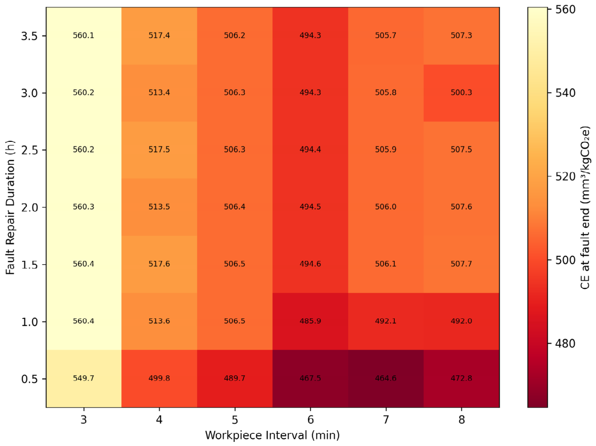
To test the robustness of the traceability mechanism against production parameters, perturbations were applied to the fault repair duration (0.5–3.5 h, step 0.5 h, 7 levels in total) and workpiece release interval (3–8 min, step 1 min, 6 levels in total) based on the concurrent event deduction scenario. This formed a multi-parameter perturbation scenario with 42 parameter combinations. The carbon efficiency at the moment the fault ended and the integrity of the traceability path were recorded.
Figure 10 shows the distribution of carbon efficiency at the fault end moment under each parameter combination using a heatmap. Carbon efficiency was mainly affected by the workpiece release interval. As the interval increased from 3 min to 8 min, the overall C E ( t e n d ) decreased from approximately 560 mm 3 kgCO 2 e 1 to approximately 500 mm 3 kgCO 2 e 1 . This indicates that a tighter production pace corresponds to a higher carbon efficiency at the instantaneous point when the fault ends because more output was accumulated before the fault. The repair duration within the range of 0.5–3.5 h had a relatively small impact on C E ( t e n d ) . Under the same release interval, the difference across different repair durations was less than 15 mm 3 kgCO 2 e 1 . The influence of repair duration is mainly manifested in the subsequent recovery process.
Under all 42 parameter combinations, the traceability path remained complete. The carbon efficiency anomaly could be accurately located to the grinding cell, the M1332×1500 equipment, and the specific fault triggering event. The factor items in the impact degree decomposition had no missing links or chain breaks. This indicates that the traceability mechanism is built upon structural designs such as carbon emission factor classification, the InfoPkt information structure, and the impact degree calculation formula, maintaining its integrity within the tested parameter range.

6.5. Discussion

The case study results reveal two important characteristics of carbon efficiency changes in discrete manufacturing workshops. First, the cascading conduction effect of carbon emissions is significant. Although the fault occurred only on one grinding machine, the negative effect mainly manifested through the blocking of material flow, which stagnated output while carbon emissions from upstream work-in-process continued to accumulate. Second, as revealed in the two-parameter heatmap (Figure 10), both workpiece release intervals and equipment repair durations affect carbon efficiency under fault conditions. However, scheduling-type parameters (such as release intervals) exhibit a significantly greater impact. This is because scheduling directly determines the global production rhythm and the continuous balance between energy consumption and effective output across the entire system. A tighter pacing establishes a higher baseline efficiency that buffers against sudden disruptions, whereas the repair duration primarily dictates a localized, temporary downtime.
A comparison with traditional methods highlights the generalizability and determinism of the proposed model. The state-factor binding mechanism and priority deduction strategy resolve the uncertainty of results under concurrent events, ensuring reproducible trajectories. While the validation is based on a single case study of a spindle manufacturing workshop, the proposed framework provides a standardized modeling approach that can be extended to other discrete manufacturing systems. Core mechanisms—such as the multi-resolution structure, the classification of time/event-driven factors, and the priority rules—are independent of specific product types. Therefore, other manufacturing scenarios, such as automotive components or electronic assembly, can also be modeled using this approach. Similarly, the framework can be applied to analyze various types of production events beyond single machine faults, such as bottleneck shifts, tool wear, or unexpected logistics blockages, as they share the fundamental process of triggering state transitions and generating information packets.
Despite these advantages, the key assumptions of this study and their potential influence on the results must be explicitly summarized. First, the model assumes constant emission factors based on the specific case study. In reality, emission factors vary depending on regional energy mixes, power grids, and supplier conditions. In practical applications across different regions or environments, users must update these emission factor parameters based on localized data. This parameter variation will affect the absolute values of the calculated carbon efficiency, but it does not alter the dynamic event-driven execution mechanism, nor does it affect the accuracy of the transient event-level traceability and impact-degree decomposition. Second, the concurrent event deduction assumes that event priorities and operating rules are predefined and deterministic for a given simulation run. It should be clarified that the three-level priority structure (P1 > P2 > P3) proposed in Section 5 serves as a generalized baseline framework based on typical manufacturing logic. In actual shop-floor practice, this assumption does not restrict operational flexibility. These priority mappings and predefined rules are highly configurable. If human operators dynamically adjust event handling sequences to adapt to complex, real-world emergencies or specific management policies, they can customize and update these priority parameters in the model. The model’s underlying mechanism ensures that regardless of how the rules are customized, the concurrent events will always be executed deterministically according to the newly defined logic, thereby eliminating trajectory ambiguity while maintaining high adaptability to real-world operations.
Finally, regarding applicability and scalability, the current model simplifies the scope by focusing on the machining stage and ignoring assembly and complex logistics. For multi-stage, highly non-linear production lines where cascade effects extend beyond adjacent cells, the proposed multi-resolution PDEVS framework remains structurally scalable. By defining additional coupled models and buffer InfoPkts, the information transfer network can adapt to complex routing. In terms of computational efficiency, the O N log N complexity of the event scheduling ensures that the model can handle standard discrete manufacturing cells efficiently. However, when scaled to highly distributed smart factories with thousands of concurrent events, a single-thread execution may face bottlenecks. Exploring parallel or distributed PDEVS execution engines to enhance computational scalability will be a key direction for future research.

7. Conclusions and Outlook

Aiming at the problems that carbon efficiency fluctuations are difficult to trace and that the impact of each event is difficult to distinguish under multi-event concurrent conditions in discrete manufacturing workshops, this paper proposes a carbon efficiency traceability monitoring model oriented toward event concurrency. This model achieves a dynamic analysis of carbon efficiency with a unique deduction trajectory and traceable fluctuation factors. The main conclusions are as follows:
(1)
A multi-resolution enhanced carbon efficiency information transfer network was constructed, which settles carbon emission factors according to two categories: time-driven and event-driven. By establishing high-resolution atomic models at the equipment level and low-resolution coupled models at the cell/workshop level under the multi-resolution enhanced PDEVS framework, a complete traceability path from workshop-level carbon efficiency fluctuations to specific equipment and carbon emission factors was built. The case study shows that in a single-fault scenario, the traceability path can clearly identify the primary contributing equipment and triggering event, and the impact degrees of each piece of equipment are quantified.
(2)
A dynamic carbon efficiency monitoring model for event concurrency was proposed. It achieves precise alignment of carbon emissions and output through automatic settlement upon state switches, and drives the ordered deduction of concurrent events using a three-level priority rule. This keeps the carbon efficiency monitoring trajectory unique and reproducible. In comparison with traditional DES, the proposed model produced consistent results over 30 runs, and the impact degrees of each event could be independently accounted for, providing a mechanistic guarantee for fine-grained “event–carbon efficiency” attribution.
Taking a machine tool spindle manufacturing workshop as an example, the calculation error of the model for 8 h cumulative carbon emissions under baseline conditions was less than 1.05%, and the steady-state carbon efficiency trend was consistent with actual measurements. In complex scenarios where faults and concurrency were superimposed, the model provided an unambiguous carbon efficiency change curve. It also maintained the integrity of the traceability path under 42 sets of parameter perturbations, demonstrating good robustness.
The above results indicate that the model can provide a transparent and traceable carbon efficiency monitoring method for discrete manufacturing workshops. It helps operation and maintenance personnel identify the causes of carbon efficiency fluctuations under complex event scenarios and provides a quantitative basis for low-carbon operation and maintenance decisions. The adopted PDEVS multi-level coupled framework and priority deduction strategy also offer a reusable modeling paradigm for multi-granularity information fusion and concurrent event processing in manufacturing systems.
Future work focuses on three directions: (1) studying an online adaptive update mechanism for carbon emission factors; (2) feeding traceability results back into priority decision-making for closed-loop control; and (3) improving computational scalability for large-scale, distributed smart factories. To overcome the performance bottleneck of handling thousands of concurrent events, future research will integrate the multi-resolution framework and priority rules with distributed PDEVS execution engines, partitioning coupled models across multiple nodes to decentralize the computational load.

Author Contributions

Methodology, Z.P. and X.C.; Software, X.C.; Formal analysis, X.C.; Investigation, Z.P.; Resources, Z.J.; Writing—original draft, Z.P.; Writing—review and editing, S.Z.; Visualization, Z.P.; Supervision, S.Z., Z.J., and H.Z.; Project administration, S.Z., Z.J. and H.Z.; Funding acquisition, S.Z. and H.Z. All authors have read and agreed to the published version of the manuscript.

Funding

This research was funded by the National Natural Science Foundation of China, grant numbers 52375508 and 51905392.

Institutional Review Board Statement

Not applicable.

Informed Consent Statement

Not applicable.

Data Availability Statement

The data presented in this study are available on request from the corresponding author.

Conflicts of Interest

The authors declare no conflicts of interest.

Appendix A

Algorithm pseudocode for the paper:
Algorithm A1 Carbon settlement on state transition of device atomic model.
Input: current mode m , elapsed time Δ t (h), trigger identifier t r i g g e r , event type e v _ t y p e { fault _ injection ,
material _ input ,   tool _ change ,   fluid _ change ,   oil _ change ,   machining _ complete ,   material _ first _ load } , device parameters P l , m , f l , q l , m air , r l , m oil , M mat , l , V mat , l , V tank , V oil _ tank , emission factors E F grid , E F fluid , S E C comp , E F oil , E F tool , E F fluid _ waste , E F fluid _ new , E F oil _ waste , E F oil _ new , E F mat . In/out: C l cum , O l cum , H l start .
Output:  I n f o P k t , Δ C elec , Δ C fluid _ use , Δ C air , Δ C oil _ use , Δ C event , Δ O .
1: function SettleCarbon ( m , Δ t , t r i g g e r , e v _ t y p e )
2:      // Step A: time-driven carbon settlement
3:       Δ C elec P l , m × Δ t × E F grid
4:      if m = Processing  then
5:          Δ C fluid _ use f l × Δ t × E F fluid
6:      else
7:          Δ C fluid _ use 0
8:      end if
9:       Δ C air q l , m air × Δ t × S E C comp × E F grid
10:        Δ C oil _ use r l , m oil × Δ t × E F oil
11:       // Step B: event-driven settlement
12:        Δ C event 0
13:        Δ O 0
14:       if e v _ t y p e = fault _ injection  and m = Processing  then
15:           Δ O 0  // scrap the part, no output counted
16:       else if e v _ t y p e = material _ input  then
17:          // only update buffer; material carbon deferred to first load
18:       else if e v _ t y p e = tool _ change  then
19:           Δ C event Δ C event + E F tool , l
20:       else if e v _ t y p e = fluid _ change  then
21:           Δ C event Δ C event + ( E F fluid _ waste + E F fluid _ new ) × V tank
22:       else if e v _ t y p e = oil _ change  then
23:           Δ C event Δ C event + ( E F oil _ waste + E F oil _ new ) × V oil _ tank
24:       else if e v _ t y p e = machining _ complete  then
25:           Δ O V mat , l // confirm one qualified output
26:       else if e v _ t y p e = material _ first _ load  then
27:           Δ C event Δ C event + M mat , l × E F mat // account for raw material carbon
28:           H l start H l start + 1
29:       end if
30:       // Step C: accumulate and generate output
31:        C l cum C l cum + Δ C elec + Δ C fluid _ use + Δ C air + Δ C oil _ use + Δ C event
32:        O l cum O l cum + Δ O
33:        I n f o P k t ( l , e v _ t y p e , t , Δ O , Δ C elec , Δ C fluid _ use , Δ C air , Δ C oil _ use , Δ C event ,   t r i g g e r )
34:       return I n f o P k t , Δ C elec , Δ C fluid _ use , Δ C air , Δ C oil _ use , Δ C event , Δ O
35:  end function
Algorithm A2 Concurrent event priority processing.
Input: set of concurrent events E at simulation time t , each event e has attributes (priority { P 1 , P 2 , P 3 } , type { internal , external } , d e v i c e I D ).
Output: ordered processing queue Q ; updated AuditLog.
1: function ResolveConcurrency ( E , t )
2: P 1 { e E e . priority = P 1 }
3: P 2 { e E e . priority = P 2 }
4: P 3 { e E e . priority = P 3 }
5: if  P 1  then
6:    A c t i v e S e t P 1
7: else if  P 2  then
8:    A c t i v e S e t P 2
9: else
10:    A c t i v e S e t P 3
11: end if
12: I n t e r n a l S e t { e A c t i v e S e t e . type = internal }
13: E x t e r n a l S e t { e A c t i v e S e t e . type = external }
14: Sort I n t e r n a l S e t by d e v i c e I D ascending
15: Sort E x t e r n a l S e t by d e v i c e I D ascending
16: Q I n t e r n a l S e t E x t e r n a l S e t // internal events precede external ones of same priority
17: D e l a y e d E A c t i v e S e t
18: Reschedule D e l a y e d to t + ε // defer to next simulation instant, ε is the minimum step size of the simulation clock.
19: a u d i t _ e n t r y ( t , E , A c t i v e S e t , Q , P 1   >   P 2   >   P 3 ;   internal   before   external )
20: Append a u d i t _ e n t r y to A u d i t L o g
21: return  Q
22: end function
Presentation of experimental data related to the paper:
Table A1. Carbon emission factors.
No.Emission SourceSymbolValueUnit
1Grid electricity E F g r i d 0.540 kgCO 2 e / kWh
2Air compressor specific energy S E C c o m p 0.120 kWh / m 3
3Steel raw material E F m a t 2.256 kgCO 2 e / kg
4Cutting fluid production E F f l u i d 2.850 kgCO 2 e / L
5Cutting fluid waste treatment E F f l u i d _ w a s t e 0.710 kgCO 2 e / L
6Cutting fluid new fluid production E F f l u i d _ n e w 2.850 kgCO 2 e / L
7Turning tool manufacturing (per piece) E F t o o l 0.671 kgCO 2 e / piece
8Grinding wheel manufacturing (per piece) E F t o o l 1.625 kgCO 2 e / piece
9Lubricating oil production E F o i l 2.590 kgCO 2 e / L
10Lubricating oil waste treatment E F o i l _ w a s t e 0.650 kgCO 2 e / L
11Lubricating oil new oil production E F o i l _ n e w 2.590 kgCO 2 e / L
Table A2. Equipment operating parameters.
No.ParameterCA6140CA6150M1332×1500C-600CNCMA1420/500Unit
1CellTurningTurningGrindingGrindingGrinding
2Processing typeRough turningRough turningCylindrical grinding/Taper grindingCylindrical grinding/Taper grindingCylindrical grinding/Taper grinding
3Standby power (Idle/Starved)0.050.050.080.090.08kW
4No-load power (Setup)1.101.124.20/4.064.95/4.654.48/4.28kW
5Load power (Processing)2.422.774.85/4.685.60/5.215.20/4.92kW
6Fault power (Down)0.050.050.080.090.08kW
7Preparation time360360250240250s
8Idle running time151310/1413/1610/12s
9Load time (processing time)594865/8057/7060/75s
10Blank mass3.03.0kg
11Material removal mass0.0430.0430.02/0.010.02/0.010.02/0.01kg
12Material removal volume per piece550055002166/12742420/10192420/1146 mm 3
13Compressed air consumption rate (Setup)0.000.002.00/1.801.50/1.301.20/1.00 m 3 / h
14Compressed air consumption rate (Processing)0.000.003.50/3.002.80/2.502.20/2.00 m 3 / h
15Lubricating oil consumption rate (Idle/Starved)0.00010.00010.00030.00030.0003 L / h
16Lubricating oil consumption rate (Setup)0.00060.00060.00210.00250.0025 L / h
17Lubricating oil consumption rate (Processing)0.00200.00200.00690.00830.0083 L / h
18Cutting fluid flow rate0012010090 L / h
Notes: Values before and after “/” correspond to cylindrical grinding and taper grinding, respectively. For M1332×1500, use the first value when performing cylindrical grinding; for C-600CNC and MA1420/500, use the second value when performing taper grinding. Setup duration = preparation time + idle running time; Processing duration = load time. In the Down state, the main drive stops and only the control system maintains basic power; the Down power equals the Idle power, and both compressed air and lubricating oil consumption rates are zero.
Table A3. Auxiliary material and tool replacement parameters.
No.ParameterTurning CellGrinding CellUnit
1Turning tool life200pieces/piece
2Turning tool replacement time3min
3Grinding wheel life300pieces/piece
4Grinding wheel replacement time5min
5Cutting fluid tank volume3000L
6Carbon emission per cutting fluid replacement10,680 kgCO 2 e /replacement
7Hydraulic oil tank volume100200L
8Carbon emission per hydraulic oil replacement324648 kgCO 2 e /replacement
9Statistical waste rate (β)2%2%
Notes: ① Cutting fluid replacement is triggered when the grinding unit reaches 500 operating hours or 10,000 processed workpieces. ② Lubricating oil replacement is triggered when the cumulative operating hours reach 1000 h or the cumulative processed workpieces reach 20,000 (assessed separately for the turning and grinding oil tanks). ③ The priority of all above replacement events is P2.

References

  1. Mencaroni, A.; Leyman, P.; Raa, B.; De Vuyst, S.; Claeys, D. Towards net-zero manufacturing: Carbon-aware scheduling for GHG emissions reduction. J. Clean. Prod. 2025, 529, 146787. [Google Scholar] [CrossRef] [Scilit]
  2. Debbarma, J.; Kumar, V.; Ekundayo, D. Measuring carbon emission efficiency in a developing country: A comparative study of sustainability initiatives and nonsustainability initiatives of manufacturing firms. Bus. Strategy Environ. 2025, 34, 9672–9699. [Google Scholar] [CrossRef] [Scilit]
  3. Diaz C., J.L.; Ocampo-Martinez, C. Energy efficiency in discrete-manufacturing systems: Insights, trends, and control strategies. J. Manuf. Syst. 2019, 52, 131–145. [Google Scholar] [CrossRef] [Scilit]
  4. Yao, M.; Chang, P.; Shao, Z.; Zhang, Q.; Niu, P. Data-Driven Energy Consumption Modeling and Simulation Method of Discrete Manufacturing Workshop Based on Simplified Power Curve. In Proceedings of the 2024 9th International Conference on Automation, Control and Robotics Engineering (CACRE); IEEE: Piscataway, NJ, USA, 2024; pp. 452–459. [Google Scholar] [CrossRef] [Scilit]
  5. Bin, H.; Liu, F.; Zheng, Y.; Yao, Q.; Zhang, Y. Enhancing carbon emission efficiency through the integration of “two industries”: A measurement based on an evaluation index system. Systems 2023, 11, 497. [Google Scholar] [CrossRef] [Scilit]
  6. Hu, S.; Yuan, Z.; Wang, A. Improving carbon emission efficiency in Chinese manufacturing: A study considering technological heterogeneity and noise. Energy 2024, 291, 130392. [Google Scholar] [CrossRef] [Scilit]
  7. Bian, H.; Meng, M. Carbon emission reduction potential and reduction strategy of China’s manufacturing industry. J. Clean. Prod. 2023, 423, 138718. [Google Scholar] [CrossRef] [Scilit]
  8. Zhang, T.; Ji, W.; Qiu, Y. A framework of energy-consumption driven discrete manufacturing system. Sustain. Energy Technol. Assess. 2021, 47, 101336. [Google Scholar] [CrossRef] [Scilit]
  9. Ye, L.; Du, P.; Wang, S. Industrial carbon emission forecasting considering external factors based on linear and machine learning models. J. Clean. Prod. 2024, 434, 140010. [Google Scholar] [CrossRef] [Scilit]
  10. Deng, S.; Zhu, Y.; Tsai, A.; Cooper, D.R. Decarbonizing the US aluminum ecosystem using a dynamic material flow simulation framework. J. Clean. Prod. 2026, 538, 147413. [Google Scholar] [CrossRef] [Scilit]
  11. Li, H.; Cao, H.; Pan, X. A carbon emission analysis model for electronics manufacturing process based on value-stream mapping and sensitivity analysis. Int. J. Comput. Integr. Manuf. 2012, 25, 1102–1110. [Google Scholar] [CrossRef] [Scilit]
  12. Yi, Q.; Li, C.; Tang, Y.; Chen, X. Multi-objective parameter optimization of CNC machining for low carbon manufacturing. J. Clean. Prod. 2015, 95, 256–264. [Google Scholar] [CrossRef] [Scilit]
  13. Zheng, J.; Shi, J.; Lin, F.; Hu, X.; Pan, Q.; Qi, T.; Ren, Y.; Guan, A.; Zhang, Z.; Ling, W. Reducing manufacturing carbon emissions: Optimal low carbon production strategies respect to product structures and batches. Sci. Total Environ. 2023, 858, 159916. [Google Scholar] [CrossRef] [Scilit] [PubMed]
  14. Zhang, C.; Ji, W. Digital twin-driven carbon emission prediction and low-carbon control of intelligent manufacturing job-shop. Procedia CIRP 2019, 83, 624–629. [Google Scholar] [CrossRef] [Scilit]
  15. Zhang, C.; Ji, W. Big Data Analysis Approach for Real-Time Carbon Efficiency Evaluation of Discrete Manufacturing Workshops. IEEE Access 2019, 7, 107730–107743. [Google Scholar] [CrossRef] [Scilit]
  16. Du, Y.; Yi, Q.; Li, C.; Liao, L. Life cycle oriented low-carbon operation models of machinery manufacturing industry. J. Clean. Prod. 2015, 91, 145–157. [Google Scholar] [CrossRef] [Scilit]
  17. Li, H.; Yang, H.; Cao, H.; Zhu, C. State space modelling carbon emission dynamics of machining workshop based on carbon efficiency. Int. J. Comput. Integr. Manuf. 2017, 31, 426–441. [Google Scholar] [CrossRef] [Scilit]
  18. He, B.; Qian, S.; Li, T. Modeling product carbon footprint for manufacturing process. J. Clean. Prod. 2023, 402, 136805. [Google Scholar] [CrossRef] [Scilit]
  19. Sun, Y.; Fu, Z.; Zhao, N. A modular multi-granularity simulation modelling method for manufacturing systems oriented towards digital twins. Int. J. Prod. Res. 2025, 1–12. [Google Scholar] [CrossRef] [Scilit]
  20. Zhang, W.; Zhang, H.; Liu, W. An improved time advance method for distributed multi-resolution modelling with interactive deviation characterization. Simul. Model. Pract. Theory 2024, 134, 102926. [Google Scholar] [CrossRef] [Scilit]
  21. Zhang, L.; Zhuang, C.; Tian, Y.; Yao, M. Construction and Application of Energy Footprint Model for Digital Twin Workshop Oriented to Low-Carbon Operation. Sensors 2024, 24, 3670. [Google Scholar] [CrossRef] [Scilit] [PubMed]
  22. Qian, W.; Guo, Y.; Zhang, H.; Huang, S.; Zhang, L.; Zhou, H.; Fang, W.; Zha, S. Digital twin driven production progress prediction for discrete manufacturing workshop. Robot. Comput.-Integr. Manuf. 2023, 80, 102456. [Google Scholar] [CrossRef] [Scilit]
  23. Li, X.; Cui, G.; Li, S.; Zhang, F. Study of workshop network stability based on pinning control in disturbance environment. Sci. Rep. 2023, 13, 5382. [Google Scholar] [CrossRef] [Scilit] [PubMed]
  24. Fang, W.; Guo, Y.; Liao, W.; Huang, S.; Yang, N.; Liu, J. A Parallel Gated Recurrent Units (P-GRUs) network for the shifting lateness bottleneck prediction in make-to-order production system. Comput. Ind. Eng. 2020, 140, 106246. [Google Scholar] [CrossRef] [Scilit]
  25. Negahban, A.; Smith, J.S. Simulation for manufacturing system design and operation: Literature review and analysis. J. Manuf. Syst. 2014, 33, 241–261. [Google Scholar] [CrossRef] [Scilit]
  26. Wang, X.J.; Choi, S.H. Impacts of carbon emission reduction mechanisms on uncertain make-to-order manufacturing. Int. J. Prod. Res. 2016, 54, 3311–3328. [Google Scholar] [CrossRef] [Scilit]
  27. Cao, H.; Li, H. Simulation-based approach to modeling the carbon emissions dynamic characteristics of manufacturing system considering disturbances. J. Clean. Prod. 2014, 64, 572–580. [Google Scholar] [CrossRef] [Scilit]
  28. Zhou, Y.; Zhou, G.; Zhang, C.; Chang, F.; Wang, Z.; Men, S. Multi-level modeling and robustness evaluation of disturbances in intelligent workshop with temporal snapshot network. J. Manuf. Syst. 2023, 71, 20–33. [Google Scholar] [CrossRef] [Scilit]
  29. Cai, H.; Wan, J.; Chen, B.; Zhang, C.; Zhang, W. Active monitoring of production status in discrete manufacturing workshops driven by digital twins. Int. J. Adv. Manuf. Technol. 2024, 135, 1649–1664. [Google Scholar] [CrossRef] [Scilit]
  30. Zeigler, B.P. Using the parallel DEVS protocol for general robust simulation with near optimal performance. Comput. Sci. Eng. 2017, 19, 68–77. [Google Scholar] [CrossRef] [Scilit]
  31. Batchoudi, G.; Ramat, E.; Foucher, C. FPDEVSML: A platform-independent parallel-DEVS specification language. SIMULATION 2026. [Google Scholar] [CrossRef] [Scilit]
  32. Fang, X.; Sun, W.; Li, W.; Ma, G.; Wang, P.; Zuo, C. Process-based life cycle inventory framework for assessing the carbon footprint of products from complex production paths: Case of dual-phase automotive strip steel. J. Clean. Prod. 2024, 447, 141551. [Google Scholar] [CrossRef] [Scilit]
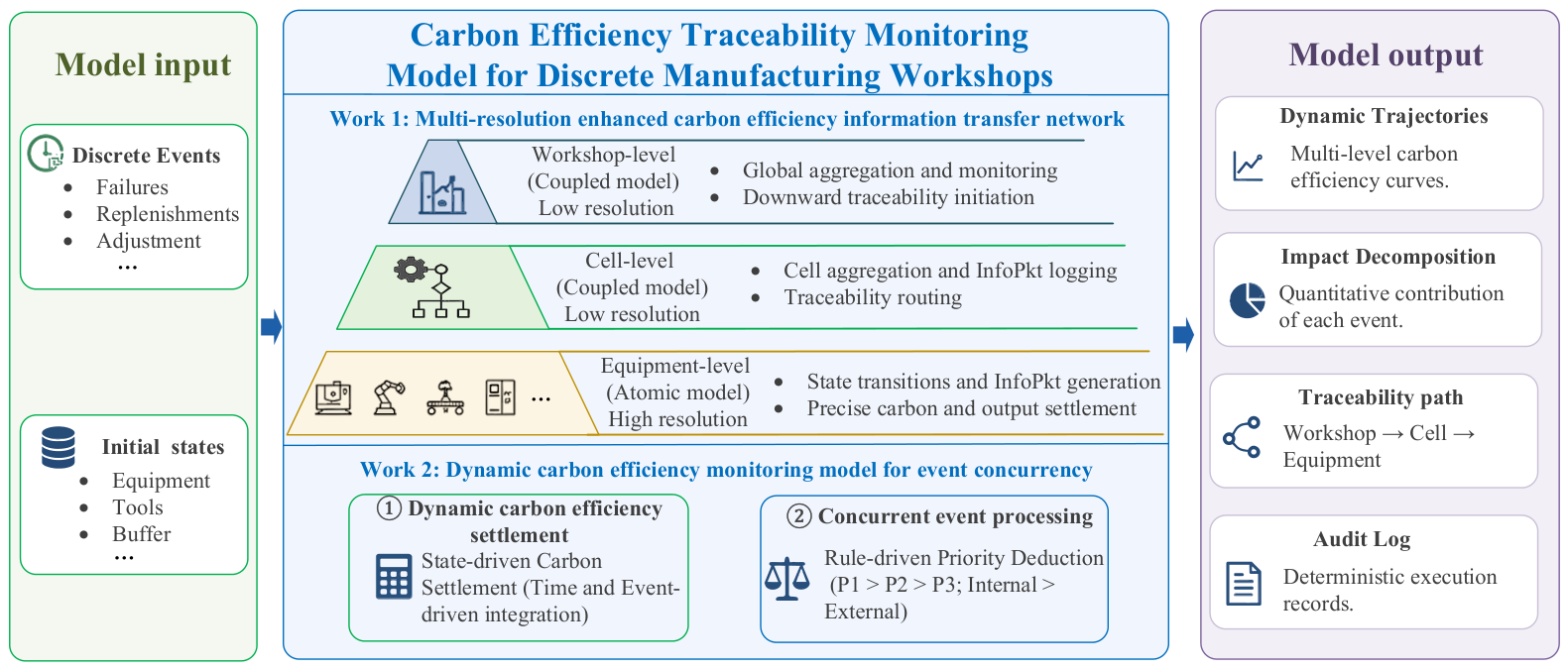
Figure 1. Methodological framework.
Sustainability 18 08363 g001
Figure 2. Structure of the carbon efficiency information transfer network.
Sustainability 18 08363 g002
Figure 3. Deterministic processing flow of concurrent events.
Sustainability 18 08363 g003
Figure 4. Workshop entity modeling.
Sustainability 18 08363 g004
Figure 5. Example of carbon efficiency output.
Sustainability 18 08363 g005
Figure 6. Model accuracy comparison.
Sustainability 18 08363 g006
Figure 7. Workshop carbon efficiency curves under M1332 fault.
Sustainability 18 08363 g007
Figure 8. Workshop carbon emission traceability.
Sustainability 18 08363 g008
Figure 9. Model comparison under concurrent events.
Sustainability 18 08363 g009
Figure 10. Two-parameter heatmap.
Sustainability 18 08363 g010
Table 1. Binding of equipment states and time-driven carbon emission factors.
StateElectricity Carbon EmissionsCutting Fluid Consumption Carbon EmissionsCompressed Air Carbon EmissionsLubricating Oil Consumption Carbon EmissionsAttribution
IdleStandby powerNoneNoneTrace (intermittent supply)Scheduling waiting within this cell
SetupPreparation powerNoneYes (tool change/fixturing)Yes (tool holder/guideway movement)Process preparation for this equipment
ProcessingProcessing powerYes (by flow rate)Yes (chip blowing/fixture holding pressure/air sealing)Yes (full load lubrication)Normal production activity
DownFault powerNoneNoneNoneThis equipment fault
StarvedStandby powerNoneNoneTrace (intermittent supply)Upstream material supply
Table 2. Concurrent event priority processing rules.
Conflict TypeProcessing Rule
P1 conflict with P2/P3P1 takes the highest priority; P2/P3 are deferred. Safety and functional integrity events cannot be interrupted. Example: If a sudden failure (P1) occurs during a tool change (P2) or parameter adjustment (P3), the current operation is immediately interrupted to prioritize fault handling.
P2 conflict with P3P2 takes priority over P3. Removing obstacles to production recovery takes precedence over efficiency optimization. Example: If the equipment simultaneously receives a parameter adjustment (P3) instruction and a material replenishment completion (P2) signal, material replenishment is executed first. When preventive maintenance is overdue, it is automatically upgraded from P3 to P2, reflecting the principle of equipment health priority.
Conflict within the same priorityInternal state transition events take precedence over external injection events to ensure production continuity and state consistency. Example: If equipment processing completion (internal P2) and a tool replacement instruction (external P2) are triggered simultaneously, the current processing output and carbon emissions are settled first, then the tool change is executed.
Conflict still remains after the above rulesProcessed in a deterministic order (e.g., ascending order of equipment numbers). This sorting method is not mandatory and only ensures trajectory reproducibility at the exact same time step. It does not alter any equipment’s state duration, energy consumption, or physical output, thus leaving the total carbon efficiency unaffected. Example: If two different pieces of equipment fail simultaneously (P1), they are processed in numerical order.
Table 3. Changes in equipment carbon emissions and output during the fault period (3:00–5:00).
EquipmentCarbon Emission Increment ( kgCO 2 e )Increment Proportion (%)Output Increment ( mm 3 )Status Description
M1332×15000.260.30Downtime due to fault; only basic power maintained
C-600CNC5.707.01019Undertook transferred tasks; load slightly increased
MA1420/5000.090.10No material to process; entered Starved
CA614041.1150.527,500Processed five pieces; mainly material carbon and electricity consumption; entered Idle after processing due to downstream blockage
CA615034.2942.127,500Processed five pieces; mainly material carbon and electricity consumption; entered Idle after processing due to downstream blockage
Total81.4510056,019
Table 4. Decomposition of CA6140 carbon emission increment during the fault period.
Emission SourceEmission Amount ( kgCO 2 e )Proportion of CA6140 Increment (%)Description
Subtotal of normal processing emissions41.1198.3Includes material embodied carbon of five processed workpieces, electricity, lubricating oil consumption, trace idle emissions during blockage, and material carbon settlement for previous workpieces
Tool change event emissions0.701.7Includes turning tool manufacturing carbon emission and electricity consumption in Setup state during the tool change
Total41.81100
Table 5. Characteristic comparison of different carbon efficiency monitoring methods.
CharacteristicProposed Model (PDEVS + Priority)Traditional DESStatistical AnalysisMachine Learning
Trajectory determinismCompletely deterministic; identical results across 30 runsUncertain; depends on internal event sequenceOnly provides smooth trends; cannot reflect transient fluctuationsProbabilistic output; inherent uncertainty
Independent decomposition of event impactsCan independently quantify carbon emission increments caused by each event (e.g., tool change event 0.70 kgCO2e)Cannot be independently decomposed; event impacts are aliasedCannot be decomposed to the event levelBlack-box model; cannot provide factor decomposition
TraceabilityThree-level traceability; can be located to equipment, states, and specific factorsPartially traceable to equipment; event causes are ambiguousLacks event-level traceabilityLacks event-level traceability
Adaptability to unseen eventsMechanism-based state-driven; requires no historical fault dataSame as the proposed model; relies on mechanism modelingCannot handle abnormal events not present in historical dataGeneralization depends on training set coverage; prone to large errors for unseen events
Implementation difficultyRequires predefined state-factor binding, priority rules, and InfoPkt structure; slightly higher initial modeling effortModerate; requires constructing state charts and event listsLow; based on average emission factor accountingHigh; requires massive annotated data and model tuning
Disclaimer/Publisher’s Note: The statements, opinions and data contained in all publications are solely those of the individual author(s) and contributor(s) and not of MDPI and/or the editor(s). MDPI and/or the editor(s) disclaim responsibility for any injury to people or property resulting from any ideas, methods, instructions or products referred to in the content.