A Study on the Optimization of Site Selection and Capacity Allocation for New Energy Vehicle Swapping Stations in Urban Areas

Abstract

Urban battery swapping station (BSS) planning is difficult because site opening, service-module allocation, user assignment, battery degradation pressure, travel burden, and congestion are tightly coupled. A plan that minimizes investment alone may create long queues, whereas a plan that only reduces waiting can overbuild costly and underused capacity. This study formulates the urban BSS siting–sizing problem as an operation-aware mixed-integer nonlinear model and evaluates feasible plans with payoff-table global-criterion normalization. To search this rugged planning space, we propose a Stable Portfolio Hyper-Heuristic (SPHH) that combines Greedy construction, BO-guided large-neighborhood search, simulated annealing, and optimized annealing with reheating, followed by feasible-incumbent preservation and non-worsening post-processing. The formal campaign contains 18 synthetic cases, 10 independent repeats, and five algorithms, yielding 900 optimization records. Across the 18 cases, SPHH produced the lowest mean GC score and reduced the mean GC value on average relative to the baseline algorithms. Nonparametric Friedman and Holm-adjusted Wilcoxon tests confirmed statistically significant differences among methods, although the advantage over the strongest baseline was not universal. These results indicate that SPHH is most useful as an offline planning selector that improves recommendation stability when additional computation is acceptable, rather than as a universally faster optimizer.

1. Introduction

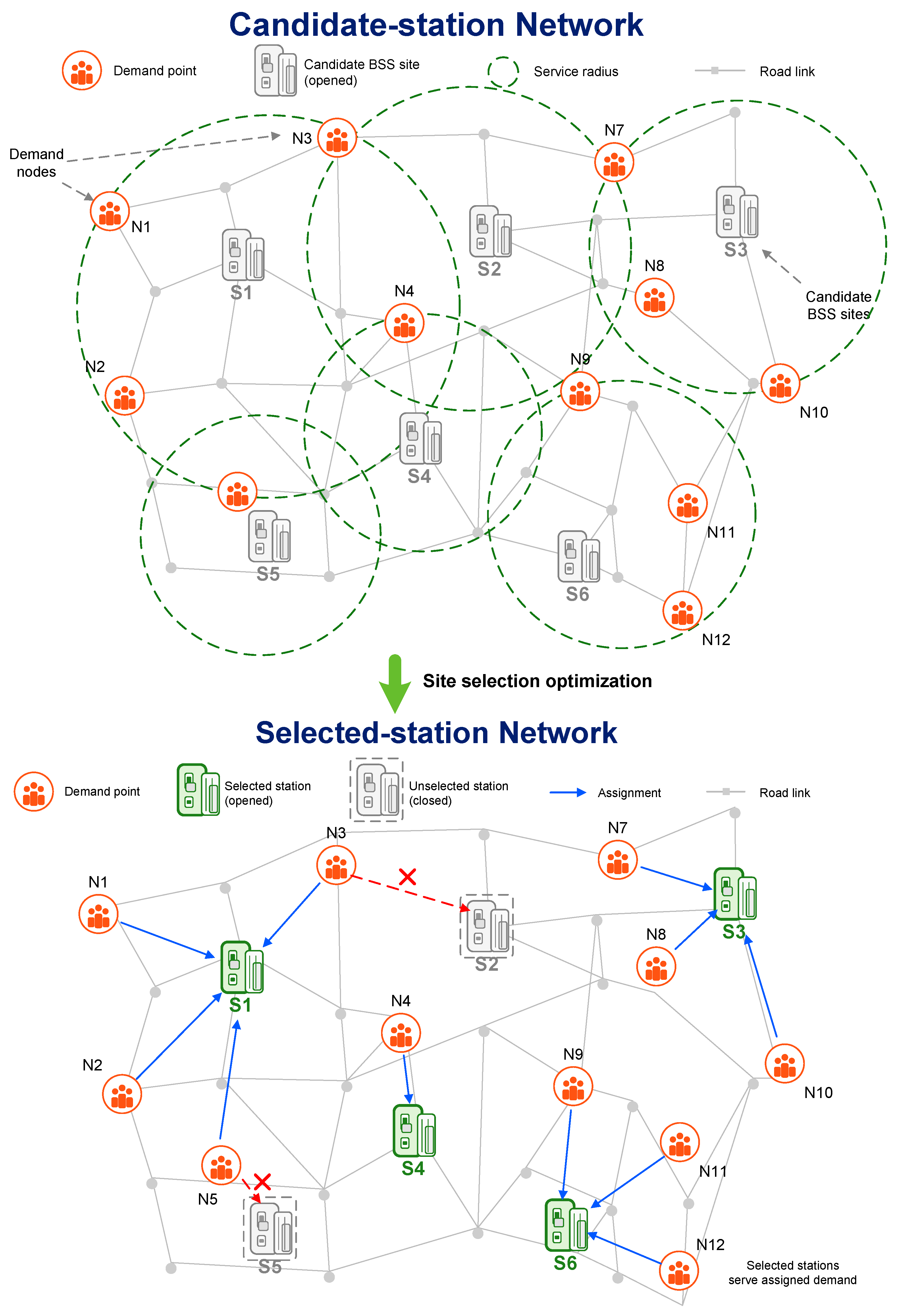
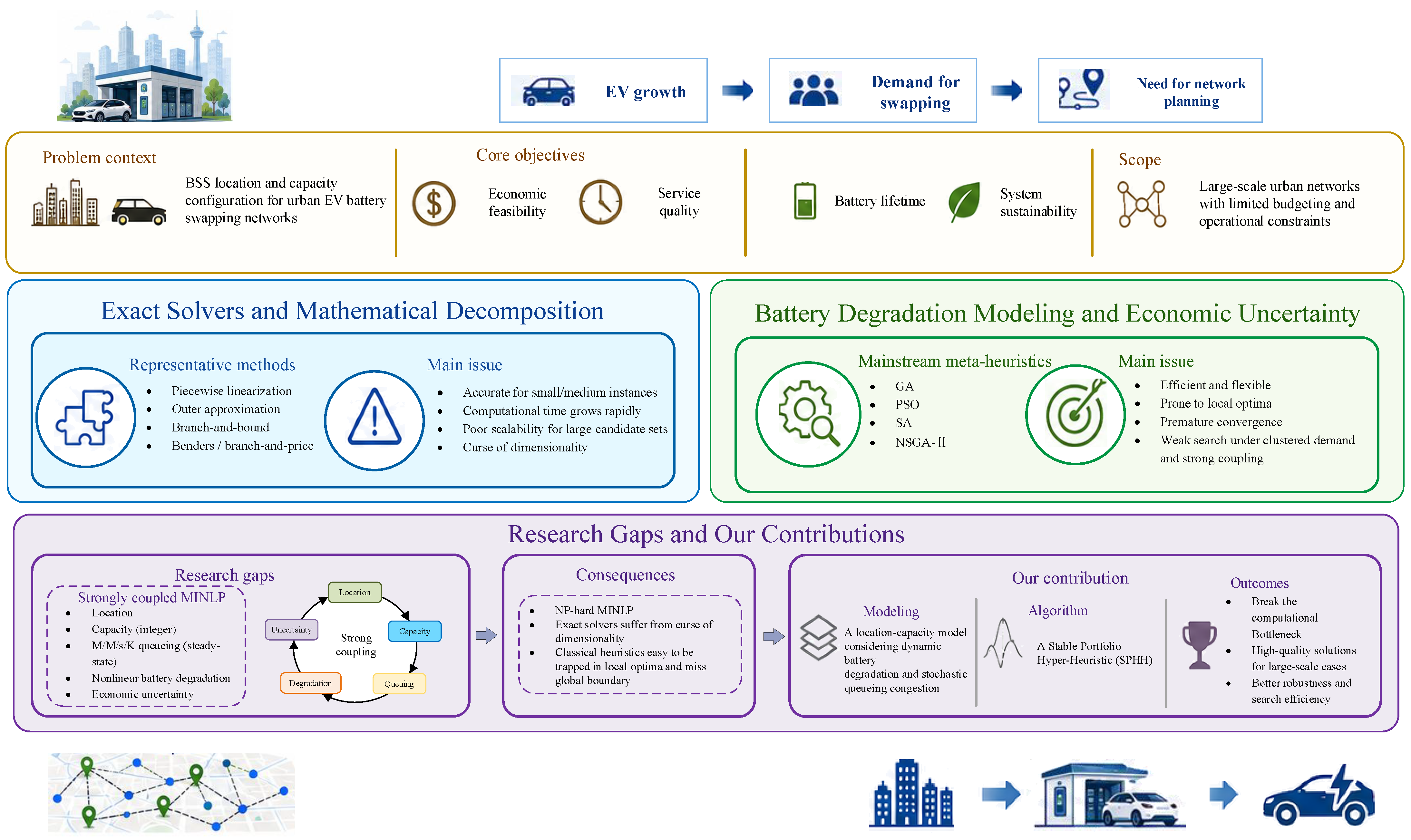
The rapid growth of electric vehicles (EVs) has changed urban energy-replenishment planning from a problem of simply adding charging points into a problem of designing a reliable service network [1,2,3]. Plug-in charging can satisfy many private-vehicle scenarios, but it is less suitable for taxis, logistics fleets, buses, and heavy-duty vehicles that operate under tight schedules and cannot tolerate long and uncertain downtime. Battery swapping stations (BSSs) provide a different operating logic: the vehicle-side service is a short battery exchange, while the operator absorbs charging, battery circulation, spare-battery inventory, and equipment scheduling. This separation can improve fleet availability and reduce user dwell time, but it also makes infrastructure planning more consequential. A station is not only a geographical facility; it is a coupled operating unit whose location and capacity decisions affect user access, congestion, battery use intensity, and life-cycle cost. For this reason, urban BSS deployment should be formulated as an operation-aware site selection and capacity allocation problem rather than as a conventional facility-location task. The overall research framework of this study is summarized in Figure 1.

The necessity and significance of this study arise from the high investment cost, long service life, and limited reversibility of BSS infrastructure decisions. Once a station is built and its service capacity is installed, the operator cannot easily relocate land resources, modules, chargers, and battery inventories in response to later demand changes. The operating burden transferred from users to the station operator also means that a BSS plan must account for more than distance reduction. Location-routing studies show that station opening and user assignment jointly shape investment and service outcomes [4,5]. In dense urban areas, BSS siting also depends on spatial demand, road accessibility, and multiple suitability criteria [6,7,8,9]. A site close to a demand cluster can reduce user travel cost, but if the assigned service modules are insufficient, the station becomes congested and the advantage of proximity is lost. Conversely, deploying high capacity across many candidate sites can reduce queues, but it may create idle equipment, underused batteries, and excessive land and construction investment. Battery value, state-of-health evolution, charging strategy, and replacement timing further affect the long-term return of BSS investment [10,11]. The central research pain point is therefore not whether location and capacity are both important, but how to decide them simultaneously when every decision changes the economic meaning of the others. Opening one station reshapes the feasible assignment set of nearby demand points. Increasing the number of service modules changes the service rate, utilization, queue length, waiting probability, battery circulation intensity, and degradation pressure. Reassigning users changes station loads and may turn a previously reasonable capacity plan into an overloaded or idle configuration.

This study combines finite-capacity queueing, battery-life estimation, stochastic cost modeling, degradation, and data-driven siting mechanisms that have been examined separately in related infrastructure studies [12,13,14,15,16]. Their integration produces a mixed-integer nonlinear model with discrete thresholds and many local trade-offs. Here, M/M/s/K follows Kendall’s notation: the first M denotes Poisson vehicle arrivals, the second denotes exponentially distributed service times, s is the number of parallel service channels, and K is the maximum number of vehicles in the system, including those in service and waiting. Each battery-swapping module is treated as one service channel, so $s_j=m_j$. In practical terms, the queueing component is not a smooth cost that declines linearly with each added module. Waiting time can drop sharply when a station crosses a service-capacity threshold, while degradation and replacement costs may increase as utilization and battery cycling become more intensive. This opposing movement between congestion relief and life-cycle cost creates a rugged objective surface in which small changes in capacity or assignment can cause large changes in total cost. The difficulty is therefore not only computational scale; it is also the risk of obtaining a plan that looks feasible under simplified assumptions but performs poorly in operation. If queueing is ignored, nearby users may be assigned to stations that cannot serve them within an acceptable waiting time. If degradation is ignored, high-utilization stations may appear economically attractive while hidden replacement costs accumulate. If travel cost and construction cost are optimized without service reliability, the network may either overbuild expensive capacity or shift inconvenience to users. These consequences show why BSS planning requires an integrated model rather than separate decisions for siting, sizing, assignment, and operation. They also create a practical dilemma: a model detailed enough to represent operation may be difficult to solve repeatedly across many candidate sites, demand points, and scenario settings, while a simpler search method may produce unstable recommendations when demand clusters, capacity thresholds, or road accessibility change.

Related studies on flexible infrastructure show that operational coordination must account for uncertainty and cross-network dependence. Qin et al. coordinated data-center workloads and building thermal flexibility as a virtual storage system through two-stage distributionally robust optimization [17]. Li et al. coordinated building thermal flexibility and E-Bus mobility for post-disaster restoration in coupled power and transportation networks [18]. These studies demonstrate the value of flexible resources, but their decision settings begin after infrastructure locations and capacities have been determined. They therefore do not address the irreversible pre-deployment choices central to BSS planning, including station opening, module allocation, and demand assignment.

Prior studies have established important building blocks, but one planning question remains unresolved: how can an urban BSS network be sited and sized when station opening, integer service modules, user assignment, queueing thresholds, and battery life-cycle cost change one another rather than acting as separable inputs? Exact and decomposition models define rigorous location-routing structures [19,20], but extending those structures while retaining all operational feedbacks at urban scale remains difficult. Meta-heuristics search nonlinear and discrete spaces more flexibly [21,22], although their recommendations can vary with encoding, initialization, neighborhood design, and parameter choices. This paper therefore develops an operation-aware siting-sizing framework that keeps the cost logic transparent while using a Stable Portfolio Hyper-Heuristic (SPHH) to search across feasible network configurations. The contribution is to turn BSS deployment from a static facility-location task into a joint investment-service decision in which site opening, module allocation, demand assignment, waiting reliability, and battery-related expenditure are evaluated within one planning objective.

2. Literature Review

2.1. Queueing, Degradation, and Economic Uncertainty in BSS Planning

Recent BSS studies increasingly recognize that station capacity is an operating decision rather than a static attribute attached to a selected site. Multi-objective planning and simulation studies have incorporated construction expenditure, service performance, and battery degradation to describe station economics more realistically [12,23,24]. Battery valuation, state-of-health, and degradation-dependent economic studies show that batteries and service modules create costs through acquisition, depreciation, cycling, and replacement timing [10,13,15,25,26]. Demand-flow, user-choice, queueing, and dispatch studies add a user-side layer through access distance, waiting delay, service availability, and demand uncertainty [16,27,28,29,30]. Stochastic cost modeling in related energy infrastructure also shows that long-term evaluation can change when uncertain cost streams are represented explicitly [14].

For the siting-sizing model developed in this paper, the key lesson from this stream is that module value depends on station load: the same module can substantially reduce waiting at a congested site, but it can also become an idle asset at a weak-demand site. A recent congestion-oriented study by Zhang, Li, and Saldanha-da-Gama explicitly incorporated waiting-time constraints into the location of single-server BSSs, which makes the service-reliability issue more visible [31]. However, the single-server and maximal-covering setting does not represent multi-module capacity allocation, battery circulation, or degradation-related cost within the same planning objective. For urban BSS deployment, the remaining difficulty is that queueing, degradation, and economic mechanisms are often optimized in partial combinations. Queueing-aware models can reduce waiting time but may treat battery degradation or replacement cost as secondary. Degradation-aware studies can capture battery health more carefully but may simplify spatial assignment and service congestion. Economic models can describe discounting and replacement expenditure but may be too aggregate to guide site-level capacity allocation. Operation-management studies can improve dispatching or charging schedules after stations exist, but they do not always answer where stations should be opened and how much capacity should be installed before operation begins [11,30]. This fragmentation has direct planning consequences. A plan that minimizes waiting alone may overbuild modules and leave expensive equipment underused outside peak periods. A plan that minimizes battery wear alone may send users to distant or congested stations, shifting cost from the operator to travelers. A plan that minimizes construction cost alone may appear inexpensive but fail under peak demand, creating long queues and reducing fleet availability. These outcomes are not separate errors; they are forms of cost transfer within the same system. The literature therefore points toward an integrated approach in which waiting delay, degradation pressure, and investment cost are evaluated together.

2.2. Robust Coordination and Resilience in Coupled Flexible Infrastructure

Research on coordinated flexible infrastructure provides complementary operational context for BSS planning. Qin et al. modeled data-center buildings and adjustable cloud workloads as a virtual storage system [17]. Their framework represents building thermal dynamics and differentiated computing demands under uncertainties in general loads and outdoor temperatures. An imprecise Dirichlet model constructs data-driven uncertainty sets, and a two-stage distributionally robust formulation adjusts the conservativeness of the operating strategy. A Dynamic Accuracy Column and Constraint Generation algorithm solves the resulting problem. The study shows how flexible demand and thermal inertia can improve operating economy, computing efficiency, and resilience under uncertainty.

Li et al. examined cross-infrastructure coordination in coupled power and transportation networks [18]. Their post-disaster restoration model integrates building thermal dynamics with E-Bus path planning. It uses air-conditioning flexibility and the spatio-temporal mobility of E-Buses to extend critical-load supply while limiting travel distance. A double-judgment asynchronous decentralized alternating direction method of multipliers algorithm supports parallel solution while protecting information held by different network operators. The study therefore focuses on emergency restoration, decentralized coordination, and network resilience after disruptive events.

These studies and the present work share the principle that infrastructure value depends on coordinated operational flexibility. However, their decision stages, uncertainty treatments, and planning objectives differ. Qin et al. optimize short-term data-center operation under distributional uncertainty, whereas Li et al. optimize post-disaster restoration of an existing electricity-transportation network. The present study instead addresses strategic BSS deployment before operation by jointly determining station opening, integer service modules, demand assignment, queueing delay, and degradation-related expenditure. It does not model distributional ambiguity or emergency restoration. Here, stability refers to reliable feasible-solution search across discrete planning instances and repeated runs, rather than to distributional robustness or post-disaster network resilience. These distinctions establish the scope of the planning model and motivate a reliable search strategy for heterogeneous BSS instances.

2.3. Classical Meta-Heuristics for Infrastructure Planning

Classical meta-heuristics are widely used in EV infrastructure planning because the decision space is discrete, nonlinear, and difficult to solve under strong convexity assumptions [32,33]. Improved genetic algorithms have been applied to charging and battery-swap station location problems, and related scheduling or allocation studies have used heuristic or cascaded optimization to coordinate vehicle routing, charging decisions, station operation, and service assignment [11,21,22,34,35]. Adaptive swarm and grey-wolf variants have also been proposed to improve exploration and convergence in BSS optimization [36,37]. These methods are valuable because a feasible BSS plan must encode station openings, capacity levels, and demand assignment while satisfying service and cost constraints that are hard to linearize. However, their limitation is not only approximation error but also sensitivity across planning instances. A genetic algorithm can be affected by chromosome encoding, crossover design, mutation probability, and penalty treatment. Swarm-based algorithms may lose interpretability when binary site variables and integer module numbers dominate the decision vector. Simulated annealing can escape local optima, but its effectiveness depends on the neighborhood structure, acceptance rule, and cooling schedule. These sensitivities matter because urban BSS instances differ in demand clustering, candidate-site density, road accessibility, and capacity thresholds. A method that performs well in one spatial pattern may converge prematurely or recommend a different investment level under a slightly changed demand distribution. The consequence is practical rather than merely computational: station opening and module-sizing recommendations may change with encoding choices, random seeds, or penalty settings, making it difficult for planners to judge whether a capacity plan is robust enough for long-lived infrastructure investment. Existing meta-heuristic studies therefore motivate flexible search approaches that can work across different demand and capacity scenarios.

2.4. Exact Optimization and Mathematical Decomposition

Exact optimization remains important because it makes the structure of the planning problem explicit and provides a benchmark for interpreting heuristic results. Facility-location models, Benders decomposition, branch-and-price methods, and bi-level formulations have clarified how station placement, vehicle routing, service decisions, and cost allocation interact in EV charging and swapping systems [5,19,20]. Chen et al. used a branch-and-price framework with adaptive selection for a mixed-fleet battery swap station location-routing problem with time-window constraints, which provides a strong exact-and-heuristic benchmark for routing-location interaction [20]. Zhang et al. developed a bi-level model for union BSS location-routing under joint distribution and cost allocation, showing how collaborative distribution and cost sharing can be represented in a structured planning model [5]. Recent reviews and two-layer planning studies also show that hierarchical and exact formulations are useful for separating strategic investment decisions from tactical or operational service decisions [32,38,39]. This rigor is valuable for BSS planning because exact models can define feasibility, reveal binding constraints, and expose trade-offs between investment and service quality before a heuristic search is introduced.

The exact-modeling literature becomes most limited at the point where the model must reproduce daily BSS operating behavior. The exact and decomposition studies above clarify routing, cost allocation, and feasibility, but they do not fully endogenize service-module capacity, queueing delay, user assignment, and battery degradation within one life-cycle siting objective. Module numbers affect service rate, utilization, waiting time, battery cycling, and degradation pressure at the same time [24,26,31,40,41]. Opening a station changes assignment feasibility, while reallocating demand changes the load and waiting cost at multiple stations. User choice, traffic-network demand estimation, and stochastic arrivals further weaken the separability that many decomposition methods rely on [27,28]. In a simplified formulation, station opening, demand assignment, and capacity deployment can often be separated into cleaner subproblems. In an operation-aware formulation, however, these decisions repeatedly feed back into each other. A small capacity increase may reduce queueing cost sharply at one station, but the same change may also raise battery use intensity and replacement pressure. A small reassignment may relieve one station while making another station congested. These threshold effects and feedback loops make the planning problem harder to decompose without losing the operational meaning of the solution. This limitation has practical consequences. If exact formulations simplify queueing to preserve tractability, the selected network may be mathematically optimal but unable to absorb peak arrivals, leading to long queues and poor service reliability. If battery degradation and replacement costs are omitted, high-utilization stations may look cost-effective in the model while creating hidden life-cycle expenditure after deployment. If assignment and traffic-network demand are simplified, the model may recommend sites that reduce construction cost but increase user detours, uneven station loads, and waiting time. These trade-offs show why exact methods alone may not be sufficient for operation-aware BSS planning, and why heuristic approaches need to incorporate operational mechanisms explicitly.

2.5. Hybrid and Hyper-Heuristic Search

Hybrid and hyper-heuristic methods are useful when no single search logic is consistently best across all instances. Reviews of EV infrastructure and energy-replenishment optimization report a broad range of constructive, exact, and meta-heuristic algorithms [38,42]. Adaptive GWO variants further illustrate the use of stochastic exploration in BSS optimization [37]. This diversity is well aligned with BSS planning because different parts of the problem favor different search patterns. Greedy rules can identify high-demand or spatially strategic sites, BO-LNS can adjust capacity and assignment through larger destroy-and-repair neighborhoods around a feasible incumbent, and annealing-based methods can escape local optima when queueing thresholds and integer module changes create a rugged cost surface. Earlier work by Yang and Sun introduced the BSS-EV-LRP and jointly optimized BSS location and vehicle routing under capacitated EV operation, but its focus remains location-routing rather than the joint treatment of waiting reliability, degradation pressure, and service-module cost [43]. Jirdehi et al. further incorporated demand, cost dynamics, sustainability, and degradation uncertainty into strategic BSS optimization, but spatial assignment, queueing delay, and search stability were not treated as one siting-sizing mechanism [24]. Nevertheless, two issues remain insufficiently addressed. First, many hybrid approaches emphasize solution quality without always connecting the search process to an operation-aware BSS objective. Second, feasible-incumbent preservation, common-objective comparison, and final refinement are rarely framed as part of planning reliability. This limitation is consequential for infrastructure decisions. If the search process is unstable, small changes in candidate sites, random seeds, demand clusters, or penalty settings may lead to different station sets and module levels. Planners then cannot easily determine whether a recommendation reflects the underlying cost structure or the algorithm’s trajectory. If the cost model is incomplete, even a stable search may optimize for factors that do not represent real operational performance. These gaps suggest the need for a framework that integrates operation-aware cost modeling with stable multi-algorithm search.

Taken together, the reviewed literature reveals three linked gaps, each with a direct implication for urban BSS planning. First, there is a model-integration gap: location-routing, queueing, and battery-health studies provide important individual mechanisms but rarely endogenize station opening, integer module allocation, demand assignment, finite-capacity congestion, and degradation-related expenditure within one objective [5,10,13,15,20,31,39,43]. Treating these mechanisms separately can transfer cost between the operator and users or conceal load–capacity feedbacks. The present model addresses this gap by evaluating investment, spatial assignment, queueing, and battery-related pressure jointly. Second, there is a solution-stability gap: heuristic BSS studies commonly report repeated-run robustness after optimization, whereas common-objective comparison, feasible-incumbent preservation, and safe final refinement are less often built into the search architecture itself [21,22,36,37,42]. Because the strongest search logic can change with instance scale, demand pattern, and capacity thresholds, the present study uses SPHH to compare four constituent solvers through one evaluation layer and to preserve the best feasible incumbent. Third, there is a research-scenario gap: recent robust-coordination and resilience studies optimize the operation or restoration of installed flexible assets under uncertainty or disruption, rather than irreversible BSS siting and sizing before deployment [17,18]. This study therefore focuses on normal-condition, pre-deployment urban planning—where station locations, module counts, and demand assignments must be fixed—while treating distributional ambiguity, emergency restoration, and online dispatch as outside its scope. The contribution is consequently bounded to an integrated planning model and a stability-oriented offline solution framework, rather than a general model of operational robustness.

3. Problem Description and Mathematical Formulation

3.1. Operational Setting and Decision Structure

Figure 2 illustrates the urban BSS planning setting considered in this study. The upper network contains demand points I and candidate station sites J connected by feasible road links and service-radius relationships. Each demand point $i\in I$ represents an urban demand cluster with daily swap demand $d_i$. Each candidate site $j\in J$ is characterized by a fixed opening cost, a module installation cost, a maximum allowable number of service modules, and a service radius. The lower network represents the selected-station network after site selection. The planner must decide which candidate BSS sites are opened, how many service modules are installed at each opened site, and how demand is assigned to the resulting service network.

Three decision variables are used. The continuous variable $x_{ij}$ denotes the amount of demand from point i assigned to station j. The integer variable $m_j$ denotes the number of installed modules at site j. The binary variable $y_j$ indicates whether site j is opened. Let $a_{ij}\in \{0,1\}$ denote the service-feasibility indicator, where $a_{ij}=1$ if site j is within the service radius of demand point i, and $a_{ij}=0$ otherwise. Let $D_{ij}$ denote the travel distance from i to j.

The service radius is specified at the case or scenario level and represents the maximum acceptable access distance between a demand cluster and a candidate station. It is used as a planning feasibility boundary rather than estimated endogenously by the algorithm.

The effective daily load of station j is

$${\lambda }_j=\sum _{i\in I}{x}_{ij},$$

(1)

which is simultaneously the assignment-induced arrival rate of that station in the queueing model. Because station opening, capacity allocation, and user assignment determine one another through ${\lambda }_j$, the planning problem is fundamentally coupled rather than separable.

3.2. Objective Function

The planning objective is defined as an equal-weight global-criterion (GC) score over four operationally meaningful terms. For each benchmark case, payoff-table reference solutions provide an ideal value $f_i^{\mathrm{ideal}}$ and a nadir value $f_i^{\mathrm{nadir}}$ for component i. Each raw component is transformed into a clipped dimensionless deviation,

$${\widehat{f}}_i=\min \left\{1,\max \left\{0,{\displaystyle \frac{f_i-f_i^{\mathrm{ideal}}}{f_i^{\mathrm{nadir}}-f_i^{\mathrm{ideal}}+\epsilon }}\right\}\right\},$$

(2)

and the formal objective is

$$\min F\equiv GC={\displaystyle \sum _{i=1}^4}{w}_i{\widehat{f}}_i,w_1=w_2=w_3=w_4=0.25.$$

(3)

Here, $f_1$ is the dailyized construction cost, $f_2$ is a service-weighted degradation-pressure index, $f_3$ is the daily travel cost, and $f_4$ is a nonlinear congestion-severity index. The four equal weights follow the reviewer-requested neutral preference setting: no objective is given priority before normalization, and all differences in the reported GC score arise from payoff-normalized component deviations rather than from large raw-unit coefficients.

The equal weights should not be interpreted as preferences elicited from operators or users. They provide a transparent base case for the revised computational comparison. Equation (2) clips each component to $[0,1]$, so the resulting GC score also lies in $[0,1]$ when the weights sum to one. Raw $f_1,\dots ,f_4$ values are still computed and audited in their native units. The formal optimization minimizes $GC$, while the objective-decomposition tables report $GC$ alongside the raw component values $f_1,\dots ,f_4$ for interpretability; the normalized deviations ${\widehat{f}}_i$ are used internally in Equation (3) and audited in

Table 1. Equal global-criterion weights and normalized-component audit for the formal rerun.

Term	Interpretation	${\mathit{w}}_{\mathit{i}}$	Min. ${\widehat{\mathit{f}}}_{\mathit{i}}$	Mean ${\widehat{\mathit{f}}}_{\mathit{i}}$	Max. ${\widehat{\mathit{f}}}_{\mathit{i}}$
$f_1$	Construction recovery	0.25	0.0000	0.2392	1.0000
$f_2$	Degradation pressure	0.25	0.0000	0.4694	1.0000
$f_3$	Travel burden	0.25	0.0000	0.0934	1.0000
$f_4$	Congestion severity	0.25	0.0000	0.0372	1.0000

.

• Construction cost.

The construction term includes fixed site-opening expenditure and module installation expenditure, discounted through capital recovery and adjusted by a load-dependent effective recovery horizon:

$$f_1={\displaystyle \frac{1}{365}}\sum _{j\in J}\mathrm{CRF}(r,T_j)\left(c_j^{\mathrm{fix}}{y}_j+c_j^{\mathrm{mod}}{m}_j\right),$$

(4)

where $c_j^{\mathrm{fix}}$ and $c_j^{\mathrm{mod}}$ are the fixed and per-module costs of site j, respectively, and

$$\mathrm{CRF}(r,T_j)={\displaystyle \frac{r{(1+r)}^{T_j}}{{(1+r)}^{T_j}-1}}.$$

(5)

Equation (5) is the standard capital recovery factor used to convert a present investment into an equivalent uniform annual amount; it is not itself a service-life model [44]. Division by 365 in Equation (4) converts that annual equivalent to the daily accounting basis used for $f_1$.

The effective life assigned to station j depends on module count and average service intensity. A two-parameter Weibull representation is widely used for positive lifetime and reliability data and has also been applied to battery-module state-of-health analysis [13]. Let the equivalent cycle life C have shape k and scale $\eta$ so that $\mathbb{E}\left[C\right]=\eta \mathrm{\Gamma }(1+1/k)=N_{\max }$. The specific station-level mapping below is then derived in this study from a cycle balance, rather than taken as an empirical law from those sources:

$$T_j={\displaystyle \frac{N_{\max }{m}_j}{365({\lambda }_j+\epsilon )}},$$

(6)

where $N_{\max }$ is the rated equivalent cycle life in cycles per module, $m_j$ is the number of homogeneous modules, ${\lambda }_j$ is the average number of swaps per day, $T_j$ is measured in years, and $\epsilon$ is a small positive quantity expressed in swaps per day. Under the planning assumptions that one swap induces one equivalent module cycle and that cycles are shared uniformly across the $m_j$ modules, the annual cycles per module are $365{\lambda }_j/m_j$; equating cumulative use over $T_j$ years to $N_{\max }$ yields Equation (6). Thus, $T_j$ is an expected-value cycle-balance proxy for a load-dependent capital-recovery horizon, not a prediction of the physical life of station civil works or an electrochemical degradation law. Its intended domain is long-run average-load planning with homogeneous and evenly rotated modules. It does not resolve temperature, state of charge, charge/discharge rate, calendar aging, charging schedules, module heterogeneity, or unequal cycling, all of which require separate physical and operational calibration.

• Battery degradation-pressure penalty.

The degradation term penalizes cumulative module wear caused by higher service intensity:

$$f_2=\sum _{j\in J}{P}_j\left({\lambda }_j\right){\lambda }_j,$$

(7)

where the degradation pressure is modeled with a scale-dependent lognormal cumulative distribution:

$$P_j\left({\lambda }_j\right)=\mathrm{\Phi }\left({\displaystyle \frac{\ln ({\lambda }_j+\epsilon )-{\mu }_g^{\mathrm{deg}}}{{\sigma }_g^{\mathrm{deg}}}}\right),$$

(8)

with $\mathrm{\Phi }(·)$ denoting the standard normal cumulative distribution function and $g\in \{\mathrm{small},\mathrm{medium},\mathrm{large}\}$ denoting the scale class of the benchmark case. The parameters ${\mu }_g^{\mathrm{deg}}$ and ${\sigma }_g^{\mathrm{deg}}>0$ are degradation-pressure parameters; the superscript “deg” is used to distinguish them from the queueing service rate ${\mu }_j$ introduced below. Controlled cyclic-aging and accelerated-life studies have evaluated lognormal distributions alongside Weibull, inverse-Gaussian, and normal alternatives for lithium-ion battery cycle-life data. These studies show that the lognormal family can provide an acceptable—and, for some datasets, preferable—statistical fit to positive, right-skewed lifetime variability [45,46]. This evidence motivates the distribution family only; it does not validate station throughput as a sufficient physical state variable or validate the particular load-to-penalty mapping in Equation (8).

Physical aging studies show that capacity loss also depends on temperature, state of charge, depth of discharge, charge throughput, current profile, and calendar time [47]. BSS-specific studies likewise motivate including battery health, charging strategy, and degradation in planning economics [10,13,15]. Accordingly, Equation (8) is a model-specific monotone proxy applied to a positive load variable. The quantity $P_j$ is interpreted as a dimensionless degradation-pressure index, not as a physically measured failure probability, a state-of-health trajectory, or an electrochemical degradation law, and $f_2$ has the raw unit of a service-weighted degradation score per day. Its intended use is comparative long-run planning under average station load; physical application would require calibration with module-level cycling, temperature, state-of-charge, and maintenance records.

• Travel cost.

The travel term captures the user-side access burden caused by spatial assignment:

$$f_3=c^{\mathrm{tr}}\sum _{i\in I}\sum _{j\in J}{D}_{ij}{x}_{ij},$$

(9)

where $c^{\mathrm{tr}}$ is the travel-cost coefficient per unit distance. This flow–distance form follows the standard access-burden logic used in charging and swapping location models [5,16]. If $x_{ij}$ is expressed in swaps per day, $D_{ij}$ in distance units, and $c^{\mathrm{tr}}$ in monetary units per swap-distance, then $f_3$ is a monetary cost per day.

• Queueing penalty.

Each opened station is modeled as an M/M/s/K queueing system, a finite-capacity multi-server service model with stochastic arrivals, stochastic service times, s parallel service modules, and finite system capacity K. This is a standard aggregate congestion model in queueing theory [40]; finite queues, waiting measures, and congestion-related costs have also been used to study battery swapping and charging operations [31,41]. Let

$$s_j=m_j,{\mu }_j={\displaystyle \frac{24}{T_{\mathrm{base}}}},K_j=s_j+⌊{\displaystyle \frac{s_j}{\delta }}⌋,{\varrho }_j={\displaystyle \frac{{\lambda }_j}{{\mu }_j}},{\theta }_j={\displaystyle \frac{{\varrho }_j}{s_j}}={\displaystyle \frac{{\lambda }_j}{s_j{\mu }_j}},$$

(10)

for opened stations with $y_j=1$. Here, $T_{\mathrm{base}}$ is the basic swap time, $\delta$ controls the finite queue capacity, ${\varrho }_j$ is the offered load, and ${\theta }_j$ is the traffic intensity per service module. In the present daily accounting convention, ${\lambda }_j$ and ${\mu }_j$ are both expressed in swaps per day, so ${\varrho }_j$ and ${\theta }_j$ are dimensionless. The empty-system probability is

$$p_{j0}={\left[{\displaystyle \sum _{n=0}^{s_j-1}}{\displaystyle \frac{{\varrho }_j^n}{n!}}+{\displaystyle \frac{{\varrho }_j^{s_j}}{s_j!}}{\displaystyle \frac{1-{\theta }_j^{K_j-s_j+1}}{1-{\theta }_j}}\right]}^{-1},$$

(11)

and the effective queue length is

$$L_{jq}={\displaystyle \frac{{\varrho }_j^{s_j}{\theta }_j}{s_j!{(1-{\theta }_j)}^2}}{p}_{j0}\left[1-{\theta }_j^{K_j-s_j+1}-(K_j-s_j+1)(1-{\theta }_j){\theta }_j^{K_j-s_j}\right].$$

(12)

Let $p_{jK}$ be the full-system probability, and let ${\lambda }_{j,\mathrm{eff}}$ be the admitted daily arrival rate:

$$p_{jK}={\displaystyle \frac{{\varrho }_j^{K_j}}{s_j!s_j^{K_j-s_j}}}{p}_{j0},{\lambda }_{j,\mathrm{eff}}={\lambda }_j(1-p_{jK}).$$

(13)

Because arrival and service rates are expressed per day, Little’s law first returns days, the waiting time in hours is therefore

$$W_j^h=24{\displaystyle \frac{L_{jq}}{{\lambda }_{j,\mathrm{eff}}+\epsilon }},$$

(14)

and the congestion-severity term becomes

$$f_4=365v_t\sum _{j\in J}{L}_{jq}{W}_j^h{\lambda }_j,$$

(15)

where $v_t$ is the value-of-time coefficient in monetary units per hour. The product $v_t{W}_j^h{\lambda }_j$ is an aggregate waiting burden, while the additional factor $L_{jq}$ amplifies configurations with severe queues. Consequently, $f_4$ is a nonlinear congestion-severity term rather than a standard financial cost or a field-calibrated accounting identity; the factor 365 maps the representative daily burden to an annual planning basis. The M/M/s/K assumptions require approximately stationary Poisson arrivals, exponential effective service times, homogeneous parallel modules, and a stable aggregate load. They do not reproduce time-of-day peaks, appointments, user abandonment, battery state-of-charge constraints, or charging-inventory dynamics.

This notation separates the offered load ${\varrho }_j$ from the traffic intensity ${\theta }_j$. The stability condition is imposed on ${\theta }_j$, not on ${\varrho }_j$ itself, because an M/M/s/K station has $s_j$ parallel service modules. The same convention is used consistently in Equations (11)–(13) and Constraint (21).

This scope is consistent with the queueing literature. Finite-capacity BSS models have used Poisson arrivals to derive blocking probability, mean queue length, and waiting time while also identifying nonstationary traffic and battery heterogeneity as limitations that motivate more detailed simulation [41]. Mixed BSS queueing networks have been evaluated through numerical simulation [48], and recent agent-based discrete-event models represent additional arrival, inventory, and battery-state dynamics [23]. These studies support queueing theory as a planning abstraction and identify an appropriate validation route, but they do not validate the present M/M/s/K parameterization. Independent validation would require empirical arrival, service-time, inventory, and battery-state distributions; a simulator constructed only from the same Poisson and exponential assumptions would reproduce those assumptions rather than independently test their adequacy.

The four raw terms do not share identical native units: $f_1$ is monetary cost per day, $f_2$ is a service-weighted degradation-pressure score per day, $f_3$ is monetary cost per day, and $f_4$ is an annualized congestion-severity score. The revised GC formulation therefore avoids comparing these native magnitudes directly. The raw terms preserve the operational interpretation of each component, while the clipped payoff-table deviations provide the common dimensionless scale used for optimization and statistical comparison.

3.3. Constraint System

The optimization is subject to the following constraints:

$$\begin{array}{ccc}\hfill \sum _{j\in J}{x}_{ij}=d_i,& \hfill & \forall i\in I,\hfill \end{array}$$

(16)

$$\begin{array}{ccc}\hfill x_{ij}\le a_{ij}{d}_i,& \hfill & \forall i\in I,\forall j\in J,\hfill \end{array}$$

(17)

$$\begin{array}{ccc}\hfill \sum _{i\in I}{x}_{ij}\le \alpha C{m}_j,& \hfill & \forall j\in J,\hfill \end{array}$$

(18)

$$\begin{array}{ccc}\hfill 0\le m_j\le M_j{y}_j,& \hfill & \forall j\in J,\hfill \end{array}$$

(19)

$$\begin{array}{c}\hfill \sum _{j\in J}{y}_j\ge ⌈0.25\left|J\right|⌉,\end{array}$$

(20)

$$\begin{array}{ccc}\hfill {\theta }_j<1,& \hfill & \forall j\in J:y_j=1,\hfill \end{array}$$

(21)

$$\begin{array}{ccc}\hfill x_{ij}\ge 0,& \hfill & \forall i\in I,\forall j\in J,\hfill \end{array}$$

(22)

$$\begin{array}{ccc}\hfill m_j\in {\mathbb{Z}}_{+},y_j\in \{0,1\},& \hfill & \forall j\in J.\hfill \end{array}$$

(23)

Constraint (16) enforces full demand satisfaction. Constraint (17) allows assignment only within the scenario-defined service radius. Constraint (18) links assignment to installed effective capacity, where $\alpha$ converts nominal module capacity C into usable planning capacity. Constraint (19) links site opening to module allocation. Constraint (20) requires at least 25% of candidate sites to be opened. The 25% value is used as a conservative base-case planning threshold rather than as a universal or field-calibrated constant. It prevents the benchmark from collapsing into an overly sparse network while still leaving the optimizer substantial freedom to choose the most cost-effective subset of candidate sites. This lower bound is therefore a planning-policy safeguard against solutions that concentrate demand into too few stations merely to reduce fixed cost, and it can be adjusted by planners when local accessibility standards or land-use constraints require a denser or sparser deployment. Constraint (21) guarantees queueing stability. Constraints (22) and (23) define the domains of the decision variables.

The model generalizes capacitated facility location and assignment under additional queueing and degradation feedback. Even if the queueing and degradation terms are removed, the remaining siting–sizing problem contains a capacitated facility-location core and is therefore NP-hard. The full formulation is consequently solved by a problem-tailored heuristic framework rather than by exact enumeration.

4. Method

4.1. Motivation for the Proposed Algorithm

The GC objective in (3) produces a highly irregular search landscape because station opening, integer module allocation, demand assignment, degradation pressure, and queueing stability are evaluated together. Greedy construction is useful for quickly identifying spatially promising sites, but it can commit too early to local capacity patterns. BO-LNS explores larger destroy-and-repair changes and uses the run history to bias subsequent neighborhoods, but its performance may vary when the surrogate guidance is learned from limited evaluations. SA provides the classical annealing baseline with temperature-controlled stochastic uphill acceptance under the same GC evaluator. OCSEC-R further improves annealing robustness through guided moves and stagnation-triggered reheating. The strongest baseline can still vary across cases and random seeds. This is the setting in which a portfolio hyper-heuristic is useful: instead of assuming that one search logic dominates every spatial and capacity pattern, the solver can preserve the strongest feasible incumbent found by complementary methods under a common per-solver budget.

4.2. Algorithmic Framework

The proposed SPHH should be interpreted as a stable portfolio hyper-heuristic rather than as a new low-level neighborhood operator. It is built on four constituent baselines: Greedy, BO-LNS, SA, and OCSEC-R. The baselines share the same data structures, GC objective evaluator, feasibility checker, decoder, and per-solver iteration budget. Each constituent receives the same 3000-iteration allowance as its independently executed counterpart, so SPHH uses greater aggregate computation than a single baseline. Its contribution is to embed a best-of-portfolio strategy in a BSS-specific planning workflow with a common evaluation layer, feasible-incumbent preservation, and non-worsening post-processing under the coupled siting–sizing objective.

More specifically, SPHH contains three layers:

• Common evaluation layer. All baselines are executed on the same instance with the same normalized GC objective, queueing evaluator, degradation evaluator, and stopping budget.
• Portfolio selection layer. The feasible incumbents returned by Greedy, BO-LNS, SA, and OCSEC-R are collected and ranked by GC score.
• Safe post-processing layer. The selected incumbent is refined only through non-worsening operations such as closing empty stations and rechecking feasibility. No repair or refinement step is allowed to return an infeasible or worse solution.

This framework gives SPHH a strong stability property within each portfolio execution. Let $\mathcal{A}$ denote the baseline portfolio comprising Greedy, BO-LNS, SA, and OCSEC-R. Let $z_a$ be the best feasible objective value returned by algorithm $a\in \mathcal{A}$ inside the same SPHH run. If the post-processing phase is non-worsening, then the SPHH output $z_{\mathrm{SPHH}}$ satisfies

$$z_{\mathrm{SPHH}}\le \underset{a\in \mathcal{A}}{\min }{z}_a.$$

(24)

Hence, SPHH is guaranteed to be no worse than the strongest internally discovered baseline incumbent in that run.

This is an incumbent-preservation guarantee, not a claim that SPHH necessarily creates a strictly better solution than every constituent solver in each run. The method is therefore suitable when planners prefer a stable offline recommendation across heterogeneous instances and accept the additional portfolio runtime.

4.3. Solution Encoding and Decoding

All five compared algorithms use the same single-solution encoding. A candidate solution is represented only by the module-allocation vector

$$\mathbf{m}=(m_1,m_2,\dots ,m_{\left|J\right|}),$$

(25)

where $m_j\in \{0,1,\dots ,M_j\}$. The opening variable is not stored separately; instead, it is decoded from the module vector through

$$y_j=\mathbb{I}(m_j>0),\forall j\in J.$$

(26)

Hence, the encoding is compact, integer-feasible by construction, and directly compatible with the capacity and queueing terms in the objective.

The demand-assignment matrix is not explicitly evolved. It is decoded greedily from $\mathbf{m}$ after every candidate update. For each site j, the initial residual capacity is

$$R_j^{\left(0\right)}=\alpha C{m}_j,$$

(27)

and for each demand point i, the initial residual demand is

$$r_i^{\left(0\right)}=d_i.$$

(28)

For every demand point i, the candidate sites are pre-sorted into a nearest-first sequence

$${\pi }_i=(j_{i1},j_{i2},\dots ,j_{i\left|J\right|}),D_{i{j}_{i1}}\le D_{i{j}_{i2}}\le \dots \le D_{i{j}_{i\left|J\right|}}.$$

(29)

The decoder traverses ${\pi }_i$ and allocates flow only to opened sites within the service radius. At the k-th feasible site in the sequence,

$$x_{i{j}_{ik}}=\min \left\{r_i^{(k-1)},R_{j_{ik}}^{(k-1)}\right\},$$

(30)

followed by the updates

$$r_i^{\left(k\right)}=r_i^{(k-1)}-x_{i{j}_{ik}},R_{j_{ik}}^{\left(k\right)}=R_{j_{ik}}^{(k-1)}-x_{i{j}_{ik}}.$$

(31)

The decoding loop stops once $r_i^{\left(k\right)}=0$ or no admissible site remains. Therefore, infeasibility is transparent: it occurs whenever some demand point still has positive residual demand after all admissible sites have been scanned.

4.4. Neighborhood System and Baseline Search Logic

The implementation uses both unguided and guided module neighborhoods. The basic neighbor operator changes one or more coordinates of $\mathbf{m}$:

$$m_j^{\prime }=m_j+{\delta }_j,{\delta }_j\in \{-b,\dots ,-1,0,1,\dots ,b\},$$

(32)

subject to $0\le m_j^{\prime }\le M_j$. In practice, the move set includes add, remove, toggle, big-add, and big-remove. Large-neighborhood variants additionally destroy and repair a subset of module decisions before decoding the full assignment.

To exploit station-load information, OCSEC-R also uses a guided transfer move based on site utilization. Let

$$u_j={\displaystyle \frac{{\lambda }_j}{\alpha C{m}_j}},j:y_j=1,$$

(33)

and let ℓ and h denote a low-utilization and a high-utilization site selected from ranked candidate pools. The guided move is

$$m_{\ell }^{\prime }=m_{\ell }-1,m_h^{\prime }=m_h+1,$$

(34)

whenever the move remains within the module bounds. This move transfers one module from a weakly used site to a congested or strategically promising site.

The Greedy baseline first samples a set of random module vectors, decodes them, and retains the best feasible seed before deterministic one-module add/remove refinement. BO-LNS repeatedly applies larger destroy-and-repair neighborhoods and updates its neighborhood preference from observed improvements. SA uses the classical temperature-controlled acceptance rule to explore uphill moves from a feasible seed. SA and OCSEC-R allow uphill moves. Let

$$\Delta =\tilde{F}\left({\mathbf{m}}^{\prime }\right)-\tilde{F}\left(\mathbf{m}\right),$$

(35)

where $\tilde{F}$ is the penalized GC objective. The acceptance probability is

$$p_{\mathrm{acc}}(\mathbf{m}\to {\mathbf{m}}^{\prime })=\left\{\begin{array}{cc}1,\hfill & \Delta <0,\hfill \\ \exp (-\Delta /T),\hfill & \Delta \ge 0.\hfill \end{array}\right.$$

(36)

The penalty mechanism preserves a continuous search trajectory even when a candidate violates the full-demand or structural constraints:

$$\tilde{F}\left(\mathbf{m}\right)=F\left(\mathbf{m}\right)+P\left(\mathbf{m}\right),$$

(37)

with

$$P\left(\mathbf{m}\right)={\gamma }_{1}F\left(\mathbf{m}\right)u\left(\mathbf{m}\right)+{\gamma }_{2}F\left(\mathbf{m}\right)v\left(\mathbf{m}\right),$$

(38)

where $u\left(\mathbf{m}\right)$ is the unmet-demand ratio, and $v\left(\mathbf{m}\right)$ is the count-weighted non-demand violation term. The annealing-based components use the cooling rule

$$T_{k+1}=\alpha T_k,$$

(39)

whereas OCSEC-R introduces reheating after stagnation. If the stall counter reaches $N_{\max }$ and $T_k<T_{\mathrm{crit}}$, then

$$T_{k+1}=T_k\left(1+\omega {(1-{\rho }_k)}^{\mu }\right),$$

(40)

where ${\rho }_k=P\left({\mathbf{m}}_k\right)/\tilde{F}\left({\mathbf{m}}_k\right)$ is the penalty-dominance ratio.

4.5. Detailed SPHH Procedure

Algorithm 1 summarizes the complete SPHH workflow, including initialization, execution of the constituent solvers, feasible-incumbent selection, and non-worsening post-processing.

Algorithm 1 Stable Portfolio Hyper-Heuristic (SPHH)
Require: Candidate sites J, demand points I, equal GC weights $\mathit{w}$, payoff-table normalization references, computational budget B, and random seed $\xi$ Ensure: Best feasible solution $s^{\star }$
1:	Set the random seed to $\xi$
2:	Compute the sorted nearest-site list ${\pi }_i$ for each $i\in I$ using (29)
3:	Build the common evaluation context $\mathcal{C}$
4:	$s^{\left(b\right)}\leftarrow \mathrm{B}\mathrm{O}\text{-}\mathrm{L}\mathrm{N}\mathrm{S}\text{-}\mathrm{S}\mathrm{E}\mathrm{A}\mathrm{R}\mathrm{C}\mathrm{H}(\mathcal{C},B)$	▹ Guided large-neighborhood destroy and repair
5:	$s^{\left(s\right)}\leftarrow \mathrm{S}\mathrm{A}\text{-}\mathrm{S}\mathrm{E}\mathrm{A}\mathrm{R}\mathrm{C}\mathrm{H}(\mathcal{C},B)$	▹ Temperature-controlled stochastic acceptance
6:	$s^{\left(o\right)}\leftarrow \mathrm{O}\mathrm{C}\mathrm{S}\mathrm{E}\mathrm{C}\text{-}\mathrm{R}\text{-}\mathrm{S}\mathrm{E}\mathrm{A}\mathrm{R}\mathrm{C}\mathrm{H}(\mathcal{C},B)$	▹ Guided moves with stagnation-triggered reheating
7:	$s^{\left(g\right)}\leftarrow \mathrm{G}\mathrm{R}\mathrm{E}\mathrm{E}\mathrm{D}\mathrm{Y}\text{-}\mathrm{S}\mathrm{E}\mathrm{A}\mathrm{R}\mathrm{C}\mathrm{H}(\mathcal{C},B)$	▹ Random sampling followed by add/remove refinement
8:	$\mathcal{S}\leftarrow \{s^{\left(b\right)},s^{\left(s\right)},s^{\left(o\right)},s^{\left(g\right)}\}$
9:	Remove infeasible solutions from $\mathcal{S}$
10:	${\displaystyle s^{\star }\leftarrow \arg \underset{s\in \mathcal{S}}{\min }F\left(s\right)}$
11:	repeat
12:	$\mathcal{E}\leftarrow \{j\in J\mid y_j\left(s^{\star }\right)=1\wedge {\lambda }_j\left(s^{\star }\right)=0\}$
13:	$\mathit{closureAccepted}\leftarrow \mathrm{false}$
14:	for all $j\in \mathcal{E}$ do
15:	$s^{\prime }\leftarrow \mathrm{C}\mathrm{L}\mathrm{O}\mathrm{S}\mathrm{E}\text{-}\mathrm{A}\mathrm{N}\mathrm{D}\text{-}\mathrm{D}\mathrm{E}\mathrm{C}\mathrm{O}\mathrm{D}\mathrm{E}(s^{\star },j,\mathcal{C})$
16:	if $s^{\prime }$ is feasible and $F\left(s^{\prime }\right)\le F\left(s^{\star }\right)$ then
17:	$s^{\star }\leftarrow s^{\prime }$
18:	$\mathit{closureAccepted}\leftarrow \mathrm{true}$
19:	break
20:	end if
21:	end for
22:	until $\mathit{closureAccepted}=\mathrm{false}$
23:	return $s^{\star }$

4.6. Computational Complexity

Let $\left|I\right|$ and $\left|J\right|$ denote the numbers of demand points and candidate sites, respectively. Evaluating one solution requires computing assignment, queueing penalty, degradation-pressure penalty, and normalized GC value, which is dominated by matrix operations over demand-site pairs and has practical complexity on the order of $\mathcal{O}\left(\right|I\left|\right|J\left|\right)$. If each baseline is executed for B iterations, then BO-LNS, SA, and OCSEC-R each have cost approximately $\mathcal{O}\left(B\right|I\left|\right|J\left|\right)$, while Greedy combines repeated randomized initialization and greedy refinement with the same order of magnitude under the common per-solver budget. Because SPHH runs all four baselines and then applies a lightweight post-processing phase, its total cost is approximately

$$\mathcal{O}\left(4B\right|I\left|\right|J|+\xi |I\left|\right|J\left|\right),$$

(41)

where $\xi$ denotes the number of accepted non-worsening clean-up operations. Thus, B is equalized at the constituent-solver level, not at the aggregate SPHH-to-baseline level. The experiment evaluates a performance-oriented offline portfolio in which additional computation is traded for expected solution quality. It does not establish superior computational efficiency under a matched total evaluation or runtime budget.

The formal run used $B=3000$ for every constituent solver. SPHH therefore evaluates approximately four constituent search traces before final selection, plus a small clean-up phase. In the 900-record formal campaign, the observed mean SPHH runtime was 115.77 s per run, compared with 15.30 s for SA, 29.00 s for OCSEC-R, 38.50 s for Greedy, and 22.75 s for BO-LNS. The scale-wise mean SPHH runtimes were 39.80 s, 82.54 s, and 224.97 s for the small, medium, and large cases, respectively. These execution times are reported explicitly because SPHH is intended for offline infrastructure planning rather than latency-sensitive dispatch.

4.7. Baseline Algorithms and Comparison Scope

The revised formal comparison contains Greedy, BO-LNS, SA, OCSEC-R, and SPHH under the same 3000-iteration per-solver protocol. BO-LNS is included as a recent destroy-and-repair baseline, SA as the classical annealing comparator, and OCSEC-R retains the optimized reheating mechanism. All methods use the same integer station–module representation, objective evaluator, constraint checker, demand-assignment decoder, feasibility-repair routine, and base seed schedule. The comparison therefore tests solution quality under a common formal protocol rather than mixing iteration-limited and wall-clock-limited experiments.

The scope of the comparison remains bounded. The no-free-lunch results preclude a universal ranking of optimizers across problem classes, while hyper-heuristic reviews emphasize that performance depends on the search landscape, representation, operators, and budget [49,50]. Genetic algorithms are established alternatives for EV station-location problems [21,34], and reinforcement-learning methods have also been used for dynamic BSS dispatch under uncertain demand [30]. These families are relevant directions, but a complete ranking would require separate, representation- and budget-matched experiments. The present study keeps the primary claim tied to the static siting–sizing problem and the stated equal-weight GC protocol.

5. Experimental Evaluation

5.1. Experimental Settings

All experiments were executed under Microsoft Windows 11 using Python 3.10.9 on an AMD Ryzen 9 7940H platform with 15.22 GB of usable RAM. The benchmark contains 18 synthetic cases divided equally among small, medium, and large settings. Each independently executed baseline received 3000 iterations. Within SPHH, each of the four constituent solvers also received 3000 iterations before feasible-incumbent selection and post-processing. Thus, the protocol gives every constituent the same search budget but does not equalize aggregate computation between SPHH and a single baseline. The comparison therefore evaluates attainable solution quality for offline infrastructure planning rather than computational efficiency under a matched total budget.

The formal campaign contains 18 cases, 10 independent repeats, and five top-level methods: Greedy, BO-LNS, SA, OCSEC-R, and SPHH. This yields 900 top-level optimization records. All records use the equal-weight GC objective, case-wise payoff-table normalization, the same objective evaluator, the same constraints, the same demand-assignment decoder, and the same base seed schedule. The complete constraint checker marked 892 records as feasible; the only failed records were eight BO-LNS runs in Case 17 with incomplete demand coverage, which were retained as penalized baseline outcomes rather than discarded. All SPHH, SA, OCSEC-R, and Greedy records passed the checker, and all reported GC values were independently recomputed.

5.2. Objective-Weight Specification

The revised formal score combines the four normalized terms in Equation (3) with equal weights $w_1=w_2=w_3=w_4=0.25$. This choice is deliberately neutral: after payoff-table normalization, construction recovery, degradation pressure, travel burden, and congestion severity, each contribute one quarter of the GC score. It therefore avoids the large raw-coefficient differences that arise when heterogeneous native units are weighted directly. The payoff references are case-specific, and each normalized component is clipped to $[0,1]$ before aggregation. Across the 900 formal records, the maximum observed GC score was 0.6845, confirming that the reported objective values remain within the intended dimensionless range.

5.3. Objective-Weight Sensitivity

To address the sensitivity of the four GC objective weights, we conducted a focused SPHH-only sensitivity experiment on one representative case from each scale class—Case 6 (small), Case 12 (medium), and Case 17 (large)—following the principle that sensitivity analysis should expose how model conclusions respond to controlled input changes rather than merely report a perfunctory robustness check [51,52]. The varied parameters are exactly the four preference weights in Equation (3), $w_1,\dots ,w_4$, which multiply the normalized construction, degradation-pressure, travel, and congestion components. No degradation-distribution parameters, demand parameters, queueing parameters, payoff-table reference values, feasibility checks, random seed bases, or iteration budgets were changed. In addition to the equal-weight baseline, four one-at-a-time preference scenarios assign weight 0.40 to one objective and 0.20 to each remaining objective. Because all tested vectors are non-negative and sum to one, the GC score remains a dimensionless value on the normalized component scale. The purpose of this experiment is not to re-rank algorithms, but to examine whether SPHH planning recommendations remain interpretable when the four objective preferences are perturbed.

Table 2. SPHH-only sensitivity to the four objective weights in the GC formula. Each row averages one 3000-iteration SPHH run on Cases 6, 12, and 17. The component columns report unweighted normalized deviations ${\widehat{f}}_i$ for interpretation.

Setting	$({\mathit{w}}_1,{\mathit{w}}_2,{\mathit{w}}_3,{\mathit{w}}_4)$	GC	${\widehat{\mathit{f}}}_1$	${\widehat{\mathit{f}}}_2$	${\widehat{\mathit{f}}}_3$	${\widehat{\mathit{f}}}_4$	Open	Mod.	Time (s)
Equal weights	(0.25, 0.25, 0.25, 0.25)	0.1461	0.2295	0.3239	0.0123	0.0188	17.0	98.0	161.8
Construction priority	(0.40, 0.20, 0.20, 0.20)	0.1567	0.1765	0.3953	0.0305	0.0047	16.3	97.3	169.9
Degradation priority	(0.20, 0.40, 0.20, 0.20)	0.1798	0.2830	0.2837	0.0166	0.0317	17.3	92.0	147.7
Travel priority	(0.20, 0.20, 0.40, 0.20)	0.1202	0.2572	0.3018	0.0051	0.0316	17.3	98.7	104.8
Congestion priority	(0.20, 0.20, 0.20, 0.40)	0.1202	0.2038	0.3517	0.0118	0.0168	16.7	97.3	113.5

shows that the SPHH solutions remain feasible and numerically stable under all five tested preference vectors. The mean GC values range from 0.1202 to 0.1798, and all 15 sensitivity runs stayed below 0.21. The facility decisions also remain within a narrow planning band: the average number of open stations varies only from 16.3 to 17.3, and the average installed modules vary from 92.0 to 98.7. Thus, moderate changes in the four weights alter the preferred balance among objectives, but they do not cause SPHH to collapse into an obviously underbuilt or overbuilt network.

The component columns explain how the trade-offs change when one objective receives priority. Construction priority reduces the mean construction deviation from 0.2295 under equal weights to 0.1765, but this saving is accompanied by a higher degradation deviation of 0.3953 and a higher travel deviation of 0.0305. Degradation priority has the opposite structure: it lowers ${\widehat{f}}_2$ to 0.2837 and uses fewer modules on average, but the construction and congestion deviations increase. Travel and congestion priority produce the lowest scenario-specific GC values because ${\widehat{f}}_3$ and ${\widehat{f}}_4$ are already small in the representative cases, especially in the large case. These two rows should therefore not be read as evidence that travel or congestion should dominate the planning objective; they show that a lower GC under a changed weight vector partly reflects a changed decision criterion.

Overall, the sensitivity experiment supports using equal weights as a neutral benchmark rather than as an empirically optimal preference vector. Equal weighting gives an intermediate configuration with 17.0 open stations, 98.0 modules, and a GC of 0.1461, while the priority scenarios expose the cost transfers that occur when decision makers emphasize one component. This interpretation is important for the formal five-algorithm comparison: the subsequent SPHH advantage is evaluated under a fixed and transparent GC definition, whereas Table 2 documents how that definition could be adapted when construction recovery, degradation pressure, travel burden, or congestion severity receives extra policy emphasis.

5.4. Model-Parameter Sensitivity

We also added an SPHH-only model-parameter screening analysis under the same equal-weight GC definition. This analysis was not designed to re-rank algorithms. It tests whether the revised planning conclusions depend strongly on selected model parameters that enter degradation pressure, demand geometry, service time, queue severity, or time valuation. The one-factor-at-a-time design perturbs seven parameters by $\pm 10\%$: degradation median load, degradation dispersion, maximum cycle count, demand spatial dispersion, base swap time, queue-severity offset, and value of time. For each perturbed scenario, SPHH was run on all 18 benchmark cases with a fixed paired seed and a 30-iteration screening budget. The final dataset therefore contains 270 SPHH records: one baseline and 14 perturbed scenarios across 18 cases. All SPHH records were feasible, and recomputing the equal-weight GC score from the four normalized components produced a maximum absolute discrepancy of $1.11\times {10}^{-16}$.

Table 3. SPHH-only model-parameter sensitivity under the equal-weight GC objective. Each row reports the mean percentage change from the paired baseline across 18 benchmark cases, except for station-set Jaccard, which is reported on the 0–1 similarity scale.

Parameter	Pert.	$\mathbf{\Delta }$GC (%)	$\mathbf{\Delta }{\mathit{f}}_2$ (%)	$\mathbf{\Delta }{\mathit{f}}_4$ (%)	$\mathbf{\Delta }$Wait (%)	$\mathbf{\Delta }$Mod. (%)	Jaccard
Degradation median load	−10%	16.10	9.31	−5.14	−6.71	0.30	0.962
Degradation median load	+10%	−16.44	−9.55	67.42	18.90	2.95	0.971
Degradation dispersion	−10%	0.46	0.01	60.25	10.26	1.55	0.951
Degradation dispersion	+10%	−1.55	−0.07	1.28	−0.83	−0.30	0.966
Maximum cycle count	−10%	22.28	0.47	−0.60	−4.30	−0.74	0.968
Maximum cycle count	+10%	−20.28	−1.03	99.80	30.74	3.46	0.941
Demand spatial dispersion	−10%	−8.73	1.80	163.68	35.00	8.69	0.856
Demand spatial dispersion	+10%	28.00	2.05	71.79	19.62	1.55	0.853
Base swap time	−10%	−6.40	0.63	−51.40	−39.48	5.52	0.924
Base swap time	+10%	5.04	0.43	124.71	43.75	−1.02	0.970
Queue-severity offset	−10%	0.00	0.00	0.00	0.00	0.00	1.000
Queue-severity offset	+10%	−3.66	1.68	13.77	−8.82	4.76	0.918
Value of time	−10%	−1.03	−0.39	−8.32	0.70	0.36	0.984
Value of time	+10%	2.08	0.07	26.42	6.90	−0.85	0.974

shows that the strongest average GC responses occur for demand spatial dispersion, maximum cycle count, and degradation median load. Increasing demand spatial dispersion by 10% increased the mean GC score by 28.00%, mainly through higher congestion severity and waiting indicators, while decreasing it by 10% reduced the mean GC score by 8.73%. Decreasing the maximum cycle count by 10% increased the mean GC score by 22.28%, while increasing it by 10% reduced the mean GC score by 20.28%. Perturbing degradation median load changed the mean GC by 16.10% in the negative direction and by −16.44% in the positive direction. Base swap time produced a smaller but still visible GC response, from −6.40% to 5.04%. Queue-severity offset, degradation dispersion, and value of time changed mean GC by less than 4% in this screening design.

The operational indicators help bound this sensitivity result. Across the 14 perturbed scenarios, mean station-set Jaccard similarity was 0.945, with a minimum of 0.853 under the 10% increase in demand spatial dispersion. The mean number of open stations changed by only −0.93% to 2.75%, and installed modules changed by −1.02% to 8.69%. Thus, several parameters materially changed the evaluated GC score and the congestion term, but the SPHH layouts did not collapse into completely different siting patterns under the paired screening budget. The directional responses of GC, degradation pressure, congestion severity, waiting time, and module allocation provide interpretability, whereas the consistently high station-set Jaccard values indicate relative layout stability. This table is therefore used as internal sensitivity evidence for the SPHH planning model, not as proof of algorithmic superiority. It also identifies battery-life assumptions and demand spatial structure as high-priority targets for future field calibration.

5.5. Cross-Scale Summary

Table 4. Formal five-algorithm performance across 18 cases and 10 repetitions per case under the equal-weight GC objective.

Algorithm	Mean GC	95% CI	Std GC	Time (s)	Open	Modules	Util.	B/T
SPHH	0.1565	[0.1528, 0.1602]	0.0252	115.77	14.53	78.64	0.109	157/180
SA	0.1643	[0.1594, 0.1692]	0.0333	15.30	14.86	77.51	0.111	107/180
OCSEC-R	0.1796	[0.1758, 0.1833]	0.0258	29.00	13.78	64.45	0.121	22/180
Greedy	0.2192	[0.2139, 0.2245]	0.0362	38.50	12.28	68.41	0.122	14/180
BO-LNS	0.3295	[0.3137, 0.3453]	0.1074	22.75	10.75	41.87	0.171	0/180

Note: Bold values indicate the most favorable value for each reported metric within the corresponding comparison group.

reports the formal five-algorithm summary across all 18 cases and 10 repetitions per case. SPHH achieved the lowest overall mean GC score, 0.1565, compared with 0.1643 for the strongest overall single baseline, SA. The corresponding 18-case average reduction was 4.755%. The SA-based rerun therefore gives a direct comparison against the original annealing baseline: the gain is positive but case-dependent, and the runtime cost remains substantial because SPHH required 7.57 times the mean runtime of SA.

At the repeat level, SPHH matched or improved the best separately reported baseline in 157 of 180 case–repeat combinations and produced 69 strict repeat-level improvements. It was worse than the best separately reported baseline in 23 repeats. This audit is therefore distinct from the internal non-worsening guarantee above: the guarantee applies to the constituent traces inside one SPHH execution, whereas Table 4 compares top-level algorithm records produced by separately reported stochastic runs.

Table 5. Scale-wise mean GC value, standard deviation, runtime, and best/tied frequency across the formal five-algorithm comparison.

Scale	Algorithm	Mean GC	Std GC	Mean Time (s)	Best/Tied Repeats
Small	SPHH	0.1577	0.0199	39.80	59/60
Small	SA	0.1614	0.0211	10.01	48/60
Small	OCSEC-R	0.1648	0.0236	12.34	19/60
Small	Greedy	0.2006	0.0412	6.84	13/60
Small	BO-LNS	0.2606	0.0589	11.76	0/60
Medium	SPHH	0.1687	0.0252	82.54	55/60
Medium	SA	0.1720	0.0295	12.66	38/60
Medium	OCSEC-R	0.1915	0.0240	25.84	3/60
Medium	Greedy	0.2279	0.0295	16.69	1/60
Medium	BO-LNS	0.3093	0.0684	19.58	0/60
Large	SPHH	0.1431	0.0238	224.97	43/60
Large	SA	0.1596	0.0441	23.22	21/60
Large	OCSEC-R	0.1824	0.0226	48.81	0/60
Large	Greedy	0.2290	0.0296	91.97	0/60
Large	BO-LNS	0.4185	0.1163	36.90	0/60

Note: Bold values indicate the most favorable value for each reported metric within the corresponding comparison group.

reports the scale-wise aggregates. SPHH obtained the lowest displayed mean GC score in all three scale classes. Across the 18 cases, SPHH reduced the mean GC value by 4.755% relative to SA; at full numerical precision, 13 case means were lower, 4 were tied, and one large case was slightly worse. These results support SPHH as a stable portfolio selector with a visible quality–time trade-off rather than as a uniformly faster optimizer.

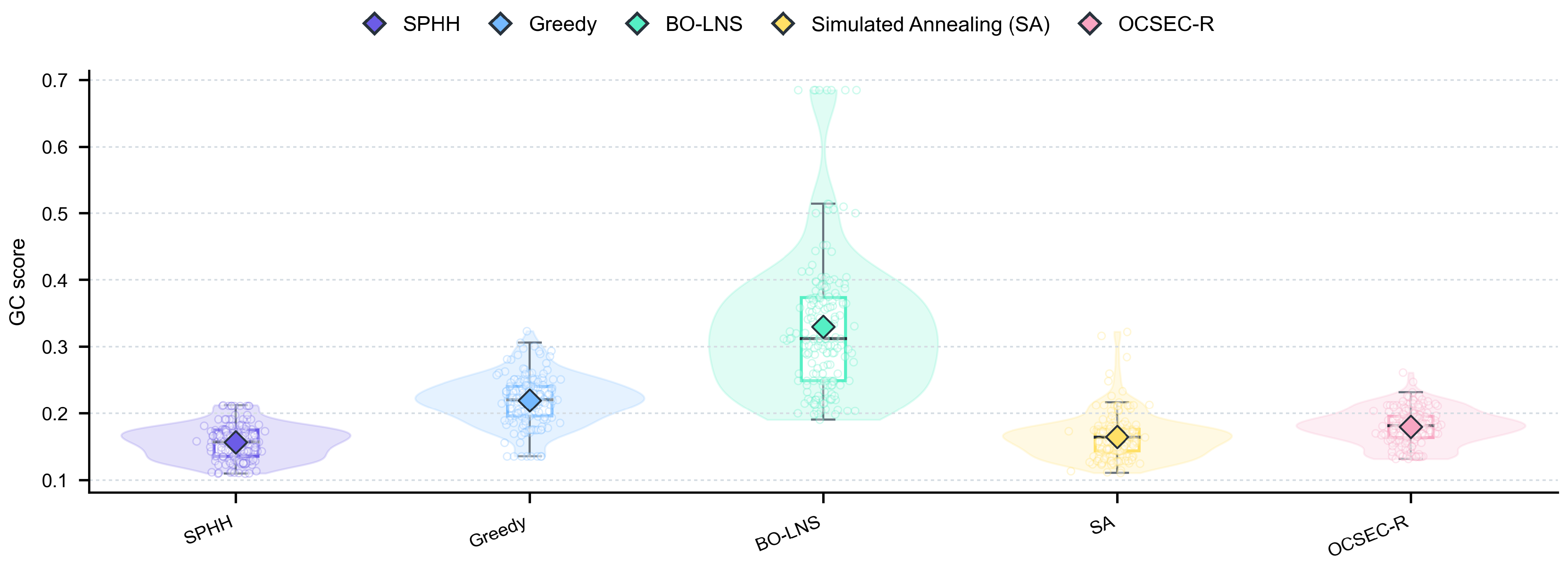
Visual summary. Figure 3 summarizes the 900 formal records using the equal-weight GC score only. The overall distribution is intentionally pooled across all 18 cases, so the broad and sometimes multimodal shapes mainly reflect cross-case difficulty differences rather than a single homogeneous sampling distribution. Within this pooled view, SPHH has the lowest mean marker and the most compact upper tail among the main stochastic competitors, which is consistent with its role as a feasible-incumbent selector. SA is the closest baseline and partially overlaps with SPHH, explaining why the average improvement over SA is positive but moderate. Greedy and BO-LNS show visibly higher centers, and BO-LNS has the widest upper tail because several lean or infeasible-capacity outcomes receive large GC penalties. The figure therefore gives a reader-level overview of the same pattern reported numerically in Table 4 and Table 5: SPHH improves expected GC quality and reduces exposure to poor high-GC outcomes, while the cost of obtaining this protection is reported separately through runtime and resource indicators rather than through additional non-GC boxplot panels.

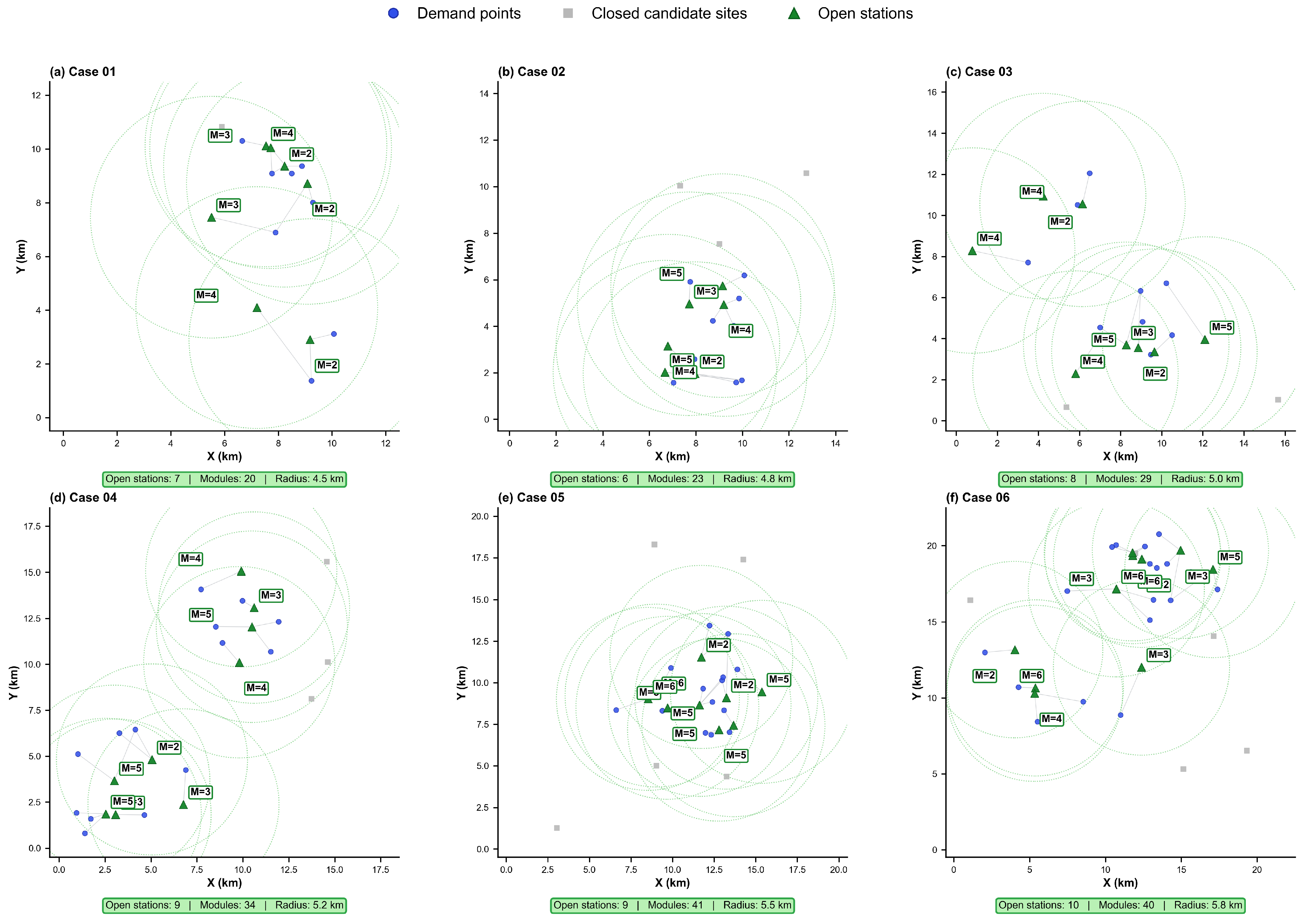
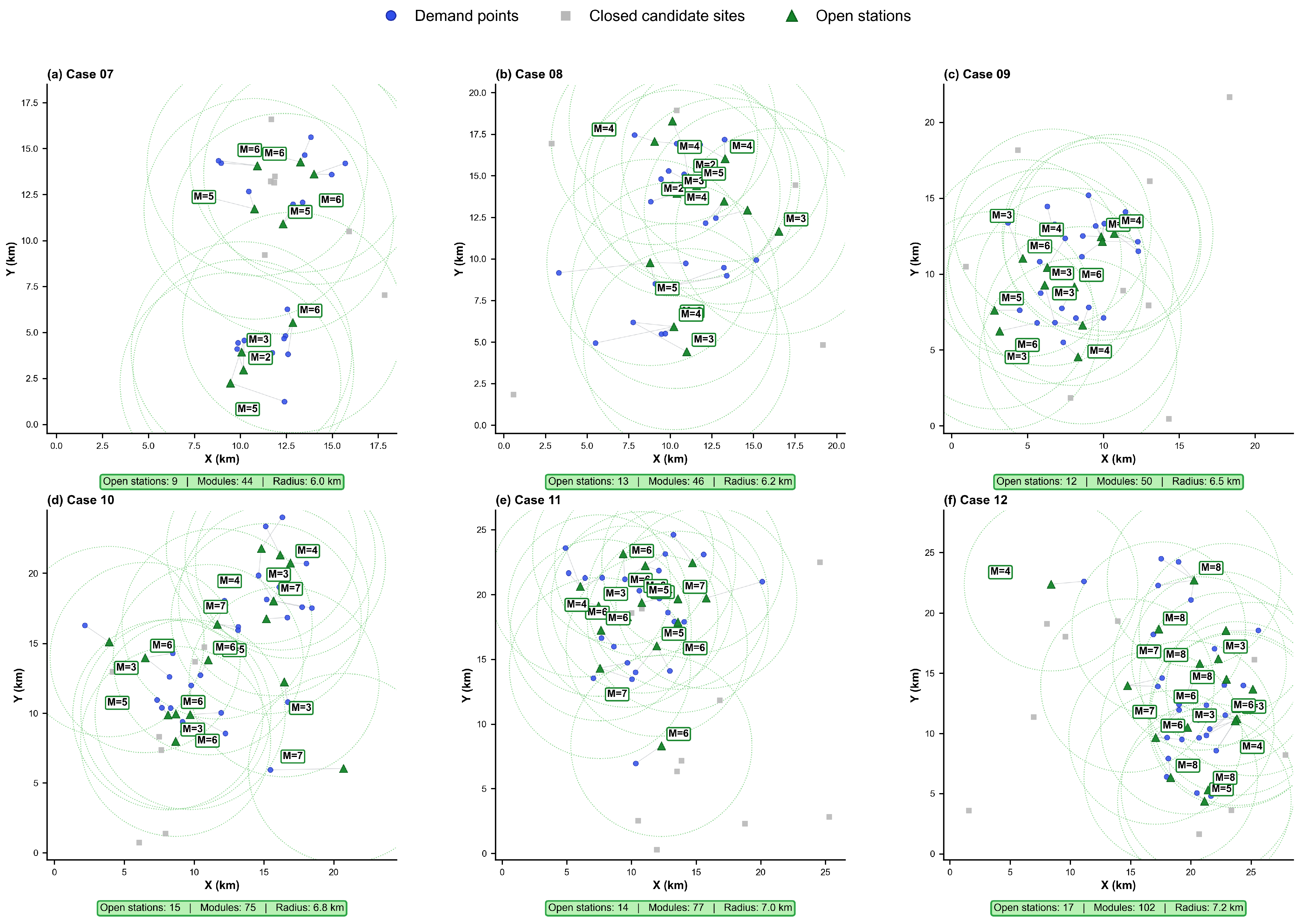
Case-level results. The following scale-specific analyses combine GC score distributions, summary tables for raw components and operations, and spatial layouts. Each GC panel contains 10 independent runs per algorithm and case. The spatial panels display the best feasible SPHH repeat rather than the 10-run mean.

5.6. Small-Scale Cases

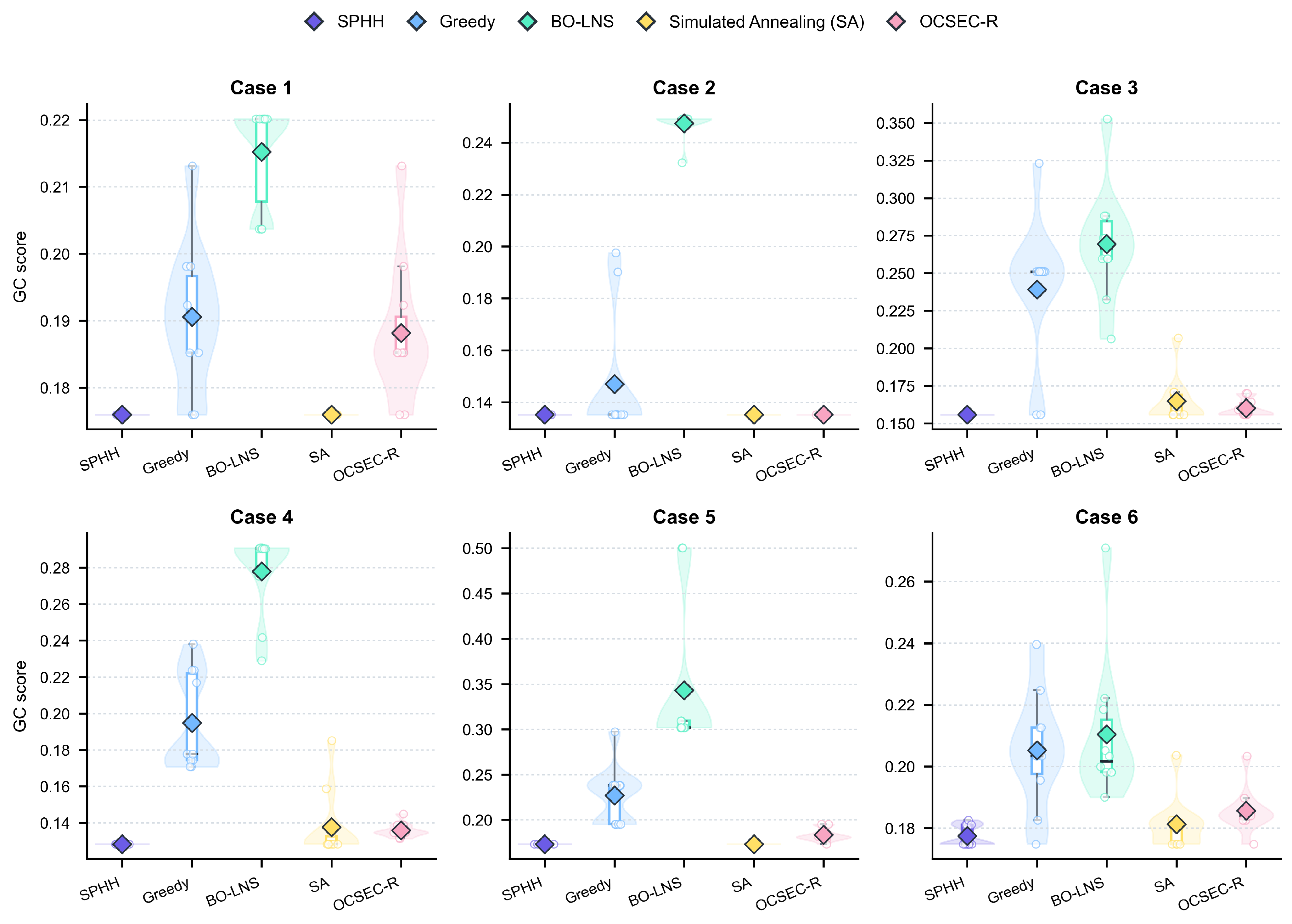
The small-scale cases represent the easier part of the benchmark, where several baselines can still reach high-quality incumbents. Even in this regime, SPHH achieves the lowest mean GC in all six cases: it ties the best baseline in Cases 1, 2, and 5 and strictly improves the best baseline mean in Cases 3, 4, and 6. Averaged across the six cases, SPHH lowers mean GC by 2.38% relative to SA, 4.12% relative to OCSEC-R, 20.30% relative to Greedy, and 37.45% relative to BO-LNS. The detailed per-case mean ± standard deviation results are reported in

Table 6. Small-scale cases: GC and raw objective-component decomposition reported as $\mu \pm \sigma$ over 10 runs.

Case	Algorithm	GC	${\mathit{f}}_1$	${\mathit{f}}_2$	${\mathit{f}}_3$	${\mathit{f}}_4$
1	SPHH	0.1760 ± 0.0000	14.72 ± 0.00	103.694 ± 0.000	572.88 ± 0.00	126.53 ± 0.00
	SA	0.1760 ± 0.0000	14.72 ± 0.00	103.694 ± 0.000	572.88 ± 0.00	126.53 ± 0.00
	OCSEC-R	0.1882 ± 0.0110	14.33 ± 0.66	116.028 ± 18.956	587.67 ± 11.01	110.79 ± 33.17
	Greedy	0.1906 ± 0.0111	14.07 ± 0.72	125.935 ± 21.210	581.90 ± 17.70	95.46 ± 36.06
	BO-LNS	0.2152 ± 0.0080	13.91 ± 0.41	155.386 ± 11.960	561.78 ± 3.76	89.16 ± 0.00
2	SPHH	0.1353 ± 0.0000	14.93 ± 0.00	204.479 ± 0.000	687.63 ± 0.00	56.15 ± 0.00
	SA	0.1353 ± 0.0000	14.93 ± 0.00	204.479 ± 0.000	687.63 ± 0.00	56.15 ± 0.00
	OCSEC-R	0.1353 ± 0.0000	14.93 ± 0.00	204.479 ± 0.000	687.63 ± 0.00	56.15 ± 0.00
	Greedy	0.1470 ± 0.0248	14.86 ± 0.19	212.864 ± 17.750	691.22 ± 8.27	56.15 ± 0.00
	BO-LNS	0.2475 ± 0.0053	17.09 ± 0.62	244.746 ± 15.849	698.15 ± 2.80	67.84 ± 8.02
3	SPHH	0.1559 ± 0.0000	19.35 ± 0.00	241.156 ± 0.000	942.16 ± 0.00	23.76 ± 0.00
	SA	0.1648 ± 0.0161	19.68 ± 0.58	241.156 ± 0.000	942.16 ± 0.00	24.78 ± 2.29
	OCSEC-R	0.1602 ± 0.0058	19.51 ± 0.22	241.156 ± 0.000	942.16 ± 0.00	23.76 ± 0.00
	Greedy	0.2392 ± 0.0493	20.02 ± 0.35	262.991 ± 17.822	963.54 ± 11.31	54.70 ± 16.31
	BO-LNS	0.2693 ± 0.0384	21.19 ± 0.52	278.255 ± 20.704	947.31 ± 8.65	30.26 ± 11.79
4	SPHH	0.1284 ± 0.0000	25.33 ± 0.00	333.476 ± 0.000	1421.58 ± 0.00	88.96 ± 0.00
	SA	0.1377 ± 0.0193	26.03 ± 1.42	330.456 ± 6.367	1422.04 ± 0.96	95.75 ± 17.15
	OCSEC-R	0.1359 ± 0.0040	25.84 ± 0.27	333.476 ± 0.000	1421.58 ± 0.00	89.00 ± 0.12
	Greedy	0.1949 ± 0.0271	24.44 ± 1.05	396.191 ± 29.189	1469.41 ± 23.15	53.66 ± 46.03
	BO-LNS	0.2779 ± 0.0231	29.23 ± 0.84	396.961 ± 12.826	1468.21 ± 7.83	139.44 ± 22.80
5	SPHH	0.1732 ± 0.0000	31.37 ± 0.00	534.159 ± 0.000	1435.64 ± 0.00	212.68 ± 0.00
	SA	0.1732 ± 0.0000	31.37 ± 0.00	534.159 ± 0.000	1435.64 ± 0.00	212.68 ± 0.00
	OCSEC-R	0.1833 ± 0.0071	31.36 ± 1.27	545.356 ± 23.606	1449.69 ± 29.62	191.50 ± 44.67
	Greedy	0.2268 ± 0.0328	29.76 ± 1.20	609.241 ± 21.717	1512.07 ± 29.74	138.69 ± 51.44
	BO-LNS	0.3431 ± 0.0828	34.20 ± 4.59	639.376 ± 99.683	1734.28 ± 560.15	222.85 ± 121.81
6	SPHH	0.1774 ± 0.0035	40.87 ± 1.39	640.490 ± 22.285	2399.65 ± 6.88	233.66 ± 76.87
	SA	0.1813 ± 0.0087	41.17 ± 1.35	644.697 ± 19.246	2397.55 ± 7.74	227.12 ± 63.67
	OCSEC-R	0.1856 ± 0.0073	41.33 ± 0.94	654.211 ± 23.512	2390.87 ± 5.10	219.96 ± 44.53
	Greedy	0.2053 ± 0.0189	38.97 ± 1.68	711.529 ± 39.350	2444.62 ± 74.84	158.94 ± 71.24
	BO-LNS	0.2104 ± 0.0234	43.73 ± 1.47	661.160 ± 18.430	2396.73 ± 20.77	227.51 ± 48.70

Note: Bold values indicate the most favorable value for each reported metric within the corresponding comparison group.

and

Table 7. Small-scale cases: operational indicators reported as $\mu \pm \sigma$ over 10 runs.

Case	Algorithm	Time (s)	Open	Modules	Wait (${10}^{-3}$ h)	Queue (${10}^{-3}$)	Util. (%)	Conv. Iter.
1	SPHH	28.6 ± 3.9	7.0 ± 0.0	20.0 ± 0.0	1.66 ± 0.00	5.08 ± 0.00	10.5 ± 0.0	3021 ± 6
	SA	2.9 ± 0.1	7.0 ± 0.0	20.0 ± 0.0	1.66 ± 0.00	5.08 ± 0.00	10.5 ± 0.0	1875 ± 347
	OCSEC-R	7.7 ± 0.9	6.1 ± 0.6	17.6 ± 1.5	1.68 ± 0.41	5.21 ± 1.13	11.6 ± 0.8	0 ± 1
	Greedy	4.3 ± 0.7	6.1 ± 0.6	18.0 ± 1.5	1.47 ± 0.43	4.64 ± 1.19	11.2 ± 0.8	4 ± 2
	BO-LNS	10.1 ± 1.4	5.3 ± 0.5	13.6 ± 1.0	1.66 ± 0.13	5.26 ± 0.43	13.0 ± 0.8	5 ± 4
2	SPHH	31.8 ± 3.0	6.0 ± 0.0	23.0 ± 0.0	0.73 ± 0.00	2.39 ± 0.00	10.2 ± 0.0	3022 ± 4
	SA	3.2 ± 0.1	6.0 ± 0.0	23.0 ± 0.0	0.73 ± 0.00	2.39 ± 0.00	10.2 ± 0.0	1964 ± 311
	OCSEC-R	9.5 ± 1.2	6.0 ± 0.0	23.0 ± 0.0	0.73 ± 0.00	2.39 ± 0.00	10.2 ± 0.0	31 ± 97
	Greedy	4.8 ± 0.9	5.8 ± 0.4	22.3 ± 1.5	0.76 ± 0.06	2.48 ± 0.20	10.5 ± 0.7	3 ± 2
	BO-LNS	11.0 ± 1.1	5.1 ± 0.3	14.0 ± 0.0	1.41 ± 0.16	4.59 ± 0.36	15.0 ± 0.0	54 ± 62
3	SPHH	36.3 ± 1.2	8.0 ± 0.0	29.0 ± 0.0	0.57 ± 0.00	1.71 ± 0.00	9.8 ± 0.0	3026 ± 7
	SA	3.7 ± 0.3	8.0 ± 0.0	28.0 ± 1.6	0.60 ± 0.06	1.83 ± 0.27	10.1 ± 0.5	1679 ± 792
	OCSEC-R	11.6 ± 1.1	8.0 ± 0.0	28.0 ± 1.2	0.58 ± 0.00	1.71 ± 0.01	9.9 ± 0.2	211 ± 203
	Greedy	6.6 ± 0.3	7.1 ± 0.6	25.3 ± 2.5	0.99 ± 0.23	3.13 ± 0.77	11.6 ± 1.2	3 ± 2
	BO-LNS	10.3 ± 0.5	7.1 ± 0.6	19.3 ± 1.4	1.01 ± 0.16	2.75 ± 0.64	13.0 ± 1.0	108 ± 143
4	SPHH	42.0 ± 2.4	9.0 ± 0.0	34.0 ± 0.0	0.58 ± 0.00	2.00 ± 0.00	9.8 ± 0.0	3026 ± 4
	SA	10.1 ± 6.4	9.0 ± 0.0	32.6 ± 2.8	0.68 ± 0.22	2.33 ± 0.73	10.3 ± 1.0	1657 ± 948
	OCSEC-R	12.8 ± 0.9	9.0 ± 0.0	31.8 ± 0.9	0.59 ± 0.03	2.02 ± 0.04	10.1 ± 0.2	464 ± 913
	Greedy	7.1 ± 0.6	7.6 ± 0.5	29.3 ± 2.0	0.45 ± 0.34	1.57 ± 1.19	10.9 ± 1.0	4 ± 2
	BO-LNS	12.3 ± 1.6	7.1 ± 0.3	19.7 ± 1.3	1.71 ± 0.37	5.68 ± 1.17	16.0 ± 1.0	44 ± 63
5	SPHH	44.4 ± 0.9	9.0 ± 0.0	41.0 ± 0.0	1.16 ± 0.00	4.20 ± 0.00	12.0 ± 0.0	3341 ± 978
	SA	19.0 ± 6.3	9.0 ± 0.0	41.0 ± 0.0	1.16 ± 0.00	4.20 ± 0.00	12.0 ± 0.0	2427 ± 96
	OCSEC-R	13.6 ± 0.8	8.8 ± 0.4	38.0 ± 1.4	1.07 ± 0.21	3.87 ± 0.73	12.3 ± 0.3	158 ± 193
	Greedy	7.2 ± 0.4	7.6 ± 0.5	35.7 ± 3.3	0.91 ± 0.33	3.39 ± 1.22	13.1 ± 1.2	7 ± 3
	BO-LNS	12.8 ± 0.7	7.0 ± 1.6	23.4 ± 1.3	1.75 ± 0.91	6.30 ± 2.94	18.4 ± 1.0	259 ± 315
6	SPHH	55.7 ± 2.1	10.3 ± 0.5	40.0 ± 1.2	1.29 ± 0.30	4.87 ± 0.90	14.1 ± 0.2	3660 ± 1297
	SA	21.2 ± 6.5	10.2 ± 0.4	38.7 ± 2.3	1.31 ± 0.25	4.89 ± 0.76	14.3 ± 0.5	2316 ± 633
	OCSEC-R	18.8 ± 1.8	10.0 ± 0.5	36.5 ± 1.8	1.34 ± 0.15	4.87 ± 0.49	14.7 ± 0.4	112 ± 167
	Greedy	11.1 ± 0.7	9.0 ± 0.7	36.8 ± 1.5	0.99 ± 0.39	4.11 ± 1.23	14.9 ± 0.6	6 ± 2
	BO-LNS	14.2 ± 0.7	9.9 ± 0.3	30.9 ± 2.3	1.52 ± 0.35	5.60 ± 1.40	16.3 ± 1.2	297 ± 359

Note: Bold values indicate the most favorable value for each reported metric within the corresponding comparison group.

.

The gains in Cases 3, 4, and 6 are useful because they show that SPHH does not improve the GC score through a single repeated mechanism. In Case 3, SPHH reaches a lower GC than SA while reducing construction and queue-related terms and preserving the same degradation and travel components. In Case 4, SPHH accepts a slightly higher degradation component than SA, but the lower construction and queue burden keeps the weighted GC smaller. In Case 6, the improvement is again different: the degradation reduction is sufficient to offset small increases in travel and queue terms. These examples show that SPHH acts as a case-level selector of balanced solutions, rather than as a heuristic that simply minimizes one component.

The operational indicators also separate compact layouts from high-quality layouts. Greedy and BO-LNS often open fewer stations or install fewer modules, but those resource savings do not translate into better GC values. BO-LNS is the clearest example: it uses the leanest capacity on several small cases, yet its average GC is 0.2606 compared with 0.1577 for SPHH. SPHH therefore pays additional offline runtime to preserve feasible incumbents with lower balanced cost and lower run-to-run variation; its average within-case GC standard deviation is 0.0006, compared with 0.0073 for SA and substantially larger spreads for the less stable baselines.

Figure 4 and Figure 5 make these case-level results concrete before the complete numerical summary: the former compares the 10-run GC distributions, whereas the latter shows the best feasible SPHH spatial configuration for each small-scale case.

5.7. Medium-Scale Cases

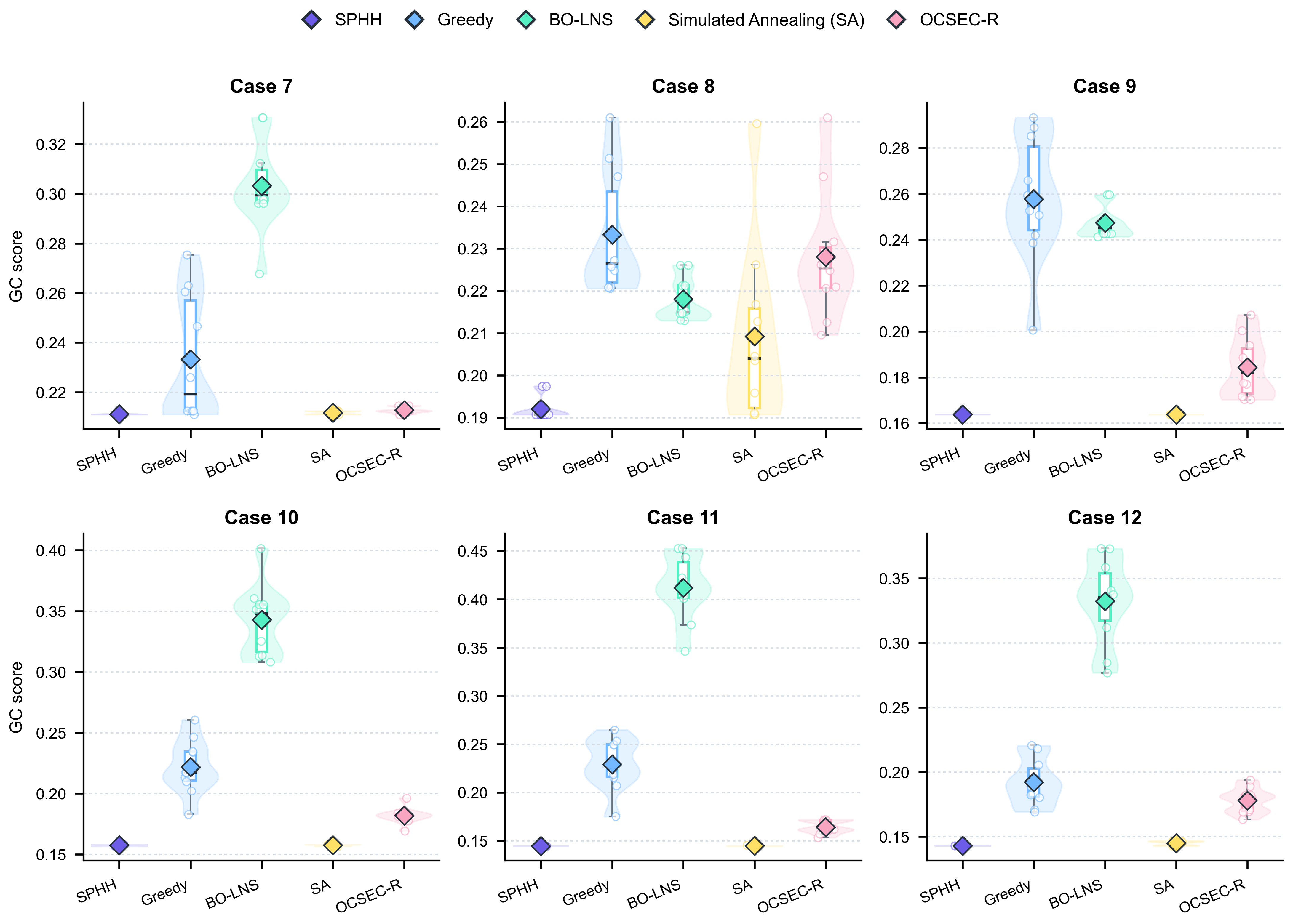
The medium-scale cases form a transition zone between easy and difficult search instances. The annealing baseline remains competitive in several cases, but SPHH starts to show a clearer advantage in expected GC value as the demand and candidate-site sets become larger. In this group, SPHH strictly improves the best baseline mean in five cases and ties in the remaining one, Case 9. Its average GC reduction is 1.65% relative to SA, 12.09% relative to OCSEC-R, 25.85% relative to Greedy, and 42.00% relative to BO-LNS. The detailed per-case mean±standard deviation results are reported in

Table 8. Medium-scale cases: GC and raw objective-component decomposition reported as $\mu \pm \sigma$ over 10 runs.

Case	Algorithm	GC	${\mathit{f}}_1$	${\mathit{f}}_2$	${\mathit{f}}_3$	${\mathit{f}}_4$
7	SPHH	0.2112 ± 0.0004	48.06 ± 0.65	720.536 ± 14.466	2034.03 ± 7.26	127.31 ± 38.72
	SA	0.2117 ± 0.0007	47.24 ± 1.09	738.834 ± 24.110	2024.84 ± 12.11	78.32 ± 64.54
	OCSEC-R	0.2128 ± 0.0014	46.72 ± 0.83	752.558 ± 19.288	2017.95 ± 9.69	41.59 ± 51.63
	Greedy	0.2332 ± 0.0256	46.25 ± 0.98	763.353 ± 17.813	2099.13 ± 100.44	28.09 ± 39.45
	BO-LNS	0.3033 ± 0.0183	47.65 ± 2.27	870.621 ± 50.744	2172.79 ± 58.81	24.90 ± 9.27
8	SPHH	0.1921 ± 0.0028	61.30 ± 2.58	668.095 ± 44.504	3256.73 ± 4.44	242.13 ± 107.56
	SA	0.2092 ± 0.0215	62.01 ± 1.26	696.989 ± 37.151	3240.57 ± 52.25	225.19 ± 99.26
	OCSEC-R	0.2281 ± 0.0155	57.24 ± 0.87	815.746 ± 22.258	3198.21 ± 93.31	60.25 ± 37.33
	Greedy	0.2333 ± 0.0146	57.18 ± 1.36	806.948 ± 26.707	3254.23 ± 80.60	81.10 ± 57.95
	BO-LNS	0.2180 ± 0.0052	59.89 ± 0.84	781.221 ± 6.993	3141.49 ± 8.37	83.14 ± 19.72
9	SPHH	0.1638 ± 0.0000	65.35 ± 0.00	802.335 ± 0.000	2504.98 ± 0.00	67.15 ± 0.00
	SA	0.1638 ± 0.0000	65.35 ± 0.00	802.335 ± 0.000	2504.98 ± 0.00	67.15 ± 0.00
	OCSEC-R	0.1844 ± 0.0131	67.89 ± 1.49	802.335 ± 0.000	2504.98 ± 0.00	84.14 ± 27.24
	Greedy	0.2578 ± 0.0279	64.22 ± 1.84	915.838 ± 38.359	2845.28 ± 207.75	88.14 ± 19.55
	BO-LNS	0.2474 ± 0.0069	67.47 ± 0.80	911.446 ± 1.270	2586.29 ± 4.24	89.71 ± 11.20
10	SPHH	0.1575 ± 0.0006	75.07 ± 1.35	1005.958 ± 7.416	3600.43 ± 20.57	45.71 ± 15.74
	SA	0.1576 ± 0.0006	75.33 ± 1.32	1004.551 ± 7.266	3596.53 ± 20.15	48.70 ± 15.42
	OCSEC-R	0.1817 ± 0.0067	75.61 ± 1.54	1071.530 ± 5.298	3592.56 ± 53.57	32.34 ± 3.05
	Greedy	0.2219 ± 0.0226	72.70 ± 2.43	1126.968 ± 40.543	3844.96 ± 129.52	39.37 ± 22.25
	BO-LNS	0.3430 ± 0.0286	75.72 ± 4.87	1271.179 ± 88.624	4287.43 ± 177.60	165.16 ± 135.17
11	SPHH	0.1447 ± 0.0000	79.33 ± 0.00	1210.135 ± 0.000	3226.66 ± 0.00	6.52 ± 0.00
	SA	0.1448 ± 0.0003	79.34 ± 0.05	1210.135 ± 0.000	3226.66 ± 0.00	6.52 ± 0.00
	OCSEC-R	0.1643 ± 0.0067	83.03 ± 1.34	1210.135 ± 0.000	3228.91 ± 7.11	8.53 ± 1.37
	Greedy	0.2292 ± 0.0266	78.47 ± 1.29	1306.045 ± 52.573	3570.29 ± 111.46	5.59 ± 2.69
	BO-LNS	0.4122 ± 0.0339	80.42 ± 3.45	1506.070 ± 61.891	4188.19 ± 234.93	84.14 ± 86.14
12	SPHH	0.1430 ± 0.0001	90.12 ± 0.04	1309.637 ± 0.000	4875.65 ± 0.00	98.76 ± 0.00
	SA	0.1449 ± 0.0017	89.11 ± 2.69	1332.601 ± 36.985	4872.78 ± 13.54	85.18 ± 21.88
	OCSEC-R	0.1779 ± 0.0097	90.69 ± 6.28	1415.562 ± 71.022	4920.52 ± 101.54	86.07 ± 33.19
	Greedy	0.1923 ± 0.0180	84.65 ± 3.00	1493.496 ± 55.829	5099.06 ± 143.65	61.13 ± 33.50
	BO-LNS	0.3321 ± 0.0330	97.35 ± 2.94	1631.325 ± 42.026	5669.13 ± 257.22	221.21 ± 96.21

Note: Bold values indicate the most favorable value for each reported metric within the corresponding comparison group.

and

Table 9. Medium-scale cases: operational indicators reported as $\mu \pm \sigma$ over 10 runs.

Case	Algorithm	Time (s)	Open	Modules	Wait (${10}^{-3}$ h)	Queue (${10}^{-3}$)	Util. (%)	Conv. Iter.
7	SPHH	56.6 ± 3.0	8.9 ± 0.3	43.7 ± 0.9	0.52 ± 0.13	2.29 ± 0.49	12.9 ± 0.2	3051 ± 23
	SA	25.5 ± 4.9	8.5 ± 0.5	42.5 ± 1.6	0.35 ± 0.22	1.67 ± 0.82	13.1 ± 0.3	2581 ± 110
	OCSEC-R	18.0 ± 1.1	8.2 ± 0.4	41.3 ± 1.5	0.23 ± 0.17	1.20 ± 0.65	13.4 ± 0.3	411 ± 665
	Greedy	10.6 ± 0.9	8.1 ± 0.3	41.1 ± 1.5	0.18 ± 0.14	1.01 ± 0.55	13.3 ± 0.5	6 ± 2
	BO-LNS	15.1 ± 0.8	6.5 ± 0.7	29.5 ± 0.8	0.28 ± 0.08	1.77 ± 0.49	18.1 ± 0.5	99 ± 139
8	SPHH	71.4 ± 1.5	12.6 ± 0.8	45.4 ± 1.3	0.71 ± 0.25	3.22 ± 0.92	13.3 ± 0.1	3355 ± 963
	SA	16.3 ± 10.0	12.5 ± 0.5	43.2 ± 2.5	0.72 ± 0.24	3.36 ± 0.88	13.7 ± 0.7	2044 ± 634
	OCSEC-R	23.3 ± 1.0	10.2 ± 0.6	38.2 ± 2.1	0.40 ± 0.13	2.12 ± 0.44	14.8 ± 0.9	55 ± 145
	Greedy	15.7 ± 1.2	10.0 ± 0.7	38.8 ± 2.0	0.40 ± 0.15	2.24 ± 0.54	15.0 ± 0.8	6 ± 4
	BO-LNS	17.1 ± 0.5	10.0 ± 0.0	35.5 ± 1.0	0.61 ± 0.13	3.04 ± 0.47	16.3 ± 0.4	323 ± 349
9	SPHH	80.5 ± 1.9	12.0 ± 0.0	50.0 ± 0.0	0.37 ± 0.00	2.29 ± 0.00	14.1 ± 0.0	3024 ± 5
	SA	7.2 ± 0.3	12.0 ± 0.0	50.0 ± 0.0	0.37 ± 0.00	2.29 ± 0.00	14.1 ± 0.0	2475 ± 179
	OCSEC-R	27.0 ± 0.7	12.0 ± 0.0	43.8 ± 2.7	0.48 ± 0.15	2.66 ± 0.48	15.1 ± 0.6	707 ± 721
	Greedy	17.9 ± 0.5	9.9 ± 0.7	41.8 ± 3.9	0.48 ± 0.10	3.16 ± 0.61	16.6 ± 1.4	6 ± 3
	BO-LNS	18.5 ± 1.2	10.0 ± 0.0	35.3 ± 0.8	0.62 ± 0.07	3.43 ± 0.28	17.8 ± 0.3	514 ± 381
10	SPHH	90.2 ± 3.2	15.0 ± 0.0	73.5 ± 1.6	0.17 ± 0.04	0.99 ± 0.27	11.2 ± 0.4	3061 ± 10
	SA	8.3 ± 0.2	15.0 ± 0.0	73.2 ± 1.5	0.18 ± 0.04	1.04 ± 0.27	11.3 ± 0.4	2845 ± 111
	OCSEC-R	28.0 ± 1.0	13.9 ± 0.3	61.6 ± 3.9	0.17 ± 0.06	0.90 ± 0.13	12.5 ± 0.4	199 ± 235
	Greedy	18.7 ± 1.0	12.7 ± 0.7	63.4 ± 1.5	0.17 ± 0.06	1.05 ± 0.36	12.8 ± 0.3	11 ± 4
	BO-LNS	21.0 ± 1.6	9.9 ± 1.3	42.2 ± 2.0	0.68 ± 0.33	3.34 ± 1.30	18.3 ± 0.9	912 ± 1078
11	SPHH	98.1 ± 6.0	14.0 ± 0.0	77.0 ± 0.0	0.05 ± 0.00	0.38 ± 0.00	11.2 ± 0.0	3054 ± 9
	SA	8.8 ± 0.3	14.0 ± 0.0	76.9 ± 0.3	0.05 ± 0.00	0.38 ± 0.00	11.2 ± 0.0	2773 ± 111
	OCSEC-R	30.4 ± 1.2	14.0 ± 0.0	66.8 ± 3.2	0.12 ± 0.04	0.53 ± 0.09	12.4 ± 0.4	1051 ± 940
	Greedy	20.7 ± 1.7	12.3 ± 0.9	66.6 ± 3.7	0.06 ± 0.02	0.42 ± 0.14	12.7 ± 0.8	13 ± 3
	BO-LNS	23.5 ± 3.0	9.0 ± 0.8	43.8 ± 1.3	0.38 ± 0.24	2.17 ± 0.98	19.1 ± 0.5	407 ± 729
12	SPHH	98.4 ± 8.5	17.0 ± 0.0	101.9 ± 0.3	0.21 ± 0.00	1.46 ± 0.00	10.7 ± 0.0	3677 ± 1281
	SA	9.9 ± 0.4	16.7 ± 0.5	99.2 ± 2.6	0.19 ± 0.04	1.31 ± 0.26	10.8 ± 0.3	2948 ± 47
	OCSEC-R	28.4 ± 2.2	15.4 ± 1.6	83.0 ± 6.1	0.25 ± 0.11	1.46 ± 0.45	12.1 ± 0.8	163 ± 224
	Greedy	16.5 ± 1.3	13.6 ± 0.8	85.2 ± 3.2	0.17 ± 0.07	1.15 ± 0.48	12.0 ± 0.5	19 ± 3
	BO-LNS	22.3 ± 1.5	11.2 ± 0.6	48.3 ± 2.8	0.81 ± 0.23	4.59 ± 1.20	19.7 ± 1.0	1388 ± 1132

Note: Bold values indicate the most favorable value for each reported metric within the corresponding comparison group.

.

The medium-scale gains are informative at different effect sizes. Case 8 shows the largest reduction over SA, with SPHH lowering the mean GC by 8.18%; this improvement is associated with lower construction and degradation components while maintaining a feasible travel–queue trade-off. Cases 10 and 11 show much smaller numerical gains, but they are still important because they indicate that SPHH can retain a marginally better incumbent when SA is already very close. Case 12 illustrates a different mechanism: SPHH accepts slightly higher construction, travel, and queue components than SA, but the reduction in degradation cost is large enough to produce a lower weighted GC. Thus, the dominant improvement mechanism is not fixed across cases.

Another important observation is that the medium-scale cases begin to separate fast but less reliable heuristics from slower but more reliable ones. Greedy remains attractive in runtime and convergence iteration, and BO-LNS often uses fewer modules, but both algorithms produce substantially higher expected GC values. OCSEC-R is competitive on selected structural sub-costs, especially when it reduces travel or queue terms at particular sites, but its full weighted objective remains above SPHH in every medium-scale case. Therefore, the evidence suggests that the core planning difficulty is no longer merely finding a feasible network; it is stabilizing the balance among capacity cost, degradation pressure, travel burden, and queue severity under repeated stochastic search.

Figure 6 and Figure 7 make these case-level trade-offs concrete before the complete numerical summary: the former compares the 10-run GC distributions, whereas the latter shows the best feasible SPHH spatial configuration for each medium-scale case.

5.8. Large-Scale Cases

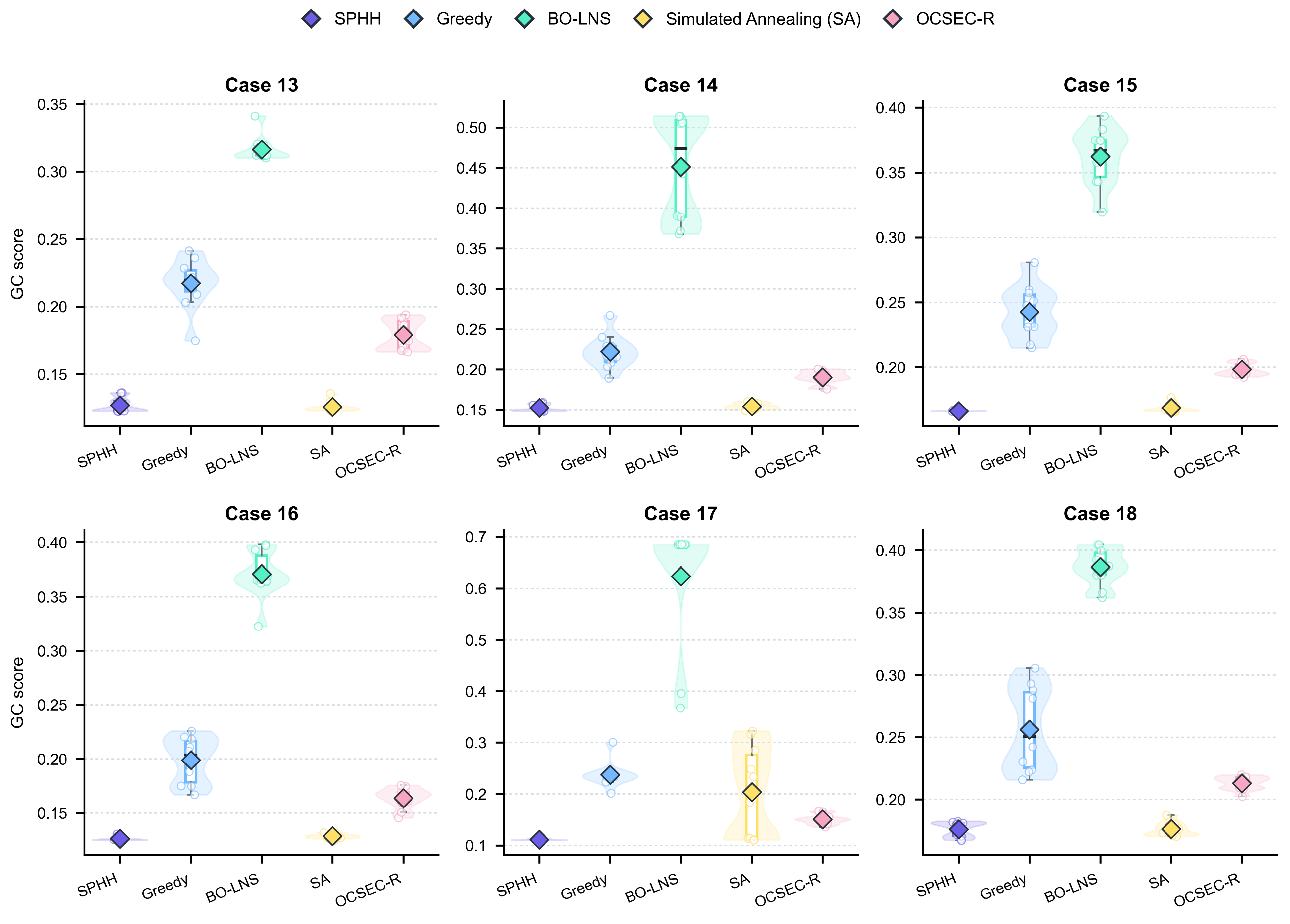
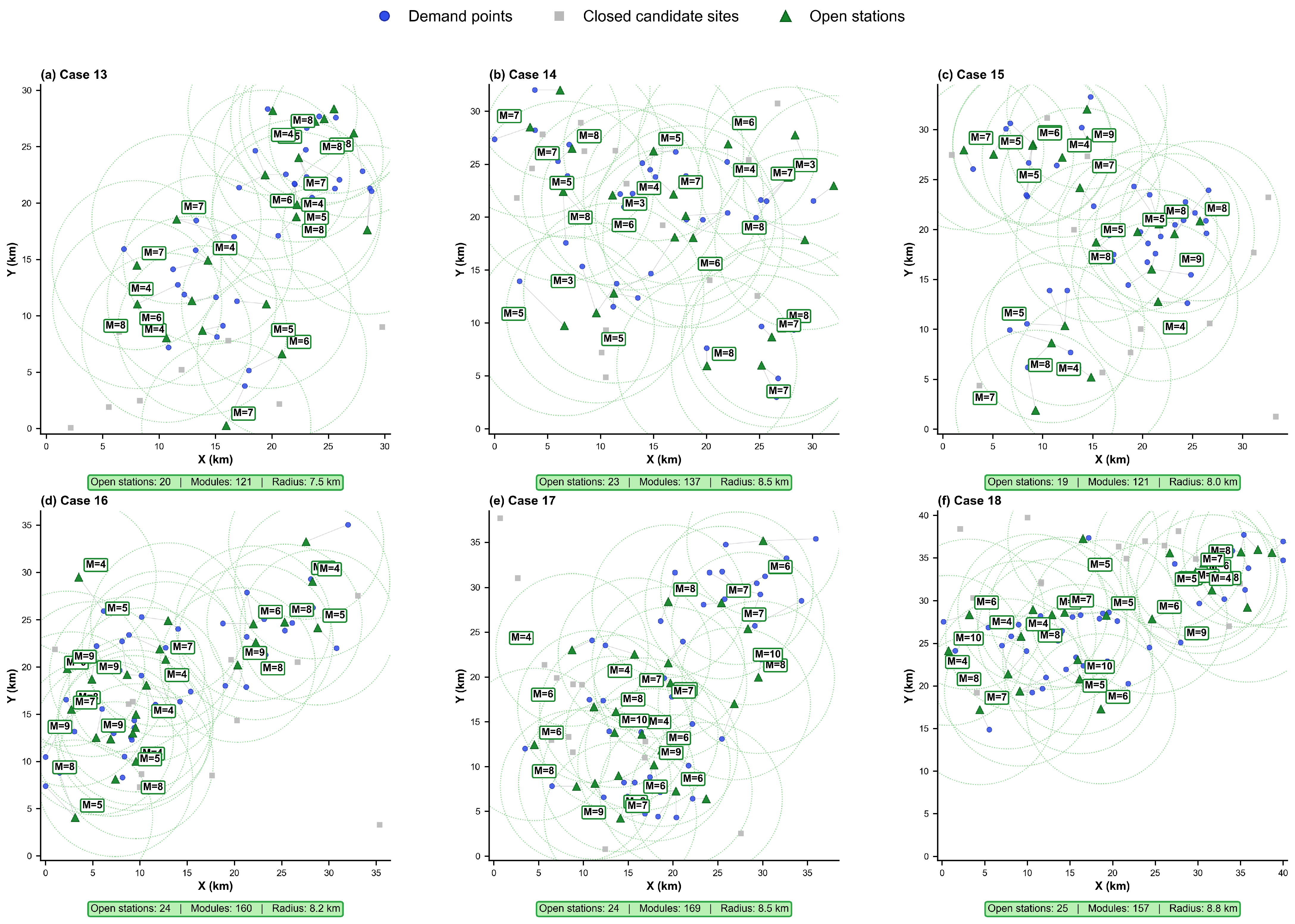
The large-scale cases are the stress-test regime of the benchmark. Here, SPHH shows its clearest advantage, but it also reveals a useful boundary condition. SPHH strictly improves the best baseline mean in five cases, while SA remains slightly better in Case 13 by 0.95%. Across the six large cases, SPHH reduces mean GC by 8.24% relative to SA, 21.92% relative to OCSEC-R, 37.58% relative to Greedy, and 63.82% relative to BO-LNS. The detailed per-case mean±standard deviation results are reported in

Table 10. Large-scale cases: GC and raw objective-component decomposition reported as $\mu \pm \sigma$ over 10 runs.

Case	Algorithm	GC	${\mathit{f}}_1$	${\mathit{f}}_2$	${\mathit{f}}_3$	${\mathit{f}}_4$
13	SPHH	0.1270 ± 0.0056	119.51 ± 1.30	1416.448 ± 41.068	6128.92 ± 33.08	10.77 ± 9.31
	SA	0.1258 ± 0.0040	119.81 ± 1.21	1400.550 ± 36.105	6148.63 ± 33.22	8.58 ± 6.98
	OCSEC-R	0.1790 ± 0.0110	128.78 ± 7.16	1525.172 ± 53.473	6197.29 ± 229.75	13.94 ± 6.94
	Greedy	0.2172 ± 0.0188	114.18 ± 3.49	1726.502 ± 87.724	7072.33 ± 247.99	4.72 ± 3.36
	BO-LNS	0.3163 ± 0.0095	128.51 ± 2.90	1939.302 ± 40.575	7267.88 ± 171.52	96.83 ± 34.43
14	SPHH	0.1523 ± 0.0045	134.41 ± 2.59	1237.197 ± 89.249	6930.13 ± 60.22	73.74 ± 18.66
	SA	0.1544 ± 0.0037	135.67 ± 2.77	1221.567 ± 71.598	6954.86 ± 39.90	76.27 ± 16.84
	OCSEC-R	0.1900 ± 0.0084	139.01 ± 4.96	1428.409 ± 67.926	6912.26 ± 113.46	21.94 ± 17.52
	Greedy	0.2221 ± 0.0215	128.74 ± 2.20	1420.203 ± 78.317	7557.61 ± 216.65	24.99 ± 17.71
	BO-LNS	0.4511 ± 0.0650	133.00 ± 14.58	2080.171 ± 285.473	9887.21 ± 1655.07	137.39 ± 157.33
15	SPHH	0.1660 ± 0.0004	142.40 ± 0.15	1981.437 ± 0.000	7748.48 ± 0.00	5.01 ± 0.00
	SA	0.1686 ± 0.0036	145.23 ± 4.12	1956.199 ± 40.776	7762.05 ± 22.03	12.52 ± 13.58
	OCSEC-R	0.1981 ± 0.0049	153.08 ± 2.38	2024.944 ± 30.023	7711.78 ± 25.32	8.73 ± 6.44
	Greedy	0.2425 ± 0.0206	143.13 ± 2.11	2156.786 ± 76.286	8387.17 ± 291.42	12.28 ± 12.20
	BO-LNS	0.3624 ± 0.0223	152.73 ± 9.36	2494.134 ± 189.757	8988.36 ± 311.99	73.87 ± 105.76
16	SPHH	0.1262 ± 0.0019	164.58 ± 0.84	1770.056 ± 0.000	7804.37 ± 33.40	6.76 ± 0.00
	SA	0.1286 ± 0.0022	168.39 ± 3.77	1739.090 ± 45.860	7790.20 ± 8.34	25.28 ± 26.04
	OCSEC-R	0.1636 ± 0.0097	183.20 ± 10.88	1794.574 ± 46.088	7855.62 ± 155.88	17.91 ± 10.69
	Greedy	0.1988 ± 0.0212	160.35 ± 5.31	2081.827 ± 113.166	8663.00 ± 280.44	16.25 ± 18.99
	BO-LNS	0.3707 ± 0.0222	163.34 ± 6.51	2810.716 ± 104.564	10,223.38 ± 381.34	104.17 ± 127.12
17	SPHH	0.1111 ± 0.0012	186.31 ± 0.64	2369.578 ± 0.000	9304.08 ± 0.00	1.26 ± 0.00
	SA	0.2038 ± 0.0881	209.63 ± 21.62	2399.837 ± 56.315	9891.08 ± 680.55	523.19 ± 733.96
	OCSEC-R	0.1506 ± 0.0098	202.56 ± 6.11	2399.310 ± 63.651	9366.63 ± 95.71	8.44 ± 11.41
	Greedy	0.2374 ± 0.0250	179.43 ± 4.59	2768.047 ± 104.384	10,768.01 ± 351.97	1.70 ± 2.44
	BO-LNS	0.6239 ± 0.1280	343.82 ± 77.32	1624.364 ± 839.895	12,482.10 ± 525.22	38,623.50 ± 20,298.57
18	SPHH	0.1760 ± 0.0059	213.38 ± 2.84	2613.100 ± 78.881	7890.90 ± 89.91	40.54 ± 25.77
	SA	0.1762 ± 0.0056	213.52 ± 3.59	2615.231 ± 95.705	7873.27 ± 129.33	56.75 ± 34.14
	OCSEC-R	0.2130 ± 0.0055	222.99 ± 6.71	2814.307 ± 1.035	7730.75 ± 287.69	36.68 ± 35.42
	Greedy	0.2561 ± 0.0335	204.64 ± 4.92	2977.591 ± 124.782	9067.07 ± 690.95	31.28 ± 23.58
	BO-LNS	0.3866 ± 0.0147	204.87 ± 3.62	3590.081 ± 105.040	10,548.89 ± 420.96	46.48 ± 78.93

Note: Bold values indicate the most favorable value for each reported metric within the corresponding comparison group.

and

Table 11. Large-scale cases: operational indicators reported as $\mu \pm \sigma$ over 10 runs.

Case	Algorithm	Time (s)	Open	Modules	Wait (${10}^{-3}$ h)	Queue (${10}^{-3}$)	Util. (%)	Conv. Iter.
13	SPHH	139.2 ± 3.6	19.8 ± 0.4	117.1 ± 2.8	0.03 ± 0.02	0.27 ± 0.11	8.8 ± 0.2	4593 ± 1597
	SA	11.0 ± 0.8	19.9 ± 0.3	116.9 ± 1.4	0.03 ± 0.01	0.25 ± 0.09	8.7 ± 0.2	2928 ± 56
	OCSEC-R	42.2 ± 1.3	18.4 ± 1.1	87.6 ± 7.8	0.11 ± 0.06	0.48 ± 0.18	11.0 ± 0.7	682 ± 1051
	Greedy	27.8 ± 0.7	15.2 ± 1.0	93.0 ± 6.3	0.03 ± 0.02	0.23 ± 0.14	10.8 ± 0.7	21 ± 6
	BO-LNS	29.0 ± 2.0	12.5 ± 0.7	57.2 ± 1.2	0.43 ± 0.02	1.90 ± 0.19	16.6 ± 0.6	1243 ± 640
14	SPHH	132.0 ± 11.5	22.5 ± 1.2	130.4 ± 6.8	0.11 ± 0.02	0.78 ± 0.14	8.8 ± 0.2	5817 ± 963
	SA	14.0 ± 0.4	25.3 ± 1.1	138.2 ± 4.9	0.10 ± 0.02	0.72 ± 0.14	8.0 ± 0.4	2956 ± 29
	OCSEC-R	32.2 ± 1.3	20.7 ± 0.8	101.9 ± 11.2	0.14 ± 0.10	0.48 ± 0.18	10.2 ± 0.7	945 ± 1115
	Greedy	16.0 ± 0.8	20.1 ± 1.0	122.4 ± 6.5	0.05 ± 0.03	0.38 ± 0.18	9.1 ± 0.4	35 ± 9
	BO-LNS	32.2 ± 2.1	12.5 ± 2.6	61.1 ± 3.1	0.34 ± 0.33	1.52 ± 1.23	16.4 ± 0.8	804 ± 493
15	SPHH	507.8 ± 1107.7	19.0 ± 0.0	120.7 ± 0.7	0.02 ± 0.00	0.17 ± 0.00	9.8 ± 0.0	3383 ± 961
	SA	15.4 ± 6.0	20.2 ± 1.0	124.1 ± 7.3	0.03 ± 0.02	0.26 ± 0.17	9.6 ± 0.7	2942 ± 44
	OCSEC-R	51.3 ± 3.1	19.0 ± 0.0	97.7 ± 3.7	0.12 ± 0.13	0.34 ± 0.12	11.4 ± 0.4	1069 ± 800
	Greedy	388.1 ± 1109.7	16.6 ± 0.8	106.3 ± 4.6	0.04 ± 0.02	0.33 ± 0.14	11.4 ± 0.4	27 ± 4
	BO-LNS	31.0 ± 2.6	12.9 ± 1.9	66.6 ± 3.0	0.21 ± 0.20	1.16 ± 0.88	16.9 ± 0.9	920 ± 928
16	SPHH	135.7 ± 4.5	24.0 ± 0.0	157.4 ± 2.8	0.02 ± 0.00	0.18 ± 0.00	8.8 ± 0.1	6125 ± 9
	SA	46.5 ± 15.8	24.3 ± 0.5	151.7 ± 4.4	0.04 ± 0.02	0.30 ± 0.17	9.1 ± 0.2	2972 ± 37
	OCSEC-R	33.0 ± 0.9	23.6 ± 0.7	117.6 ± 17.4	0.09 ± 0.05	0.43 ± 0.15	11.1 ± 0.9	821 ± 763
	Greedy	19.0 ± 0.9	19.9 ± 1.3	134.7 ± 7.4	0.03 ± 0.03	0.29 ± 0.19	10.2 ± 0.4	38 ± 9
	BO-LNS	31.9 ± 1.3	12.4 ± 1.1	71.7 ± 2.2	0.20 ± 0.17	1.31 ± 0.76	17.6 ± 0.5	732 ± 570
17	SPHH	228.5 ± 20.7	24.0 ± 0.0	166.6 ± 2.1	0.01 ± 0.00	0.10 ± 0.00	9.3 ± 0.1	5822 ± 962
	SA	36.1 ± 21.6	24.1 ± 0.9	138.2 ± 26.3	0.35 ± 0.39	1.74 ± 1.71	11.7 ± 2.3	1736 ± 1210
	OCSEC-R	68.3 ± 6.5	23.7 ± 0.7	135.2 ± 8.6	0.06 ± 0.04	0.29 ± 0.11	11.1 ± 0.4	280 ± 279
	Greedy	51.1 ± 4.1	19.8 ± 1.2	141.9 ± 9.4	0.01 ± 0.01	0.12 ± 0.05	10.8 ± 0.6	38 ± 9
	BO-LNS	59.3 ± 11.2	31.8 ± 8.9	63.1 ± 10.9	11.96 ± 6.15	31.05 ± 15.60	20.1 ± 1.5	286 ± 632
18	SPHH	206.7 ± 5.9	23.5 ± 1.2	144.9 ± 7.7	0.06 ± 0.02	0.59 ± 0.14	11.4 ± 0.5	5209 ± 1470
	SA	16.3 ± 1.2	25.8 ± 1.6	157.7 ± 10.8	0.06 ± 0.03	0.59 ± 0.21	10.4 ± 0.7	2973 ± 24
	OCSEC-R	65.8 ± 1.2	21.0 ± 0.0	110.5 ± 9.5	0.10 ± 0.06	0.64 ± 0.23	13.9 ± 0.7	1680 ± 1074
	Greedy	49.7 ± 0.9	19.6 ± 1.2	128.8 ± 8.3	0.06 ± 0.02	0.58 ± 0.19	12.9 ± 0.6	33 ± 7
	BO-LNS	37.9 ± 2.2	13.3 ± 1.1	78.4 ± 4.9	0.13 ± 0.10	1.09 ± 0.50	19.5 ± 1.0	1395 ± 863

Note: Bold values indicate the most favorable value for each reported metric within the corresponding comparison group.

.

The large-scale gains are not uniform, and this non-uniformity is important for interpreting the method. Cases 14, 15, 16, and 18 show moderate improvements over SA, indicating that SPHH often works by preserving slightly better incumbents rather than by changing the solution class completely. Case 17 is different: SPHH reduces the mean GC from 0.2038 for SA to 0.1111, producing the main large-scale effect. In contrast, Case 13 shows that SPHH is not guaranteed to dominate every stochastic instance. This boundary makes the result more credible: the method is best understood as a robust offline selector that improves expected planning quality over a set of difficult cases, not as a uniformly superior single-run optimizer.

The decomposition and operational indicators explain why this robustness matters at large scale. Table 10 shows that SPHH reduces travel and queue components relative to SA on average, even though individual cases still involve trade-offs with construction and degradation costs. Against Greedy and BO-LNS, the separation is much stronger. These faster or leaner baselines can reduce installed capacity, but their sparse configurations carry much larger degradation, travel, and queue penalties, which dominate the final GC score. Table 11 also makes the computational price explicit: SPHH has the longest offline runtime because all constituent searches are executed and screened. For strategic swapping-station planning, this cost is acceptable when the objective is a reliable high-quality deployment rather than the fastest individual heuristic output.

Figure 8 and Figure 9 make the large-scale behavior visible before the full numerical summary. The GC distributions show where SPHH separates from unstable baselines, and the spatial layouts show why high-demand cases require distributed station coverage and heterogeneous module allocation rather than uniformly sparse deployment.

5.9. Statistical Significance Analysis

Statistical testing was conducted after the scale-specific experiments to avoid treating repeated stochastic runs from the same benchmark case as independent cases. For each algorithm and each of the 18 cases, the median GC value over 10 repeated runs was used as one paired observation. This produced an $18\times 5$ case-median matrix for Greedy, BO-LNS, SA, OCSEC-R, and SPHH. The omnibus comparison used a two-sided Friedman test. Because this test was significant, SPHH was then compared with each baseline using two-sided exact Wilcoxon signed-rank tests after removing zero-difference pairs, with Holm correction across the four post-hoc comparisons. The paired rank-biserial correlation is reported as an effect-size measure, where positive values favor SPHH.

Table 12. Statistical significance analysis under the equal-weight GC objective. One observation is the median of 10 repeated runs for each of 18 cases. Holm-adjusted p values are reported for post hoc comparisons, and positive rank-biserial correlation favors SPHH.

Test or Comparison	Statistic	Raw p	Holm p	Effect Size	Win/Tie/Loss
Friedman omnibus	${\chi }_F^2=64.07$	$4.04\times {10}^{-13}$	–	–	–
SPHH vs. SA	$W=7$	0.0186	0.0186	0.788	10/7/1
SPHH vs. OCSEC-R	$W=0$	$1.53\times {10}^{-5}$	$4.58\times {10}^{-5}$	1.000	17/1/0
SPHH vs. Greedy	$W=0$	$1.53\times {10}^{-5}$	$4.58\times {10}^{-5}$	1.000	17/1/0
SPHH vs. BO-LNS	$W=0$	$7.63\times {10}^{-6}$	$3.05\times {10}^{-5}$	1.000	18/0/0

confirms statistically significant differences among the five methods and significant SPHH improvements over each reported baseline at $\alpha =0.05$. The strongest practical contrast is against BO-LNS, Greedy, and OCSEC-R, for which SPHH has no case-median losses. The comparison with SA is still significant but more cautious: SPHH wins 10 cases, ties seven cases, and loses one case at the case-median level. These results support the interpretation that SPHH improves the average quality and stability of offline planning recommendations, while the advantage over the strongest annealing baseline remains case-dependent.

6. Discussion

The equal-weight GC experiments support a narrower but better-audited interpretation of SPHH. Its main algorithmic contribution is reliable feasible-incumbent selection across complementary search procedures, combined with constraint-preserving post-processing. Under the performance-oriented protocol, SPHH obtained the lowest overall mean GC score and reduced the 18-case mean GC value by 4.755% relative to SA. This average improvement is modest, which is expected because SA already reaches the same or nearly the same incumbent in several easier cases. At full numerical precision, 13 case means were lower than SA, 4 were tied, and one large case favored SA. The largest case-level mean GC reduction reached 45.462% in Case 17, indicating that the portfolio can provide a larger benefit when the annealing baseline misses a better feasible region. This maximum should be interpreted as an instance-specific gain rather than as the typical effect across the benchmark.

The computational trade-off is substantial. SPHH ran four constituent solvers before selection and therefore required 7.57 times the mean runtime of SA, the strongest single baseline in this formal comparison. The quality gain is therefore purchased with a clear computational premium: in cases where SA already finds the same incumbent, the marginal benefit of SPHH is small, whereas in more rugged cases, the extra search can reduce the risk of accepting a weaker siting–sizing recommendation. This trade-off is acceptable for offline infrastructure planning only when planners value recommendation stability and solution-quality insurance more than single-run speed. The result should not be presented as evidence that SPHH is a more efficient optimizer under equal total computation.

The comparison scope is consistent with the broader optimization literature. The no-free-lunch principle and recent hyper-heuristic taxonomies caution against interpreting one benchmark comparison as a universal algorithm ranking [49,50]. Genetic algorithms remain relevant for EV station-location problems, and reinforcement learning has been used for dynamic BSS dispatch, but these families involve different representations, operating decisions, and budget-matching requirements [21,30,34]. The present study therefore uses BO-LNS, SA, OCSEC-R, and Greedy as formal comparators under one equal-weight GC protocol while keeping the primary claim tied to the static siting–sizing problem and its stated budget.

The scale-wise results explain why the improvement is useful but not unconditional. In the small and medium cases, SA sometimes reached the same incumbent as SPHH, and the paired case-median comparison still contains several exact ties. In the larger cases, the search landscape became more rugged because assignment, queueing, and module allocation interacted across more demand points and candidate sites. SPHH was more valuable in this regime, but the standalone SA baseline can still win on an individual instance. This evidence concerns solution robustness under additional offline computation, not superior efficiency under equal aggregate computation.

The component results also clarify the planning meaning of the objective. The raw construction, degradation-pressure, travel, and congestion terms have different native units and different modeling roles. The payoff-table transformation maps them to normalized deviations, and the equal weights make the reported GC score an arithmetic compromise among the four normalized components. Consequently, the results should be interpreted as comparisons among feasible planning configurations under the stated benchmark assumptions, not as directly auditable life-cycle cash totals. The case-level decompositions are important because SPHH does not need to dominate every component to obtain the best GC score. It can instead preserve a better balance among travel burden, degradation pressure, queue severity, and installed capacity. The focused weight-sensitivity experiment reinforces this interpretation: changing $w_1,\dots ,w_4$ changes the planning preference encoded in the GC score, while the equal-weight setting remains the neutral benchmark rather than an empirically estimated stakeholder preference vector. The added model-parameter screening analysis further shows that battery-life assumptions and demand spatial structure are the most influential internal inputs under this GC definition.

Several limitations remain. First, the cases use synthetic, static daily demand rather than time-resolved arrivals on a calibrated road network. Second, $T_j$ is a cycle-balance recovery horizon, $f_2$ is a degradation-pressure index, and $f_4$ is a nonlinear congestion-severity index with an additional $L_{jq}$ multiplier. None is a cell-level aging law or a directly auditable financial cost. Third, the M/M/s/K approximation assumes stationary Poisson arrivals, exponential effective service times, homogeneous modules, and stable aggregate load. The added model-parameter screening analysis tests the direction and relative magnitude of selected internal inputs, but it is still not external validation. Independent validation would require station-level arrival, swap-duration, charging, inventory, blocking, abandonment, and battery-state records, together with a calibrated discrete-event model [23]. Finally, the present SPHH is an offline portfolio and is not suitable for real-time control without a compute-matched and latency-aware redesign.

7. Conclusions

This study evaluated an operation-aware BSS siting–sizing model that jointly represents construction recovery, degradation pressure, travel burden, and nonlinear congestion severity. The implementation matches the stated lifetime and queueing units, uses effective capacity and service-radius checks, applies the ceiling form of the minimum-station rule, verifies queue stability, and evaluates all active model parameters through a versioned configuration.

The revised formal comparison used payoff-table global-criterion normalization, so the reported objective values are dimensionless GC scores bounded by the normalized component scale. Across 900 formal records and 18 cases, SPHH achieved the lowest mean GC score and reduced the mean GC value by 4.755% relative to SA. The case-level comparison was not one-sided: SPHH improved on SA in 13 cases, tied it in 4 cases, and was slightly worse in one case. Across 157 of 180 case–repeat combinations, SPHH matched or improved the best separately reported baseline; 69 of these were strict repeat-level improvements, while 23 repeat-level losses remain.

The computational conclusion is equally important. SPHH required a 7.57-fold mean runtime relative to SA because it executes four constituent solvers before selection. The result is therefore best understood as a stable offline selection effect, not as a universal ranking of all metaheuristic or learning-based algorithms or as evidence of superior efficiency under equal aggregate computation.

The practical conclusion is conditional. Portfolio selection can improve the reliability of offline infrastructure recommendations when additional computation is acceptable and when the stated synthetic-benchmark assumptions are appropriate. Future work should use operator and battery-management-system data to calibrate degradation and queueing mechanisms, validate them against time-resolved discrete-event simulation, estimate stakeholder preferences directly, extend the focused sensitivity analyses to larger factorial and stochastic scenario designs, prune portfolio members that do not contribute final incumbents, and compare SPHH with single solvers under equal total objective evaluations.

References

1. Seilabi, S.E.; Pourgholamali, M.; Miralinaghi, M.; Homem de Almeida Correia, G.; Li, Z.; Labi, S. Sustainable planning of electric vehicle charging stations: A bi-level optimization framework for reducing vehicular emissions in urban road networks. Sustainability 2025, 17, 1. [Google Scholar] [CrossRef]
2. Liu, Q.; Liu, J.; Liu, D. Intelligent multi-objective public charging station location with sustainable objectives. Sustainability 2018, 10, 3760. [Google Scholar] [CrossRef]
3. Wang, F.; Chen, R.; Miao, L.; Yang, P.; Ye, B. Location optimization of electric vehicle mobile charging stations considering multi-period stochastic user equilibrium. Sustainability 2019, 11, 5841. [Google Scholar] [CrossRef]
4. Masmoudi, M.A.; Hosny, M.; Demir, E.; Genikomsakis, K.N.; Cheikhrouhou, N. The dial-a-ride problem with electric vehicles and battery swapping stations. Transp. Res. Part E Logist. Transp. Rev. 2018, 118, 392–420. [Google Scholar] [CrossRef]
5. Zhang, J.; Li, X.; Jia, D.; Zhou, Y. A bi-level programming for union battery swapping stations location-routing problem under joint distribution and cost allocation. Energy 2023, 272, 127152. [Google Scholar] [CrossRef]
6. Pagany, R.; Ramirez Camargo, L.; Dorner, W. A review of spatial localization methodologies for the electric vehicle charging infrastructure. Int. J. Sustain. Transp. 2019, 13, 433–449. [Google Scholar] [CrossRef]
7. Wu, H.; Niu, D. Study on influence factors of electric vehicles charging station location based on ISM and FMICMAC. Sustainability 2017, 9, 484. [Google Scholar] [CrossRef]
8. Karolemeas, C.; Tsigdinos, S.; Tzouras, P.G.; Nikitas, A.; Bakogiannis, E. Determining electric vehicle charging station location suitability: A qualitative study of Greek stakeholders employing thematic analysis and analytical hierarchy process. Sustainability 2021, 13, 2298. [Google Scholar] [CrossRef]
9. Zhao, H.; Gao, J.; Cheng, X. Electric vehicle solar charging station siting study based on GIS and multi-criteria decision-making: A case study of China. Sustainability 2023, 15, 10967. [Google Scholar] [CrossRef]
10. Chen, X.; Yang, Y.; Wang, J.; Song, J.; He, G. Battery valuation and management for battery swapping station. Energy 2023, 279, 128120. [Google Scholar] [CrossRef]
11. Su, Y.; Yue, S.; Qiu, L.; Chen, J.; Wang, R.; Tan, M. Energy management for scalable battery swapping stations: A deep reinforcement learning and mathematical optimization cascade approach. Appl. Energy 2024, 365, 123212. [Google Scholar] [CrossRef]
12. Ghoto, S.M.; Abbasi, M.K.; Shah, A.H.; Bux, Q. Multi-objective optimization model of battery swapping stations to minimize cost and battery degradation. Spectr. Eng. Sci. 2026, 4, 800–817. Available online: https://thesesjournal.com/index.php/1/article/view/2245 (accessed on 13 July 2026).
13. Zhao, Q.; Jiang, H.; Chen, B.; Wang, C.; Xu, S.; Zhu, J.; Chang, L. Research on state of health for the series battery module based on the Weibull distribution. J. Electrochem. Soc. 2022, 169, 020523. [Google Scholar] [CrossRef]
14. Lee, C.-Y.; Ahn, J. Stochastic modeling of the levelized cost of electricity for solar PV. Energies 2020, 13, 3017. [Google Scholar] [CrossRef]
15. Rocha, N.G.; Martinelli, R.; Fanzeres, B.; Louzada, D. Optimization of battery swapping stations with heterogeneity, charging degradation and PV-option. J. Energy Storage 2023, 74, 109509. [Google Scholar] [CrossRef]
16. Yang, J.; Dong, J.; Hu, L. A data-driven optimization-based approach for siting and sizing of electric taxi charging stations. Transp. Res. Part C Emerg. Technol. 2017, 77, 462–477. [Google Scholar] [CrossRef]
17. Qin, X.; Li, Z.; Li, Z.; Xue, Y.; Chang, X.; Su, J.; Jin, X.; Wang, P.; Sun, H. Spatio-temporal coordinated operation strategy of data centers considering virtual storage system via two-stage distributionally robust optimization. IEEE Trans. Netw. Sci. Eng. 2026, 13, 7343–7357. [Google Scholar] [CrossRef]
18. Li, Z.; Sun, H.; Xue, Y.; Li, Z.; Jin, X.; Wang, P. Resilience-oriented asynchronous decentralized restoration considering building and E-Bus co-response in electricity-transportation networks. IEEE Trans. Transp. Electrif. 2025, 11, 11701–11713. [Google Scholar] [CrossRef]
19. Arslan, O.; Karasan, O.E. A Benders decomposition approach for the charging station location problem with plug-in hybrid electric vehicles. Transp. Res. Part B Methodol. 2016, 93, 670–695. [Google Scholar] [CrossRef]
20. Chen, Y.; Li, D.; Zhang, Z.; Wahab, M.I.M.; Jiang, Y. Solving the battery swap station location-routing problem with a mixed fleet of electric and conventional vehicles using a heuristic branch-and-price algorithm with an adaptive selection scheme. Expert Syst. Appl. 2021, 186, 115683. [Google Scholar] [CrossRef]
21. Zhang, B.; Yan, Q.; Zhang, H.; Zhang, L. Optimization of charging/battery-swap station location of electric vehicles with an improved genetic algorithm-based model. Comput. Model. Eng. Sci. 2023, 134, 1177–1194. [Google Scholar] [CrossRef]
22. Fang, N.; Yu, J.; Liao, X.; Zuo, Y. Collaborative optimization scheduling of new energy vehicles and integrated energy stations based on coupled vehicle routing and charging decisions. Sustainability 2026, 18, 3485. [Google Scholar] [CrossRef]
23. Marchesano, M.G.; Popolo, V.; Rozhok, A.; Cavalaglio, G. Performance evaluation of battery swapping stations for EVs: A multi-method simulation approach. Energies 2024, 17, 5969. [Google Scholar] [CrossRef]
24. Jirdehi, M.A.; Shaterabadi, M.; Tabar, V.S.; Galvani, S. Strategic optimization of electric vehicles’ battery swapping stations for developing countries: Balancing demand, cost dynamics, and sustainability in electric mobility. Energy Sustain. Dev. 2025, 88, 101821. [Google Scholar] [CrossRef]
25. Tarar, M.O.; Khan, A.; Hassan, N.U.; Naqvi, I.H. Revolutionizing EV adoption: Enhancing user participation through SOC strategies incorporating degradation-dependent economic model for battery swapping stations. In Proceedings of the 2023 IEEE PES Innovative Smart Grid Technologies—Asia (ISGT Asia); IEEE: New York, NY, USA, 2023; pp. 1–5. [Google Scholar] [CrossRef]
26. Su, Y.; Tian, S.; Wu, H.; Li, X. A bi-decision model for electric vehicle dispatch and battery swapping station charging schedule problem. Sci. Rep. 2025, 15, 24512. [Google Scholar] [CrossRef] [PubMed]
27. Zhang, N.; Zhang, Y.; Ran, L.; Liu, P.; Guo, Y. Robust location and sizing of electric vehicle battery swapping stations considering users’ choice behaviors. J. Energy Storage 2022, 55, 105561. [Google Scholar] [CrossRef]
28. Wang, C.; Gao, Z.; Yang, P.; Wang, Z.; Li, Z. Electric vehicle charging facility planning based on flow demand: A case study. Sustainability 2021, 13, 4952. [Google Scholar] [CrossRef]
29. Keawthong, P.; Muangsin, V.; Gowanit, C. Location selection of charging stations for electric taxis: A Bangkok case. Sustainability 2022, 14, 11033. [Google Scholar] [CrossRef]
30. Wu, S.; Cen, Y.; Luo, X.; Pei, M. Real-time dispatching and operation management of battery swapping stations with uncertain demand via deep reinforcement learning. IEEE Trans. Intell. Transp. Syst. 2025, 26, 8583–8601. [Google Scholar] [CrossRef]
31. Zhang, B.; Li, X.; Saldanha-da-Gama, F. Dealing with congestion in the optimization of locating single-server battery swapping stations. Inf. Sci. 2024, 666, 120426. [Google Scholar] [CrossRef]
32. Elghanam, E.; Abdelfatah, A.; Hassan, M.S.; Osman, A.H. Optimization techniques in electric vehicle charging scheduling, routing and spatio-temporal demand coordination: A systematic review. IEEE Open J. Veh. Technol. 2024, 5, 1294–1313. [Google Scholar] [CrossRef]
33. Aarabi, M.S.; Khanahmadi, M.; Awasthi, A. A literature review on strategic, tactical, and operational perspectives in EV charging station planning and scheduling. World Electr. Veh. J. 2025, 16, 404. [Google Scholar] [CrossRef]
34. Akbari, M.; Brenna, M.; Longo, M. Optimal locating of electric vehicle charging stations by application of genetic algorithm. Sustainability 2018, 10, 1076. [Google Scholar] [CrossRef]
35. Huang, D.; Zhang, J.; Liu, Z.; He, Y.; Liu, P. A novel ranking method based on Semi-SPO for battery swapping allocation optimization in a hybrid electric transit system. Transp. Res. Part E Logist. Transp. Rev. 2024, 188, 103611. [Google Scholar] [CrossRef]
36. Shabbar, R.; Kasasbeh, A.; Ahmed, M.M. Charging station allocation for electric vehicle network using stochastic modeling and grey wolf optimization. Sustainability 2021, 13, 3314. [Google Scholar] [CrossRef]
37. Ali, M.I.; Mandal, R.K.; Kumar, A. Optimization of battery swapping station for electric vehicles by novel adaptive GWO algorithm. Energy 2025, 333, 137348. [Google Scholar] [CrossRef]
38. Cao, B.; Chu, C. A review: Location of charging and/or battery swapping stations for electrical vehicles. Int. J. Prod. Res. 2025, 63, 10633–10676. [Google Scholar] [CrossRef]
39. Hao, X.; Cao, M.; Li, L.; Zhang, S.; Meng, X.; Liu, B.; Wang, H. A two-layer programming for highway heavy-duty truck battery swapping stations. Energy 2025, 321, 135461. [Google Scholar] [CrossRef]
40. Shortle, J.F.; Thompson, J.M.; Gross, D.; Harris, C.M. Fundamentals of Queueing Theory, 5th ed.; John Wiley & Sons: Hoboken, NJ, USA, 2018. [Google Scholar] [CrossRef]
41. Choi, D.I.; Lim, D.-E. Analysis of the state-dependent queueing model and its application to battery swapping and charging stations. Sustainability 2020, 12, 2343. [Google Scholar] [CrossRef]
42. Zhou, Y.; Qin, L.; Li, L.; Wu, Z. An overview of energy replenishment strategies for the electric vehicle routing problem: Models and solution algorithms. Energies 2025, 18, 6196. [Google Scholar] [CrossRef]
43. Yang, J.; Sun, H. Battery swap station location-routing problem with capacitated electric vehicles. Comput. Oper. Res. 2015, 55, 217–232. [Google Scholar] [CrossRef]
44. Rhodes, J.D.; King, C.; Gulen, G.; Olmstead, S.M.; Dyer, J.S.; Hebner, R.E.; Beach, F.C.; Edgar, T.F.; Webber, M.E. A geographically resolved method to estimate levelized power plant costs with environmental externalities. Energy Policy 2017, 102, 491–499. [Google Scholar] [CrossRef]
45. Johnen, M.; Schmitz, C.; Kateri, M.; Kamps, U. Fitting lifetime distributions to interval censored cyclic-aging data of lithium-ion batteries. Comput. Ind. Eng. 2020, 143, 106418. [Google Scholar] [CrossRef]
46. Mouais, T.; Kittaneh, O.A.; Majid, M.A. Choosing the best lifetime model for commercial lithium-ion batteries. J. Energy Storage 2021, 41, 102827. [Google Scholar] [CrossRef]
47. Schmalstieg, J.; Käbitz, S.; Ecker, M.; Sauer, D.U. A holistic aging model for Li(NiMnCo)O2 based 18650 lithium-ion batteries. J. Power Sources 2014, 257, 325–334. [Google Scholar] [CrossRef]
48. Tan, X.; Sun, B.; Wu, Y.; Tsang, D.H.K. Asymptotic performance evaluation of battery swapping and charging station for electric vehicles. Perform. Eval. 2018, 119, 43–57. [Google Scholar] [CrossRef]
49. Wolpert, D.H.; Macready, W.G. No free lunch theorems for optimization. IEEE Trans. Evol. Comput. 1997, 1, 67–82. [Google Scholar] [CrossRef]
50. Dokeroglu, T.; Kucukyilmaz, T.; Talbi, E.-G. Hyper-heuristics: A survey and taxonomy. Comput. Ind. Eng. 2024, 187, 109815. [Google Scholar] [CrossRef]
51. Saltelli, A.; Annoni, P. How to avoid a perfunctory sensitivity analysis. Environ. Model. Softw. 2010, 25, 1508–1517. [Google Scholar] [CrossRef]
52. Pianosi, F.; Beven, K.; Freer, J.; Hall, J.W.; Rougier, J.; Stephenson, D.B.; Wagener, T. Sensitivity analysis of environmental models: A systematic review with practical workflow. Environ. Model. Softw. 2016, 79, 214–232. [Google Scholar] [CrossRef]
Figure 1. Overall framework of the proposed battery swapping station site selection and capacity allocation study.
Sustainability 18 08175 g001
Figure 2. Problem description of the candidate-station and selected-station networks. Dashed arrows are annotation pointers used to identify representative network elements and do not denote road links or demand assignments.
Sustainability 18 08175 g002
Figure 3. Overall equal-weight GC score distribution across all 18 cases and 10 independent repetitions per algorithm and case. Hollow circles show individual runs, boxes show the interquartile range with black median lines, whiskers show the non-outlier range, and diamonds show means; lower values are preferred.
Sustainability 18 08175 g003
Figure 4. GC score distributions for all six small-scale cases. Each panel contains 10 independent runs per algorithm; hollow circles show individual runs, boxes show IQR and medians, and diamonds show means. Lower GC values are preferred.
Sustainability 18 08175 g004
Figure 5. SPHH spatial assignment and capacity configurations for all six small-scale cases. Blue circles denote demand points, green triangles denote opened stations, and gray squares denote closed candidate sites. M labels give installed modules, solid lines show demand assignments, and light-green dotted circles show service-radius boundaries.
Sustainability 18 08175 g005
Figure 6. GC score distributions for all six medium-scale cases. Each panel contains 10 independent runs per algorithm and uses the same distribution and summary-symbol conventions as Figure 4.
Sustainability 18 08175 g006
Figure 7. SPHH spatial assignment and capacity configurations for all six medium-scale cases. The symbols, assignment lines, module labels, and service-radius boundaries follow the conventions of Figure 5.
Sustainability 18 08175 g007
Figure 8. GC score distributions for all six large-scale cases. Each panel contains 10 independent runs per algorithm and uses the same distribution and summary-symbol conventions as Figure 4.
Sustainability 18 08175 g008
Figure 9. SPHH spatial assignment and capacity configurations for all six large-scale cases. The station, service-radius, module-label, and assignment-line conventions match Figure 5 and Figure 7.
Sustainability 18 08175 g009