Low-Carbon Economic Dispatch of Integrated Energy Systems Considering Carbon–Energy Trading and IGA-Assisted Compromise Weight Selection

Abstract

Coordinating energy transactions with carbon allowance management is difficult in a multi-energy-coupled integrated energy system (IES) because seasonal carbon information and hourly operation are handled on different timescales. This study develops a multi-timescale low-carbon economic dispatch framework that integrates carbon–energy trading, low-carbon demand response, seasonal carbon-pressure signals, and preference-weight selection. The case study is a park-level electricity–heat–gas–cooling IES comprising two renewable generation technologies, five conversion technologies, five storage technologies, four end-use load types, and external electricity and gas interfaces. Four 24 h profiles—one for each season—are combined into a 96 h representative horizon. Historical renewable-output and load data are used to derive seasonal carbon-pressure signals, which are embedded in electricity, heat, and gas prices. Cooling demand is treated separately through a fuzzy thermal-comfort response. An outer IGA searches the economic preference weight, while CPLEX solves the hourly dispatch problem for each candidate. The selected economic and carbon-emission weights are 0.62 and 0.38, respectively. Compared with the conventional scenario, the complete framework reduces carbon emissions from 1052.92 t to 970.24 t and operating cost from CNY 1,103,420.84 to CNY 900,485.52, corresponding to reductions of 7.85% and 18.39%. In practical terms, the framework converts seasonal carbon-management information into hourly decisions without relaxing explicit comfort limits. The reported gains apply to the modeled 96 h representative horizon and should not be interpreted as annual performance.

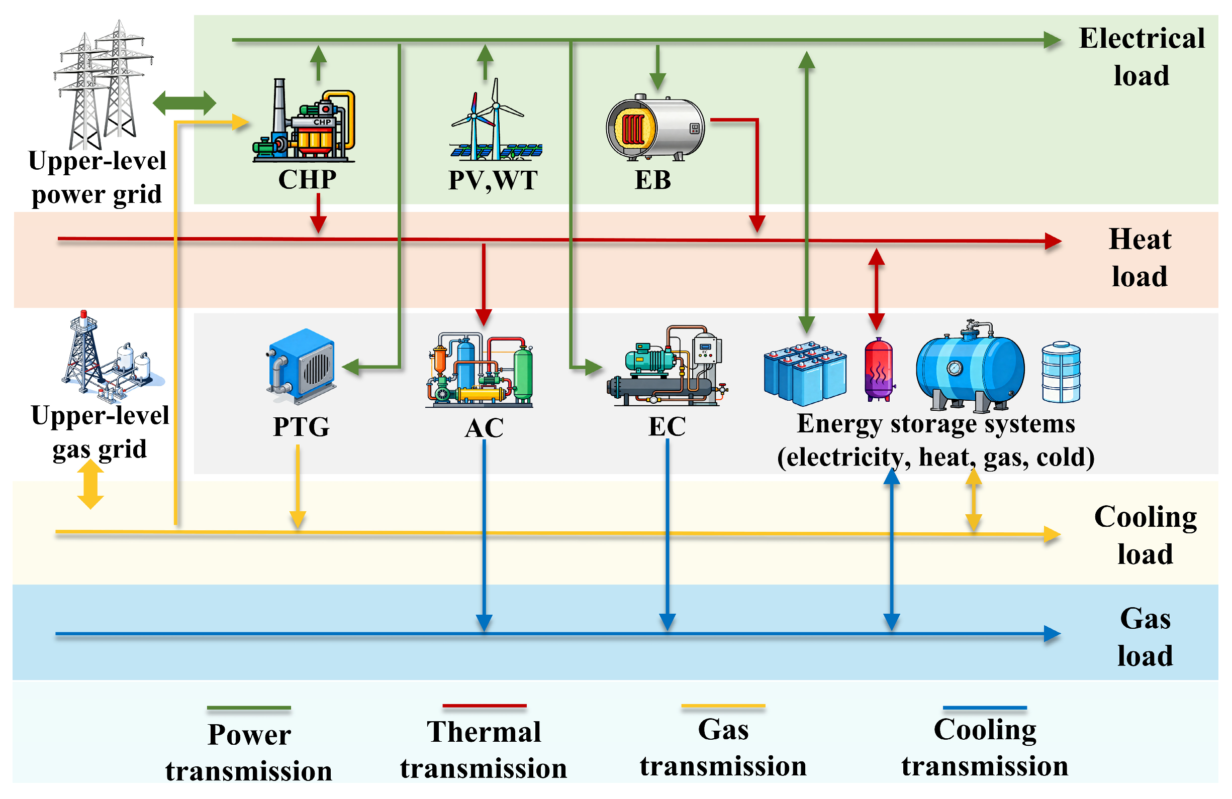
1. Introduction

Carbon-neutrality targets are accelerating the development of cleaner and more tightly coupled integrated energy systems (IESs). By coordinating electricity, heat, gas, and cooling, an IES can accommodate renewable generation and make better use of conversion and storage assets. Low emissions alone, however, do not guarantee operational sustainability. A practical schedule must also be economical, measurable, and compatible with users’ energy-service needs. Three gaps remain. First, carbon management is usually planned over medium- or long-term periods, whereas dispatch decisions are made hourly; seasonal carbon information is therefore difficult to carry into day-ahead operation. Second, conventional price-elastic demand response models do not adequately describe the nonlinear relationship between cooling demand and thermal comfort. Third, the trade-off between operating cost and carbon emissions must be selected transparently, because empirically assigned weights weaken reproducibility. These gaps motivate a framework that connects seasonal carbon planning, comfort-aware demand response, reproducible compromise selection, and hourly multi-energy dispatch.

Demand-side flexibility has become central to the low-carbon operation of IESs as energy carriers become more strongly coupled and carbon-trading mechanisms are introduced. Carbon–energy collaborative dispatch can coordinate energy consumption, emissions, and user response [1]. Previous studies have combined energy certificates, carbon markets, and energy sharing in multi-microgrid, multi-regional, and industrial-park systems, reporting improved renewable-energy accommodation and environmental performance [2,3,4]. Related work has examined coordinated operation under coupled carbon and green-certificate markets [5,6] and has incorporated diversified hydrogen use into multi-timescale optimization [7]. These studies establish the value of market coordination, but seasonal carbon allocation, demand response, thermal comfort, seasonal storage, and multi-objective decision-making are generally treated in separate models. A unified hourly framework is still needed to show how seasonal carbon information becomes a price signal, how cooling flexibility remains within comfort limits, and how the economic–environmental compromise can be reproduced.

A key challenge is how to use coordinated carbon–energy market signals to support the low-carbon operation of multi-energy IESs. Incentive-oriented power–carbon–green certificate markets, CCUS–P2G coupling, hydrogen-blended gas systems, and seasonal carbon trading mechanisms have been explored, showing that incentive design, hydrogen utilization, and temporal carbon allocation can reduce system cost and emissions [8,9,10]. Nash-bargaining pricing, electricity-pricing mechanisms, cross-regional competition, and energy sharing under carbon–green certificate coupling have also been studied, confirming the value of coordinated market interaction [11,12,13,14]. Most of these mechanisms, however, focus on short-term regulation and give limited attention to the transmission of medium- and long-term carbon management information into hourly operation, which restricts coordinated energy and carbon management in IESs.

A further issue is the reproducible selection of an economic–environmental compromise. Multi-objective low-carbon optimization has been investigated at the system-design and regional-planning levels. Reference [15] conducts a 4E assessment and design optimization of a solar–geothermal integrated energy system, whereas Reference [16] studies long-term regional generation planning under carbon cap-and-trade and renewable portfolio standards. Park-level IES clusters, multi-energy collaborative operation, and regional generation-mix optimization have also been considered [17,18,19]. Seasonal carbon-management studies follow different routes: Reference [20] combines carbon mineralization with seasonal energy storage in system planning, while Reference [21] incorporates CCUS and multi-timescale allowance allocation into low-carbon dispatch. These contributions are valuable, but they operate at decision levels that differ from hourly seasonal dispatch. Because objective weights are still often chosen empirically, a transparent compromise-selection procedure is needed to make the trade-off easier to reproduce and interpret.

This study addresses the above gaps through a multi-timescale low-carbon economic scheduling framework for a multi-energy IES. First, historical renewable-generation and load data are used to derive seasonal carbon-pressure signals, and carbon allowances are mapped to hourly accounting intervals. Medium- and long-term carbon information can therefore influence short-term dispatch without changing the one-hour resolution. Second, carbon-trading incentive and disincentive signals are embedded in electricity, heat, and gas prices, while cooling demand is modeled separately with a fuzzy thermal-comfort mechanism. Representative wind and photovoltaic profiles are constructed through sampling and scenario reduction. Third, a nested IGA–CPLEX procedure separates compromise-weight search from constrained hourly dispatch: CPLEX solves the mixed-integer model for each candidate economic weight, and the outer IGA evaluates the normalized economic–environmental result. The IGA is used as an extensible search mechanism, not as proof of a unique preference or universal superiority, and its result is checked against deterministic and population-based alternatives. Multiple storage devices, including seasonal gas storage, are coordinated across the four representative seasonal profiles. The resulting model jointly minimizes operating cost and physical carbon emissions while linking seasonal carbon planning, comfort-aware demand response, compromise selection, and hourly multi-energy operation.

From an operational-sustainability perspective, the framework links four dimensions that are commonly assessed in isolation. The environmental dimension is represented by physical-emission accounting and the coordinated use of renewable generation, conversion units, storage, and flexible demand. Economic feasibility is represented by operating cost and the normalized cost–emission compromise. User acceptability is retained through PMV-constrained cooling response, so flexibility is obtained without removing explicit comfort limits. Finally, the seasonal carbon-pressure indicator and hourly carbon accounting provide measurable signals that a park-level energy manager or aggregator can update and monitor. Put simply, the method is an operational decision-support tool rather than a complete social or life-cycle sustainability assessment; it converts carbon-management information into day-ahead actions within a clearly defined model boundary.

The study therefore focuses on one specific transmission path: historical seasonal carbon-pressure information is converted into carbon-embedded electricity, heat, and gas prices, and these signals are coordinated with comfort-aware cooling response, seasonal gas storage, and compromise-weight selection in a unified hourly model. The method does not replace carbon-market settlement or reproduce annual allowance allocation. Its purpose is to bring seasonal carbon information into short-term multi-energy operating decisions.

Table 1. Comparison with recent low-carbon scheduling approaches.

Approach	Main Mechanism	Main Emphasis	Difference from the Present Study
Carbon and certificate trading	Carbon market, renewable certificates, and energy sharing	Multi-market participation and avoidance of overlapping benefits	Does not introduce a historical seasonal carbon-pressure signal into multi-energy demand response
Seasonal carbon trading	Seasonal carbon trading, hydrogen storage, and quota sharing	Seasonal hydrogen utilization and multi-agent energy sharing	Focuses on hydrogen and quota exchange rather than comfort-aware electricity–heat–gas–cooling response
Multi-timescale allowance allocation	Annual allowance allocation and short-term dispatch	Consistency between annual compliance and operational scheduling	Uses an annual model, whereas the present study is limited to four representative seasonal days
Ladder-type carbon trading	CCUS–P2G coupling and reward–penalty carbon pricing	Detailed low-carbon technology coupling and carbon-price sensitivity	Uses a technology-oriented ladder price rather than data-derived seasonal carbon-pressure factors
Present study	Seasonal carbon-embedded prices, demand response, SGS, and compromise weight selection	Transmission of seasonal carbon information to hourly multi-energy dispatch	Integrates seasonal signals with differentiated demand response and representative-horizon scheduling

positions the framework relative to recent low-carbon scheduling approaches.

Relationship to our previous work. The park-level electricity–heat–gas–cooling–carbon configuration, carbon–energy pricing mechanism, seasonal carbon-planning framework, baseline electricity–heat–gas demand-response model, and general seasonal-storage concept are inherited from our previous study [22]. They serve as the baseline formulation and are not presented here as new contributions.

The present paper adds two methodological extensions to Reference [22]. First, cooling demand is separated from the price-elastic electricity, heat, and gas loads and represented by an independent piecewise response linked to fuzzy thermal-comfort information. Section 3.2.3 develops this formulation to reflect the distinct thermal characteristics of cooling demand. Second, Section 4.2 and Section 4.3 introduce a normalized economic–environmental compromise-selection procedure. The outer IGA searches the economic preference weight, the inner CPLEX model solves the corresponding mixed-integer hourly dispatch problem, and the preferred solution is chosen by its normalized distance from the economic–environmental ideal point.

In addition to these methodological extensions, the numerical analysis examines their interaction with the inherited seasonal carbon pricing and seasonal gas storage mechanisms.

2. System Configuration and Baseline Operational Model

The baseline park-level electricity–heat–gas–cooling system and its principal energy-conversion, storage, and balance relationships are adapted from our previous work [22] and are restated here to keep the present formulation self-contained. The new formulations developed in this paper are concentrated in Section 3.2.3, which presents the differentiated cooling load response model, and Section 4.2 and Section 4.3, which present the normalized compromise-selection and IGA–CPLEX solution procedure.

This section gives a compact description of the baseline system and the constraints needed for the subsequent scheduling model. The inherited seasonal carbon pricing, representative-profile, and storage formulations are retained as supporting components. The methodological extensions claimed in this paper are limited to the differentiated cooling load response in Section 3.2.3 and the normalized compromise-selection procedure in Section 4.2 and Section 4.3.

2.1. Multi-Energy Integrated System Framework

The studied IES contains renewable generation units, energy-conversion units, energy storage devices, multi-energy loads, and interfaces with the external electricity and gas networks. Wind turbines and photovoltaic units supply renewable electricity. The conversion layer includes a combined heat and power unit, an electric boiler, a power-to-gas unit, an electric chiller, and an absorption chiller. Electrical, thermal, gas, cooling, and seasonal gas storage devices are coordinated to support both short-term energy balancing and inter-segment gas inventory coordination across the four representative seasonal profiles. This results in a highly integrated, multi-energy complementary system, as depicted in Figure 1. The classification and full names of the functional entities are presented in

Table 2. Classification of IES entities.

Category	Main Entities	Abbreviation
Energy production	Wind turbine	WT
	Photovoltaic	PV
Energy storage	Storage battery unit	SBU
	Gas storage tank	GST
	Heat storage tank	HST
	Ice storage tank	IST
	Seasonal gas storage tank	SGS
Energy conversion	Combined heat and power unit	CHP
	Electric boiler	EB
	Power to gas	P2G
	Electric chiller	EC
	Absorption chiller	AC
External interface	Power grid	—
	Gas grid	—
End-user load	Electrical load	—
	Heat load	—
	Cooling load	—
	Gas load	—

.

2.2. Carbon Emission and Energy Allocation Modeling

2.2.1. Energy Production

To address the timescale mismatch between carbon trading and energy dispatch, this paper maps carbon allowances and actual carbon emissions to the one-hour scheduling intervals adopted in the energy dispatch model. Carbon allowances are allocated according to the carbon allowance allocation benchmark and the corresponding energy output or consumption, while actual carbon emissions are calculated using carbon emission coefficients. This discretization is an operational timescale mapping rather than a change in the actual carbon market settlement period. Since the cumulative carbon allowances and cumulative carbon emissions over the whole scheduling horizon remain unchanged, this treatment does not introduce systematic errors in the total carbon balance [22].

The seasonal optimal scheduling framework refers to the incorporation of seasonal carbon emission characteristics and low-carbon demand signals into the hourly dispatch process, rather than a seasonal-scale dispatch interval. Therefore, the proposed method integrates seasonal-level carbon planning with hourly operational scheduling.

WT and PV convert wind and solar energy into electricity without direct operating emissions. The allowances assigned to these units are therefore not compensation for their own emissions; they represent an incentive based on the fossil-fuel emissions avoided by renewable generation under the adopted benchmark method. The carbon allowance model for WT and PV in an IES is expressed as

$$\left\{\begin{array}{l}{A}_{\mathrm{WT}}=B_{\mathrm{res}}^{\mathrm{WT}}{P}_{\mathrm{WT}}\\ A_{\mathrm{PV}}=B_{\mathrm{res}}^{\mathrm{PV}}{P}_{\mathrm{PV}}\end{array}\right.$$

(1)

where $A_{\mathrm{W}\mathrm{T}}$ and $A_{\mathrm{P}\mathrm{V}}$ are the allocated carbon allowances for WT and PV, respectively; $B_{\mathrm{r}\mathrm{e}\mathrm{s}}^{\mathrm{W}\mathrm{T}}$ and $B_{\mathrm{r}\mathrm{e}\mathrm{s}}^{\mathrm{P}\mathrm{V}}$ are the allocation benchmark values for the power supply carbon allowances for WT and PV, respectively; $P_{\mathrm{W}\mathrm{T}}$ and $P_{\mathrm{P}\mathrm{V}}$ are the output power of WT and PV, respectively.

2.2.2. Energy Conversion

Energy conversion units provide the main coupling paths among the energy carriers. Their operating relationships and carbon allowance formulations are given below.

(1)

CHP mathematical model

$$\left\{\begin{array}{l}{P}_{\mathrm{CHP}}={\eta }_{\mathrm{CHP}}^{\mathrm{p}}{G}_{\mathrm{CHP}}\\ H_{\mathrm{CHP}}={\eta }_{\mathrm{CHP}}^{\mathrm{h}}{P}_{\mathrm{CHP}}{F}_{\mathrm{r}}\\ D_{\mathrm{CHP}}={\lambda }_{\mathrm{CHP}}^{\mathrm{g}}{G}_{\mathrm{CHP}}\\ A_{\mathrm{CHP}}=P_{\mathrm{CHP}}{B}_{\mathrm{CHP}}^{\mathrm{p}}+H_{\mathrm{CHP}}{B}_{\mathrm{CHP}}^{\mathrm{h}}\end{array}\right.$$

(2)

where PCHP is the electrical output of the CHP unit; HCHP is its thermal output; GCHP is its gas input; ηCHPp and ηCHPh are the electrical and thermal conversion efficiencies, respectively; DCHP is the direct carbon emission from CHP fuel use; λCHPg is the gas-combustion carbon emission coefficient; ACHP is the carbon allowance allocated to CHP; BCHPp and BCHPh are the electricity- and heat-supply allowance benchmarks, respectively; and Fr is the CHP heat-supply correction coefficient.

(2)

EB mathematical model

$$\left\{\begin{array}{l}{H}_{\mathrm{EB}}={\eta }_{\mathrm{EB}}{P}_{\mathrm{EB}}\\ A_{\mathrm{EB}}=B_{\mathrm{EB}}^{\mathrm{p}}{P}_{\mathrm{EB}}\end{array}\right.$$

(3)

where HEB is the thermal output of EB; ηEB is its conversion efficiency; PEB is its electrical input; AEB is the carbon allowance allocated to EB; and BEBp is the benchmark for heat-supply allowance allocation.

(3)

P2G mathematical model

$$\left\{\begin{array}{l}{G}_{\mathrm{P}2\mathrm{G}}={\eta }_{\mathrm{P}2\mathrm{G}}{P}_{\mathrm{P}2\mathrm{G}}\\ D_{\mathrm{P}2\mathrm{G}}={\lambda }_{\mathrm{P}2\mathrm{G}}^{\mathrm{g}}{G}_{\mathrm{P}2\mathrm{G}}\\ A_{\mathrm{P}2\mathrm{G}}=B_{\mathrm{P}2\mathrm{G}}^{\mathrm{g}}{G}_{\mathrm{P}2\mathrm{G}}\end{array}\right.$$

(4)

where GP2G is the gas output of P2G; ηP2G is its conversion efficiency; PP2G is the electrical input of P2G; DP2G is the carbon-consumption quantity associated with gas production; λP2Gg is the carbon-consumption coefficient, taken with the sign convention used in the carbon balance; AP2G is the carbon allowance allocated to P2G; and BP2Gp is the gas-supply allowance benchmark.

(4)

EC mathematical model

$$\left\{\begin{array}{l}{L}_{\mathrm{EC}}=m_{\mathrm{EC}}{P}_{\mathrm{EC}}\\ A_{\mathrm{EC}}=B_{\mathrm{EC}}{P}_{\mathrm{EC}}\end{array}\right.$$

(5)

where LEC is the cooling output of EC; mEC is its coefficient of performance; PEC is its electrical input; AEC is the carbon allowance allocated to EC; and BEC is the electricity-supply allowance benchmark.

(5)

AC mathematical model

$$\left\{\begin{array}{l}{L}_{\mathrm{AC}}=m_{\mathrm{AC}}{H}_{\mathrm{AC}}\\ A_{\mathrm{AC}}=B_{\mathrm{AC}}{H}_{\mathrm{AC}}\\ D_{\mathrm{AC}}={\lambda }_{\mathrm{AC}}{H}_{\mathrm{AC}}\end{array}\right.$$

(6)

where LAC is the cooling output of AC; mAC is its coefficient of performance; HAC is its thermal input; AAC is the carbon allowance allocated to AC; and BAC is the heat-supply allowance benchmark. DAC denotes the carbon quantity attributed to the heat input of AC for internal carbon accounting; it is not counted again as an independent source in the physical emission objective.

2.2.3. Energy Storage

$$S_{\mathrm{SBU}}(t+1)=S_{\mathrm{SBU}}(t)-S_{\mathrm{SBU}}^{\mathrm{loss}}(t)+{\displaystyle \frac{{\eta }_{\mathrm{c}}^{\mathrm{SBU}}{P}_{\mathrm{c}}^{\mathrm{SBU}}(t)-P_{\mathrm{d}}^{\mathrm{SBU}}(t)/{\eta }_{\mathrm{d}}^{\mathrm{SBU}}}{E_{\mathrm{SBU}}}}$$

(7)

$$\left\{\begin{array}{l}0\le S_{\mathrm{SBU}}(t)\le 1\\ P_{\mathrm{c}\min }^{\mathrm{SBU}}\le P_{\mathrm{c}}^{\mathrm{SBU}}(t)\le P_{\mathrm{c}\max }^{\mathrm{SBU}}\\ P_{\mathrm{d}\min }^{\mathrm{SBU}}\le P_{\mathrm{d}}^{\mathrm{SBU}}(t)\le P_{\mathrm{d}\max }^{\mathrm{SBU}}\\ 0\le h_{\mathrm{c}}^{\mathrm{SBU}}+h_{\mathrm{d}}^{\mathrm{SBU}}\le 1\end{array}\right.$$

(8)

where SSBU(t) is the state of charge of the SBU at time t; SSBUloss(t) is its self-loss; ηcSBU and ηdSBU are the charging and discharging efficiencies; ESBU is the maximum energy capacity; Pc,maxSBU and Pd,maxSBU are the maximum charging and discharging powers; Pc,minSBU and Pd,minSBU are the corresponding minimum powers; and hcSBU and hdSBU are binary charging and discharging indicators. GST, SGS, HST, and IST use the same state-transition structure, with device-specific capacities, efficiencies, and energy carriers.

2.2.4. External Network Interfaces

$$\left\{\begin{array}{l}-P_{\mathrm{GRID}}^{\mathrm{tran},\max }\le P_{\mathrm{GRID}}^{\mathrm{tran}}\le P_{\mathrm{GRID}}^{\mathrm{tran},\max }\\ -G_{\mathrm{NET}}^{\mathrm{tran},\max }\le G_{\mathrm{NET}}^{\mathrm{tran}}\le G_{\mathrm{NET}}^{\mathrm{tran},\max }\end{array}\right.$$

(9)

$$\left\{\begin{array}{l}{D}_{\mathrm{GRID}}={\lambda }_{\mathrm{GRID}}^{\mathrm{p}}{P}_{\mathrm{GRID}}^{\mathrm{tran}}\\ {\lambda }_{\mathrm{GRID}}^{\mathrm{p}}={\lambda }_{\mathrm{GRID}}^{\mathrm{gas}}{\alpha }_{\mathrm{gas}}+{\lambda }_{\mathrm{GRID}}^{\mathrm{coal}}{\alpha }_{\mathrm{coal}}\end{array}\right.$$

(10)

where PGRIDtran and GNETtran are the electrical and gas powers exchanged with the external power and gas grids, respectively; PGRIDtran,max and GNETtran,max are the corresponding exchange limits; DGRID is the upstream carbon emission associated with purchased electricity; λGRIDp is the grid electricity carbon emission coefficient; λGRIDgas and λGRIDcoal are the gas- and coal-fired generation emission coefficients used to construct λGRIDp; and αgas and αcoal are their shares in the regional generation mix. The external grids are represented as capacity-limited interfaces rather than detailed network models.

2.2.5. System-Wide Dynamic Balance Model

$$\left\{\begin{array}{l}{P}_{\mathrm{WT}}+P_{\mathrm{PV}}+P_{\mathrm{CHP}}\pm P_{\mathrm{SBU}}\pm P_{\mathrm{GRID}}^{\mathrm{tran}}=P_{\mathrm{EB}}+P_{\mathrm{P}2\mathrm{G}}+P_{\mathrm{EC}}+P_{\mathrm{load}}\\ H_{\mathrm{CHP}}+H_{\mathrm{EB}}\pm H_{\mathrm{HST}}=H_{\mathrm{AC}}+H_{\mathrm{load}}\\ G_{\mathrm{PTG}}\pm G_{\mathrm{GST}}\pm G_{\mathrm{SGS}}\pm G_{\mathrm{NET}}^{\mathrm{tran}}=G_{\mathrm{CHP}}+G_{\mathrm{load}}\\ L_{\mathrm{EC}}+L_{\mathrm{AC}}\pm L_{\mathrm{IST}}=L_{\mathrm{load}}\\ D_{\mathrm{CHP}}+D_{\mathrm{GRID}}-D_{\mathrm{PTG}}=A_{\mathrm{WT} }+A_{\mathrm{PV}}+A_{\mathrm{CHP}}+A_{\mathrm{EB}}+A_{\mathrm{AC}}+A_{\mathrm{PTG}}\pm A_{\mathrm{tran}}\end{array}\right.$$

(11)

where Pload, Hload, Gload, and Lload are the electricity, heat, gas, and cooling demands, respectively; and Atran is the net carbon allowance exchanged with the external carbon market.

3. Low-Carbon Energy Demand Response Strategy Based on a Carbon–Energy Trading Market

This section develops a seasonally differentiated demand response mechanism for the studied IES. The purpose of this mechanism is to transmit the environmental cost of energy consumption to the user side through price signals, thereby coordinating multi-energy demand adjustment with the system-level carbon-reduction objective.

In the considered park-level or regional IES, the energy management center or energy aggregator acts as the market participant. It conducts energy and carbon transactions on behalf of the users and converts the carbon trading information into electricity, gas, and heat price signals. Therefore, end users do not directly participate in carbon allowance settlement; instead, they adjust their consumption patterns in response to carbon-embedded energy prices. The users are assumed to be located within the same region and to experience similar seasonal and climatic conditions, which allows the demand response strategy to be implemented in a coordinated manner.

The hourly representation is introduced to maintain a consistent temporal resolution between carbon accounting and energy dispatch. It does not reproduce or modify the settlement period of the actual carbon market. In this study, cumulative carbon allowances and physical emissions refer only to the modeled representative-day horizon and should not be interpreted as annual settlement quantities.

3.1. A Carbon–Energy Trading Market

The carbon–energy trading market is modeled as a coordinated mechanism linking energy conversion, external exchange, end-use demand, storage operation, and carbon accounting. By embedding carbon trading information in energy prices, the model addresses the mismatch between allocated allowances and operating emissions without changing the underlying carbon market settlement period.

Within this carbon–energy trading market, the various resource interaction prices among the IES entities are unified into a carbon–energy price. By introducing a carbon price adjustment coefficient, the carbon trading incentive–disincentive price mechanism is embedded in energy pricing, thereby laying the foundation for the subsequent integration of seasonal carbon-pressure factors. The detailed calculation process is outlined as follows.

$$\left\{\begin{array}{l}{c}_{\mathrm{ele}}^{\mathrm{car}}(t)=c_{\mathrm{ele}}(t)+{\phi }_{\mathrm{e}}^{\mathrm{car}}{c}_{\mathrm{car}}(t)\\ c_{\mathrm{gas}}^{\mathrm{car}}(t)=c_{\mathrm{gas}}(t)+{\phi }_{\mathrm{g}}^{\mathrm{car}}{c}_{\mathrm{car}}(t)\\ c_{\mathrm{heat}}^{\mathrm{car}}(t)=c_{\mathrm{heat}}(t)+{\phi }_{\mathrm{h}}^{\mathrm{car}}{c}_{\mathrm{car}}(t)\end{array}\right.$$

(12)

where $c_{\mathrm{e}\mathrm{l}\mathrm{e}}^{\mathrm{c}\mathrm{a}\mathrm{r}}(t)$, $c_{\mathrm{g}\mathrm{a}\mathrm{s}}^{\mathrm{c}\mathrm{a}\mathrm{r}}(t)$, and $c_{\mathrm{h}\mathrm{e}\mathrm{a}\mathrm{t}}^{\mathrm{c}\mathrm{a}\mathrm{r}}(t)$ are the carbon-embedded electricity, gas, and heat prices, respectively. The corresponding conventional energy prices are denoted by $c_{\mathrm{e}\mathrm{l}\mathrm{e}}(t)$, $c_{\mathrm{g}\mathrm{a}\mathrm{s}}(t)$, and $c_{\mathrm{h}\mathrm{e}\mathrm{a}\mathrm{t}}(t)$. $c_{\mathrm{c}\mathrm{a}\mathrm{r}}(t)$ represents the carbon trading incentive–disincentive price, while ${\phi }_{\mathrm{e}}^{\mathrm{c}\mathrm{a}\mathrm{r}}$, ${\phi }_{\mathrm{g}}^{\mathrm{c}\mathrm{a}\mathrm{r}}$, and ${\phi }_{\mathrm{h}}^{\mathrm{c}\mathrm{a}\mathrm{r}}$ are the conversion coefficients used to allocate the carbon-price signal to the three energy carriers. These coefficients reflect the carbon emission characteristics of the corresponding energy-supply processes.

3.2. Low-Carbon Energy Demand Response Strategy

The low-carbon demand-response strategy connects carbon-management information with multi-energy load adjustment across two timescales. Historical data are used first to estimate seasonal carbon-pressure signals. Those signals are then embedded in carbon–energy prices that guide the hourly response of users.

The coupling is sequential. Historical renewable-generation and multi-energy load data are processed to obtain one carbon-pressure factor for each season. The factors are not re-optimized in the hourly dispatch model; they enter as fixed parameters for the spring, summer, autumn, and winter representative segments.

During each hourly interval, the relevant seasonal factor adjusts the carbon-embedded electricity, heat, and gas prices. The demand-response model uses these prices to determine the curtailable and shiftable portions of the loads, after which the revised profiles enter the energy-balance, equipment-operation, storage-state, and carbon-accounting constraints. In this way, medium- and long-term information reaches hourly operation through a clear price–demand–dispatch chain, while the one-hour scheduling resolution is retained.

3.2.1. Seasonal Carbon Emissions Planning

Based on historical data on clean energy output and load demand in the IES region, the distribution characteristics of these variables across seasons and over extended timescales can be analyzed. Using time series analysis, the seasonal fluctuation component of IES carbon emissions can be extracted. The specific procedure is as follows.

First, to analyze the operational characteristics of the IES, the data for clean energy output and load demand within the region are normalized, and corresponding weighting factors are assigned based on installed capacity. The difference between the load demand and clean energy output is calculated to determine the net load demand.

$$\left\{\begin{array}{l}{\tilde{P}}_{\mathrm{WT}}^{y,m}={\displaystyle \frac{P_{\mathrm{WT}}^{y,m}}{P_{\mathrm{WT}}^{\mathrm{ref}}}},{\tilde{P}}_{\mathrm{PV}}^{y,m}={\displaystyle \frac{P_{\mathrm{PV}}^{y,m}}{P_{\mathrm{PV}}^{\mathrm{ref}}}}\\ {\tilde{L}}_k^{y,m}={\displaystyle \frac{L_k^{y,m}}{L_k^{\mathrm{ref}}}}, k\in [e,h,g,c]\end{array}\right.$$

(13)

$$\left\{\begin{array}{l}{\tilde{P}}_{re}^{y,m}={\omega }_{\mathrm{WT}}{\tilde{P}}_{\mathrm{WT}}^{y,m}+{\omega }_{\mathrm{PV}}{\tilde{P}}_{\mathrm{PV}}^{y,m}\\ {\tilde{L}}_{eq}^{y,m}={\displaystyle \sum _{k\in \{e,h,g,c\}}{\omega }_k}{\tilde{L}}_k^{y,m}\end{array}\right.$$

(14)

$${\tilde{L}}_{\mathrm{net}}^{y,m}={[{\tilde{L}}_{\mathrm{eq}}^{y,m}-{\tilde{P}}_{\mathrm{re}}^{y,m}]}^{+}$$

(15)

where ${\tilde{P}}_{\mathrm{W}\mathrm{T}}^{y,m}$ and ${\tilde{P}}_{\mathrm{P}\mathrm{V}}^{y,\mathrm{m}}$ are the normalized WT and PV outputs, respectively; $P_{\mathrm{W}\mathrm{T}}^{y,\mathrm{m}}$ and $P_{\mathrm{P}\mathrm{V}}^{y,\mathrm{m}}$ are the historical WT and PV outputs, respectively; $P_{\mathrm{W}\mathrm{T}}^{\mathrm{r}\mathrm{e}\mathrm{f}}$, $P_{\mathrm{P}\mathrm{V}}^{\mathrm{r}\mathrm{e}\mathrm{f}}$, and $L_k^{\mathrm{r}\mathrm{e}\mathrm{f}}$ are the corresponding reference values; $L_k^{y,\mathrm{m}}$ is the historical load demand of energy type $k$, including electricity, heat, gas, and cooling; ${\tilde{L}}_k^{y,\mathrm{m}}$ is the normalized load demand;${ \omega }_{\mathrm{W}\mathrm{T}}$ and ${\omega }_{\mathrm{P}\mathrm{V}}$ are the weighting coefficients of WT and PV output, which are determined according to their installed capacities; ${\omega }_k$ is the weighting coefficient of load type $k$, which reflects the relative proportion of different energy loads in the IES; ${\tilde{L}}_{\mathrm{e}\mathrm{q}}^{y,m}$ is the equivalent load demand; ${\tilde{P}}_{\mathrm{e}\mathrm{q}}^{y,m}$ is the equivalent renewable output; ${\tilde{L}}_{\mathrm{n}\mathrm{e}\mathrm{t}}^{y,m}$ is the net load demand.

Next, the carbon emissions associated with the net load are estimated from the operating characteristics of the modeled carbon-emitting sources. Time-series analysis is then used to extract the seasonal component of the resulting carbon indicator.

$$D_{\mathrm{IES}}^{y,m}={\displaystyle \sum _{t\in T_m}{D}_{\mathrm{CHP},t}^y+D_{\mathrm{grid},t}^y+D_{\mathrm{AC},t}^y+D_{\mathrm{PTG},t}^y}$$

(16)

$$D_{\mathrm{IES}}^{y,m}=T^{y,m}+S^{y,m}+{\epsilon }^{y,m}$$

(17)

$$\left\{\begin{array}{l}{D}_{\mathrm{IES},\mathrm{s}}^y={\displaystyle \sum _{m\in {\mathrm{M}}_{\mathrm{s}}}{D}_{\mathrm{IES}}^{y,m}}\\ D_{\mathrm{IES},\mathrm{ann}}^y={\displaystyle \sum _s{D}_{\mathrm{IES},\mathrm{sea}}^y}\end{array}\right.$$

(18)

$$n_s={\displaystyle \frac{1}{Y}}{\displaystyle \sum _{y=1}^Y\frac{D_{\mathrm{IES},s}^y}{D_{\mathrm{IES},\mathrm{ann}}^y}}$$

(19)

where DIESy,m is the monthly carbon indicator used to derive the seasonal pressure signal; Tm is the set of hourly periods in month m; DCHP,ty and DGRID,ty are the direct CHP and purchased electricity emission terms; DAC,ty is the carbon quantity attributed to AC heat input for the historical indicator; and DP2G,ty is the P2G carbon-consumption term under the sign convention of the system carbon balance Equation (11). Ty,m, Sy,m, and εy,m are the trend, seasonal, and residual components, respectively; DIES,sy is the seasonal carbon indicator; DIES,anny is the annual total of that indicator; Y is the number of historical years; and ns is the seasonal carbon-pressure signal. This historical indicator is used only to construct seasonal price signals and is distinct from the physical emission objective in Section 4.1.

The seasonal component is used to construct one carbon-pressure coefficient for each season, and the corresponding carbon–energy prices are adjusted accordingly. This step transmits the historical seasonal pattern to the demand response model; it is not an annual allowance settlement calculation.

$$\left\{\begin{array}{l}{c}_{\mathrm{ele}}^{\mathrm{car}}(t)=c_{\mathrm{ele}}(t)+n_{\mathrm{car}}^{\mathrm{sea}}{\psi }_{\mathrm{e}}^{\mathrm{car}}{c}_{\mathrm{car}}(t)\\ c_{\mathrm{gas}}^{\mathrm{car}}(t)=c_{\mathrm{gas}}(t)+n_{\mathrm{car}}^{\mathrm{sea}}{\psi }_{\mathrm{g}}^{\mathrm{car}}{c}_{\mathrm{car}}(t)\\ c_{\mathrm{heat}}^{\mathrm{car}}(t)=c_{\mathrm{heat}}(t)+n_{\mathrm{car}}^{\mathrm{sea}}{\psi }_{\mathrm{h}}^{\mathrm{car}}{c}_{\mathrm{car}}(t)\end{array}\right.$$

(20)

where ncar,sprsea, ncar,sumsea, ncar,autsea, and ncar,winsea are the carbon-pressure signals for spring, summer, autumn, and winter, respectively. To reduce year-specific noise, each seasonal signal is calculated from the multi-year average of the corresponding seasonal component.

3.2.2. Low-Carbon Energy Demand Response

To characterize the response of electric demand to time-varying electricity prices, a matrix-based price elasticity model is adopted. Let

$$T=\{1,2,\dots ,T\}$$

(21)

denote the set of scheduling intervals. The baseline electricity price and the adjusted electricity price in interval $j$ are represented by $c_{\mathrm{e}}^0\left(j\right)$ and $c_{\mathrm{e}}\left(j\right)$, respectively. The normalized electricity-price deviation is defined as

$${\delta }_{\mathrm{e}}(j)={\displaystyle \frac{c_{\mathrm{e}}(j)-c_{\mathrm{e}}^0(j)}{c_{\mathrm{e}}^0(j)}},\hspace{1em}j\in T$$

(22)

The baseline electric demand is divided into conventional demand, curtailable demand, and shiftable demand. The portions of the baseline load that participate in load curtailment and load shifting are determined by the corresponding participation ratios. The resulting demand response model is formulated as

$$\left\{\begin{array}{l}{P}_{\mathrm{CL}}^0(t)={\alpha }_{\mathrm{cut}}{P}_{\mathrm{L}}^0(t)\\ P_{\mathrm{SL}}^0(t)={\alpha }_{\mathrm{shift}}{P}_{\mathrm{L}}^0(t)\\ \Delta P_{\mathrm{CL}}(t)=P_{\mathrm{CL}}^0(t){\displaystyle \sum _{j\in T}{e}_{\mathrm{CL}}(t,j){\delta }_e(j)}\\ \Delta P_{\mathrm{SL}}(t)=P_{\mathrm{SL}}^0(t){\displaystyle \sum _{j\in T}{e}_{\mathrm{SL}}(t,j){\delta }_e(j)}\\ P_{\mathrm{L}}^{\mathrm{DR}}(t)=P_{\mathrm{L}}^0(t)+\Delta P_{\mathrm{CL}}(t)+\Delta P_{\mathrm{SL}}(t)\\ t\in T\end{array}\right.$$

(23)

Here, $\Delta P_{\mathrm{C}\mathrm{L}}\left(t\right)$ and $\Delta P_{\mathrm{S}\mathrm{L}}\left(t\right)$ are defined as signed load variations. Specifically, a negative value of $\Delta P_{\mathrm{C}\mathrm{L}}\left(t\right)$ indicates that part of the electric demand is curtailed. For the shiftable load, a positive value of $\Delta P_{\mathrm{S}\mathrm{L}}\left(t\right)$ means that load is shifted into interval $t$, whereas a negative value means that load is shifted out of that interval. The transferable-load response is restricted to predefined hourly periods within the same representative day. Elements of the transfer elasticity matrix that connect different seasonal profiles or fall outside the allowable response window are set to zero.

The elements of the price elasticity matrices are defined as

$$e_k(t,j)={\left.{\displaystyle \frac{\partial P_k(t)}{\partial c_{\mathrm{e}}(j)}}\right|}_{\left(P_k^0,c_{\mathrm{e}}^0\right)}{\displaystyle \frac{c_{\mathrm{e}}^0(j)}{P_k^0(t)}}\approx {\displaystyle \frac{\Delta P_k(t)/P_k^0(t)}{\left[c_{\mathrm{e}}(j)-c_{\mathrm{e}}^0(j)\right]/c_{\mathrm{e}}^0(j)}},\hspace{1em}k\in \{\mathrm{CL},\mathrm{SL}\}$$

(24)

where ektj denotes the sensitivity of demand type k in interval t to the price variation in interval j. The diagonal elements ektt represent self-price elasticity, whereas the off-diagonal elements ektj (t ≠ j) describe intertemporal load transfer. The load-reduction elasticity matrix represents curtailable demand and is diagonal, with entries of −0.12, −0.10, and −0.08 for electricity, heat, and gas, respectively. The load-transfer matrices have diagonal entries of −0.10, −0.08, and −0.06. Positive cross-price elasticities are distributed among the permitted destination periods according to temporal distance, and each row sums to zero so that shiftable-load energy is conserved.

For curtailable loads, self-price elasticity is negative because a higher price reduces demand in the same interval. For shiftable loads, the diagonal elements are negative and selected off-diagonal elements are positive, representing demand moved from higher-price intervals to permitted lower-price intervals within the same representative day.

The procedure is straightforward: historical data provide the seasonal carbon-pressure information, and the carbon–energy prices carry that information into the hourly demand response calculation. The resulting load profiles are then passed to the dispatch model. This sequence links medium-term carbon information with short-term operation without implying that end-use demand is transferred between seasons.

3.2.3. Cooling Load Demand Response with Fuzzy Thermal Comfort

Cooling demand differs from electricity, heat, and gas demand because its adjustment directly affects the indoor thermal environment. Therefore, cooling load flexibility is modeled by combining building thermal dynamics with a thermal comfort constraint [23].

$$T_{s,t+1}^{\mathrm{in}}=T_{s,t}^{\mathrm{in}}+{\displaystyle \frac{\Delta t}{C_{\mathrm{b}}}}\left[{\displaystyle \frac{T_{s,t}^{\mathrm{out}}-T_{s,t}^{\mathrm{in}}}{R_{\mathrm{b}}}}+Q_{s,t}^{\mathrm{int}}+Q_{s,t}^{\mathrm{sol}}-L_{s,t}^{\mathrm{cool}}\right]$$

(25)

where $T_{s,t}^{\mathrm{i}\mathrm{n}}$ and $T_{s,t}^{\mathrm{o}\mathrm{u}\mathrm{t}}$ are the indoor and outdoor temperatures, respectively; $R_{\mathrm{b}}$ and $C_{\mathrm{b}}$ are the equivalent thermal resistance and thermal capacitance of the building; $Q_{s,t}^{\mathrm{i}\mathrm{n}\mathrm{t}}$ and $Q_{s,t}^{\mathrm{s}\mathrm{o}\mathrm{l}}$ represent internal and solar heat gains; and $L_{s,t}^{\mathrm{c}\mathrm{o}\mathrm{o}\mathrm{l}}$ is the cooling load after demand response.

Occupants’ thermal comfort is evaluated using the Predicted Mean Vote index. PMV is calculated from the indoor air temperature, mean radiant temperature, relative humidity, indoor air velocity, clothing insulation, and metabolic rate:

$${\mathrm{PMV}}_{s,t}=F_{\mathrm{PMV}}\left(T_{s,t}^{\mathrm{in}},T_{s,t}^{\mathrm{r}},R{H}_{s,t},v_{s,t},I_{\mathrm{cl},s,t},M_{s,t}\right)$$

(26)

The PMV calculation follows the thermal comfort formulation cited in [23]. To maintain compatibility with the mixed-integer linear dispatch model, the nonlinear PMV–temperature relationship is evaluated offline under the adopted environmental and occupant parameters and represented by a piecewise-linear approximation. The comfort constraints should therefore be interpreted under these fixed parameter assumptions.

During occupied periods, the PMV value is constrained within the acceptable comfort interval:

$${\mathrm{PMV}}^{\min }\le {\mathrm{PMV}}_{s,t}\le {\mathrm{PMV}}^{\max }$$

(27)

The cooling load is also limited within an allowable response range relative to the baseline cooling demand:

$$\left(1-{\delta }^{-}\right)L_{s,t}^{\mathrm{cool},0}\le L_{s,t}^{\mathrm{cool}}\le \left(1+{\delta }^{+}\right)L_{s,t}^{\mathrm{cool},0}$$

(28)

The optimization can use building thermal inertia to reshape the hourly cooling profile, but any adjustment must satisfy the indoor temperature and comfort constraints. A terminal indoor temperature condition is imposed for each representative day to avoid an artificial reduction in cooling demand near the end of the horizon. The admissible PMV interval is [−1, 1], with −0.5 and 0.5 used as the internal breakpoints of the piecewise approximation. Indoor temperature is constrained to 24–28 °C, and the cooling load adjustment is limited to ±10% of the baseline load.

4. Seasonal Low-Carbon Economic Dispatch with IGA-Assisted Compromise Weight Selection

The seasonal low-carbon economic dispatch model has a nested structure. For any specified economic–environmental weight pair, the inner model determines the hourly IES schedule. The outer improved genetic algorithm (IGA) searches the admissible economic weight and evaluates the normalized compromise produced by the inner solution. This arrangement reduces dependence on an arbitrarily assigned weight, although it does not identify a unique stakeholder preference.

4.1. Economic and Carbon Emission Objectives

The economic objective considers the operating costs of the energy conversion units, the energy transaction costs with the external power- and gas-grid interfaces, and the operation and maintenance costs of the storage devices. The total operating cost is expressed as

$$F_{\mathrm{eco}}=C_{\mathrm{con}}+C_{\mathrm{net}}+C_{\mathrm{sto}}$$

(29)

The operating cost of the energy-conversion units is calculated as

$$C_{\mathrm{con}}={\displaystyle \sum _{t\in T}{\displaystyle \sum _{i\in I_{\mathrm{con}}}\left[c_i^P{P}_i(t)+c_i^H{H}_i(t)+c_i^G{G}_i(t)+c_i^L{L}_i(t)\right]}}$$

(30)

where $T$ denotes the set of scheduling periods and $I_{\mathrm{c}\mathrm{o}\mathrm{n}}$ denotes the set of energy conversion units. $P_i(t)$, $H_i(t)$, $G_i(t)$, and $L_i(t)$ are the electrical, thermal, gas, and cooling outputs of unit $i$, respectively. The corresponding unit operating cost coefficients are denoted by $c_i^p$, $c_i^g$, $c_i^h$, and $c_i^l$. For a unit that does not produce a particular form of energy, the corresponding term is set to zero.

The transaction cost associated with the external power and gas interfaces is expressed as

$$C_{\mathrm{net}}={\displaystyle \sum _{t\in \mathcal{T}}\left[c_{\mathrm{ele}}^{\mathrm{car}}(t)\left(P_{\mathrm{GRID}}^{\mathrm{buy}}(t)-{\alpha }_{\mathrm{ele}}{P}_{\mathrm{GRID}}^{\mathrm{sell}}(t)\right)+c_{\mathrm{gas}}^{\mathrm{car}}(t)\left(G_{\mathrm{NET}}^{\mathrm{buy}}(t)-{\alpha }_{\mathrm{gas}}{G}_{\mathrm{NET}}^{\mathrm{sell}}(t)\right)\right]}$$

(31)

where αsellele and αsellgas are the conversion coefficients used when electricity and gas are sold to the external grids. PGRIDbuy(t), PGRIDsell(t), GNETbuy(t), and GNETsell(t) are the purchased and sold electricity and gas powers exchanged between the IES and the external interfaces at time t.

The operation and maintenance cost of the storage devices is given by

$$C_{\mathrm{sto}}={\displaystyle \sum _{t\in T}{\displaystyle \sum _{s\in S}{c}_s^{\mathrm{om}}}}\left[Q_{s,\mathrm{ch}}(t)+Q_{s,\mathrm{dis}}(t)\right]$$

(32)

where S is the set of storage devices, including SBU, GST, HST, IST, and SGS; Qs,ch(t) and Qs,dis(t) are the charging and discharging energy flows of storage device s; and csom is its unit operation-and-maintenance cost.

The carbon emission objective evaluates the physical carbon emissions generated during system operation.

$$F_{\mathrm{car}}={\displaystyle \sum _{t\in \mathcal{T}}\left[D_{\mathrm{CHP}}(t)+D_{\mathrm{GRID}}(t)-D_{\mathrm{P}2\mathrm{G}}(t)\right]}$$

(33)

where $D_{\mathrm{C}\mathrm{H}\mathrm{P}}$ denotes the direct carbon emissions associated with CHP fuel consumption, $D_{\mathrm{G}\mathrm{R}\mathrm{I}\mathrm{D}}$ represents the upstream emissions embodied in electricity purchased from the external grid, and $D_{\mathrm{P}2\mathrm{G}}$ denotes the amount of carbon dioxide consumed by the P2G process. EB, EC, and AC are not treated as independent physical emission sources because the emissions associated with their energy inputs are already accounted for at the CHP or external grid boundary.

Carbon allowances and carbon trading incentive–disincentive signals are reflected in the carbon–energy pricing mechanism and the carbon balance constraints. In contrast, $F_{\mathrm{c}\mathrm{a}\mathrm{r}}$ represents the physical carbon emissions associated with the operating schedule. Separating these two quantities prevents carbon allowances from being incorrectly counted as actual emissions.

4.2. Objective Normalization and Weighted Dispatch Model

Because operating cost and carbon emissions have different physical units and numerical ranges, directly combining their original values may cause the objective with the larger numerical magnitude to dominate the optimization. The two objectives are therefore converted into dimensionless indices.

First, the economic and carbon emission objectives are minimized independently to obtain their respective ideal values. The corresponding values obtained from the opposite single-objective solution are used to construct approximate nadir values. The normalized objective is expressed as

$$z_j={\displaystyle \frac{F_j-F_j^{\mathrm{id}}}{F_j^{\mathrm{nad}}-F_j^{\mathrm{id}}+{\epsilon }_0}},j\in \left\{\mathrm{eco},\mathrm{car}\right\}$$

(34)

where $F_j^{\mathrm{i}\mathrm{d}}$ is the ideal value of objective $j$, $F_j^{\mathrm{n}\mathrm{a}\mathrm{d}}$ is its approximate nadir value, and ${\epsilon }_0$ is a small positive constant introduced to avoid a zero denominator. A smaller value of $z_j$ indicates better performance with respect to the corresponding objective.

Let $\beta$ denote the economic preference weight. Because the sum of the two objective weights is constrained to one, the carbon emission weight is $1-\beta$. For a given value of $\beta$, the deterministic inner-level dispatch model is formulated as

$${\min }_{x\in \mathcal{X}}J(x,\beta )=\beta z_{\mathrm{eco}}(x)+(1-\beta )z_{\mathrm{car}}(x)$$

(35)

subject to

$${\epsilon }_{\beta }\le \beta \le 1-{\epsilon }_{\beta }$$

(36)

where $\mathit{x}$ denotes the dispatch decision vector and $\mathcal{X}$ denotes the feasible region of the IES. The small positive parameter ${\epsilon }_{\beta }$ prevents the optimization from degenerating into a purely economic or purely environmental single-objective problem.

The feasible region $\mathcal{X}$ includes the electricity, heat, gas, cooling, and carbon balance equations; the input–output relationships of CHP, EB, P2G, EC, and AC; the operating-capacity and ramping limits of the conversion units; the charging, discharging, state-transition, and mutually exclusive operating constraints of the storage devices; the power and gas exchange limits of the external power- and gas-grid interfaces; and the electricity, heat, gas, and cooling demand response constraints established in Section 2 and Section 3 [24].

$$\left\{\begin{array}{l}U=\{\mathrm{CHP},\mathrm{P}2\mathrm{G},\mathrm{EB},\mathrm{EC},\mathrm{AC}\}\\ P_u^{\min }\le P_u(t)\le P_u^{\max },\hspace{1em}u\in U,\hspace{1em}t\in T\\ -R_u^{\mathrm{down}}\le P_u(t)-P_u(t-1)\le R_u^{\mathrm{up}},\hspace{1em}u\in U,\hspace{1em}t=2,\dots ,T\end{array}\right.$$

(37)

where $U$ is the set of controllable energy conversion units. $P_u\left(t\right)$ is the operating power of unit $u$ in interval $t$, and $P_u^{\mathrm{m}\mathrm{i}\mathrm{n}}$ and $P_u^{\mathrm{m}\mathrm{a}\mathrm{x}}$ are its minimum and maximum operating-power limits. $R_u^{\mathrm{u}\mathrm{p}}$ and $R_u^{\mathrm{d}\mathrm{o}\mathrm{w}\mathrm{n}}$ denote the maximum upward and downward ramping capabilities of unit $u$, respectively.

4.3. IGA-Assisted Compromise Weight Selection

The weighted dispatch model yields an optimal schedule for a specified preference weight but does not determine which admissible weight gives the closest normalized economic–environmental compromise. An outer-level IGA is therefore used to search the economic preference weight.

The nested structure is adopted because the inner dispatch problem is a mixed-integer linear program with equipment-status variables, intertemporal storage constraints, demand response limits, and multi-energy balance equations. CPLEX is used to preserve these constraints and obtain a reproducible optimal dispatch solution for each candidate weight. The outer search algorithm operates only on the preference variable and does not directly encode the hourly operating decisions.

For each candidate weight $\beta$, the corresponding carbon emission weight is calculated as $1-\beta$, and the inner-level mixed-integer linear programming model is solved using CPLEX. Let ${\mathit{x}}^{\ast }(\beta )$ denote the optimal dispatch result obtained for candidate $\beta$. The distance between this result and the normalized economic-environmental ideal point is calculated as

$$d(\beta )=\sqrt{z_{\mathrm{eco}}^2\left(x^{\ast }(\beta )\right)+z_{\mathrm{car}}^2\left(x^{\ast }(\beta )\right)}$$

(38)

A smaller value of $d(\beta )$ indicates that the corresponding dispatch result is simultaneously closer to the minimum-cost solution and the minimum-emission solution. Accordingly, the fitness function of the IGA is defined as

$$\mathrm{Fit}(\beta )={\displaystyle \frac{1}{d(\beta )+{\epsilon }_f}}$$

(39)

where ${\epsilon }_f$ is a small positive constant. The candidate weight with the highest fitness is regarded as the preferred compromise weight.

A real-valued chromosome is used to represent the independent economic preference weight β. The initial population is randomly generated within the admissible weight interval. For each chromosome, the corresponding deterministic dispatch model is formulated in YALMIP and solved using CPLEX. The resulting operating cost and carbon emissions are then converted into dimensionless values using the adopted normalization procedure. Based on these normalized objectives, the distance from the economic–environmental ideal point and the corresponding fitness value are calculated.

Selection, crossover, and mutation are subsequently performed to generate a new population. A boundary repair operation is used to ensure that the offspring weights remain within the admissible interval. In addition, the candidate with the highest fitness is retained in the next generation through an elitist preservation strategy. The iteration terminates when the maximum number of generations is reached, and the weight corresponding to the highest fitness is selected for the subsequent comparative analysis.

The dispatch horizon contains four 24 h representative profiles for spring, summer, autumn, and winter. Seasonal carbon-pressure factors influence the hourly problem through carbon-embedded prices and the resulting demand response. To represent inter-segment gas inventory coordination, the terminal SGS state of one representative segment is linked to the initial state of the next, and a cyclic boundary condition connects the last and first segments. This is a simplified representative-horizon relationship rather than a chronological annual storage model. Other storage devices mainly balance energy within each representative segment.

The complete solution procedure has four stages. First, the economic and carbon-emission objectives are minimized separately to establish the normalization benchmarks. Second, the IGA generates candidate economic preference weights. Third, CPLEX solves the deterministic hourly dispatch model for each candidate. Finally, the candidates are ranked by normalized ideal-point distance, and the best weight is retained when the IGA termination condition is met. The scheduling model is formulated as a mixed-integer linear program in YALMIP and solved with CPLEX in MATLAB 2024a.

The ideal-point distance is adopted as an explicit compromise-selection criterion rather than an objective preference-identification rule. The selected weight depends on the objective normalization, the approximate nadir values, and the distance metric. It therefore represents one model-dependent compromise and should not be interpreted as a unique or universally balanced stakeholder preference.

5. Scenario Analysis

5.1. Simulation Scenario

The main operating parameters are adopted from Reference [25]. The electricity-to-gas conversion factor is 9.78 kWh/m³, and the energy-unit conversion is 3600 kJ/kWh. The rated WT and PV capacities are 30 MW and 15 MW, respectively. The installed capacities are 13 MW for EB, 12 MW for P2G, 15 MW for CHP, 5 MW for EC, and 15 MW for AC. The maximum electricity- and gas-grid exchange capacities are 25 MW and 27 MW. The maximum storage capacities are 15 MWh for SBU, 8 MWh for HST, 10 MWh for GST, 40 MWh for IST, and 20 MWh for SGS.

Latin hypercube sampling (LHS) is used to generate renewable generation scenarios that preserve the probabilistic characteristics and correlation of WT and PV output. Euclidean-distance scenario reduction then selects a smaller representative set and its probabilities. These representative profiles are used as fixed inputs to the deterministic dispatch model; uncertainty is therefore represented through data preprocessing rather than stochastic, chance-constrained, or robust optimization.

Table 3. Probability distribution of the representative scenarios.

Scenario A	Scenario B	Scenario C	Scenario D	Scenario E
12.0%	29.0%	15.4%	30.6%	13.0%

reports the probabilities of the retained scenarios.

Table 4. Effect of the number of representative scenarios on scenario-reduction accuracy.

Number of Representative Scenarios, N	Deviation from the Original Scenario Set
3	2.74%
4	1.59%
5	0.91%
6	0.81%
7	0.80%

reports the aggregate deviation of the reduced scenario set from the original set as the number of retained scenarios N changes. The deviation falls below 1% at N = 5 and improves only marginally for larger N. Because additional scenarios increase model size and solution time, N = 5 is used as a practical balance between representation accuracy and computational effort.

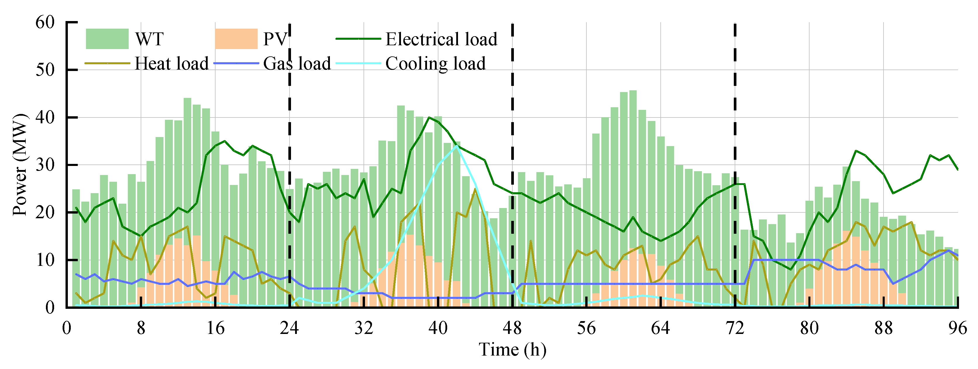
The WT/PV generation profiles and the load demand curves are shown in Figure 2.

The multi-timescale coupling contains two complementary channels. The first is an information channel. Historical WT, PV, and multi-energy load data are used to determine seasonal carbon-pressure factors, which are then mapped to the corresponding 24 h representative segments. Within each segment, the assigned factor modifies the hourly carbon-embedded energy prices, and these prices influence the demand response loads and subsequent dispatch decisions.

The second is a physical-state channel. The terminal SGS state of each seasonal segment is transferred to the following segment as its initial state, thereby linking gas storage decisions across spring, summer, autumn, and winter. Carbon allowances and physical emissions are calculated at the same hourly resolution as the energy dispatch and accumulated over the modeled 96 h horizon.

The 96 h horizon consists of four 24 h representative profiles for typical spring, summer, autumn, and winter days. They are placed in one computational horizon for comparison and should not be interpreted as four consecutive calendar days. The model does not assign annual weights to the profiles or represent the actual elapsed time, monthly accumulation, or long-term self-discharge between seasons. Seasonal carbon-pressure factors affect each hourly segment through carbon-embedded prices and demand response, while linked SGS boundary states provide a simplified representation of gas inventory coordination across the four segments. Accordingly, the results describe four seasonal representative days rather than a complete chronological year.

To quantify the respective effects of the carbon–energy trading mechanism, the low-carbon energy demand response strategy, and the seasonal scheduling strategy, five comparative scenarios are established:

Scenario 1: The conventional market mechanism is adopted without low-carbon energy demand response or seasonal scheduling.

Scenario 2: The carbon–energy integrated market mechanism is introduced, while low-carbon energy demand response and seasonal scheduling are not considered.

Scenario 3: On the basis of Scenario 2, the low-carbon energy demand response strategy is further incorporated, whereas seasonal scheduling is not considered.

Scenario 4: The conventional market mechanism is retained, and seasonal scheduling is considered without low-carbon energy demand response.

Scenario 5: The complete proposed framework is adopted, including the carbon–energy integrated market mechanism, low-carbon energy demand response, and seasonal scheduling.

5.2. Analysis of the Results of the Low-Carbon Energy Demand Response Strategy

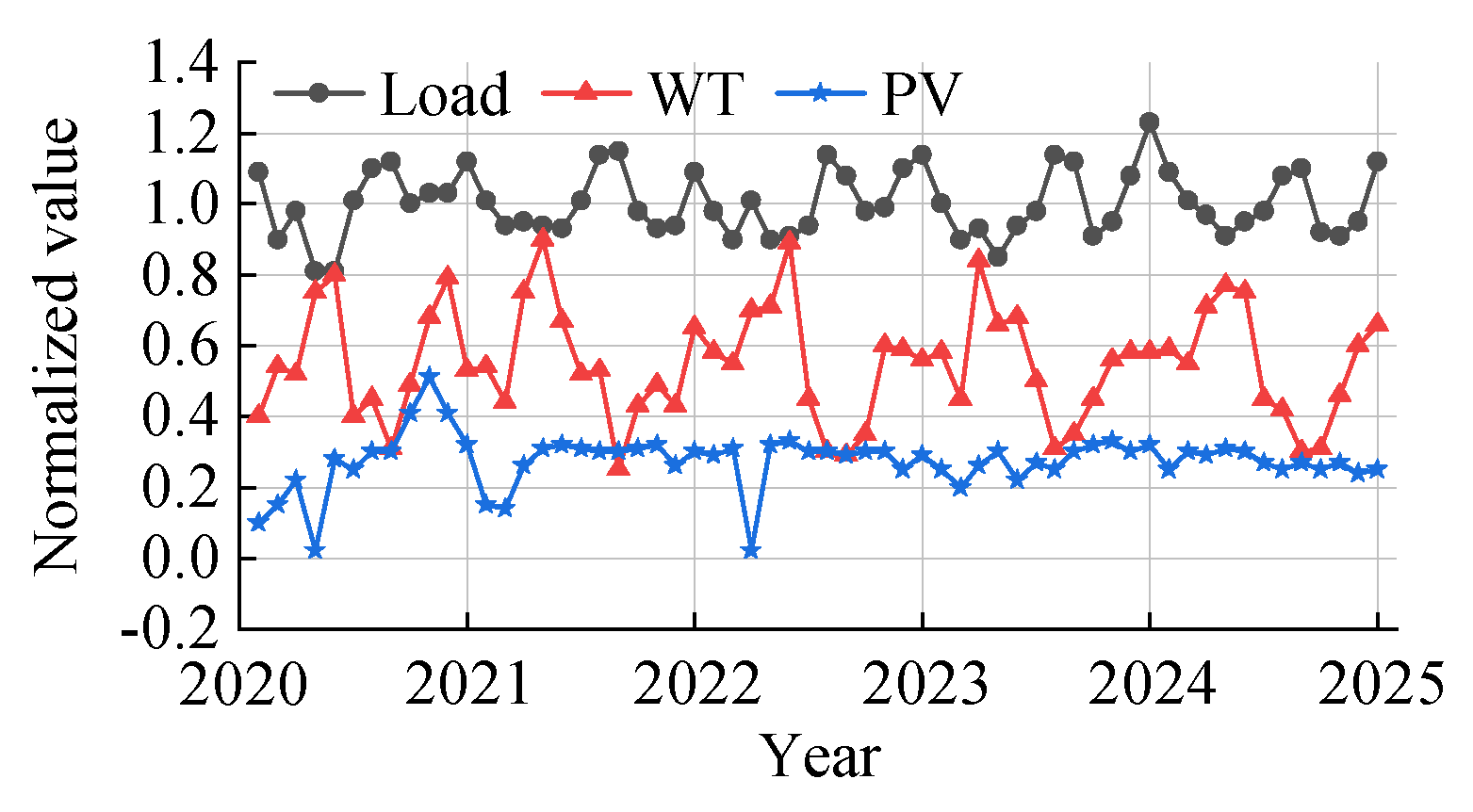
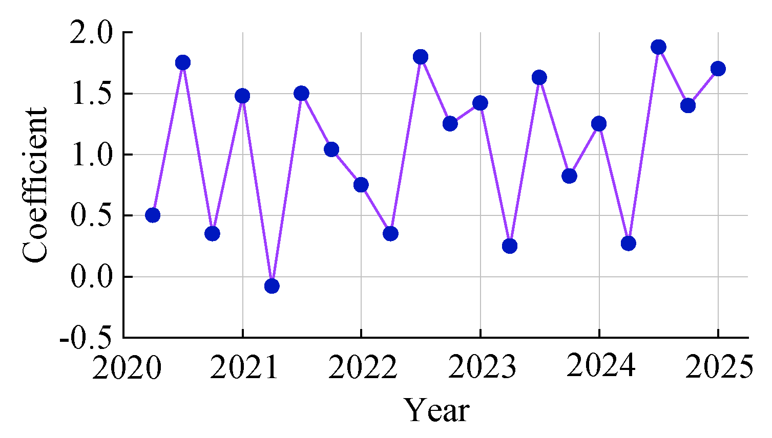
The normalized WT, PV, and load data for 2020–2025 are shown in Figure 3, and the corresponding seasonal carbon emission indicators are shown in Figure 4. Within each year, the four observations represent spring, summer, autumn, and winter in that order.

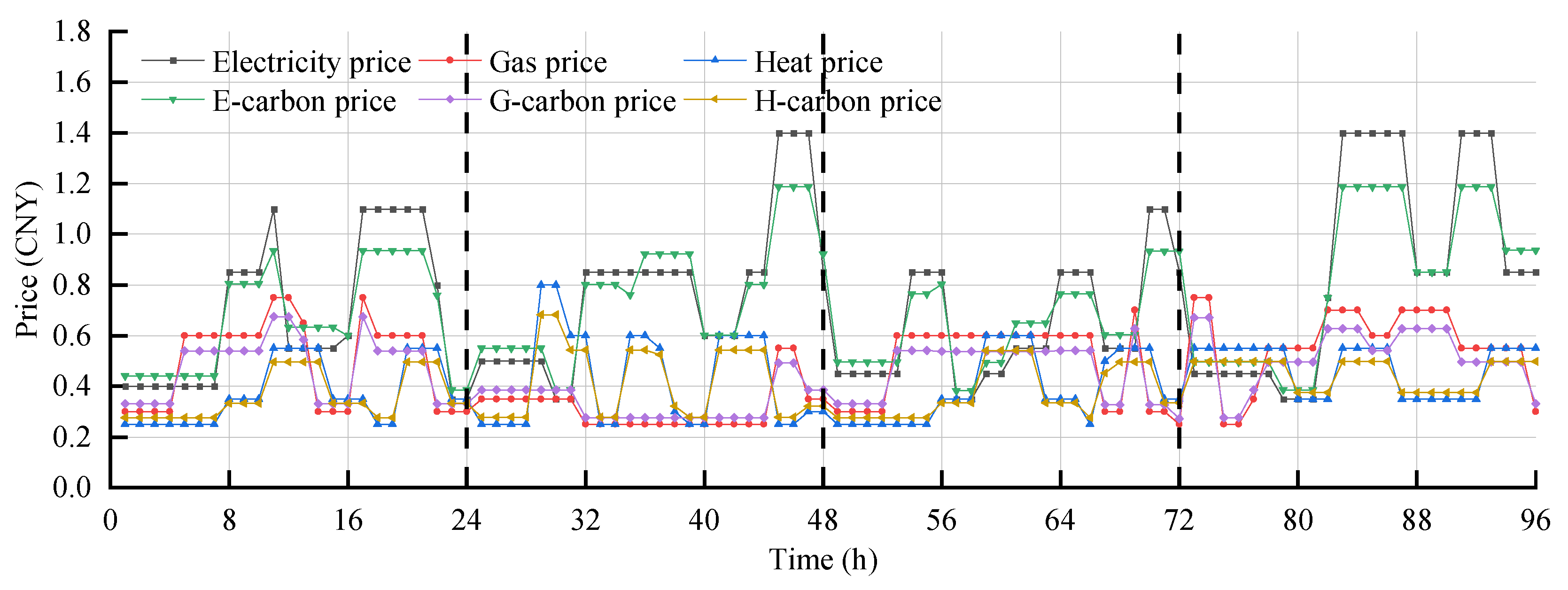
Applying the procedure in Section 3.2.1 gives carbon-pressure factors of 0.061, 0.399, 0.241, and 0.301 for spring, summer, autumn, and winter, respectively. Figure 5 compares the conventional energy prices with the carbon-embedded electricity, gas, and heat prices over the four representative days. The carbon trading incentive–disincentive term introduces a modest adjustment to the base energy price, and the seasonal factor scales that adjustment according to the historical carbon-pressure pattern. The resulting prices provide differentiated hourly signals for demand response; they do not represent a separate carbon market settlement.

Table 5. Proportions of shiftable and curtailable loads.

Load Demand Types	Curtailable-Load Proportion	Shiftable-Load Proportion
Electric Load	0.6%	4.8%
Gas Load	0.6%	4.8%
Heat Load	0.4%	3.9%

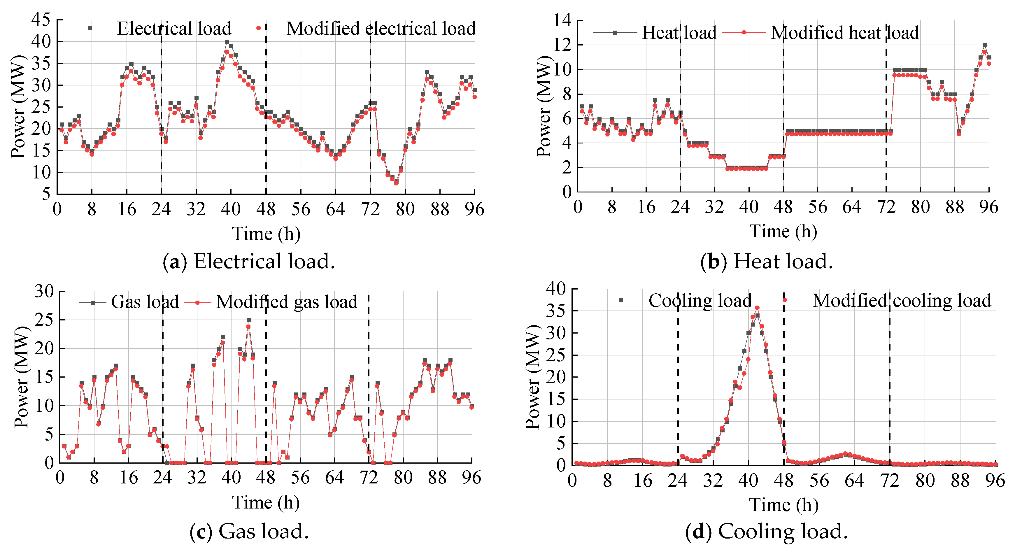
lists the curtailable and shiftable shares of the electricity, gas, and heat loads. Figure 6 shows the corresponding electricity, heat, gas, and cooling profiles before and after demand response.

Figure 6 shows that the seasonal carbon-pressure factors lead to different response intensities across the four representative days. Within a given day, adjustable demand responds to the corresponding hourly carbon-embedded prices; no end-use load is transferred from one season to another. Because the shiftable share is small and its daily energy is conserved, the dominant effect is intra-day smoothing. Reductions in average demand come instead from curtailable demand and the bounded cooling adjustment.

Cooling demand is described by the building thermal-balance equation, an offline piecewise-linear approximation of the PMV relation, and explicit limits on temperature, PMV, and load adjustment. The model therefore captures bounded, comfort-aware flexibility under the adopted assumptions. It is not a real-time adaptive fuzzy controller.

Table 6. Load statistics before and after low-carbon demand response.

	Load Type	Average Value (MW)	Variance (MW2)
Before demand response	electrical load	23.73	47.8895
	heat load	5.65	5.7962
	gas load	8.85	42.4356
	cooling load	3.90	62.4105
After demand response	electrical load	22.27	42.9193
	heat load	5.30	5.1848
	gas load	8.46	38.3171
	cooling load	3.83	60.0951

shows variance reductions of 10.38%, 10.54%, 9.71%, and 3.71% for the electricity, heat, gas, and cooling loads, respectively. These changes indicate smoother intra-day profiles. The lower average values are caused by curtailment and the bounded cooling adjustment; shiftable demand does not alter the daily total because its energy is conserved within each representative day.

5.3. Comparative Analysis of Operation Results in Different Scenarios

To implement the compromise-selection procedure in Section 4.3, the economic and carbon emission objectives were first minimized separately. The two single-objective solutions provide the ideal values and the approximate nadir values used for normalization.

A real-coded IGA was then used to search for the economic preference weight $\beta$, while the carbon emission weight was calculated as $1-\beta$. The population size was set to 20, and the maximum number of generations was 50. The crossover and mutation probabilities were 0.8 and 0.1, respectively. The outer IGA terminated when the maximum number of generations was reached or when the improvement in the best fitness was below 10⁻⁴ for eight consecutive generations. Each inner mixed-integer linear programming problem was solved using CPLEX with a relative optimality gap of 10⁻⁴ and a maximum solution time of 300 s. Boundary repair and elitist preservation were applied during each generation.

Because β is the only independent preference variable, a deterministic scan was used to verify the stochastic IGA result. The admissible interval was first evaluated with a step of 0.01 and then refined with a step of 0.001 around the minimum-distance region. The deterministic scan selected β = 0.621, consistent with the IGA result of approximately 0.62.

The resulting operating cost and carbon emissions were normalized, and the fitness of the chromosome was evaluated according to its distance from the economic-environmental ideal point. Boundary repair was performed after crossover and mutation to maintain feasible weights, and an elitist preservation strategy was used to retain the candidate with the highest fitness.

The IGA was run independently 30 times with different random seeds. The mean selected economic weight was 0.621, with a standard deviation of 0.006, and 93.3% of the runs fell within ±0.01 of the deterministic-scan result. The average convergence generation was 21.8.

Table 7. Convergence history of the IGA over 30 independent runs.

Generation	Mean Best Ideal-Point Distance	Standard Deviation	Mean Economic Weight
1	0.4920	0.0260	0.574
5	0.4510	0.0180	0.596
10	0.4340	0.0110	0.612
15	0.4270	0.0070	0.618
20	0.4254	0.0040	0.620
25	0.4251	0.0030	0.621
30	0.4250	0.0030	0.621

summarizes the convergence history.

Table 8. Sensitivity of the IGA to population size and mutation probability.

Population Size	Mutation Probability	Mean β	Standard Deviation	Mean Convergence Generation
10	0.10	0.618	0.012	26.4
20	0.05	0.619	0.008	23.7
20	0.10	0.621	0.006	21.8
20	0.20	0.623	0.010	23.1
40	0.10	0.620	0.004	19.6

reports the sensitivity of the IGA to population size and mutation probability. The mean ideal-point distance decreases rapidly during the first 15 generations and changes only slightly after about 20 generations, while the mean economic weight approaches 0.621 and its dispersion narrows. This supports numerical convergence under the adopted settings, not the identification of a unique decision-maker preference.

The selected economic weight remains close to 0.62 under all tested parameter settings. Increasing the population size reduces run-to-run dispersion but requires more inner CPLEX evaluations. A mutation probability of 0.10 provides a reasonable balance between convergence speed and numerical stability for the present case.

Table 9. Cost–emission trade-off obtained from deterministic weight scanning.

Economic Weight β	Operating Cost (CNY)	Carbon Emissions (t)	Normalized Ideal-Point Distance
0.00	948,000.00	930.00	1.000
0.20	933,800.00	936.50	0.792
0.40	918,900.00	947.80	0.587
0.50	910,600.00	956.90	0.493
0.60	901,600.00	968.00	0.426
0.62	900,485.52	970.24	0.425
0.70	894,700.00	984.60	0.461
0.80	888,700.00	1002.50	0.556
1.00	880,000.00	1064.13	1.000

shows the cost–emission trade-off from deterministic weight scanning. Increasing the economic weight generally lowers operating cost and raises emissions. The minimum normalized ideal-point distance occurs near β = 0.62. This point is selected under the adopted normalization and Euclidean-distance criterion and is not an objectively or uniquely preferred solution.

The proposed procedure was also compared with deterministic grid search, the ε-constraint method, NSGA-II, MOEA/D, and MOPSO. All methods used the same system data, objective normalization, operating constraints, and CPLEX-based dispatch evaluation. Population-based methods were repeated with independent random seeds, whereas deterministic methods were run once.

Table 10. Comparison of compromise solutions obtained by different methods.

Method	Equivalent Economic Weight	Operating Cost (CNY)	Carbon Emissions (t)	Normalized Ideal-Point Distance
Equal weighting	0.500	910,600.00	956.90	0.4930
Deterministic grid search	0.621	900,485.52	970.24	0.4250
ε-constraint	≈0.610	900,920.00	969.80	0.4258
NSGA-II	≈0.620	901,050.00	969.60	0.4266
MOEA/D	≈0.618	900,760.00	969.95	0.4254
MOPSO	≈0.623	901,180.00	969.30	0.4278
IGA–CPLEX	0.621	900,485.52	970.24	0.4251

compares the selected compromise solutions, and

Table 11. Computational and statistical comparison of the optimization methods.

Method	Independent Runs	Dispatch Evaluations	Mean Time (s)	Weight/Solution Dispersion
Deterministic grid search	1	122	214.7	—
ε-constraint	1	51	188.3	—
NSGA-II	30	1000	438.6 ± 26.2	0.620 ± 0.009
MOEA/D	30	800	401.5 ± 21.7	0.618 ± 0.007
MOPSO	30	1000	472.8 ± 34.9	0.623 ± 0.011
IGA–CPLEX	30	436	268.4 ± 11.6	0.621 ± 0.006

reports the computational and statistical results.

The deterministic grid search, ε-constraint method, and population-based algorithms all identified compromise solutions within a narrow economic–environmental trade-off region. The economic weights corresponding to the selected solutions ranged from approximately 0.61 to 0.623, while the differences in operating cost and carbon emissions remained below 0.08% and 0.10%, respectively.

The deterministic grid search provided the clearest reproducibility benchmark for the present one-dimensional problem. The ε-constraint method generated a transparent nondominated set with relatively low computational effort. NSGA-II, MOEA/D, and MOPSO offered broader Pareto-front information but required more dispatch evaluations and repeated stochastic runs. Among the tested population-based methods, MOEA/D showed slightly lower dispersion and computational time than NSGA-II and MOPSO.

The IGA–CPLEX procedure produced a compromise consistent with the deterministic benchmark and required less computation than the three population-based multi-objective algorithms. Nevertheless, this result does not establish the general superiority of IGA. Its main advantage in the present framework is the direct separation between the outer preference search and the inner mixed-integer dispatch model.

Under these parameter settings, the IGA converged to an economic weight of 0.62 and a carbon emission weight of 0.38. These weights were fixed in all five comparative scenarios. In addition, the same representative WT and PV output profiles were used in all scenarios. Therefore, the differences reported in

Table 12. Optimized operating results for the five scenarios.

Scenario	Carbon Emissions (t)	Operating Costs (CNY)
Scenario 1	1052.92	1,103,420.84
Scenario 2	1052.73	1,102,623.89
Scenario 3	1014.90	971,851.56
Scenario 4	1028.50	1,066,301.65
Scenario 5	970.24	900,485.52

reflect the effects of the market mechanism, demand response strategy, and seasonal scheduling strategy, rather than changes in the renewable generation inputs or objective preferences. The optimized operating results under the five comparative scenarios are presented in Table 12.

Scenario 2 changes little relative to Scenario 1: operating cost falls by CNY 796.95 and carbon emissions by 0.19 t, or only 0.072% and 0.018%. The carbon–energy pricing mechanism therefore has limited practical influence when used by itself. Its value lies mainly in providing differentiated signals that become more effective when demand response and seasonal storage scheduling are also available. The comparison of Scenarios 2 and 3 confirms this interaction, because adding low-carbon demand response produces further reductions in both cost and emissions.

The comparison between Scenarios 1 and 4 shows that seasonal scheduling can also reduce cost and emissions under the conventional carbon-market setting. Scenario 5 performs better than Scenario 1 under the adopted case-study conditions, but the improvement is obtained with additional constraints and computational effort. The result should therefore be interpreted as a day-ahead scheduling outcome rather than a general operational guarantee.

Scenario 5 extends Scenario 3 by adding the seasonal scheduling link while keeping the same carbon–energy market and demand-response settings. Scenario 4 provides the corresponding seasonal-scheduling comparison under the conventional market. The larger improvement from Scenario 3 to Scenario 5 suggests that inter-segment inventory coordination is more useful when carbon-embedded prices and flexible demand operate together. By contrast, Scenarios 4 and 5 differ in both market and demand-response settings, so that comparison cannot isolate a single mechanism.

The scenario comparison indicates that SGS inventory is shifted toward the representative summer and winter segments, when the carbon-pressure factors are higher, and replenished in the spring and autumn segments, when the factors are lower. This reduces high-carbon external electricity purchases within the modeled horizon. The park-level IES contains no local coal-fired unit; the gas- and coal-fired shares appear only in the upstream grid-emission coefficient. The SGS result should therefore be read as inter-segment gas inventory coordination, not as a verified reduction in local coal-unit operating time.

Compared with the other scenarios, Scenario 5 combines seasonal carbon-pressure information, linked SGS inventory states, carbon-embedded prices, and flexible demand in one 96 h representative horizon. Hourly feasibility is maintained within each segment, while the linked SGS states coordinate gas inventory across the four representative profiles. This is a model-based inter-segment result rather than a chronological demonstration of annual cross-seasonal operation.

Table 13. Breakdown of the operating cost under different scenarios.

Scenario	Energy-Purchase Cost	Conversion Cost	Storage Cost	Carbon Trading Payment	DR Compensation
Scenario 1	879,846.37	150,284.61	34,912.48	38,377.38	0.00
Scenario 2	879,214.56	150,118.73	34,968.42	38,322.18	0.00
Scenario 3	752,438.29	139,684.75	38,127.64	29,163.32	12,437.56
Scenario 4	826,742.18	146,293.47	50,864.59	42,401.41	0.00
Scenario 5	689,742.63	131,847.29	47,936.58	18,215.47	12,743.55

provides the operating cost breakdown. The largest reduction in Scenario 5 comes from lower external energy-purchase cost. Storage operation and demand response compensation add cost, but these increases are offset by lower energy-purchase, conversion, and carbon settlement costs.

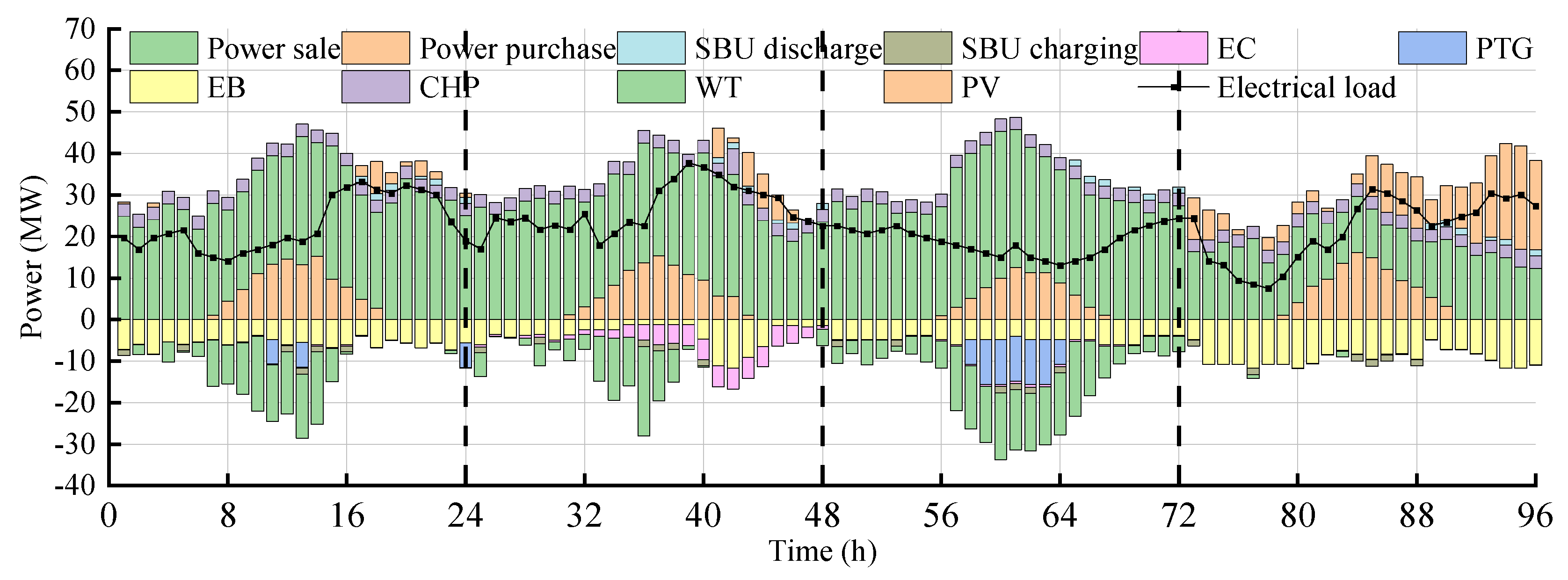
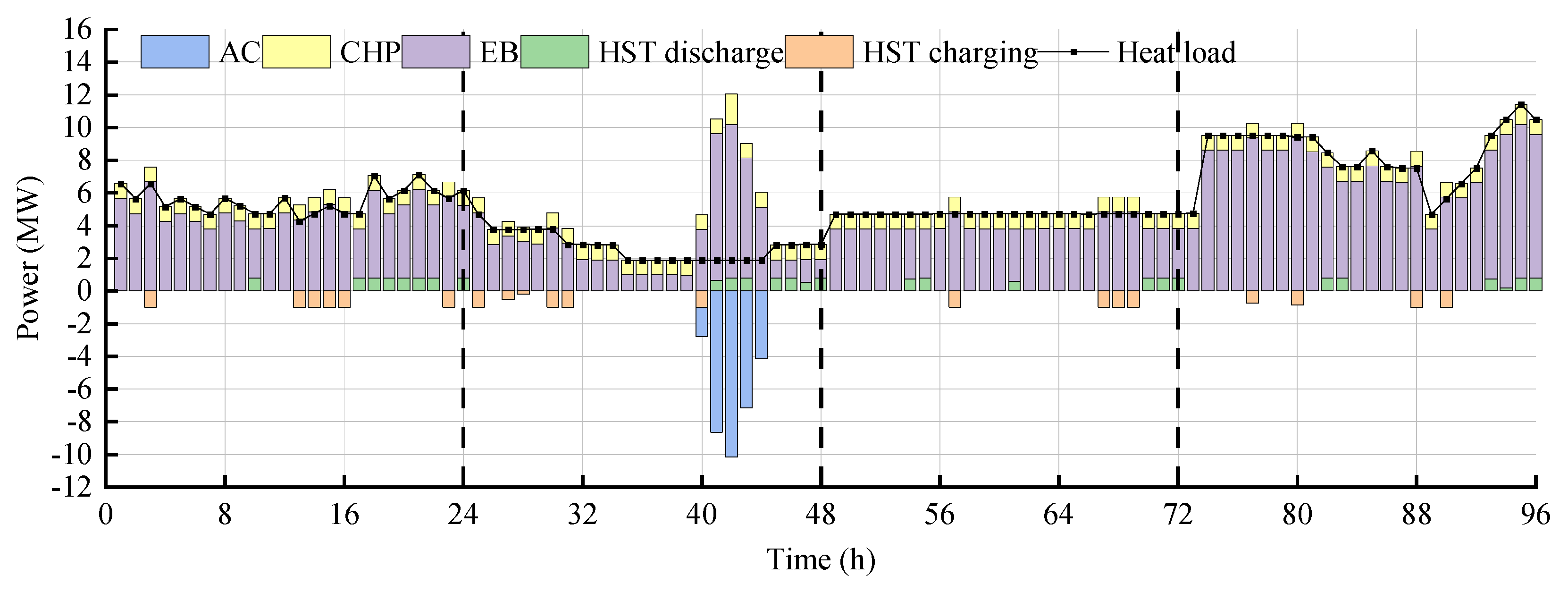
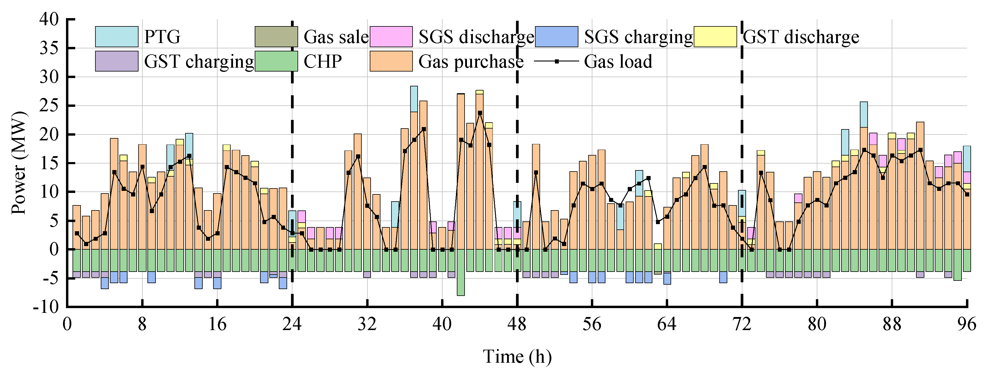
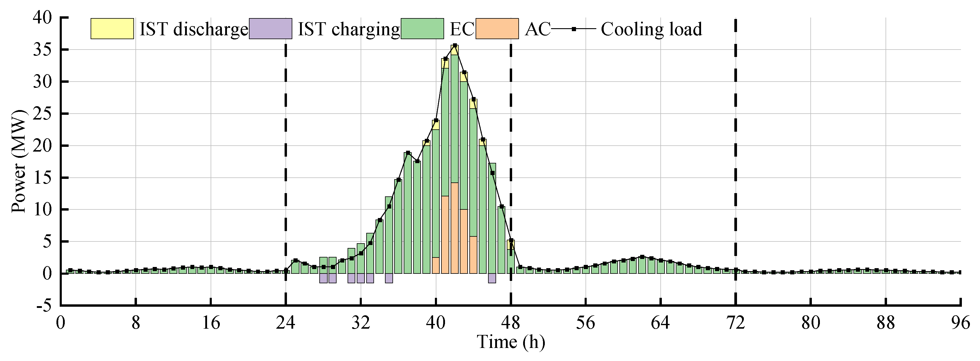
Figure 7 shows that surplus renewable output allows electricity export during parts of the spring, summer, and autumn profiles, whereas the winter profile requires more grid electricity to support heating. Figure 8 indicates that EB and CHP are the main heat sources. Figure 9 shows the gas balance, including gas-grid exchange and P2G conversion, and Figure 10 shows that cooling demand is concentrated in the summer profile and is supplied mainly by EC with support from AC. 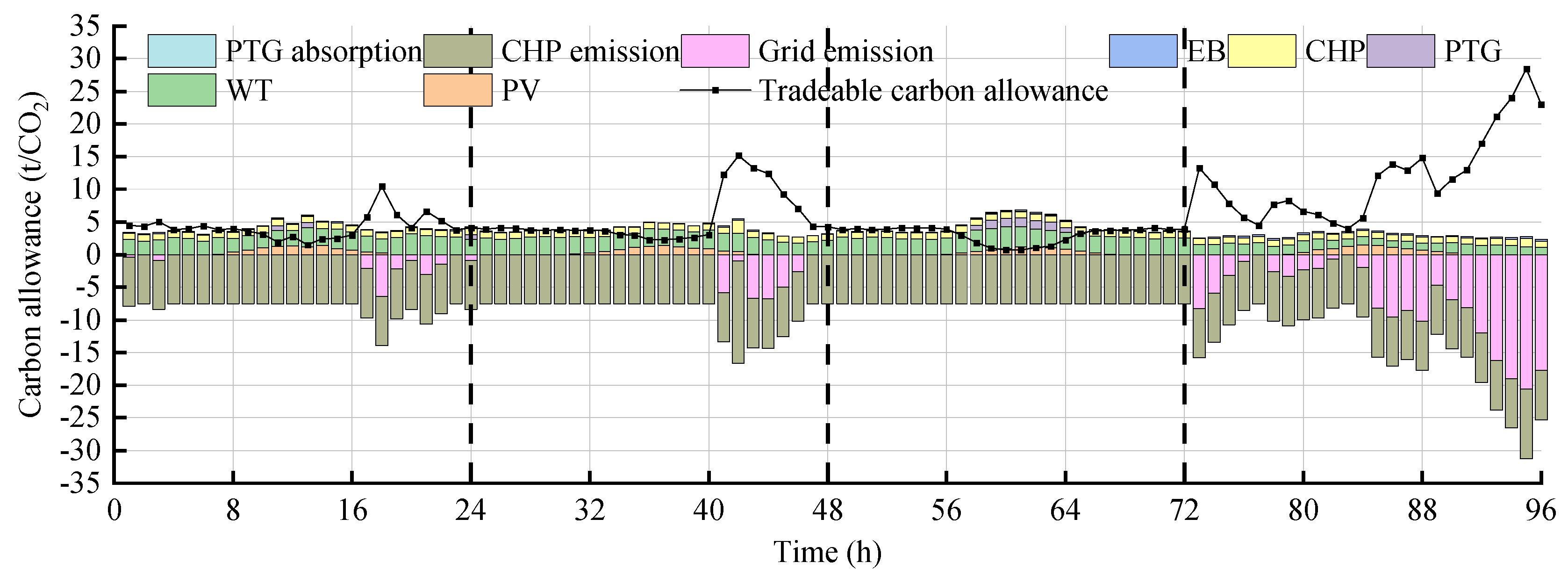Figure 11 presents the modeled carbon-accounting balance. Purchased allowances increase in the winter profile, while surplus allowances are sold in some other periods. These trajectories illustrate the settlement behavior of the model under the adopted inputs; they do not independently validate the market mechanism.

It should be noted that Figure 11 contains both physical emission terms and allowance allocation terms. “CHP emission” and “Grid emission” represent physical carbon emissions, whereas the quantities associated with EB, CHP, P2G, WT, and PV represent internally allocated carbon allowances.

5.4. Analysis of Energy Storage State-of-Charge Trajectories

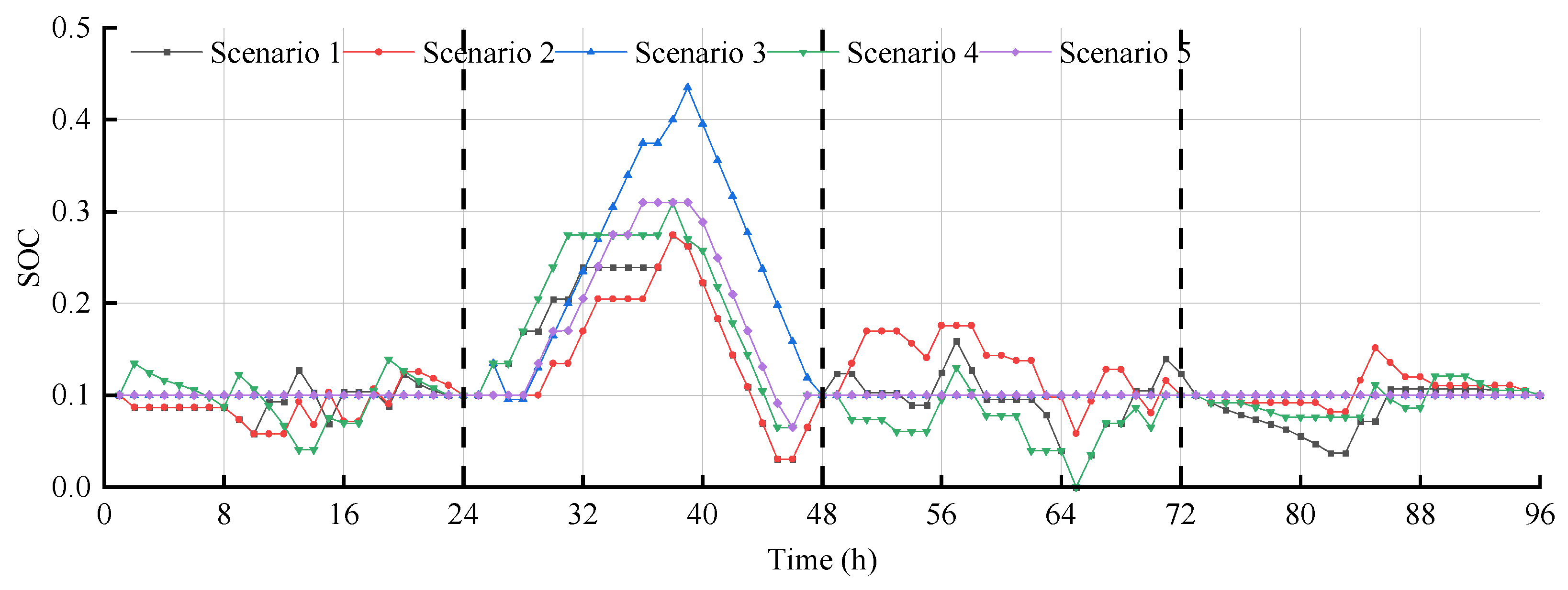
In the present representative-day model, the SGS state is connected among the four seasonal operating profiles to examine the influence of storage inventory coordination under different seasonal source–load and carbon-pressure conditions. This connection is a simplified inter-profile inventory relationship and does not represent the physical elapsed time or storage loss occurring over several months.

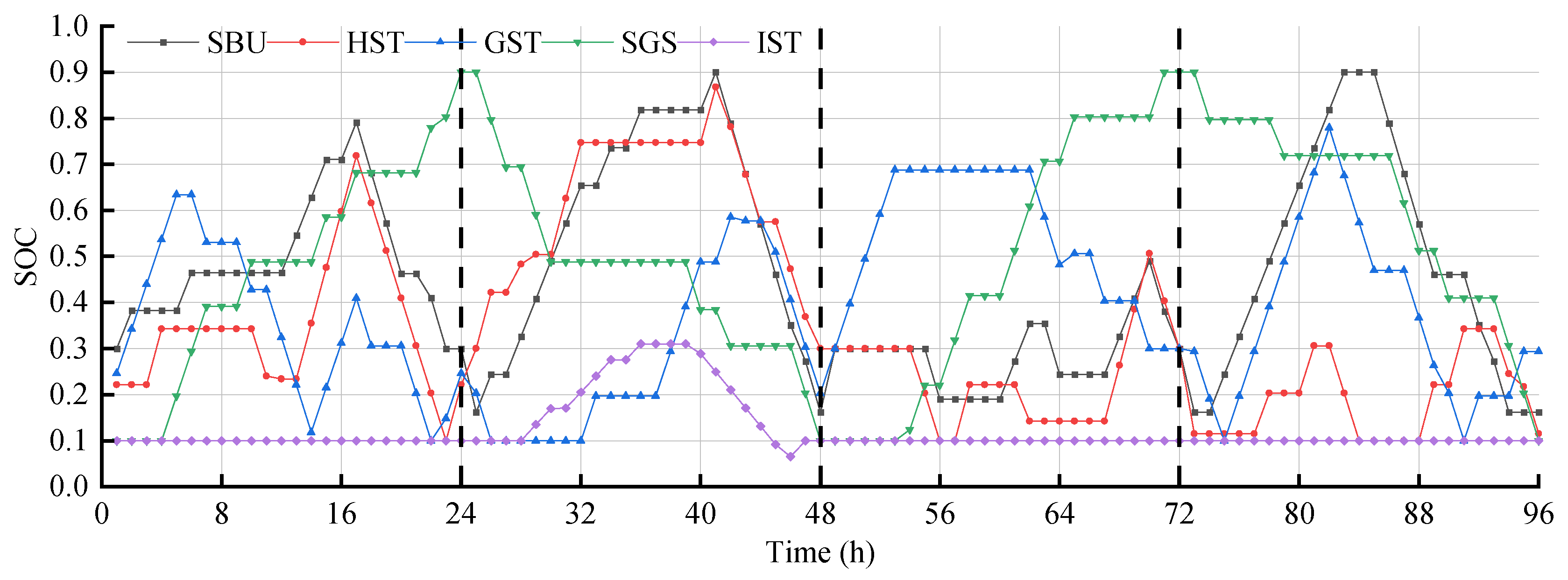
To enhance economic performance, multiple energy storage devices in the IES are employed to smooth renewable energy output and participate in peak–valley price arbitrage, as illustrated in Figure 12.

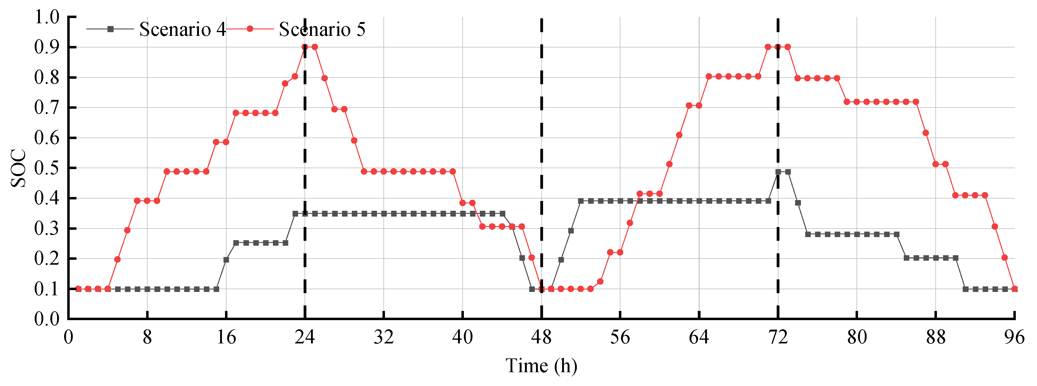
SBU, HST, and GST primarily operate following the peak–valley distribution of carbon–energy prices, charging during off-peak periods and discharging during peak periods to achieve load leveling. Cooling energy, converted from electricity and thermal energy, exhibits a similar peak–valley response. SGS operates in accordance with seasonal carbon-pressure factors, charging on typical spring and autumn days with lower low-carbon demand signals and discharging on typical summer and winter days with higher low-carbon demand signals. These trajectories show that, within the four representative seasonal segments, SGS is scheduled to charge during spring and autumn and discharge during summer and winter. This result represents modeled gas redistribution across the representative horizon rather than verified annual cross-seasonal operation.

Figure 13 shows that IST activity is concentrated more strongly around the summer cooling period in Scenarios 3 and 5 than in Scenarios 1, 2, and 4. Figure 14 shows that the SGS state-of-charge range expands from approximately 0.1–0.5 in Scenario 4 to 0.1–0.9 in Scenario 5. Because Scenarios 4 and 5 differ in both market and demand response settings, the wider range reflects their combined influence under the complete framework. No claim about reduced storage losses, equipment protection, or service-life extension is made because degradation and reliability are not modeled.

The storage results reported in this section describe only the optimized charging, discharging, and state-of-charge trajectories. Since degradation, cycling-dependent losses, lifetime, and reliability are not explicitly modeled, no quantitative conclusions regarding equipment protection or service-life extension are drawn from these results.

5.5. Sensitivity Analysis and Practical Implementation

Scenario 5 is used as the baseline for a one-factor-at-a-time sensitivity analysis, with an operating cost of CNY 900,485.52 and cumulative carbon emissions of 970.24 t over the representative horizon. Carbon price, renewable generation share, aggregate storage capacity, demand response participation, and seasonal carbon-pressure intensity are varied from 80% to 120% of their baseline values. Objective weights are evaluated separately, with all other parameters fixed.

Table 14. One-factor-at-a-time sensitivity results under Scenario 5.

Sensitivity Factor	Parameter Level	Operating Cost (CNY)	Cost Change	Carbon Emissions (t)	Emission Change
Baseline	1.00	900,485.52	0.00%	970.24	0.00%
Carbon price	0.80	892,200.00	−0.92%	983.60	1.38%
	1.20	910,800.00	1.15%	956.30	−1.44%
Renewable generation share	0.80	934,600.00	3.79%	1004.80	3.56%
	1.20	872,900.00	−3.06%	939.70	−3.15%
Aggregate storage capacity	0.80	915,700.00	1.69%	981.90	1.20%
	1.20	892,600.00	−0.88%	962.50	−0.80%
Demand response participation	0.80	908,900.00	0.93%	977.40	0.74%
	1.20	894,300.00	−0.69%	965.80	−0.46%
Seasonal carbon-pressure intensity	0.80	897,200.00	−0.36%	978.50	0.85%
	1.20	904,900.00	0.49%	963.20	−0.73%
Objective weights	0.75/0.25	889,500.00	−1.22%	985.80	1.60%
	0.50/0.50	916,700.00	1.80%	950.90	−1.99%

Note: The objective weight combinations are reported as economic weight/carbon emission weight. A parameter level of 1.00 represents the baseline setting.

reports the sensitivity results.

The renewable generation share produces the largest variation in both evaluation indicators. A 20% reduction in renewable output increases the operating cost and carbon emissions by 3.79% and 3.56%, respectively, whereas a 20% increase reduces them by 3.06% and 3.15%. This result indicates that renewable availability is a major determinant of system performance.

Increasing the carbon price reduces physical carbon emissions but raises the operating cost, reflecting a clear economic–environmental trade-off. A similar relationship is observed for the objective weights. Increasing the carbon emission weight from 0.38 to 0.50 reduces emissions by 1.99%, although the operating cost increases by 1.80%. Therefore, the selected weight combination should be interpreted as a compromise rather than a universally optimal setting.

Storage capacity and demand response participation have moderate effects. Reducing either parameter causes a larger deterioration than the improvement obtained from an equivalent increase, suggesting diminishing marginal benefits near the baseline configuration. The seasonal carbon-pressure intensity has a relatively limited effect on the aggregate results, with changes below 1%, but it affects the timing of load adjustment and SGS charging and discharging.

5.6. Practical Benefits and Computational Effort

Across the modeled representative horizon, Scenario 5 reduces operating cost from CNY 1,103,420.84 to CNY 900,485.52 and carbon emissions from 1052.92 t to 970.24 t relative to Scenario 1. The corresponding reductions are 18.39% and 7.85%.

These gains come with a more detailed model. The seasonal carbon-pressure factors are calculated before optimization and add no decision variables. Most of the extra computational burden arises from flexible-load variables, cooling-comfort constraints, inter-segment SGS state equations, and the repeated inner solves required for compromise-weight selection.

Across ten runs, the mean solution times were 9.6 s for Scenario 1, 17.8 s for Scenario 5 with fixed weights, and 268.4 s for the complete IGA–CPLEX procedure. The nested method is slower because every candidate weight triggers an inner dispatch solve. In practice, the weight search can be performed offline or repeated only after a material change in market conditions or operating preferences; routine scheduling can then use the fixed-weight model.

Table 15. Computational performance of different solution modes.

Solution Mode	Average Time (s)	Standard Deviation (s)
Scenario 1	9.6	0.8
Scenario 5 with fixed weights	17.8	1.4
Complete IGA–CPLEX procedure	268.4	11.6

and

Table 16. Computational performance for different scheduling horizons.

Scheduling Horizon	Fixed-Weight Dispatch Time	Complete IGA–CPLEX Time
24 h	5.1 s	79.4 s
48 h	9.2 s	145.7 s
96 h	17.8 s	268.4 s
192 h	36.9 s	553.6 s

summarize the timing results for the solution modes and scheduling horizons.

Fixed-weight dispatch time increases approximately linearly with the scheduling horizon. The complete nested procedure grows more rapidly because each IGA candidate requires a mixed-integer dispatch solution. Even so, the tested 192 h case is solved in about 10 min under the reported configuration.

For deployment, seasonal carbon-pressure factors and compromise weights can be updated offline or whenever market conditions change materially. Routine operation then requires only the fixed-weight dispatch calculation. This separation limits the online burden and supports day-ahead or periodically updated scheduling. Scalability to much larger systems—with more devices, network constraints, or uncertainty scenarios—still needs to be tested.

The method provides a practical interface between seasonal carbon-management information and hourly IES operation. Historical renewable-generation and load data can be used to recalibrate the seasonal factors, while renewable forecasts, market prices, equipment states, and state-of-charge values update the hourly schedule.

The reported cost and emission reductions remain conditional on the representative horizon and parameter settings. Field deployment would also require reliable metering and communication, formal demand-response agreements, and periodic calibration with operating data.

5.7. Practical Implementation and Deployment Limitations

Practical implementation requires both historical and operational data. Historical WT, PV, and multi-energy load records are used to estimate seasonal carbon-pressure factors. Routine scheduling additionally requires short-term renewable and load forecasts, electricity and gas prices, carbon prices and allowance information, equipment availability, conversion efficiencies, SOC values, indoor temperature measurements, and the available demand response capacity. The seasonal factors may be recalibrated periodically, whereas the operating inputs should be updated before each scheduling cycle.

The proposed model can be integrated into an energy management system operated by a park-level energy manager or aggregator. Smart meters collect electricity, heat, gas, and cooling data, while equipment controllers report operating states and storage levels. The optimization results are transmitted to local controllers as unit schedules, storage charging or discharging commands, and demand response instructions. Reliable time synchronization, two-way communication, data quality checks, and fallback operating rules are required before automatic implementation.

Demand response also depends on contractual arrangements with participating users. The permissible adjustment range, response duration, compensation mechanism, comfort limits, and opt-out conditions should be specified in advance. Carbon settlement requires traceable metering and a measurement, reporting, and verification procedure that distinguishes allocated allowances from physical emissions.

Several limitations remain. The current dispatch model uses fixed representative renewable profiles and does not explicitly optimize forecast error recourse. It also represents the IES in an aggregated form without detailed electricity, heat, or gas network constraints. In addition, elasticity coefficients and comfort parameters require local calibration, while market access and carbon settlement rules may differ across regions. Communication failures, cybersecurity risks, and data privacy requirements may further restrict fully automated deployment. The framework is therefore intended for day-ahead or periodically updated scheduling rather than second-level operational control.

5.8. Discussion of Performance Mechanisms and Limitations

The performance of the complete framework cannot be assigned to one component alone. Carbon-embedded prices create time-varying signals for flexible electricity, heat, and gas loads, moving part of the demand away from periods with higher cost and carbon pressure. SBU, HST, GST, and IST coordinate supply and demand within each representative day, while SGS adds flexibility across the four seasonal segments. The comfort-constrained cooling model brings cooling demand into the dispatch problem without exceeding the prescribed PMV and load-adjustment limits. Together, these mechanisms reduce unfavorable external energy purchases and improve coordination among renewable generation, conversion units, and storage.

These results must be read within the stated model boundary. The analysis uses four unweighted seasonal representative days, and the reported cost and emission values are cumulative results for a 96 h horizon, not annual estimates. Renewable profiles become fixed inputs after scenario preprocessing, so forecast errors and recourse decisions are not optimized explicitly. The IES is represented as an aggregated energy hub without detailed electricity, heat, or gas network constraints. Elasticity coefficients, comfort parameters, and equipment characteristics would also need site-specific calibration.

The ideal-point criterion selects a model-dependent compromise weight; it does not recover a unique stakeholder preference. The full IGA–CPLEX procedure also requires more computation, although the weight search can be conducted offline. Future work will examine weighted annual representative periods, rolling and stochastic scheduling, detailed multi-energy networks, storage degradation, field-calibrated demand response, and decomposition or parallel solution methods for larger systems.

5.9. Implications for Sustainability

The sustainability contribution can be expressed as a measurement–signal–response–dispatch chain. Historical renewable-output and demand data are converted into seasonal carbon-pressure factors. The factors modify hourly carbon-embedded prices, and those prices influence demand response, energy conversion, storage operation, external exchange, and carbon accounting. The practical idea is simple: medium- and long-term carbon information becomes usable in day-ahead dispatch without changing the one-hour scheduling resolution.

The numerical results also show why the mechanisms should be evaluated as a coordinated package. Carbon-embedded pricing has only a small effect when applied alone, but its influence increases when flexible demand and seasonal gas-storage coordination are added. Under the complete framework, emissions and operating cost fall by 7.85% and 18.39%, respectively, relative to Scenario 1. These percentages are case-specific, not universal. They demonstrate that, under the adopted conditions, environmental and economic performance can improve together when market signals, storage, and user-side response are optimized in one model.

At the park level, the framework also supports monitoring and governance. Seasonal factors can be recalibrated from historical data, and forecasts, market and carbon prices, allowance information, equipment states, storage levels, indoor temperatures, and available response capacity can be updated before each scheduling cycle. An energy manager or aggregator can translate the optimized solution into unit schedules, storage commands, and demand-response instructions. Field use would still depend on reliable metering and communication, data-quality procedures, user agreements, and traceable measurement, reporting, and verification for carbon settlement.

The sustainability interpretation is deliberately limited. Four unweighted seasonal profiles form the 96 h horizon, so the reported reductions are not annual indicators and do not constitute a complete social-welfare or life-cycle assessment. Renewable forecast errors, detailed network constraints, storage degradation, and locally calibrated behavioral parameters are not fully represented. Stronger long-term claims will require weighted annual or rolling studies, uncertainty modeling, site-specific calibration, and field validation.

6. Conclusions

This paper develops a multi-timescale low-carbon economic scheduling framework for a multi-energy IES. It extends an inherited seasonal carbon-pricing and storage model by adding comfort-aware cooling response and a reproducible compromise-weight selection procedure. The main findings are as follows:

(1)

Seasonal carbon-pressure factors carry historical seasonal information into hourly prices and demand response, while linked SGS boundary states coordinate gas inventory across the four representative segments. This is a simplified redistribution within the 96 h horizon, not a chronological annual storage trajectory.

(2)

The PMV-constrained cooling demand-response model incorporates thermal-comfort limits into load adjustment. Under the adopted settings, the variances of the electricity, heat, gas, and cooling loads decrease by 10.38%, 10.54%, 9.71%, and 3.71%, respectively. These values describe changes in the optimized load profiles; they are not experimental proof of comfort preservation.

(3)

Using the ideal-point distance criterion, the IGA–CPLEX framework selects economic and carbon-emission weights of 0.62 and 0.38. Relative to Scenario 1, the complete framework reduces carbon emissions by 7.85% and operating cost by 18.39%. The selected weights represent one model-dependent compromise rather than objectively identified stakeholder preferences.

Taken together, the method links emission reduction, operating economy, renewable-energy coordination, storage utilization, demand-side flexibility, and user comfort in one decision process. It gives park-level energy managers and aggregators a measurable way to translate carbon-management information into day-ahead schedules. The scope remains explicit: the reported improvements are model-based results for the 96 h representative horizon and require site-specific calibration and field validation before they can support long-term sustainability indicators.

Future work will extend the deterministic representative-day model to weighted annual and rolling schedules that explicitly account for renewable-generation and load forecast errors. Detailed electricity, heat, and gas network constraints, storage degradation, field-calibrated demand-response behavior, and alternative compromise-selection criteria will also be studied. For larger systems, decomposition and parallel-computing methods will be needed to control computational cost.