Translating Fragmented Wetland Evidence into Consistent Spatial Metrics for Planning: An Ecosystem Accounting Framework for Assessing Wetlands from a Multi-Scalar Perspective

Abstract

Wetlands have been noted to provide us with a wide range of ecosystem services—climate, water quality, flood regulation, and habitat benefits among others. The evidence that supports these service benefits is fairly well documented in the literature. However, it is often scattered across studies, metrics, and valuation methods, making it difficult for planners and landscape architects to use in physical projects and plans. The empirical result of this difficulty is that wetlands are often overlooked and under-utilized as part of broader ecosystem and land based planning solution sets. This paper addresses this usability deficiency using an ecosystem accounting framework that translates wetland science into spatially specific design and planning metrics. The framework follows the System of Environmental-Economic Accounting-Ecosystem Accounting (SEEA EA), an international statistical framework adopted by the UN to measure the environment’s contribution to the economy and human well-being. In our study, wetland extents in the state of Illinois are mapped on a statewide 30 m × 30 m grid. Individual wetland system conditions are estimated from floristic quality using a generalized additive model trained on 244 wetland sites that are part of the long-term Critical Trends Assessment Program (CTAP) at the Illinois Department of Natural Resources (IDNR). A floristic condition scalar, $w\left(x\right)$, provides a screening-level measure of ecological condition. It is applied only to a nonmonetary habitat-condition account and is not used to scale the monetary service accounts. Climate regulation, water purification, and flood regulation are quantified through service-specific physical models and reported as carbon-price and replacement-cost proxies. Under the central scenarios, these three monetary proxy accounts produce a combined subtotal of USD 1408.6 million per year. The annualized surface-storage replacement-cost scenario accounts for USD 1048.5 million, load-gated nitrogen-removal replacement cost for USD 338.0 million, and the climate-regulation carbon-price proxy for USD 22.1 million. These estimates are planning proxies rather than observed market benefits or realized avoided damages. The separate habitat-condition account totals 198,280 condition-weighted hectares, with a statewide mean $w\left(x\right)$ of 0.502, and is not added to the monetary subtotal. Climate performance varies across wetland types: methane emissions cause some emergent wetland categories to function as net greenhouse-gas sources under the central assumptions, while other categories remain net sinks. A protection-gap analysis shows that Tier 4 wetlands contain 70.1% of the classified vegetated-wetland area and 67.0% of the condition-weighted habitat area within the classified domain. Broadly, the framework demonstrates how ecosystem accounting can translate fragmented wetland evidence into consistent spatial metrics for planning. The resulting layers support statewide screening, comparison among wetland categories, conservation and restoration screening, and protection-gap analysis while preserving the distinction between monetary service proxies and nonmonetary ecological condition.

1. Introduction

Wetlands provide a wide range of ecological benefits. They store and release greenhouse gases [1,2], remove and retain nutrients, slow runoff, reduce flood impacts [3], and support habitats for plant and animal communities [4]. Although these functions are well documented (see Costanza et al. [5]), the evidence is scattered across separate literatures, methods, and value systems [6,7]. As a result, wetland science can be difficult to use in planning workflows that require spatially explicit and comparable information [8,9].

This challenge is particularly relevant in Illinois, where many wetlands are embedded in agricultural landscapes, urban regions, and floodplain corridors where water quality, flood risk, habitat loss, and land conversion remain active planning concerns. The need for usable planning metrics has become more urgent as federal wetland protections have narrowed, and more wetlands may depend on state, county, or local action for recognition and conservation [10,11].

Previous wetland valuation studies provide useful evidence, but much of it is difficult to apply in planning practice. Many studies focus on a single ecosystem service, use the same per hectare value for all wetlands, or combine different types of values without distinguishing between them. As a result, planners and landscape architects often lack clear information for comparing sites, setting priorities, and evaluating tradeoffs across multiple services. A useful planning framework must organize different forms of evidence without compromising their differences. The System of Environmental Economic Accounting Ecosystem Accounting (SEEA EA) provides a useful structure for this task [12]. It distinguishes ecosystem extent, condition, and service flow, and links ecosystem assets to the benefits they generate [13]. Alone, the SEE EA structure is helpful, but it does not resolve the translation problem. The challenge is not only to identify wetland functions; it is to convert dispersed ecological evidence into spatial signals that remain interpretable, comparable, and sensitive to ecological condition [14,15,16]. For this, additional information is needed.

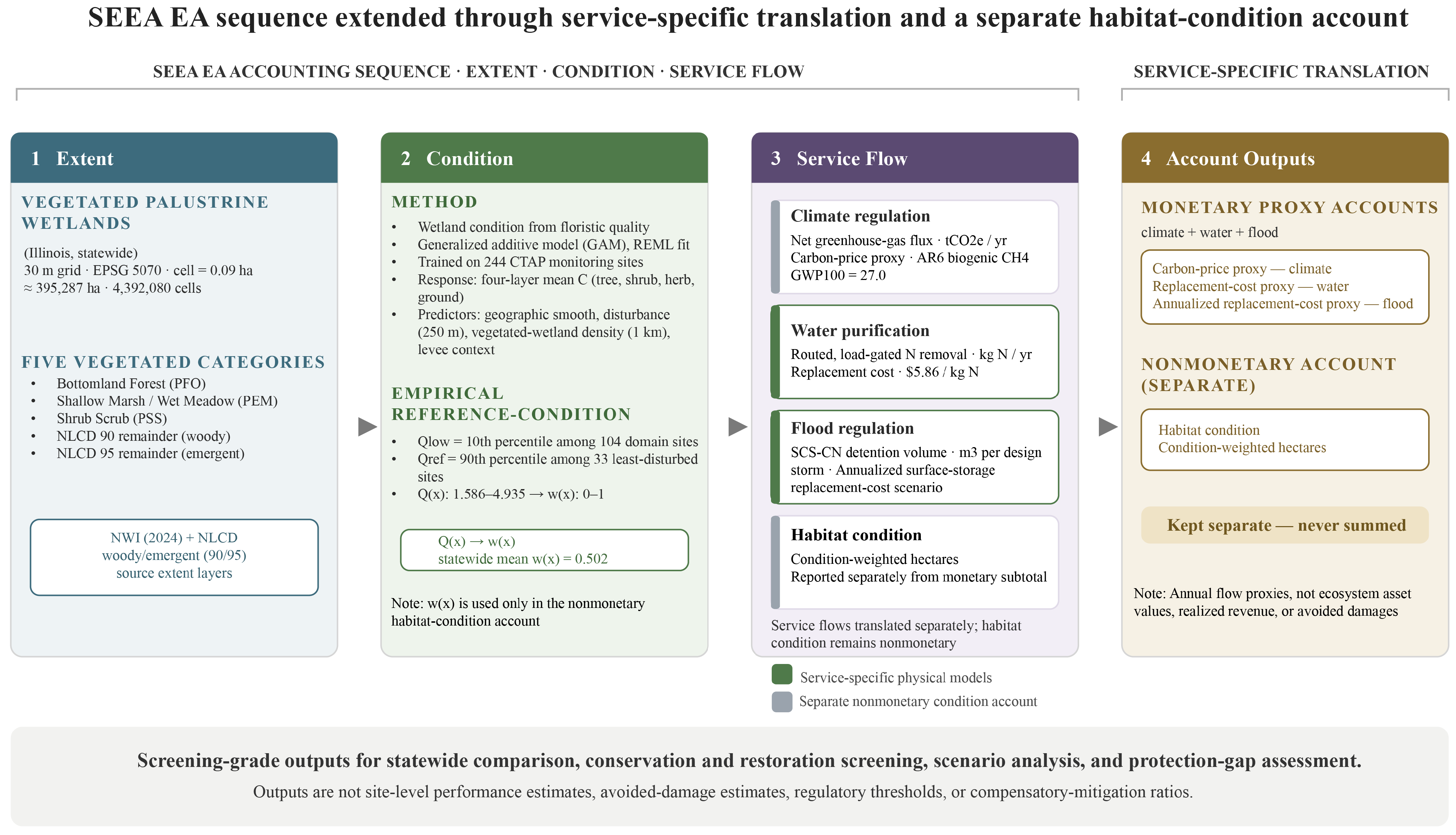
This paper develops an ecosystem accounting framework for Illinois palustrine wetlands that links ecosystem extent, floristic condition, service-specific physical flows, monetary proxy accounts, and protection-gap screening. The framework follows the SEEA EA sequence of extent, condition, and service flow, and extends it through service-specific monetary translation and a separate nonmonetary habitat-condition account. Wetland condition is derived from floristic quality and expressed through the scalar $w\left(x\right)$. The scalar is used only to construct the habitat-condition account and is not applied to the climate regulation, water purification, or flood regulation monetary accounts.

Three monetary service accounts are developed for climate regulation, water purification, and flood regulation, and ecological condition is reported separately through the habitat-condition account. All accounts are mapped on a statewide 30 m × 30 m grid. The floristic-condition layer allows wetlands within the same mapped category to differ in ecological condition without assuming that the same condition scalar controls all service flows. Climate regulation is reported as a carbon-price proxy, water purification as a nitrogen-removal replacement-cost proxy, and flood regulation as an annualized surface-storage replacement-cost scenario. The habitat-condition account is reported in condition-weighted hectares and is not monetized or added to the monetary subtotal.

The main contribution of this paper is an ecosystem accounting framework that translates fragmented wetland evidence into planning-ready, spatially explicit information. Rather than applying a single ecological-condition multiplier across all services, the framework uses service-specific physical models for climate regulation, water purification, and flood regulation, while reporting floristic condition separately through a nonmonetary habitat-condition account. This structure preserves differences among ecological condition, physical service flows, and monetary proxy types while aligning them on a common statewide 30 m × 30 m grid. The resulting accounts support spatial screening, conservation targeting, restoration prioritization, and protection-gap analysis. The analysis also shows that a substantial share of the classified wetland extent and habitat-condition account occurs in wetlands classified as unprotected [11]. By integrating ecological condition, service-specific physical flows, monetary proxy accounts, and institutional protection status, the framework also provides a practical sustainability tool for monitoring wetland assets, evaluating land-use tradeoffs, and supporting conservation and restoration decisions.

The rest of this paper is organized as follows. Section 2 reviews ecosystem accounting, ecological condition, and the biophysical and valuation evidence underlying the three monetary service accounts and the nonmonetary habitat-condition account. Section 3 describes the account structure, wetland extent and condition modeling, service-specific physical and monetary methods, and protection-gap overlay. Section 4 reports the condition surface, statewide monetary proxy accounts, differences among wetland categories, the habitat-condition account, and protection-gap results. Section 5 discusses planning implications, methodological limitations, uncertainty, and priorities for future refinement.

2. Literature Review

Wetlands are widely recognized as multifunctional ecosystems that provide climate regulation through carbon storage and sequestration [17], water quality improvement through nutrient retention and pollutant removal [18,19], flood attenuation through runoff buffering and temporary water storage [20,21], and habitat support for biodiversity [1,4]. Despite this broad recognition, translating ecosystem service knowledge into planning usable information remains challenging because the type, production, and communication of ecosystem service information must be adapted to specific planning contexts [8]. For wetland planning, this creates a need to organize evidence in spatially explicit forms that can compare multiple wetland types and service categories simultaneously.

Landscape planning scholarship has long recognized the gap between ecological knowledge and actionable planning information. Nassauer and Opdam [22] argued that landscape ecology has been more effective at generating knowledge than at transferring it into societal use, and proposed design as a common ground for linking pattern and process science to decision making. Termorshuizen and Opdam [23] identified two requirements for landscape ecological research to support planning practice: it must include a valuation component, and it must be suitable for collaborative, spatially explicit decision making. Wetland ecosystem services illustrate this challenge clearly. The question is not whether wetlands provide benefits, but how those benefits can be translated into spatial information for screening, comparison, and prioritization.

2.1. Accounting Structure and Value Concepts

The ecosystem accounting literature provides a structured approach for organizing ecosystem information across physical and monetary dimensions. The System of Environmental Economic Accounting Ecosystem Accounting framework distinguishes ecosystem extent, condition, and service flow accounts, and provides a basis for linking ecological change to economic and planning information [24] (United Nations [25]). Earlier accounting studies also emphasize that ecosystem service valuation must remain consistent with national accounting principles, especially when monetary estimates are intended to be comparable across services or incorporated into broader environmental economic accounts [26,27]. Warnell et al. [28] provide a closely related U.S. precedent through their compilation of ecosystem extent, condition, and service accounts across ten southeastern states. Building on this regional accounting approach, the present study focuses on Illinois wetlands and on translating multiple accounts into a common spatial structure for planning and protection-gap screening.

A central issue in this literature is the distinction between exchange values and welfare-based values. Exchange values are designed to align with the System of National Accounts and exclude consumer surplus, while welfare-based values capture broader changes in human well-being that may include consumer surplus [25,26,27]. This distinction is especially important in ecosystem service studies because monetary estimates are often derived from different valuation logics, including market prices, replacement costs, avoided damages, policy prices, and stated-preference methods. When estimates with different valuation bases are aggregated without clarification, the resulting totals can be difficult to interpret or compare across studies [7,29].

Wetland valuation studies illustrate this challenge clearly. Meta-analyses show that wetlands provide a wide range of valued services, including water-quality improvement, flood regulation, recreation, habitat provision, and biodiversity support, but estimated values vary by wetland type, service category, valuation method, and geographic context [7,30]. Biodiversity and habitat condition are particularly difficult to represent through a physical-quantity-times-price approach. Monetary estimates often rely on nonmarket valuation methods and can be sensitive to beneficiary population, elicitation format, geographic context, and the definition of the conservation outcome.

2.2. Ecological Condition and Ecosystem Service Delivery

Floristic quality assessment, and the mean coefficient of conservatism in particular, has been widely used as an indicator of ecological integrity in Midwestern plant communities and wetland landscapes [31]. Matthews [32] evaluated the floristic quality index in Illinois wetlands and showed that it can provide useful information on wetland community quality, while also finding that values vary with wetland area, community type, and survey timing. Spyreas [33] identified mean C as one of the most commonly applied and influential indicators of site condition across regional ecological assessments. Because mean C reflects the composition of species with differing tolerances to disturbance, it serves as a useful indicator of ecological quality, although its interpretation should be considered alongside other ecological characteristics and assessment measures.

The broader ecological literature links vegetation integrity to ecosystem functioning. Wetland vegetation influences nutrient processing, hydrologic performance, habitat structure, and biogeochemical processes [34]. Zedler [35] showed that wetland loss and degradation in agricultural watersheds can reduce flood abatement, water quality improvement, and biodiversity support. Together, these studies support ecological condition as an important dimension of wetland assessment, while also showing that floristic condition should not be treated as a complete or universally calibrated measure of individual ecosystem-service performance.

Benefit-transfer studies reinforce the importance of ecological and contextual correspondence. Benefit transfer applies estimates from prior studies when primary site-specific valuation is not feasible because of time, cost, or data constraints [36,37]. Its reliability depends on the similarity between the original study context and the policy site. Transfer error can arise when transferred estimates ignore differences in ecosystem type, landscape context, service supply, beneficiary population, income, scarcity, or ecological condition [7,29,37]. Johnston et al. [37] identified site quality as an important determinant of transfer accuracy and noted that ignoring ecological differences between study and policy sites can introduce systematic bias.

2.3. Wetland Ecosystem Services: Biophysical Evidence and Valuation Concepts

The literature on wetland ecosystem services shows that different services are measured through different biophysical indicators and valued through different monetary concepts. Climate regulation illustrates this issue clearly. Wetlands are frequently described as carbon sinks, but this characterization can be incomplete because net greenhouse gas balance depends on both carbon sequestration in soil and biomass and methane emissions from anaerobic decomposition [2]. Villa and Bernal [38] found that freshwater wetland sequestration rates vary substantially with vegetation class, hydrology, and geographic setting. Pang and Deal [39] applied this evidence base to Illinois wetland types and documented a clear north south gradient in sequestration capacity, with bottomland forests functioning as the strongest sinks and open water systems acting as net sources. Methane has a substantially higher 100-year global warming potential than CO₂, with the applicable value depending on the IPCC assessment framework. Pulliam [40] reported a methane flux of about 17 g of methane-carbon per square meter per year (g CH₄-C m⁻² yr⁻¹) for bottomland hardwood systems. Converted to a methane mass basis using the CH₄ to C molecular weight ratio of 16/12, this corresponds to roughly 23 g CH₄ m⁻² yr⁻¹ [2].

Carbon valuation also demonstrates the importance of distinguishing value concepts. Compliance-market prices, including linked California–Québec auction settlement prices and Regional Greenhouse Gas Initiative auction prices, represent observed transactions within regulated carbon markets [41,42]. These prices differ from the social cost of carbon, which estimates the marginal global welfare damages associated with an additional ton of CO₂ emissions (EPA [43]). Shadow prices occupy a third category because they can be constructed to reflect policy targets or mitigation pathways rather than observed market transactions (Carbon Pricing Leadership Coalition [44]). For ecosystem accounting, market prices, policy prices, and welfare based damage estimates do not represent the same value concept and must be interpreted according to the accounting purpose for which they are used.

Water purification presents a different translation challenge because the physical evidence is often site specific while monetary evidence is usually drawn from engineered treatment or regulatory cost contexts. Kovacic et al. [3] monitored three constructed wetlands in east central Illinois, approximately 1.4 hectares (ha) combined, receiving agricultural tile drainage, and measured removal of roughly 400 kg of nitrogen per hectare per year (kg N ha⁻¹ yr⁻¹). Crumpton et al. [45] reported higher nitrogen removal rates, approximately 1500 kg N ha⁻¹ yr⁻¹, across 26 restored Iowa wetlands receiving higher nitrogen loads. These studies show that wetlands can remove substantial nitrogen loads from agricultural runoff, while also demonstrating that removal rates vary with loading conditions, system design, and site context.

Replacement cost valuation is commonly used when an ecosystem service can be compared with an engineered or institutional substitute. In the case of nitrogen removal, physical estimates of wetland nutrient retention can be paired with treatment cost benchmarks from wastewater or nutrient removal technologies. The USEPA Municipal Nutrient Removal Technologies Reference Document reports unit costs for total nitrogen removal across case study facilities, ranging from USD 0.63 to USD 4.86 per pound, or approximately USD 1.39 to USD 10.71 per kilogram (kg) [46]. In valuation terms, replacement cost estimates do not measure the full welfare value of improved water quality. Instead, they approximate the cost of providing a comparable service through an alternative technological or management pathway rather than direct willingness to pay.

Flood regulation adds a further layer of complexity because wetland effects on flooding are highly dependent on hydrologic setting, landscape position, soil saturation, storage capacity, and event timing. Bullock and Acreman [47] reviewed the hydrological role of wetlands and found that downstream flood effects vary substantially by wetland type and antecedent moisture conditions. Some wetlands can reduce downstream flood peaks by storing and slowing runoff, while wetlands that are already saturated may provide limited additional detention during large events. This hydrological variability also affects valuation because flood regulation estimates depend on the flood process being measured, the exposed assets or populations considered, and the counterfactual used for comparison. Flood regulation values may therefore reflect reduced flood damages, the cost of substitute infrastructure, property market effects, or stated willingness to pay for risk reduction. These approaches capture different aspects of value and are difficult to compare without clarifying the value concept each estimate represents.

Habitat and biodiversity differ from carbon storage, nitrogen removal, and flood regulation because they are less readily represented through a physical-quantity-times-price pathway. Biodiversity includes ecological composition, integrity, rarity, habitat structure, and conservation outcomes that are difficult to reduce to a single biophysical unit. Monetary valuation has therefore commonly relied on nonmarket methods, including contingent valuation and choice experiments, which estimate willingness to pay or willingness to accept for specified conservation outcomes. However, such estimates can vary substantially with beneficiary population, elicitation format, geographic context, ecological scarcity, wetland type, and the definition of the outcome being valued [7,30,48]. This variability limits the direct transferability and comparability of monetary biodiversity estimates across locations and planning contexts.

2.4. A Persistent Translation Gap

Wetland science has generated many valid metrics for carbon flux, nutrient removal, hydrologic regulation, habitat support, and ecological condition, but these metrics are rarely assembled into a common structure that can support planning decisions. Service studies often rely on generalized per-hectare transfers that do not fully represent spatial variation in loading, hydrologic setting, wetland type, or ecological context, while condition indicators are commonly developed and reported through separate assessment systems. In addition, these studies often focus on one service at a time, while drawing on different value concepts, including exchange values, replacement costs, policy prices, avoided damages, and welfare-based willingness-to-pay estimates.

Recent Illinois policy developments add practical urgency to this translation problem. Peterson et al. [11] estimated that, following the Sackett v. EPA decision [10], a substantial share of Illinois wetlands may lack federal protection, with implications for ecosystem service delivery and community flood vulnerability. Their protection-status classifications provide an important spatial foundation for understanding wetland vulnerability. However, the broader literature still lacks a consistent spatial structure for aligning protection status, ecological condition, service-specific physical flows, and monetary valuation while preserving the conceptual distinctions among them. The gap is therefore not an absence of wetland evidence, but the lack of spatially explicit and conceptually consistent information that can support screening, comparison, and prioritization in planning practice.

3. Materials and Methods

The proposed framework operationalizes the SEEA EA accounting structure through a four-step translation. Section 3.1 presents the translation framework and account structure. Section 3.2 develops the 30 m × 30 m vegetated-wetland extent account and the generalized additive model (GAM)-derived condition surface. Section 3.3 specifies the service-specific physical and monetary methods for climate regulation, water purification, and flood regulation, together with a separate nonmonetary habitat-condition account. Section 3.4 describes the account outputs and protection-gap analysis.

3.1. Translation Framework and Account Structure

This study develops a four-step translation that converts ecological evidence into planning-ready spatial metrics. The framework follows the SEEA EA sequence of ecosystem extent, condition, and service flow and extends it through service-specific monetary translation and a separate nonmonetary habitat-condition account (Figure 1). The contribution lies in the translation structure rather than in the development of new valuation coefficients. The resulting outputs are intended to support statewide screening, conservation targeting, restoration prioritization, and protection-gap analysis.

All spatial operations were performed on a 30 m × 30 m raster grid aligned to the 2024 National Land Cover Database (NLCD) [49] in the NAD83/Conus Albers projection (EPSG:5070). All analyses were conducted in R version 4.5.2 using the terra version 1.8-60, sf version 1.0-20, mgcv version 1.9-3, and blockCV version 3.2.0 packages.

The framework produces screening-grade metrics intended for statewide spatial prioritization, conservation and restoration screening, protection-gap analysis, and comparison across wetland categories and accounts. The outputs are not intended as site-level estimates of ecological performance or avoided damages, regulatory performance thresholds, or compensatory-mitigation equivalency ratios.

3.2. Extent and Condition Accounts

The canonical vegetated-wetland raster was derived by intersecting U.S. Fish and Wildlife Service National Wetlands Inventory (NWI) polygons from the 2024 release [50] with the 2024 NLCD woody wetlands (class 90) and emergent herbaceous wetlands (class 95) [49]. Five mutually exclusive wetland categories were defined:

• Bottomland Forest, NWI Cowardin class PFO (Palustrine Forested) within NLCD class 90;
• Shallow Marsh and Wet Meadow, NWI class PEM (Palustrine Emergent) within NLCD class 95;
• Shrub-Scrub Wetlands, NWI class PSS (Palustrine Scrub-Shrub) within NLCD class 90;
• NLCD 90 Remainder, consisting of NLCD class 90 cells without a corresponding NWI vegetation class;
• NLCD 95 Remainder, consisting of NLCD class 95 cells without a corresponding NWI vegetation class.

The resulting vegetated-wetland extent account contains 4,392,080 cells, equivalent to 395,287 ha. Cell counts and raster alignment were checked across downstream scripts using reproducibility guards to prevent unintended changes in the canonical analysis mask.

The condition account uses the site-level four-layer mean coefficient of conservatism (fourLayerMeanC), which integrates tree, shrub, herbaceous, and ground-layer observations. Species-level coefficients of conservatism follow the Illinois assignments of Taft et al. [31], ranging from $C=0$ for disturbance-tolerant generalists to $C=10$ for conservative species associated with least-disturbed ecological conditions. For each site, the response variable was calculated as the temporal mean across all available survey visits from 1997 to 2022. The modeling dataset included $N=244$ Critical Trends Assessment Program (CTAP) palustrine wetland monitoring sites identified by CTAP Habitat == "W".

The floristic response therefore represents a multiyear site average, whereas the surrounding land-cover predictors were derived from the 2024 NLCD and represent a contemporary landscape snapshot. The analysis does not reconstruct changes in surrounding disturbance over the 1997–2022 monitoring period, and associations with these predictors are not interpreted as time-matched causal effects.

A generalized additive model (GAM) was fitted by restricted maximum likelihood (REML) using the mgcv package (version 1.9-3) [51], with the specification

$$\begin{array}{ccc}\hfill \mathtt{fourLayerMeanC}& \sim & \mathtt{s}(\mathtt{lon}\_\mathtt{proj}, \mathtt{lat}\_\mathtt{proj}, \mathtt{bs}="\mathtt{tp}", \mathtt{k}=\mathtt{29})\hfill \\ & & +\mathtt{s}(\mathtt{disturbance}\_\mathtt{250}\mathtt{m}, \mathtt{bs}="\mathtt{ts}", \mathtt{k}=\mathtt{10})\hfill \\ & & +\mathtt{s}(\mathtt{wetdens}\_\mathtt{veg}\_\mathtt{1}\mathtt{km}, \mathtt{bs}="\mathtt{ts}", \mathtt{k}=\mathtt{10})\hfill \\ & & +\mathtt{levee}\_\mathtt{binary}.\hfill \end{array}$$

(1)

Landscape disturbance and levee context formed the base model. Their retention was confirmed using drop-one tests, in which removing either term reduced spatially cross-validated predictive performance and increased AIC. The remaining seven covariates were evaluated one at a time as additions to the base model. An add-one candidate was retained only if it increased spatially cross-validated $R^2$ by more than 0.005, reduced AIC by more than 2, and did not exceed the collinearity threshold of $\left|r\right|=0.7$ with a retained covariate. Vegetated-wetland density within 1 km met all three criteria and was added to the final model. The other candidates were excluded because they did not improve out-of-sample performance, were effectively uninformative, or were collinear with a retained covariate. In addition to the two-dimensional geographic smooth, nine candidate covariates were considered: landscape disturbance within 250 m, levee context, vegetated-wetland density within 1 km, available water capacity, agricultural cover within 500 m, forest cover within 2 km, topographic wetness index, distance to the nearest flowline, and NWI water regime. Landscape disturbance and levee context formed the base model. The remaining seven covariates were evaluated individually as additions to that base model. Predictor-screening results, including changes in spatially cross-validated $R^2$, AIC, effective degrees of freedom, and collinearity, are reported in Table S1.

Predictive performance was evaluated using a seeded 50-km, five-fold spatial block cross-validation design generated with blockCV (selection = "random", 100 iterations, seed 42). Performance was reported using pooled and mean-fold cross-validated $R^2$, RMSE, and MAE. The final model produced a pooled spatial-CV $R^2$ of 0.261, a mean-fold $R^2$ of 0.251, an RMSE of 0.727, and an MAE of 0.572. Basis dimensions were checked using k.check, and residual spatial autocorrelation was evaluated using Moran’s I.

The two-dimensional geographic smooth represents broad spatial structure in floristic condition that is not explained by the measured landscape predictors. Landscape disturbance within 250 m was calculated as the proportion of developed land (NLCD classes 21–24) and agricultural land (classes 81–82) within a circular focal window and was used as a proxy for surrounding anthropogenic disturbance. Vegetated-wetland density within 1 km was calculated as the proportion of mapped vegetated-wetland cover within the surrounding neighborhood. Levee context was represented by a binary variable derived from the U.S. Army Corps of Engineers National Levee Database, indicating whether a site occurred inside or outside a mapped leveed area. These predictors are interpreted as screening-level spatial correlates of floristic condition rather than direct causal measures of runoff, hydrologic connectivity, or ecological degradation.

The fitted GAM was applied spatially to generate a continuous condition surface $Q\left(x\right)$ at 30 m resolution across all vegetated-wetland cells. Predicted values ranged from 1.586 to 4.935. These values represent the mapped range of model-predicted floristic condition across Illinois vegetated wetlands rather than the full theoretical Mean C scale of 0 to 10. $Q\left(x\right)$ was rescaled to a condition scalar $w\left(x\right)\in [0,1]$ using a two-anchor linear transformation:

$$w\left(x\right)=min\left(1,max\left(0,{\displaystyle \frac{Q\left(x\right)-Q_{\mathrm{low}}}{Q_{\mathrm{ref}}-Q_{\mathrm{low}}}}\right)\right).$$

(2)

The primary reference-condition definition was based on the 104 CTAP sites located within the mapped vegetated-wetland prediction domain. A least-disturbed subset was defined a priori as sites whose 250-m disturbance proportion fell within the lowest tercile of the domain distribution and that were located outside mapped levees. This screening yielded 33 least-disturbed sites. The lower anchor, $Q_{\mathrm{low}}=1.752$, was defined as the 10th percentile of observed four-layer Mean C across the 104 domain sites, and the reference anchor, $Q_{\mathrm{ref}}=4.311$, was defined as the 90th percentile of observed four-layer Mean C within the 33-site least-disturbed subset. Predicted values at or above $Q_{\mathrm{ref}}$ were clamped to $w\left(x\right)=1$, while values at or below $Q_{\mathrm{low}}$ were clamped to $w\left(x\right)=0$.

The condition scalar $w\left(x\right)$ is a screening-level indicator of relative habitat condition derived from floristic quality. It is applied only in calculating condition-weighted area for the nonmonetary habitat-condition account and is not used to scale the climate-regulation, water-purification, or flood-regulation accounts, which are estimated using service-specific physical methods. Floristic integrity is used here as a vegetation-based proxy for habitat condition [34,35]. However, $w\left(x\right)$ is not an empirically calibrated causal coefficient linking floristic quality to the performance of any individual ecosystem service. This limitation is discussed further in Section 5.

3.3. Service Flow and Monetary Accounts

The framework includes three monetary service accounts—climate regulation, water purification, and flood regulation—and one separate nonmonetary habitat-condition account. For each monetary account, the physical service flow was estimated first and then translated using a service-specific carbon-price or replacement-cost proxy. The habitat-condition account is reported in condition-weighted hectares and is not monetized or added to the monetary subtotal. This structure preserves the distinctions among physical service flows, monetary proxies, and ecological condition.

Climate Regulation. Net greenhouse-gas flux was estimated for each 30 m × 30 m wetland cell as carbon sequestration minus methane emissions, expressed in metric tons of carbon dioxide equivalent per year (tCO₂e yr⁻¹). Literature-informed carbon-sequestration rates were assigned by wetland category using Villa and Bernal [38] and Bridgham et al. [2]. Methane base rates were assigned by wetland category and subsequently adjusted using an inundation index derived from the NWI Cowardin water-regime classification (

Table 1. Literature-based carbon-sequestration and methane-rate assumptions by wetland category.

Category	Sequestration Rate	CH4 Base Rate	Source or Assignment Basis
	(tCO2e acre−1 yr−1)	(g CH4 m−2 yr−1)
Bottomland Forest	2.70	23.0	Pulliam [40]; Bridgham et al. [2]
Shallow Marsh/Wet Meadow	1.53	50.0	Altor and Mitsch [52]
Shrub-Scrub Wetlands	1.48	12.4	Werner et al. [53]
NLCD 90 Remainder (Woody)	2.10	23.0	Literature-informed woody-wetland proxy; methane rate assigned from Bottomland Forest
NLCD 95 Remainder (Emergent)	1.10	50.0	Literature-informed emergent-wetland proxy; methane rate assigned from Shallow Marsh/Wet Meadow

).

Methane base rates were converted to a CH₄ mass basis where necessary. For each wetland cell, the category-specific methane base rate was multiplied by an inundation index assigned from the NWI Cowardin water-regime classification (

Table 2. Inundation-index assumptions by NWI Cowardin water regime.

Water Regime	Cowardin Letters	Inundation Index
Permanent	H, G, F	1.00
Seasonal	E, D, C	0.60
Intermittent	J, K	0.35
Temporary	A, B	0.25
Unknown (no NWI regime)	—	0.50

). Methane emissions were then converted to CO₂ equivalent using the IPCC AR6 100-year global warming potential of 27.0 for biogenic CH₄. The IPCC AR4 value of 25 was evaluated separately as a sensitivity analysis. Cells in the NLCD 90 and NLCD 95 Remainder categories lack NWI water-regime attribution and were therefore assigned an unknown-regime inundation index of 0.5.

Because Illinois does not operate a compliance carbon market, net greenhouse-gas flux was translated using transferred carbon-price proxies rather than the social cost of carbon. The central scenario value of USD 28 per tCO₂e was derived from recent linked California–Québec cap-and-trade auction prices and was used as an external policy-price benchmark rather than as an Illinois market price. The low scenario value of USD 20 per tCO₂e was based on a Regional Greenhouse Gas Initiative auction benchmark, while the high scenario value of USD 50 per tCO₂e was drawn from the lower end of a World Bank carbon-price trajectory. The latter is a shadow-price benchmark rather than an observed market transaction. These transferred values define policy-price scenarios and should not be interpreted as estimates of the social cost of carbon or as realized market revenue from Illinois wetlands (

Table 3. Carbon-price scenarios used to translate net climate-regulation flux.

Scenario	Price ($/tCO2e)	Source or Basis
Low	$20	RGGI auction benchmark [42]
Central	$28	Linked California–Québec joint-auction benchmark [41]
High	$50	Lower end of the World Bank 2030 shadow-price trajectory [54]

).

Water Purification (N Removal). Nitrogen removal was estimated on the National Hydrography Dataset Plus High Resolution (NHDPlus HR) network rather than by applying a uniform per-hectare removal rate to all wetland cells. Nitrogen source loads were assigned using export coefficients of 30 kg N ha⁻¹ yr⁻¹ for cultivated crops and 5 kg N ha⁻¹ yr⁻¹ for pasture and hay. These coefficients are consistent with values reported for tile-drained row-crop systems in Illinois and published land-use export-coefficient syntheses [55,56,57]. Together, they produced a modeled statewide source load of 0.279 Tg N yr⁻¹.

Source loads were routed downstream through connected NHDPlus HR flowlines. For wetland reach i, nitrogen removal was constrained by both an areal removal capacity and the load delivered to the reach:

$$R_i=min\left(400A_i,\rho L_{i,\mathrm{in}}\right),$$

(3)

where $R_i$ is annual nitrogen removal in kg N yr⁻¹, $A_i$ is wetland area in hectares, $L_{i,\mathrm{in}}$ is the incoming nitrogen load, and $\rho$ is the retained fraction of the incoming load. The central value $\rho =0.4$ is close to the reported meta-analytic median total-nitrogen removal efficiency of 37% and lies within its 95% confidence interval of 29–44% [58]. The areal cap of 400 kg N ha⁻¹ yr⁻¹ is below the reported median areal total-nitrogen removal rate of approximately 930 kg N ha⁻¹ yr⁻¹ across the wetlands included in the meta-analysis and therefore provides a conservative upper constraint on modeled removal.

Of the modeled Illinois source load, 99.54% was matched to the assembled routing network. A mass-balance check confirmed conservation of the matched load through the routing procedure. The remaining 0.46% occurred in catchments without a matching FlowlineVAA record and was reported separately rather than treated as routing loss. Under the central retention fraction $\rho =0.4$, statewide routed nitrogen removal was 57.7 million kg N yr⁻¹. Because no in-stream attenuation was applied, this estimate represents an upper-delivery screening scenario.

Removed nitrogen was valued using a central municipal biological nutrient-removal replacement cost of USD 5.86 per kg N [46]. The value assigned to wetland cell x was

$$V_{\mathrm{wp}}\left(x\right)=P_{\mathrm{N}}{M}_{\mathrm{rem}}\left(x\right),$$

(4)

where $P_{\mathrm{N}}=\$5.86{\mathrm{kg}}^{-1}\mathrm{N}$ and $M_{\mathrm{rem}}\left(x\right)$ is the routed, load-gated nitrogen removal allocated to cell x. Floristic condition does not enter this estimate. The central statewide water-purification replacement-cost proxy is USD 338.0 million yr⁻¹. Holding the export coefficients constant and varying $\rho$ from 0.2 to 0.6 changes the statewide estimate from USD 313.6 million to USD 350.3 million yr⁻¹.

Flood Regulation. Flood regulation was estimated as an annualized surface-storage replacement-cost scenario based on modeled runoff reduction, with no floristic-condition adjustment and no event-frequency multiplier. Runoff depth was computed using the SCS Curve Number method described in Technical Release 55 [59].

$$Q=\left\{\begin{array}{cc}{\displaystyle \frac{{(P-I_a)}^2}{P-I_a+S}},\hfill & P>I_a,\hfill \\ 0,\hfill & P\le I_a,\hfill \end{array}\right.S={\displaystyle \frac{\mathrm{25,400}}{\mathrm{CN}}}-254,I_a=0.2S.$$

(5)

where Q, P, S, and $I_a$ are expressed in millimeters. For each 30 m × 30 m cell, runoff reduction relative to the specified counterfactual was calculated as $\Delta Q=Q_{\mathrm{counterfactual}}-Q_{\mathrm{present}}$. Negative values were set to zero. Retained volume was then calculated as $\Delta V=\Delta Q\times 900{\mathrm{m}}^2/1000$, expressed in m³ per cell.

Curve numbers were assigned by NLCD land-cover class and hydrologic soil group under antecedent moisture condition II (

Table 4. Curve numbers by NLCD land-cover class and hydrologic soil group under antecedent moisture condition II.

NLCD Class	Land Cover	A	B	C	D
11	Open Water	100	100	100	100
21	Developed, Open Space	49	69	79	84
22	Developed, Low Intensity	61	75	83	87
23	Developed, Medium Intensity	77	85	90	92
24	Developed, High Intensity	89	92	94	95
31	Barren Land	77	86	91	94
41/42/43	Deciduous, Evergreen, and Mixed Forest	36	60	73	79
51/52	Dwarf Scrub and Shrub-Scrub	48	67	77	83
71/72/73/74	Grassland, Sedge, Lichens, and Moss	49	69	79	84
81	Pasture/Hay	49	69	79	84
82	Cultivated Crops	67	78	85	89
90	Woody Wetlands (present condition)	30	55	70	77
95	Emergent Herbaceous Wetlands (present condition)	30	58	71	78

Notes. Values represent antecedent moisture condition II. Upland land-cover curve numbers follow TR-55 tables for the corresponding cover conditions and hydrologic soil groups. Wetland curve numbers follow the wetland values used in the analysis. Hydrologic soil groups A–D indicate progressively lower infiltration capacity and greater runoff potential.

). Hydrologic soil group was obtained from the dominant gSSURGO component, with dual classes A/D, B/D, and C/D assigned to group D under wet conditions. The counterfactual represents simplified agricultural-conversion pathways informed by documented wetland losses to agricultural land uses [60,61]. Woody wetlands were represented as pasture/hay and emergent wetlands as cultivated crops for scenario construction; these assignments are modeling assumptions rather than empirically observed cell-level transitions.

Antecedent-moisture adjustments were applied only to present wetland cells using NWI Cowardin water-regime classes, while counterfactual land-cover cells remained under condition II. Condition I and condition III curve numbers were derived from condition II values as

$${\mathrm{CN}}_{\mathrm{I}}={\displaystyle \frac{4.2{\mathrm{CN}}_{\mathrm{II}}}{10-0.058{\mathrm{CN}}_{\mathrm{II}}}},{\mathrm{CN}}_{\mathrm{III}}={\displaystyle \frac{23{\mathrm{CN}}_{\mathrm{II}}}{10+0.13{\mathrm{CN}}_{\mathrm{II}}}}.$$

Permanent water regimes were assigned to condition III, seasonal regimes to condition II, and temporary regimes to condition I. Because the condition I transformation produced a small tail of adjusted values below the empirical range represented in the wetland curve-number lookup table, present-wetland curve numbers were floored at 30, the minimum tabulated wetland curve number used in the analysis, and capped at 100.

A sensitivity check showed that the curve-number floor left the annualized replacement-cost estimates for the 5-year and central 10-year scenarios unchanged. It reduced the 25-year high-scenario estimate by 0.41%, from USD 2435.0 million to USD 2425.1 million yr⁻¹. Cells with $\Delta Q<0$, primarily permanently saturated wetlands whose adjusted present-condition curve number exceeded that of the upland counterfactual, were assigned $\Delta Q=0$ because they provided no modeled additional detention under the specified storm scenario.

The 5-, 10-, and 25-year design-storm scenarios used fixed statewide 24-hour rainfall depths of 95, 114, and 135 mm, respectively. These values were treated as screening assumptions informed by Illinois precipitation-frequency guidance, including NOAA Atlas 14, Volume 2 [62], rather than as location-specific precipitation estimates. Spatial variation in precipitation frequency across Illinois was not modeled, and each storm was evaluated as a separate scenario rather than combined probabilistically. Because wet-detention construction cost represents a capital expenditure rather than an annual service flow, it was annualized using a capital recovery factor:

$$\mathrm{CRF}={\displaystyle \frac{i{(1+i)}^n}{{(1+i)}^n-1}},c_{\mathrm{ann}}=P_{\mathrm{cap}}\left(\mathrm{CRF}+m\right).$$

(6)

where $P_{\mathrm{cap}}$ is the installed capital cost per ${\mathrm{m}}^3$, i is the discount rate, n is infrastructure service life in years, and m is annual operation and maintenance expressed as a fraction of installed capital. The annualized replacement cost assigned to cell x was $V_{\mathrm{flood}}\left(x\right)=c_{\mathrm{ann}}\Delta V\left(x\right)$.

The base construction-cost range of $17.50–$35.00 per m³ corresponds to the U.S. EPA wet-detention [63] estimate of USD 0.50–USD 1.00 per ft³, reported in 1997 dollars. The central value of USD 26.25 per m³ is the midpoint of this range. Costs were converted to 2025 U.S. dollars using ENR 20-city Construction Cost Index annual averages of 5826 for 1997 and 13,901 for 2025, giving an escalation factor of 2.386. A central soft cost multiplier of 1.25 produced an installed capital cost of $26.25\times 2.386\times 1.25=\$78.29$ per m³. Annual operation and maintenance was represented as 3–5% of installed capital under the scenario assumptions.

Because routing from cell-level retained volume to downstream flood stage was not validated, this account is reported as an annualized surface-storage replacement-cost scenario. It represents the modeled cost of constructing equivalent detention capacity and is not an estimate of avoided flood damages. Cell-level runoff reduction is therefore not equated with downstream stage or damage reduction. Low, central, and high scenarios jointly vary storm depth, construction cost, soft costs, service life, discount rate, and operation and maintenance and should be interpreted as scenario bounds rather than confidence intervals.

3.4. Account Outputs and Protection-Gap Analysis

Outputs were summarized by wetland category and for the statewide vegetated-wetland extent. For each monetary account, we reported the underlying physical quantity, the monetary proxy per cell, and the statewide and category-level annual monetary totals. Climate regulation was reported in tCO₂e yr⁻¹, water purification in kg N yr⁻¹, and flood regulation as modeled detention volume in m³ under each design-storm scenario. Flood detention is an event-based physical quantity; only its replacement-cost proxy was annualized. Habitat condition was reported separately in condition-weighted hectares.

The outputs are intended for cross-account screening within planning workflows and should not be interpreted as strictly equivalent measures of benefit. Climate regulation is translated using transferred carbon-price scenarios, whereas water purification and flood regulation are translated using replacement-cost scenarios. These monetary proxies are not estimates of realized revenue, observed avoided expenditure, or net social benefit. The nonmonetary habitat-condition account is not monetized and is not added to the monetary subtotal. All monetary outputs are annual flow proxies rather than ecosystem-asset stock values.

Per-acre monetary values were calculated by dividing each statewide annual monetary total by the full vegetated-wetland extent of 4,392,080 cells. At $900{\mathrm{m}}^2$ per cell, this corresponds to 395,287 ha, or approximately 976,800 acres. This statewide denominator differs from the denominator used in the protection-gap analysis, which includes only cells assigned a protection tier by Peterson et al. [11].

For broad contextual comparison only, the statewide monetary proxy subtotal was expressed on a per-acre basis and compared with reported Illinois cropland cash rents. The statewide average cropland cash rent reported for Illinois in 2025 was USD 264 per acre [64], while projected rents by land quality ranged from approximately USD 198 per acre for fair-quality land to USD 381 per acre for excellent-quality land [65]. Cash rent represents a realized private return to land, whereas the wetland estimates are carbon-price and replacement-cost proxies for public regulating services. The measures are not directly equivalent. Wetland and cropland parcels were not spatially matched, and drainage, conversion, production, transaction, and opportunity costs were not included. The habitat-condition account was excluded from this comparison.

Protection-gap screening was conducted by intersecting the canonical vegetated-wetland raster and habitat-condition surface with the four-tier protection classification of Peterson et al. [11]. Wetland extent and condition-weighted habitat area were summarized separately for each protection tier and for cells outside the classified coverage. Unclassified cells were retained in statewide totals but excluded from percentage calculations whose denominator was restricted to classified wetlands. The analysis identifies where mapped wetland extent and modeled habitat condition coincide with lower institutional protection; it does not determine legal jurisdiction, site-specific regulatory status, or conservation priority by itself.

The low, central, and high assumptions used in the monetary accounts are summarized in

Table 5. Central parameters and scenario assumptions used in the wetland-account translation framework.

Account	Parameter	Low	Central	High	Unit	Source or Basis
Climate regulation	Carbon price	20	28	50	$/tCO2e	RGGI auction benchmark [42]; California–Québec joint-auction benchmark [41]; World Bank shadow-price trajectory [54]
Climate regulation	GWP100, biogenic CH4	25	27.0	—	dimensionless	IPCC AR6 value of 27.0 used centrally; the IPCC AR4 value of 25 was evaluated separately as a sensitivity
Water purification	Cultivated-crop N export	—	30	—	kg N ha−1 yr−1	Illinois row-crop monitoring and statewide nitrogen-export evidence [55,56]
Water purification	Pasture and hay N export	—	5	—	kg N ha−1 yr−1	Published land-use export-coefficient syntheses [57,66]
Water purification	Areal removal cap	—	400	—	kg N ha−1 yr−1	Below the reported median areal total-nitrogen removal rate of approximately 930 kg N ha−1 yr−1 [58]
Water purification	Retention fraction $\rho$	0.20	0.40	0.60	dimensionless	Central value is close to the reported median total-nitrogen removal efficiency of 37%; the reported 95% confidence interval is 29–44% [58]
Water purification	BNR unit cost	—	5.86	—	$/kg N	Municipal biological nutrient-removal replacement-cost benchmark [46]
Flood regulation	Design-storm depth	95	114	135	mm	NOAA Atlas 14 Illinois 24-h precipitation depths for the 5-, 10-, and 25-year storms
Flood regulation	Base detention construction cost	17.50	26.25	35.00	$/m3 (1997 USD)	U.S. EPA wet-detention construction-cost range; converted to 2025 USD using an ENR escalation factor of 2.386
Flood regulation	Soft-cost multiplier	1.25	1.25	1.32	×	Scenario assumption for design, permitting, and contingency costs
Flood regulation	Discount rate	0.03	0.05	0.07	yr−1	Scenario assumption used in the capital recovery factor
Flood regulation	Service life	50	40	30	yr	Scenario assumption for engineered detention infrastructure
Flood regulation	Annual O&M share	0.03	0.04	0.05	fraction yr−1	Scenario assumption expressed as a fraction of installed capital
Flood regulation	Minimum adjusted wetland CN	—	30	—	dimensionless	Minimum wetland curve number represented in the lookup table; applied after antecedent-moisture adjustment
Habitat condition	Lower anchor $Q_{\mathrm{low}}$	—	1.752	—	Mean C	10th percentile of observed four-layer Mean C among the 104 CTAP sites within the mapped prediction domain
Habitat condition	Reference anchor $Q_{\mathrm{ref}}$	—	4.311	—	Mean C	90th percentile of observed four-layer Mean C among the 33 least-disturbed domain sites
Habitat condition	Statewide mean $w\left(x\right)$	0.432	0.502	0.604	dimensionless	Central empirical reference-condition definition and alternative anchor-definition sensitivity scenarios; theoretical cell-level range is $[0,1]$
All accounts	Cell area	—	0.09	—	ha	NLCD 30-m grid [49], equal to 900 m2 per cell
All accounts	Vegetated-wetland cells	—	4,392,080	—	count	NWI–NLCD vegetated-wetland extent raster [49,50]

. These values represent scenario assumptions rather than statistical confidence limits. Habitat condition is reported only as a nonmonetary account and therefore has no monetary benchmark in the table.

The low, central, and high columns represent account-specific scenario assumptions rather than a common probabilistic uncertainty distribution. For climate regulation, carbon prices define transferred policy-price scenarios, while the AR4 methane GWP was evaluated separately as a methodological sensitivity. For water purification, export coefficients, the areal removal cap, and the nitrogen replacement cost were held constant, and sensitivity was evaluated by varying only the retained fraction $\rho$ from 0.20 to 0.60. For flood regulation, the low, central, and high columns define joint annualized replacement-cost scenarios that vary storm depth, construction cost, soft costs, discount rate, service life, and operation and maintenance assumptions together. For habitat condition, the reported range reflects alternative empirical reference-anchor definitions and not statistical confidence limits.

4. Results

The translation framework was applied to 4,392,080 vegetated-wetland cells, representing 395,287 ha across Illinois. Results are presented in five parts: the modeled condition surface and habitat-condition account; statewide physical and monetary accounts; differences among wetland categories; scenario and reference-condition sensitivities; and protection-gap screening.

4.1. Condition Surface and Habitat-Condition Account

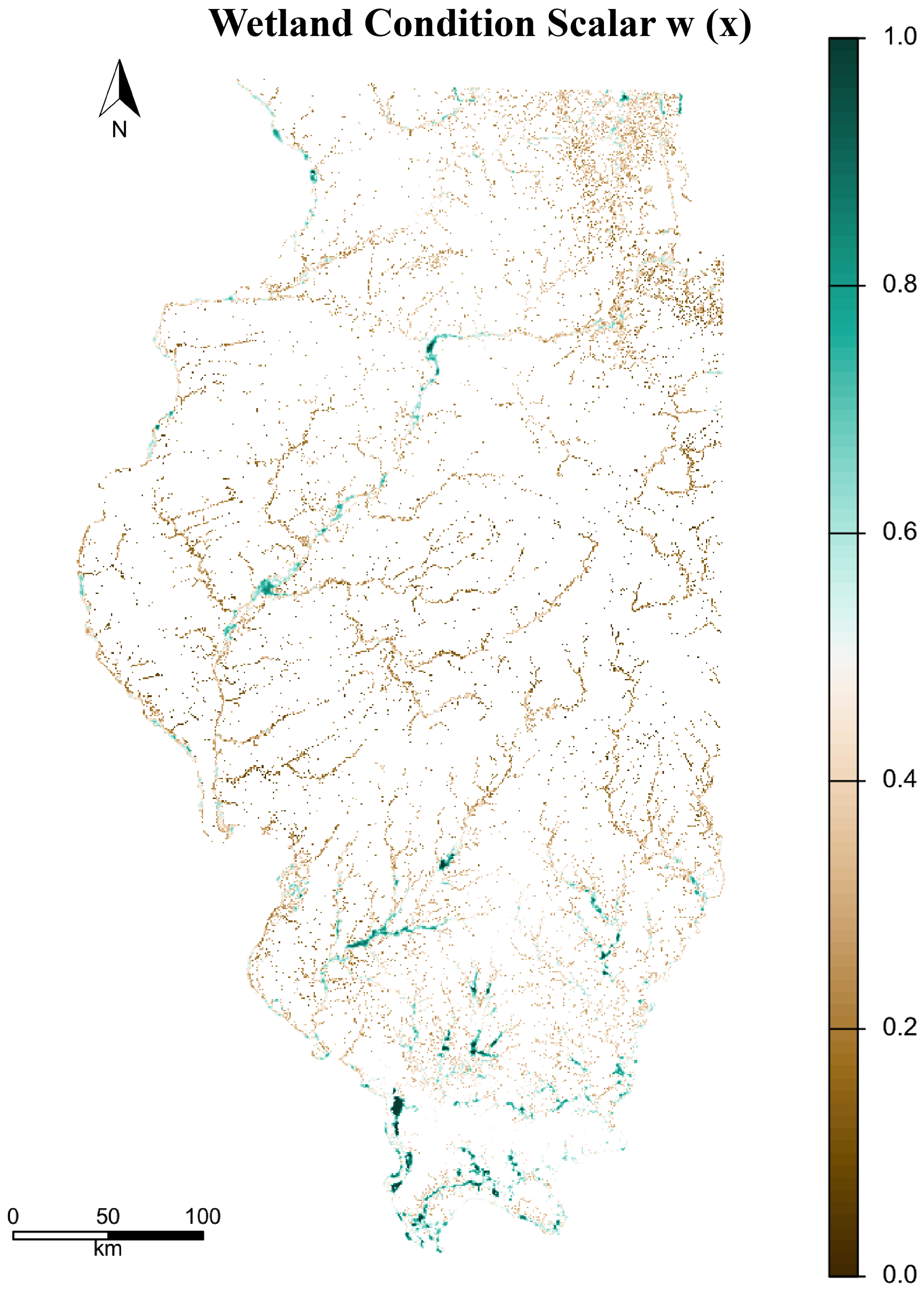
The final GAM produced a statewide 30-m surface of predicted floristic condition for Illinois vegetated palustrine wetlands (Figure 2). The model included a two-dimensional geographic smooth, landscape disturbance within 250 m, vegetated-wetland density within 1 km, and levee context. Seeded 50-km, five-fold spatial-block cross-validation yielded a pooled CV $R^2$ of 0.261, a mean-fold CV $R^2$ of 0.251, an RMSE of 0.727, and an MAE of 0.572 across the 244 CTAP sites. Basis-dimension checks indicated adequate smooth specification, and residual spatial autocorrelation was not significant (Moran’s $I=0.020$, permutation $p=0.202$).

Predicted $Q\left(x\right)$ values ranged from 1.586 to 4.935 and were transformed to the condition scalar $w\left(x\right)$ using the empirical two-anchor reference-condition transformation in Equation (2). The statewide mean condition scalar was 0.502. Approximately 0.1% of mapped wetland cells were clamped to $w\left(x\right)=0$, and 1.5% were clamped to $w\left(x\right)=1$. Summing condition-weighted area across the state produced a habitat-condition account of 198,280 condition-weighted hectares.

The mapped surface showed broad regional variation in predicted floristic condition. Higher values occurred in parts of southern Illinois and in selected wetland complexes elsewhere in the state, while lower values were widespread across intensively modified agricultural landscapes. These patterns should be interpreted as statewide screening results rather than site-level predictions. The geographic smooth contributed to the model, but the smooth-only model had low predictive performance, indicating that the condition surface was not reducible to a simple north–south trend.

Across alternative empirical reference-anchor definitions, the statewide mean condition scalar ranged from 0.432 to 0.604 around the central value of 0.502. Because these alternatives were monotone transformations of the same predicted condition surface, spatial rankings were invariant: Spearman correlations were 1.000 and top-decile overlap was complete across all tested definitions. This analysis demonstrates sensitivity of the account magnitude to anchor choice, not independent validation of the underlying condition model.

The spatial distribution of CTAP monitoring sites, distance to the nearest training site, and prediction standard error are shown in Figure S1 to document training-data coverage, spatial support, and prediction uncertainty.

4.2. Statewide Physical and Monetary Accounts

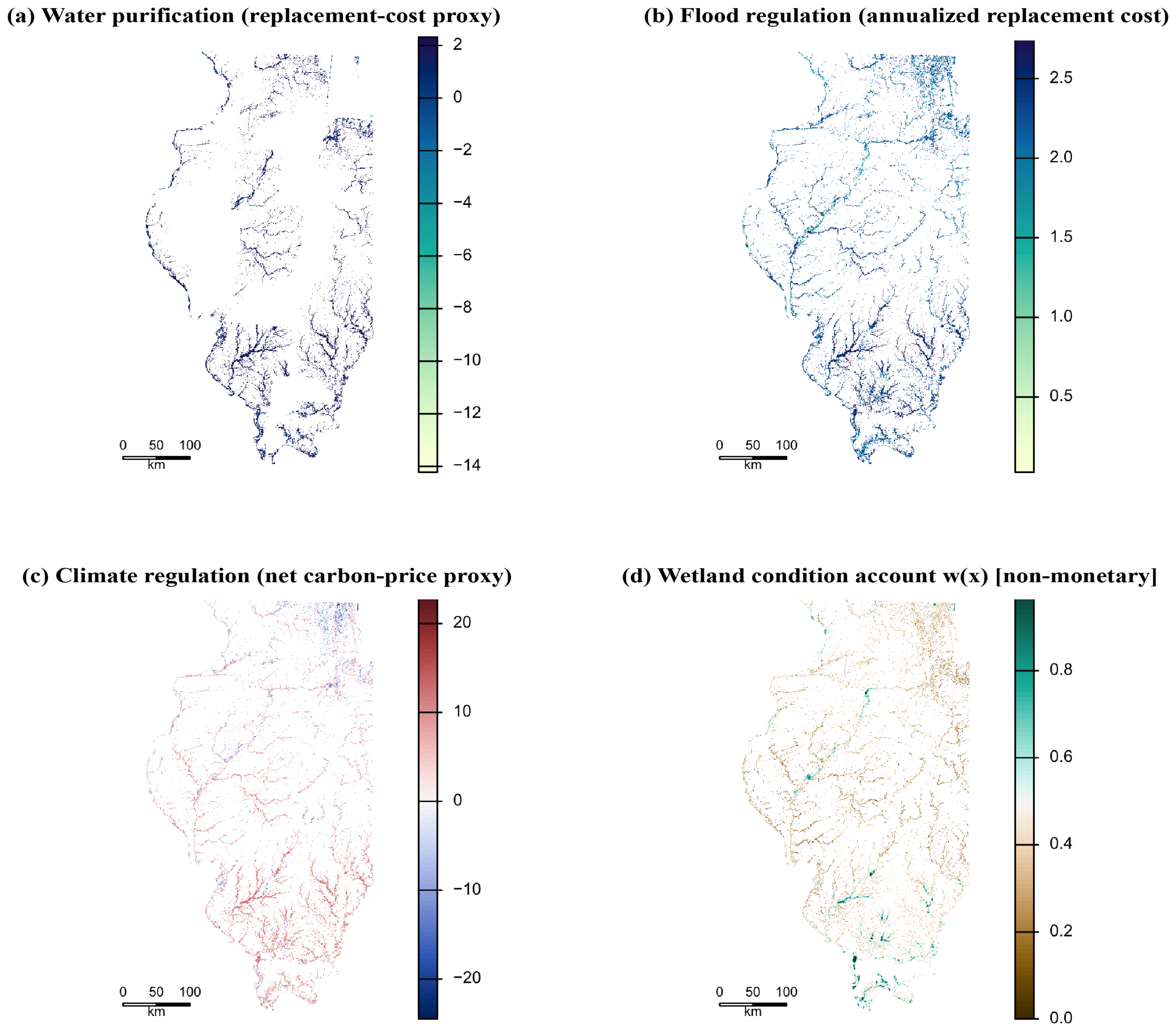
Under the central scenarios, Illinois vegetated wetlands produced a combined monetary proxy subtotal of approximately USD 1408.6 million yr⁻¹. This subtotal comprised USD 1048.5 million yr⁻¹ from the annualized surface-storage replacement-cost scenario for flood regulation, USD 338.0 million yr⁻¹ from the nitrogen-removal replacement-cost scenario, and USD 22.1 million yr⁻¹ from the carbon-price translation of net greenhouse-gas flux. The nonmonetary habitat-condition account was reported separately as 198,280 condition-weighted hectares and was not included in the monetary subtotal.

Flood regulation represented approximately 74% of the central monetary proxy subtotal, water purification 24%, and climate regulation 2%. These percentages describe the relative magnitude of three different translation scenarios and should not be interpreted as shares of observed social benefit. The flood estimate is particularly sensitive to the selected design storm and infrastructure-cost assumptions and represents the annualized cost of constructing equivalent detention capacity rather than realized avoided flood damage.

Across the full vegetated-wetland extent of approximately 976,800 acres, the central monetary proxy subtotal corresponds to about USD 1442 acre⁻¹ yr⁻¹. The account-specific averages are approximately USD 1073 acre⁻¹ yr⁻¹ for flood regulation, USD 346 acre⁻¹ yr⁻¹ for water purification, and USD 23 acre⁻¹ yr⁻¹ for climate regulation. These statewide averages are arithmetic summaries across the full mapped extent and do not represent parcel-level values (Figure 3).

For broad contextual comparison only, the central monetary proxy subtotal was placed alongside reported Illinois cropland cash rents. The 2025 statewide average cash rent was USD 264 per acre, with projected rents varying by land quality [64,65]. Cash rent is a realized private return to land, whereas the wetland figures are transferred carbon-price and replacement-cost proxies for public regulating services. The measures are not directly equivalent, the wetland and cropland parcels were not spatially matched, and conversion, drainage, production, transaction, and opportunity costs were not included.

The underlying physical accounts also differed substantially. Under the central water-purification scenario, routed and load-gated nitrogen removal totaled 57.7 million kg N yr⁻¹. Climate regulation was calculated from net greenhouse-gas flux using the IPCC AR6 biogenic methane GWP₁₀₀ of 27.0. Flood regulation was expressed physically as modeled detention volume under the 10-year design-storm scenario and monetarily as its annualized surface-storage replacement cost. Flood calculations were available only where the required hydrologic soil-group and land-cover inputs were present; cells without sufficient physical input data were not assigned a flood value (

Table 6. Combined monetary proxy subtotal by wetland category under the central scenarios.

Wetland Category	Count (Cells)	Monetary Proxy Subtotal	Share of Subtotal
		($M yr−1)	(%)
Bottomland Forest	2,919,523	1117.7	79.3
Shallow Marsh/Wet Meadow	554,541	109.0	7.7
Shrub-Scrub Wetlands	187,595	49.5	3.5
NLCD 90 Remainder (Woody)	483,621	85.8	6.1
NLCD 95 Remainder (Emergent)	246,800	46.7	3.3
Total	4,392,080	1408.6	100.0

Notes. The subtotal combines the central climate-regulation carbon-price proxy, water-purification replacement-cost proxy, and annualized flood-regulation surface-storage replacement-cost proxy. The statewide components are USD 22.1 million yr⁻¹ for climate regulation, USD 338.0 million yr⁻¹ for water purification, and USD 1048.5 million yr⁻¹ for flood regulation. The category values may not sum exactly to the displayed statewide total because of rounding. Habitat condition is reported separately in condition-weighted hectares and is not included in the monetary subtotal. The monetary estimates are scenario-based proxies rather than realized revenue, observed avoided costs, or net social benefits. The condition scalar $w\left(x\right)$ is not applied to any of the three monetary accounts.

).

4.3. Differences Among Wetland Categories

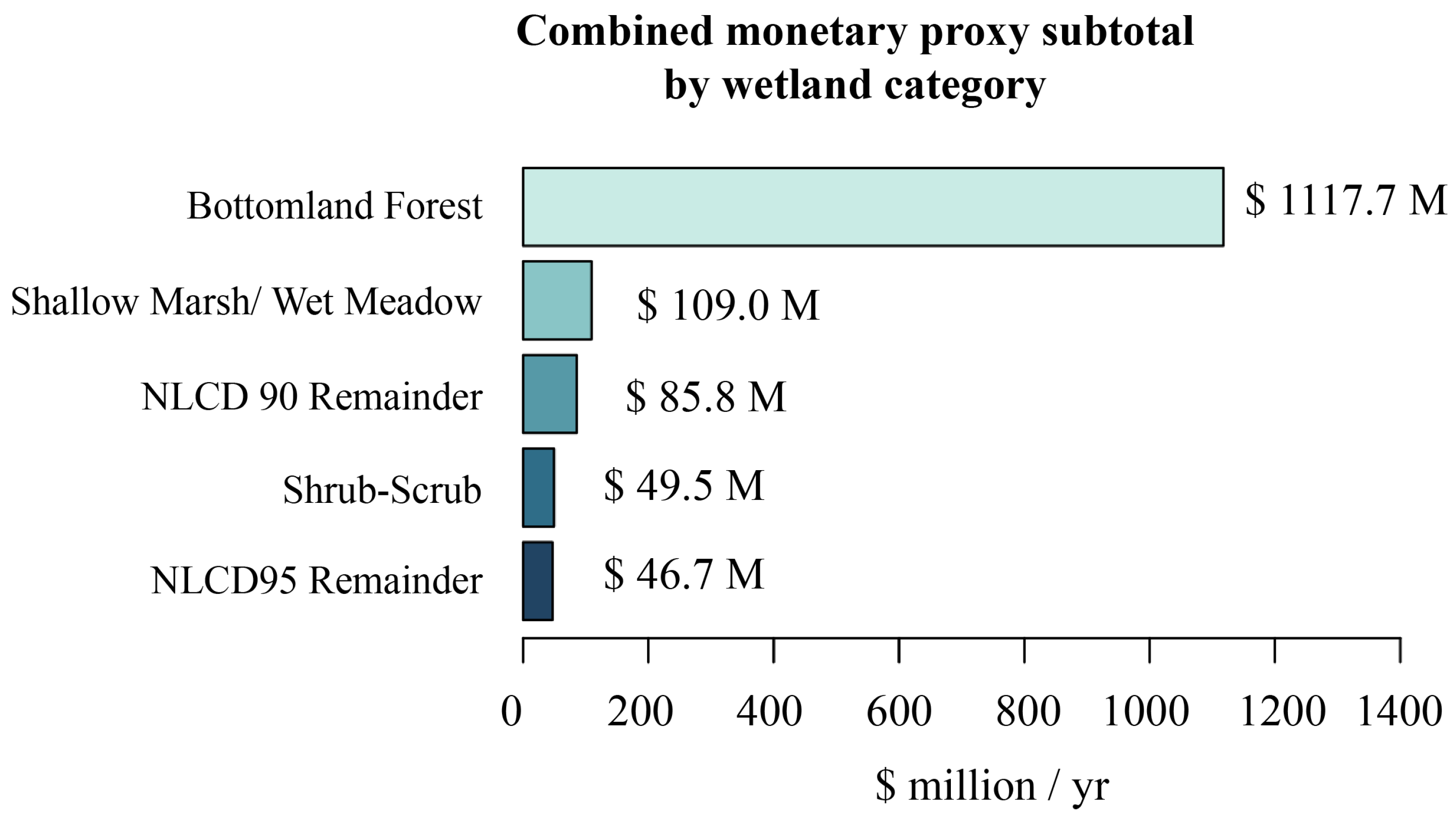
The combined monetary proxy subtotal varied substantially across the five vegetated-wetland categories (Figure 4). Bottomland Forest accounted for the largest total, approximately $1117.7 million yr⁻¹, or 79.3% of the statewide monetary proxy subtotal. This category also represented 2,919,523 cells, equivalent to approximately 66.5% of the mapped vegetated-wetland extent. Its share of the monetary subtotal therefore exceeded its share of wetland area, primarily because much of the modeled flood storage and routed nitrogen-removal capacity occurred in this category.

Shallow Marsh and Wet Meadow contributed approximately USD 109.0 million yr⁻¹, followed by the NLCD 90 Remainder at USD 85.8 million yr⁻¹, Shrub-Scrub Wetlands at USD 49.5 million yr⁻¹, and the NLCD 95 Remainder at USD 46.7 million yr⁻¹. These category totals combine the central climate-regulation carbon-price proxy, water-purification replacement cost proxy, and annualized flood-regulation surface-storage replacement-cost proxy. They should not be interpreted as observed benefits or realized revenues.

Differences among categories reflected both their mapped extent and the service-specific physical inputs used in each account. Flood regulation varied with land cover, hydrologic soil group, water regime, and the specified counterfactual. Water purification varied with wetland position in the routed nitrogen network and the load delivered to each reach. Climate regulation varied with category-specific carbon-sequestration and methane assumptions. Habitat condition was evaluated separately in condition-weighted hectares and was not included in the monetary category totals.

4.4. Protection-Gap Screening

The protection classification of Peterson et al. [11] was used as an external overlay rather than as a modeled component of the wetland accounts. The canonical vegetated-wetland raster and habitat-condition surface were intersected with the four protection tiers to identify where mapped wetland extent and modeled ecological condition coincide with different levels of institutional protection. The classification covered approximately 3174 km² of the 3953 km² statewide vegetated-wetland extent, equivalent to 80.3%. The remaining approximately 779 km² fell outside the four-tier classification and were retained as an unclassified category (

Table 7. Protection-gap screening by Peterson et al. (2025) [11] protection tier.

Protection Tier	Wetland Area	Share of Classified Area	Condition-Weighted Area	Share of Statewide Habitat Account	Share of Classified Habitat Account
	(km2)	(%)	(ha)	(%)	(%)
Tier 1: Biodiversity protection (GAP 1–2)	663.1	20.9	39,061	19.7	23.8
Tier 2: County ordinance	211.1	6.7	8531	4.3	5.2
Tier 3: Multiple uses (GAP 3)	76.0	2.4	6426	3.2	3.9
Tier 4: Unprotected	2223.8	70.1	109,885	55.4	67.0
Classified total	3174.0	100.0	163,903	82.7	100.0
Outside Peterson et al. classification	779.0	—	34,377	17.3	—
Statewide total	3953.0	—	198,280	100.0	—

Notes. Protection tiers were treated as an external screening overlay and were not used to construct the wetland accounts. Condition-weighted area equals mapped wetland area multiplied by the condition scalar $w\left(x\right)$. Percentages in the statewide-account column use 198,280 condition-weighted hectares as the denominator. Percentages in the classified-account column use 163,903 condition-weighted hectares within the Peterson et al. [11] classification. Cells outside the four-tier classification were retained in statewide totals but excluded from percentages calculated within the classified area. The table does not determine parcel-level legal status or conservation priority.

).

Within the classified wetland extent, approximately 2223.8 km², or 70.1%, occurred in Tier 4, the lowest-protection category. Because the monetary service accounts were substantially revised, the former protection-tier monetary totals were removed. The protection-gap results reported here therefore focus on classified wetland extent and the nonmonetary habitat-condition account.

The nonmonetary habitat-condition account totaled 198,280 condition-weighted hectares statewide. Of this total, 109,885 condition-weighted hectares occurred in Tier 4, representing 55.4% of the statewide habitat-condition account and 67.0% of the 163,903 condition-weighted hectares within the classified area. A further 34,377 condition-weighted hectares, or 17.3% of the statewide account, occurred outside the Peterson et al. [11] classification.

These results identify a spatial mismatch between modeled habitat condition and stronger institutional protection, but they do not establish parcel-level legal status or conservation priority. Protection-tier results are therefore interpreted as a screening layer to be considered together with ecological condition, service-specific physical outputs, feasibility, ownership, restoration potential, and other planning constraints.

5. Discussion and Conclusions

This study addresses a practical translation problem in wetland planning. Wetland evidence is often available, but it rarely arrives in a form that can directly support statewide spatial screening, comparison among wetland types, or early planning decisions. By linking ecosystem extent, ecological condition, physical service flows, and service-specific monetary proxies, the framework organizes heterogeneous evidence into spatially explicit and auditable accounts. Its contribution lies in the translation structure rather than in the creation of new ecological or valuation coefficients.

A central feature of the revised framework is the separation of ecological condition from monetary service translation. Floristic condition is reported through a nonmonetary habitat-condition account measured in condition-weighted hectares, while climate regulation, water purification, and flood regulation are estimated using service-specific physical models. The condition scalar $w\left(x\right)$ is not used to adjust any of the three monetary accounts. This separation avoids treating floristic integrity as a causal multiplier of ecosystem-service performance and preserves the distinction between ecological condition and monetary proxy values.

The habitat-condition account nevertheless adds planning-relevant information that would be absent from a uniform per-area treatment of wetland extent. It distinguishes areas of relatively higher and lower predicted floristic condition across the statewide wetland mask and can therefore support screening for closer ecological assessment, restoration feasibility analysis, or potential conservation attention. Because the GAM has modest spatial cross-validation performance, these outputs should be interpreted as regional screening surfaces rather than site-level condition estimates or regulatory thresholds.

Under the central scenarios, flood regulation contributed the largest share of the combined monetary proxy subtotal, followed by water purification and climate regulation. This ordering reflects the assumptions and units of three different translation methods rather than a common measure of realized social benefit. The flood account represents the annualized replacement cost of modeled surface-storage capacity, the water account represents the replacement cost of routed and load-gated nitrogen removal, and the climate account applies transferred policy-price scenarios to net greenhouse-gas flux. The subtotal should therefore be interpreted as a screening comparison among monetary proxies, not as an estimate of total economic value.

The climate account also demonstrates why wetland categories should not be treated as uniformly positive carbon assets. Methane emissions offset or exceed carbon sequestration in some emergent wetland categories under the central assumptions, whereas woody wetland categories generally retain positive net climate-regulation values. These category-specific tradeoffs support the use of multiple accounts rather than a single aggregate indicator when comparing wetland types or evaluating planning alternatives.

Bottomland Forest accounted for the largest share of the combined monetary proxy subtotal. This pattern reflects both its dominant share of mapped vegetated-wetland extent and the service-specific physical inputs associated with the category. Other categories contributed smaller statewide totals but displayed different combinations of climate, nitrogen-removal, flood-storage, and habitat-condition outcomes. Planning interpretations should therefore consider both total contribution and service composition rather than treating the statewide subtotal as a complete ranking of wetland types.

The protection-gap overlay provides a policy-context screening layer rather than a direct measure of legal vulnerability or conservation priority. Tier 4 contained 70.1% of the classified vegetated-wetland area and 67.0% of the condition-weighted habitat area within the classified domain. A further 779 km² of vegetated wetland occurred outside the four-tier classification. These results identify where ecological condition coincides with weaker or unclassified institutional protection, but parcel-level decisions would still require information on ownership, jurisdiction, restoration feasibility, hydrologic connectivity, development pressure, and local planning objectives.

The framework builds on earlier work calling for ecological characteristics to be incorporated more explicitly into ecosystem-service assessment, but it does so by maintaining separate condition and service accounts rather than by multiplying transferred values by a single condition factor. The Peterson et al. [11] classification is used only as an external overlay, and the contribution is the integration of independently constructed extent, condition, physical-service, monetary-proxy, and protection-context layers. The climate account also extends the Illinois wetland carbon analysis of Pang and Deal [39] by translating net greenhouse-gas flux after accounting for methane emissions.

The comparison with Illinois cropland cash rent is retained only as a broad contextual benchmark. Cash rent is a realized private return to land, whereas the wetland estimates are carbon-price and replacement-cost proxies for public regulating services. They are not directly equivalent, the parcels were not spatially matched, and the analysis does not include drainage, conversion, production, transaction, or opportunity costs. The comparison therefore illustrates the difference between private land returns and public-service proxies but does not demonstrate that wetland service value exceeds the value of agricultural conversion.

The framework also illustrates the value and limits of a floristic condition account. Four-layer Mean C provides an ecologically interpretable basis for mapping vegetation-based wetland condition because coefficients of conservatism distinguish disturbance-tolerant species from species associated with less-disturbed ecological settings. However, the resulting condition scalar $w\left(x\right)$ is not a calibrated multiplier for nitrogen removal, flood detention, carbon regulation, or any other individual ecosystem service. Floristic quality is therefore used only as a spatially continuous indicator for the nonmonetary habitat-condition account and not as a complete measure of biodiversity or ecological function.

Several methodological limitations follow from the statewide screening design. First, the final condition model has modest predictive skill. Seeded 50-km spatial-block cross-validation produced a pooled CV $R^2$ of 0.261, a mean-fold CV $R^2$ of 0.251, an RMSE of 0.727, and an MAE of 0.572. Although residual spatial autocorrelation was not significant, these diagnostics do not support site-level prediction or regulatory classification. The condition surface is best interpreted as a regional screening layer that introduces empirically modeled spatial variation while retaining the need for field-based assessment.

The absolute magnitude of the habitat-condition account also depends on the empirical anchor definition. Across the tested reference-condition scenarios, the statewide mean $w\left(x\right)$ ranged from 0.432 to 0.604 around the central value of 0.502. Spatial rankings were unchanged because the alternatives were monotone transformations of the same predicted condition surface: Spearman correlations were 1.000 and top-decile overlap was complete. This result demonstrates robustness of spatial ordering to the anchor choice, but it does not constitute independent validation of the underlying condition model.

A second limitation concerns temporal alignment. The floristic response was calculated as a site-level mean across CTAP observations collected from 1997 to 2022, whereas landscape disturbance and wetland-density predictors were derived from contemporary spatial datasets. The model therefore does not reconstruct changes in surrounding land cover over the monitoring period. Associations between floristic condition and landscape predictors should be interpreted as screening-level spatial relationships rather than time-matched causal effects.

A third limitation concerns the service accounts, which combine transferred physical parameters, spatial models, and monetary proxies drawn from different sources and scales. The water-purification account does not model in-stream attenuation and therefore represents an upper-delivery screening scenario. The flood account represents modeled runoff detention and the annualized cost of constructing equivalent surface-storage capacity; it does not estimate downstream stage reduction, avoided property damage, human-safety benefits, or the full range of floodplain processes. The climate account depends on category-level sequestration and methane assumptions and transferred carbon-price scenarios. These monetary outputs should therefore be interpreted as scenario-based proxies rather than realized expenditure, revenue, or net social benefit.

The framework does not provide a monetary biodiversity account. Habitat condition is reported in condition-weighted hectares and remains separate from the climate-regulation, water-purification, and flood-regulation monetary subtotal. This separation avoids combining incompatible value concepts and applying a single transferred biodiversity value uniformly across the state.

By preserving separate information on wetland extent, habitat condition, physical service flows, monetary proxies, and protection context, the framework provides a transparent basis for linking ecological evidence to land-use decisions. In this way, it contributes to sustainable development by supporting the monitoring, prioritization, and adaptive management of wetland resources within broader regional sustainability strategies.

Future refinement should proceed in three directions. First, independent field data could be used to validate the condition surface and to test relationships between floristic integrity and service-specific outcomes such as nitrogen retention, hydrologic storage, habitat structure, and faunal indicators. Such analyses should develop service-specific functional relationships rather than assume that one condition scalar applies uniformly across services. Second, uncertainty analysis could propagate model, parameter, routing, counterfactual, and monetary-transfer uncertainty rather than relying primarily on account-specific scenarios and one-way sensitivity tests. Third, the framework could be extended beyond vegetated palustrine wetlands to a broader statewide wetland and open-water typology, while preserving separate modeling rules for ecological condition and each physical service.

In applied planning, the accounting structure can be linked to retention, restoration, and land-use scenarios to compare how wetland extent, habitat condition, and physical service flows change under alternative decisions. Alignment on a common 30-m grid makes heterogeneous evidence easier to inspect, compare, and incorporate into statewide screening and early planning workflows. The framework does not remove uncertainty, establish parcel-level priorities, or replace site assessment, but it provides a consistent and auditable path from ecological evidence to planning-support information.