Sustainable Autoclaved Aerated Concrete Production Strategies Using a Hybrid Discrete-Event Simulation and Machine-Learning Surrogate Framework

Abstract

Autoclaved Aerated Concrete (AAC) is a lightweight construction material with strong relevance for energy-efficient and modular building systems, but its production remains constrained by steam-curing energy demand and carbon-intensive binders. This challenge is increasingly important as the AAC sector targets net-zero pathways and as cement and lime remain major contributors to life-cycle emissions in AAC products. This study develops an optimization framework for sustainable AAC production that leverages machine-learning surrogates for discrete-event simulations. We first construct a discrete-event factory model that represents mix preparation, mould pouring and rising, cutting, autoclaving, unloading, and product handling. We then couple the simulation to a ${\mathrm{CO}}_2$e and cost model and generate 116,640 production scenarios. Machine-learning surrogate models are trained to predict total ${\mathrm{CO}}_2$e emissions, cost, and production time, and a gradient-based optimization procedure is used to identify operating strategies under different carbon, cost, time, and balanced priorities. The results show that, autoclaving time, electricity carbon intensity, and cement use are the two most important environmental levers. The carbon–cost and carbon-priority strategies produced the lowest predicted emissions, approximately 1292 kg CO₂e, and selected the lowest electricity emission factor and cement mass considered in the design space, 0.05 kg CO₂e/kWh and 400 kg, respectively. The time-priority strategy produced the shortest predicted production time but the highest predicted emissions and cost, demonstrating a clear carbon–cost–time trade-off under the model assumptions. The proposed framework provides a practical decision-support tool for AAC manufacturers to compare production strategies, quantify trade-offs, and identify lower-carbon operating regimes before implementation.

1. Introduction

Sustainable construction is now central to reducing the climate impact of the built environment, which accounts for a large share of global energy demand and energy- and process-related ${\mathrm{CO}}_2$ emissions [1]. This creates strong pressure to develop construction materials that reduce embodied carbon while preserving performance, durability, affordability, and scalability. Autoclaved Aerated Concrete (AAC) is a lightweight mineral material with low density, dimensional stability, fire resistance, and strong thermal insulation, making it attractive for sustainable and modular building applications [2]. AAC is produced by mixing siliceous material, cement, lime, gypsum, water, and aluminum powder into a slurry, which expands through gas generation, forms a porous green cake, and is then pre-cured, cut, separated, and hardened in autoclaves under saturated steam at elevated temperature and pressure [3]. This steam-curing stage is essential for strength development and dimensional stability, but it is also one of the most energy-intensive factory operations. Therefore, AAC decarbonization requires attention to both upstream binder-related emissions, especially cement and lime, and operational emissions from steam generation and autoclaving [2,4]. Optimizing autoclave operation, electricity sourcing, heat demand, and binder use is consequently a practical pathway for reducing the carbon footprint of AAC production.

Life-cycle assessment (LCA) has been widely used to quantify the environmental performance of construction materials and to identify the production stages that dominate embodied impacts. For Autoclaved Aerated Concrete (AAC), existing LCA studies consistently show that environmental performance depends on both material inputs and factory operations. Ramagiri et al. [5] developed a cradle-to-gate LCA for autoclaved aerated fly ash and concrete block production in China using ${\mathrm{1 m}}^3$ of product as the functional unit. Their study identified fly ash slurry production, lime grinding, and steam curing as key process contributors. It also showed that cement, lime, and natural gas were the dominant material and energy contributors to overall environmental impact. These findings are important because they connect AAC emissions to both binder production and autoclave-related thermal demand.

Other studies extend AAC assessment beyond factory-gate production. Reyes-Quijije et al. [6] evaluated aerated concrete blocks in a building case study in Guayaquil, Ecuador, and compared them with conventional masonry materials. Their analysis linked material choice to structural weight reduction and environmental performance at the building scale. Fouad et al. [7] examined the environmental performance of AAC in the United States and emphasized its potential as a lower-impact wall material when assessed against conventional alternatives. At the sector level, the European Autoclaved Aerated Concrete Association reported that most cradle-to-grave AAC emissions arise from cement and lime production, while AAC manufacturing itself contributes a smaller but still operationally relevant share [2]. This distinction is central for decarbonization because raw-material substitution and factory energy optimization target different parts of the life cycle.

Recent LCA work has also addressed circularity and alternative raw materials. Volk et al. [8] assessed post-demolition AAC recycling options and found that closed-loop recycling into new AAC production can improve environmental performance compared with landfilling. This supports circular-economy strategies for reducing primary raw-material demand. Emerging studies further investigate alternative silica or ash sources, including municipal solid-waste incineration fly ash, high-volume fly ash, and tailings sand, while combining mechanical performance with environmental assessment [9,10]. These studies show that AAC decarbonization cannot be reduced to a single intervention. It requires coordinated changes in binders, energy supply, autoclave operation, recycling pathways, and production planning.

Overall, the LCA literature provides a clear foundation for AAC sustainability assessment. It identifies cement and lime as major embodied-emission drivers and steam curing as a key factory-stage energy demand. However, most existing studies evaluate fixed production scenarios or compare material alternatives. Fewer studies connect LCA-style emission accounting with dynamic factory simulation, machine-learning surrogates, and optimization. The present work addresses this gap by coupling a discrete-event AAC production model with ${\mathrm{CO}}_2$e and cost calculations, generating a large simulation dataset, and using surrogate-guided optimization to evaluate carbon-, cost-, time-, and balanced operating strategies.

Discrete-event simulation methods provide a rigorous framework for representing complex construction-material production systems. They capture individual production entities, finite-capacity resources, queues, transport operations, and local interactions that generate system-level behaviour. This is important for AAC manufacturing because production performance depends on coordinated movement through mixing, mould filling, rising, cutting, autoclaving, unloading, and storage. Discrete-event simulation has been widely used in construction to study decentralized interactions, dynamic operations, productivity, logistics, and resource allocation [11,12]. Multi-agent and agent-based manufacturing models are also increasingly used to represent smart production systems because they can capture distributed decisions, autonomous resources, and adaptive coordination [13]. In the AAC context, this modelling strategy allows the factory to be evaluated as an integrated production system rather than as isolated process steps.

Artificial intelligence extends this simulation capacity by learning fast predictive models from simulated or observed production data. Machine-learning models can approximate the relationship between production settings, material use, energy demand, ${\mathrm{CO}}_2$e emissions, cost, and completion time. These surrogate models reduce the computational cost of scenario analysis and make optimization feasible over large design spaces. Indeed, the optimization of discrete and non-differentiable systems represents a fundamental challenge in operations research and machine learning. Classical gradient-based methods, such as stochastic gradient descent, cannot be directly applied to problems involving discrete variables or discontinuous decision functions. The straight-through estimator (STE), introduced by Bengio et al. [14], provides an elegant solution to this issue: during backpropagation, the derivative of the non-differentiable function is replaced with a smooth approximation (typically the identity function or a soft sigmoid), while maintaining discrete values during the forward pass.

Recent reviews show that AI is increasingly used in construction materials to support mixture design, property prediction, process optimization, durability assessment, sustainability analysis, and quality control [15]. We illustrate this in this work, with discrete-event simulations that preserve the operational and sequential dynamics of AAC production, while machine learning accelerates prediction and optimization. The resulting hybrid framework supports practical decision making by identifying lower-carbon, cost-aware, and time-efficient operating strategies before implementation in the physical factory.

More broadly, digital technologies are reshaping manufacturing by converting production lines into measurable, adaptive, and decision-oriented systems [16]. In construction-material manufacturing, this shift is especially important because production quality, energy demand, and carbon intensity depend on tightly coupled process variables, including material dosing, curing conditions, equipment utilization, and production scheduling [17]. Industry 4.0 tools, including sensors, data platforms, simulation, digital twins, and automated control, make it possible to track these variables across the production line and evaluate operational changes before implementing them in the factory [18,19]. For AAC production, such tools can support the systematic assessment of autoclave operation, steam demand, electricity sourcing, binder use, throughput, and cost. They therefore provide a practical pathway for linking productivity targets with decarbonization objectives.

In this work, we develop an integrated simulation and machine-learning framework for AAC production. We consider a discrete-event factory model, couple it to carbon-emission and cost calculations, and use the generated simulation data to train surrogate models that rapidly predict ${\mathrm{CO}}_2$e emissions, production cost, and completion time. The trained surrogate is then used to identify operating strategies under carbon-focused, cost-focused, time-focused, and balanced objectives. Using this framework, we identify the strategies that minimize carbon emissions, while also reducing the cost and time required for batch production. This framework provides a practical decision-support tool for AAC manufacturers. It allows production strategies to be tested computationally, trade-offs to be quantified before implementation, and lower-carbon operating regimes to be identified without disrupting factory operations.

2. Materials and Methods

2.1. Problem Description: Autoclaved Aerated Concrete Production Process

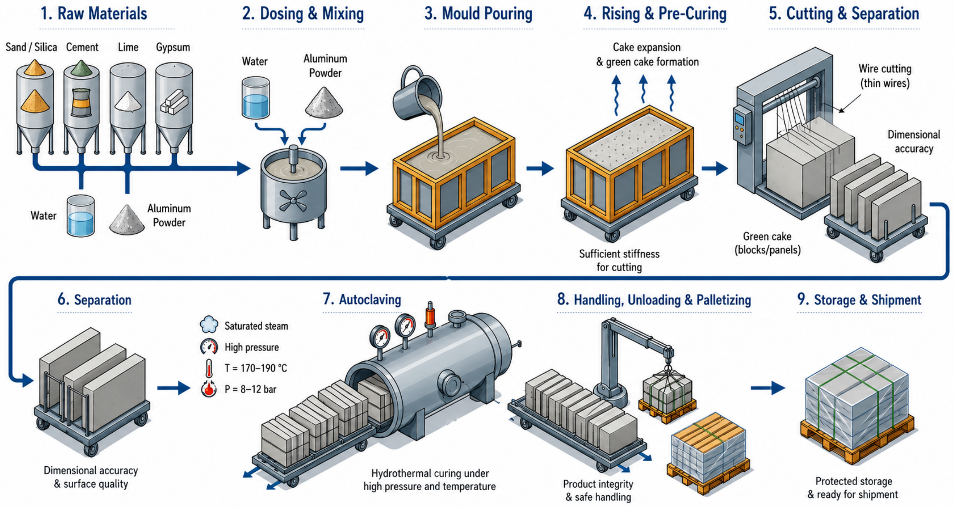
Autoclaved Aerated Concrete (AAC) is a lightweight precast construction material produced in a controlled industrial environment. Its cellular structure results from the reaction of aluminum powder within an alkaline cementitious slurry, which generates gas bubbles and expands the fresh mixture. The expanded material is then pre-cured, cut to the required dimensions, and hardened under saturated steam in autoclaves. This sequence gives AAC its characteristic low density, dimensional accuracy, and mechanical stability.

The AAC factory is a sequential manufacturing system. Material flows from raw-material preparation to mixing, casting, rising, cutting, separation, autoclaving, unloading, and palletizing. These stages are standard in industrial AAC production and are also the main stages represented in the considered AnyLogic AAC factory model [20,21]. The model follows production from raw materials to pallets of concrete blocks and supports analysis of factory capacity, waiting times, and resource utilization.

The production system includes the following main components:

• Raw-material preparation: Sand or other siliceous materials, cement, lime, gypsum, water, and aluminum powder are stored, prepared, and dosed. Accurate dosing controls slurry composition, aeration, density, and product quality.
• Mixing and mould pouring: The ingredients are mixed into a homogeneous slurry and poured into moulds. Aluminum powder initiates gas generation, which expands the mixture and forms the porous internal structure of AAC.
• Rising and pre-curing: Filled moulds are transferred to a rising area. The cake expands and gains sufficient stiffness for demoulding and cutting. This stage controls the transition from fluid slurry to stable green cake.
• Cutting and separation: The green cake is demoulded and cut into blocks or panels. The cut elements are then separated and prepared for autoclave loading. This stage determines dimensional accuracy and strongly affects downstream flow.
• Autoclaving: Cut elements are loaded into autoclaves and cured under saturated steam. Autoclaving promotes the formation of calcium-silicate-hydrate phases, including tobermorite, which contribute to strength, rigidity, and durability [22].
• Handling, unloading, and palletizing: Moulds, cakes, hardening cars, cranes, trolleys, and pallets move material between stations. After curing, products are unloaded, stacked, palletized, and transferred to storage or shipment.

The process begins with raw-material preparation and slurry mixing. The slurry is poured into moulds, where aeration produces volume expansion. After rising and pre-curing, the green cake is demoulded, cut, separated, and loaded onto hardening cars. The elements are then autoclaved, unloaded, palletized, and stored as finished AAC products.

From a modelling perspective, the AAC factory can be represented as a discrete-event production system. Each mould, cake, hardening car, or pallet is treated as an entity moving through a network of processing stations. Each station has finite capacity, processing time, queueing behaviour, and resource requirements. The model therefore captures both the physical sequence of production and the operational constraints that govern factory performance.

The main objective of the simulation is to evaluate and improve production performance. Relevant outputs include throughput, cycle time, queue length, waiting time, station utilization, autoclave occupancy, idle time, and the number of finished pallets produced over a planning horizon. These indicators make it possible to identify bottlenecks, test alternative resource allocations, assess transport and handling constraints, and quantify the effect of changes in processing times or factory layout. Figure 1 illustrates the simplified AAC production flow considered in this study.

The AAC production line is highly interdependent. A capacity limitation at one station can propagate through the entire factory. Limited autoclave availability can create queues after cutting. Slow mould circulation can reduce casting productivity. Insufficient handling capacity can increase idle time at otherwise productive stations. Therefore, local improvements must be evaluated at the system level.

2.2. Simulation Design

The AAC production system was implemented as a discrete-event manufacturing simulation in AnyLogic. The model follows the logic of the publicly available AnyLogic Cloud AAC factory model, which represents concrete production from raw materials to finished products through mix preparation, mould pouring, rising, cutting, separation, autoclaving, and unloading [20]. This structure is consistent with manufacturing simulation practice, where process models support capacity analysis, bottleneck identification, resource allocation, and safe evaluation of operational changes before implementation.

The public AnyLogic AAC factory model was used as the operational backbone for representing the main production flow, including slurry preparation, mould pouring, rising, cutting, autoclaving, unloading, and product movement. The original template primarily supports production-flow visualization, capacity analysis, and operational assessment. In this study, we extended this template into a sustainability-oriented decision-support model by adding stage-level ${\mathrm{CO}}_2$e accounting, electricity and thermal-energy calculations, material-emission calculations, production-cost calculations, parameter-variation routines, structured data export, and downstream machine-learning and optimization modules.

These modifications were introduced to make the simulation suitable for carbon and cost evaluation. The added emission module links each production stage to electricity use, thermal-energy demand, and material-related ${\mathrm{CO}}_2$e emissions. The cost module links material, electricity, and heat consumption to production cost. The parameter-variation and data-export routines allow thousands of alternative production configurations to be evaluated systematically. These extensions convert the public production-flow template into a framework for comparing AAC operating strategies, quantifying carbon–cost–time trade-offs, and identifying lower-carbon production regimes before implementation in a physical plant.

The simulation is organized around the Main agent. This agent contains the production stages, material-handling resources, routing blocks, storage elements, state variables, and data-export functions. The model tracks the movement of AAC cakes, moulds, trolleys, cranes, platforms, and autoclave resources through the production line. It also records production time, resource use, energy consumption, ${\mathrm{CO}}_2$e emissions, and cost. The structure therefore links operational behaviour to sustainability metrics within a single simulation environment.

2.2.1. Production-Flow Components

Table 1. Production-flow components in the AAC simulation model.

Component	Role in the Simulation
slurryPreparation	Prepares the AAC slurry before casting. This block represents the upstream mixing operation that supplies slurry to the casting stage.
waitSlurry	Holds production flow until slurry is available. It synchronizes material availability with mould processing.
pourSlurry	Transfers prepared slurry into moulds. It initiates the formation of the AAC cake.
casting	Represents mould filling and initial casting. It defines the start of the cake production cycle.
mouldProcessing	Controls mould preparation and circulation. It supports repeated use of moulds across production cycles.
risingArea	Represents the rising and pre-curing stage. The cake expands and gains sufficient stiffness before demoulding and cutting.
backTiltTable	Supports the transition from moulded cake to downstream handling. It represents tilting or positioning before cutting.
cuttingLine1	Represents the cutting stage. The green cake is cut into blocks or panels before separation.
greenSeparation	Represents separation of freshly cut elements. It prepares the cut AAC products for autoclave loading.
separator	Executes or supports the separation operation. It contributes to downstream flow organization before curing.
autoclaving	Represents steam curing in autoclaves. This stage is central to production capacity and thermal-energy demand.
unloading	Represents removal of cured AAC products from the autoclave system.
movingOut	Moves finished products out of the production process toward storage or shipment.

summarizes the main production-flow components embedded in the Main agent. These components define the transformation of raw slurry into finished AAC products.

These production-flow components reproduce the main AAC manufacturing sequence. The slurry is prepared, poured into moulds, allowed to rise, cut in the green state, separated, cured in autoclaves, unloaded, and moved out of the system. The model abstracts the detailed chemistry of AAC formation. It focuses on process timing, resource constraints, queueing, and throughput.

2.2.2. Material-Handling and Transport Components

Table 2. Material-handling and transport components in the AAC simulation model.

Component	Role in the Simulation
moulds	Represents the pool of moulds used for casting and circulation. Mould availability directly affects production continuity.
cakes	Represents AAC cakes moving through rising, cutting, separation, and autoclaving. Cakes are the main production entities.
platforms	Represents platforms used to support movement and positioning of cakes or moulds.
trolleys	Represents transport resources used to move products or platforms between stations. Trolley availability affects internal logistics.
tiltCrane	Represents the crane resource used around tilting and transfer operations.
liftingCrane	Represents lifting operations for moving cakes, moulds, or cured products. Crane capacity affects queueing and station idle time.
toRisingArea	Routes cast moulds or cakes toward the rising area.
fromRisingArea	Routes pre-cured cakes from the rising area to downstream processing.
toTiltCrane	Routes entities toward the tilt-crane operation.
fromBackTiltTable	Routes entities from the back-tilt table to the next production stage.
toUnloadCrane	Routes cured products toward unloading operations.
fromAutoclave	Routes products exiting autoclaves.
toOut	Routes finished AAC products out of the modelled production system.

summarizes the handling and transport components. These elements move cakes, moulds, platforms, and cured products between production stations.

The handling structure captures the fact that AAC production is not only a sequence of processing steps. It is also a material-flow system. Mould circulation, crane availability, trolley movement, and routing delays can create congestion and reduce effective capacity. The simulation therefore evaluates both processing resources and internal logistics.

2.2.3. Control, Queueing, and Decision Components

Table 3. Control, queueing, and routing components in the AAC simulation model.

Component	Role in the Simulation
queue	Stores entities waiting for downstream capacity. Queue length is an indicator of congestion and bottleneck formation.
hold	Temporarily blocks entities until a condition is satisfied. It supports synchronization between operations.
hold1	Provides an additional holding point for conditional process flow.
hold2	Provides a third holding point for synchronization and capacity control.
selectOutput	Selects the downstream path for entities. It supports routing decisions and process branching.
fromBackTiltTable	Controls transfer after tilting and before downstream processing.
fromAutoclave	Controls transfer after autoclave completion.
fromRisingArea	Controls transfer after the rising stage.

summarizes the control and queueing components. These blocks regulate flow, waiting, and routing decisions.

These components provide the logic required for discrete-event control. They ensure that entities advance only when resources, capacity, and process conditions allow. This is essential for representing finite-capacity manufacturing systems.

2.2.4. Model Functions

The model includes four main functions for emission calculation, data recording, dataset generation, and export.

Table 4. Functions used for calculation and data generation.

Function	Role in the Simulation
calculateEmissions	Computes stage-level and total ${\mathrm{CO}}_2$e emissions from energy use, material use, and emission factors. It links the production simulation to the emission model.
DBWrite	Writes simulation outputs to an internal database. It supports structured storage of run-level and process-level results.
generateDataset	Triggers the dataset-generation routine at the end of each simulation run. It organizes the simulation outputs for downstream analysis.
saveResultsToCSV	Exports collected results to CSV. The exported dataset is used for statistical analysis, machine-learning surrogate modelling, and optimization.

summarizes their roles.

These functions convert the simulation from a process-animation model into a data-generating decision-support model. They allow each simulated configuration to be evaluated using operational, economic, and environmental outputs.

2.2.5. Model Parameters

The model uses four parameter groups: capacity parameters, process-time and speed parameters, energy and emission parameters, and cost and production-horizon parameters.

Table 5. Capacity and storage parameters in the AAC simulation model.

Parameter	Interpretation
storageSize	Finished-product or intermediate storage capacity. It controls buffering and congestion.
mouldQuantity	Number of moulds available for casting and circulation. It controls casting continuity.
autoclaveN	Number of autoclaves available for steam curing. It controls batch-curing capacity.
trolleyN	Number of trolleys available for internal transport. It controls material-handling capacity.
bogeyN	Number of bogeys available for carrying cakes or products. It supports transport and staging.
numProductionLines	Number of active production lines. It controls parallel production capacity.
sandStorageSize	Storage capacity for sand. It affects raw-material availability.
gypsumStorageSize	Storage capacity for gypsum. It affects raw-material availability.
slurryStorageSize	Storage capacity for prepared slurry. It links upstream mixing with casting demand.
sandArrivalQuantity	Quantity of sand delivered per replenishment event.
gypsumArrivalQuantity	Quantity of gypsum delivered per replenishment event.
sandCriticalVolume	Reorder or critical threshold for sand storage.
gypsumCriticalVolume	Reorder or critical threshold for gypsum storage.

summarizes the main capacity parameters.

Capacity parameters determine whether the line can maintain flow under different production scenarios. They directly affect queue length, idle time, utilization, and throughput. The model records variables that describe process time, energy use, emissions, cost, production output, and run identification.

Table 6. Time and production variables recorded during simulation.

Variable	Interpretation
mixTimeActual	Actual time spent in mixing.
riseTimeActual	Actual time spent in rising or pre-curing.
cutTimeActual	Actual time spent in cutting.
autoTimeActual	Actual time spent in autoclaving.
totalTime	Total modelled production time.
totalTimeActual	Total actual production time recorded from the simulation.
timeDays	Simulation time expressed in days.
dayOutput	Daily production output.
totalBatches	Total number of produced batches.
selectedAutoclave	Autoclave selected for a given entity or operation.
selectedAutoclaveNumber	Index of the selected autoclave.
toUnloadCraneCount	Count of entities routed toward the unloading crane.

summarizes the main time and production variables.

These variables link factory operation to sustainability outcomes. They allow the model to identify which stages dominate energy use and carbon footprint. The resulting simulation design provides a complete computational representation of AAC production. It combines process flow, resource constraints, material handling, energy accounting, emission accounting, cost accounting, and dataset generation. This structure enables systematic comparison of production scenarios and provides the basis for surrogate modelling and optimization.

2.3. CO₂e Emission Model for AAC Production

We developed a stage-based ${\mathrm{CO}}_2$e emission model for Autoclaved Aerated Concrete (AAC) production. The model links the discrete-event factory simulation to material use, electricity demand, thermal-energy demand, production output, and project-level carbon footprint. It estimates emissions for each simulated production scenario and supports direct comparison of alternative operating policies.

The system boundary covers factory production from raw-material preparation to finished AAC products. The modelled stages include mix preparation, mould pouring and rising, cutting and separation, autoclaving, handling, unloading, and palletizing. This boundary captures the main operations represented in the simulation and the main production-related emission sources: embodied raw-material emissions, electricity use, and thermal energy for steam curing.

AAC emissions arise from two principal sources [23]. The first source is upstream material production, especially cement and lime. These materials have high carbon intensity because their production requires substantial energy input and includes process emissions from calcination. The second source is factory operation, especially autoclaving, which requires saturated steam at elevated temperature and pressure. Previous AAC life-cycle evidence indicates that cement and lime account for most AAC life-cycle emissions, while manufacturing contributes a smaller but operationally important share [2]. Electricity emission factors may be specified using national or regional grid factors, including the IEA emission-factor database [24]. Thermal-energy factors may be defined from the fuel used to generate steam following stationary-combustion accounting methods [25].

All process times generated by the simulation are recorded in minutes and converted to hours for energy calculations. Electrical power is expressed in kW, thermal power in ${\mathrm{kW}}_{\mathrm{th}}$, electrical energy in kWh, thermal energy in ${\mathrm{kWh}}_{\mathrm{th}}$, and emissions in kg ${\mathrm{CO}}_2$e.

2.3.1. Stage 1: Mix Preparation

The mixing stage combines silica slurry, cement, lime, aluminum powder, and water using electrically powered mixers. Emissions arise from electricity consumption and embodied material emissions. The electrical energy consumed during mixing is

$$Q_{\mathrm{mix},\mathrm{el}}=P_{\mathrm{mix}}·{\displaystyle \frac{T_{\mathrm{mix}}}{60}}.$$

(1)

The corresponding electricity-related emissions are

$$E_{\mathrm{mix},\mathrm{el}}=E{F}_{\mathrm{el}}·Q_{\mathrm{mix},\mathrm{el}}.$$

(2)

Material-related emissions are computed from input masses and emission factors:

$$E_{\mathrm{mix},\mathrm{mat}}=W_{\mathrm{cement}}·E{F}_{\mathrm{cement}}+W_{\mathrm{lime}}·E{F}_{\mathrm{lime}}+W_{\mathrm{al}}·E{F}_{\mathrm{al}}.$$

(3)

The total emissions from mix preparation are

$$E_{\mathrm{mix}}=E_{\mathrm{mix},\mathrm{el}}+E_{\mathrm{mix},\mathrm{mat}}.$$

(4)

Electricity emission factors are obtained from the IEA database [24]. Cement emissions are based on Andrew [23]. Lime emissions follow IPCC methodology [25]. Aluminum emissions are derived from the ecoinvent database [26].

2.3.2. Stage 2: Mould Pouring and Rising

During mould pouring and rising, the AAC mixture undergoes aeration and controlled thermal conditioning. This stage requires electrical and thermal energy. Electrical energy consumption is

$$Q_{\mathrm{rise},\mathrm{el}}=P_{\mathrm{rise},\mathrm{el}}·{\displaystyle \frac{T_{\mathrm{rise}}}{60}}.$$

(5)

Thermal energy consumption is

$$Q_{\mathrm{rise},\mathrm{heat}}=P_{\mathrm{rise},\mathrm{heat}}·{\displaystyle \frac{T_{\mathrm{rise}}}{60}}.$$

(6)

The associated electricity-related emissions are

$$E_{\mathrm{rise},\mathrm{el}}=E{F}_{\mathrm{el}}·Q_{\mathrm{rise},\mathrm{el}}.$$

(7)

The associated thermal-energy emissions are

$$E_{\mathrm{rise},\mathrm{heat}}=E{F}_{\mathrm{heat}}·Q_{\mathrm{rise},\mathrm{heat}}.$$

(8)

The total emissions from rising are

$$E_{\mathrm{rise}}=E_{\mathrm{rise},\mathrm{el}}+E_{\mathrm{rise},\mathrm{heat}}.$$

(9)

Heat emission factors are based on IPCC guidelines [25].

2.3.3. Stage 3: Cutting

Once the AAC cake reaches sufficient stiffness, electrically powered cutting machines divide it into blocks or panels. The electrical energy consumed during cutting is

$$Q_{\mathrm{cut},\mathrm{el}}=P_{\mathrm{cut}}·{\displaystyle \frac{T_{\mathrm{cut}}}{60}}.$$

(10)

The corresponding emissions are

$$E_{\mathrm{cut}}=E{F}_{\mathrm{el}}·Q_{\mathrm{cut},\mathrm{el}}.$$

(11)

2.3.4. Stage 4: Autoclaving

Autoclaving is the most energy-intensive production stage. It uses high-pressure steam curing and auxiliary electrical equipment. Electrical energy consumption during autoclaving is

$$Q_{\mathrm{auto},\mathrm{el}}=P_{\mathrm{auto},\mathrm{el}}·{\displaystyle \frac{T_{\mathrm{auto}}}{60}}.$$

(12)

Thermal energy consumption during autoclaving is

$$Q_{\mathrm{auto},\mathrm{heat}}=P_{\mathrm{auto},\mathrm{heat}}·{\displaystyle \frac{T_{\mathrm{auto}}}{60}}.$$

(13)

The electricity-related emissions are

$$E_{\mathrm{auto},\mathrm{el}}=E{F}_{\mathrm{el}}·Q_{\mathrm{auto},\mathrm{el}}.$$

(14)

The thermal-energy emissions are

$$E_{\mathrm{auto},\mathrm{heat}}=E{F}_{\mathrm{heat}}·Q_{\mathrm{auto},\mathrm{heat}}.$$

(15)

The total emissions from autoclaving are

$$E_{\mathrm{auto}}=E_{\mathrm{auto},\mathrm{el}}+E_{\mathrm{auto},\mathrm{heat}}.$$

(16)

2.3.5. Total Production Emissions

The total production carbon footprint per AAC cake is obtained by summing emissions across the modelled production stages:

$$C{F}_{\mathrm{prod}}=E_{\mathrm{mix}}+E_{\mathrm{rise}}+E_{\mathrm{cut}}+E_{\mathrm{auto}}.$$

(17)

This quantity is the main emission output of the production model. It allows direct comparison of simulated scenarios and quantifies how production timing, energy demand, material use, and autoclave operation affect the carbon footprint of AAC manufacturing.

2.3.6. Cost Model

The production cost per AAC cake is decomposed into material, electricity, and thermal-energy costs. Material cost is

$$C_{\mathrm{mat}}=c_{\mathrm{cement}}{W}_{\mathrm{cement}}+c_{\mathrm{lime}}{W}_{\mathrm{lime}}+c_{\mathrm{al}}{W}_{\mathrm{al}}.$$

(18)

Electricity cost is

$$C_{\mathrm{el}}=c_{\mathrm{el}}\left(Q_{\mathrm{mix},\mathrm{el}}+Q_{\mathrm{rise},\mathrm{el}}+Q_{\mathrm{cut},\mathrm{el}}+Q_{\mathrm{auto},\mathrm{el}}\right).$$

(19)

Thermal-energy cost is

$$C_{\mathrm{heat}}=c_{\mathrm{heat}}\left(Q_{\mathrm{rise},\mathrm{heat}}+Q_{\mathrm{auto},\mathrm{heat}}\right).$$

(20)

The total production cost per AAC cake is

$$C_{\mathrm{total}}=C_{\mathrm{mat}}+C_{\mathrm{el}}+C_{\mathrm{heat}}.$$

(21)

In the baseline simulation, the cost terms are computed from material use, electricity demand, and thermal-energy demand, and therefore do not by themselves imply that higher total cost reduces autoclaving duration. For the post-processing trade-off analysis, we introduce the hypothesis that shorter autoclaving cycles require additional curing-related process intensification cost, representing higher steam intensity, auxiliary energy use, process control, or quality-assurance effort needed to maintain product quality under reduced curing time.

$$C_{\mathrm{acc}}=\eta \left(T_{\mathrm{auto},\max }-T_{\mathrm{auto}}\right),$$

(22)

$$C_{\mathrm{total}}^{*}=C_{\mathrm{total}}+C_{\mathrm{acc}},$$

(23)

where $C_{\mathrm{acc}}$ is the acceleration cost, $T_{\mathrm{auto},\max }$ is the longest autoclaving duration in the design space, $T_{\mathrm{auto}}$ is the selected autoclaving duration, and $\eta$ is the acceleration-cost coefficient.

2.3.7. Project-Level Scaling

Let $B_{\mathrm{day}}$ denote the number of batches produced per day and $D_{\mathrm{sim}}$ the number of simulated production days. The total number of batches produced over the study horizon is

$$N_{\mathrm{batches}}=B_{\mathrm{day}}·D_{\mathrm{sim}}.$$

(24)

The total project-level carbon footprint is

$$C{F}_{\mathrm{project}}=C{F}_{\mathrm{prod}}·N_{\mathrm{batches}}.$$

(25)

The total project-level production cost is

$$C_{\mathrm{project}}=C_{\mathrm{total}}·N_{\mathrm{batches}}.$$

(26)

These project-level quantities place all scenarios on a common planning horizon. They support sustainability-oriented optimization by linking production decisions to carbon footprint, cost, and operational performance. The added ${\mathrm{CO}}_2$e emission parameters are provided in

Table 7. Energy, emission, material, and cost parameters in the AAC simulation model.

Parameter	Interpretation
pMix	Electrical power demand of the mixing stage.
pRiseHeat	Thermal power demand during rising or pre-curing.
pRiseEl	Electrical power demand during rising or pre-curing.
pCut	Electrical power demand of the cutting stage.
pAutoHeat	Thermal power demand during autoclaving.
pAutoEl	Auxiliary electrical power demand during autoclaving.
efElectricity	Electricity emission factor.
efHeat	Thermal-energy emission factor.
efCement	Cement emission factor.
efLime	Lime emission factor.
efAluminum	Aluminum powder emission factor.
wCement	Cement mass per AAC cake or batch.
wLime	Lime mass per AAC cake or batch.
wAluminum	Aluminum powder mass per AAC cake or batch.
cElectricity	Unit cost of electricity.
cHeat	Unit cost of thermal energy.
cCement	Unit cost of cement.
cLime	Unit cost of lime.
cAluminum	Unit cost of aluminum powder.

. To facilitate result interpretation and reduce the computational time associated with data generation, we assume that all emission factors and process-associated costs are constant.

2.4. Data Generation

We generated the dataset through a large-scale parameter-variation experiment. The experiment used the discrete-event AAC factory model to evaluate how production capacity, resource allocation, process timing, electricity intensity, and cement use affect operational, economic, and environmental outcomes. We conducted 116,640 simulation runs. The parameter-variation experiment generated 116,640 simulation records through full factorial enumeration of all admissible parameter combinations, corresponding to $8\times 5\times 3\times 4\times 3\times 3\times 3\times 9$ candidate settings. The full simulation experiment was executed on an Apple M4 processor and completed in approximately 4.845 h. Training the four surrogate models required only a few additional minutes on the same hardware. Therefore, the upfront computational cost is modest for implementation on a standard modern workstation.

After training, the surrogate models predict ${\mathrm{CO}}_2$e emissions, production cost, and production time almost instantly for new candidate configurations. This makes the framework suitable for rapid scenario screening and operational decision support without repeatedly running the full discrete-event simulation. Model updating depends on the surrogate class. The TensorFlow neural-network surrogate can be updated incrementally by resuming training from the existing weights when new simulation runs or factory data become available. In contrast, the standard Random Forest and Gradient Boosting models used in this study do not support incremental updating in the same form and generally require retraining when new data are added. Future work should explore online-learning and Bayesian surrogate approaches to support efficient updating as plant-specific operational data become available.

2.4.1. Parameter-Variation Experiment

The experiment varied eight input parameters (

Table 8. Parameters varied in the simulations used for data generation.

Parameter	Admissible Values
Storage size	$\{30,40,\dots ,100\}$
Mould quantity	$\{20,30,40,50,60\}$
Autoclave traverse speed (per min)	$\{5,10,15\}$
Autoclaving time (min)	$\{50,80,110,140\}$
Traverse speed	$\{5,10,15\}$
Autoclave quantity	$\{1,2,3\}$
Electricity emission factor (kg ${\mathrm{CO}}_2$e/kWh)	$\{0.05,0.43,0.81\}$
Cement mass (kg)	$\{400,450,\dots ,800\}$

). These parameters represent factory capacity, material flow, autoclave operation, electricity-emission intensity, and cement use. The selected ranges define a broad but operationally plausible design space for evaluating production performance and sustainability trade-offs.

The parameter ranges in Table 8 were selected to define a controlled and computationally tractable design space for the public AAC factory simulation. They were chosen to vary the main operational and sustainability-related levers represented in the model, including storage capacity, mould availability, traverse speed, autoclave quantity, autoclaving time, electricity carbon intensity, and cement mass. These ranges should not be interpreted as covering all possible AAC manufacturing plants or equipment configurations. Instead, they provide a scenario-screening space for evaluating the proposed simulation–surrogate–optimization workflow. In practical deployment, the admissible values could be recalibrated using plant-specific operational data, equipment limits, product geometry, curing requirements, and site-specific production constraints. Storage size controls buffering capacity. Mould quantity controls casting and circulation capacity. Traverse speeds control internal transport performance. Autoclaving time and autoclave quantity control the dominant batch-curing bottleneck. The parameter efElectricity represents the carbon intensity of electricity. The parameter wCement corresponds to the cement mass used in the mixing and moulding.

2.4.2. Fixed Parameters

All other parameters were held fixed to isolate the effect of the varied inputs. The fixed parameters define the baseline production technology, process times, energy demands, unit costs, production horizon, and autoclave efficiency.

The fixed parameters in

Table 9. Parameters kept fixed during the simulations.

Parameter	Value
Casting time	10
Precure time	10
Cross cutting time	10
Separation time	10
Conveyor speed	5
Trolley speed	5
Trolley N	6
pMix	100
pRiseHeat	300
pRiseEl	150
pCut	129
pAutoHeat	2000
pAutoEl	500
cElectricity	0.15
cHeat	0.08
cCement	0.12
cLime	0.10
cAluminum	2.50
Batches per day	50
Simulation days	300
Autoclave efficiency	0.86

were taken from the public AnyLogic AAC factory template or specified as controlled baseline assumptions within that simulation environment. They were not calibrated from measurements from a specific industrial AAC facility. These values provide a consistent reference configuration for scenario screening and allow the analysis to isolate the effects of the varied parameters. Therefore, the results should be interpreted as model-based comparisons within the defined simulation design space rather than as direct predictions for a particular plant.

The representativeness of these baseline values must be verified through plant-specific calibration. In practical deployment, fixed process times, equipment speeds, resource capacities, downtime patterns, throughput, and energy-use parameters should be replaced or adjusted using measured factory operational data. Such calibration would allow the framework to better reflect site-specific AAC production conditions and improve confidence in its use as an industrial decision-support tool.

2.4.3. Dataset Generation Procedure

The dataset was generated dynamically through an event-driven process. Each simulation run initialized the AAC factory with one parameter configuration. The model then advanced through production events, including casting, rising, cutting, separation, autoclave loading, curing, unloading, and storage. Each completed cake generated one record containing the input parameters, time variables, energy consumption, emissions, and cost.

For each completed cake, the model recorded the production state and computed derived outputs using the emission and cost equations defined in Section 2.3. The recorded variables included processing times, electricity use, thermal-energy use, material-related emissions, stage-level emissions, total production carbon footprint, and production cost.

This procedure produced a structured simulation dataset with 116,640 runs. The dataset links controllable production decisions to operational performance, cost, and carbon footprint. It therefore provides the empirical basis for identifying influential parameters, quantifying sustainability trade-offs, and optimizing AAC production under realistic factory constraints.

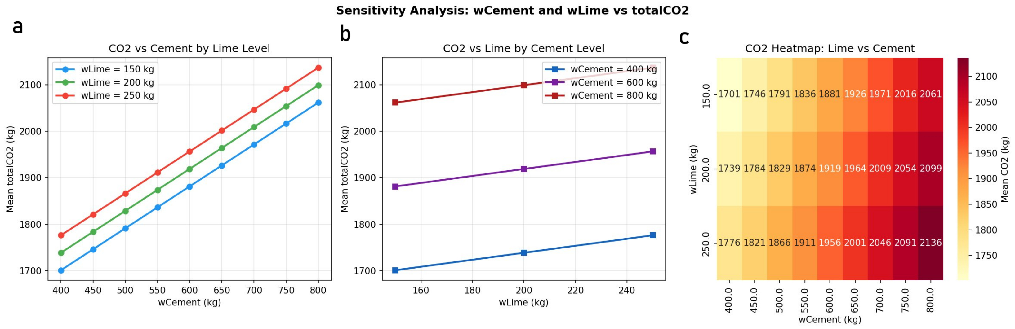
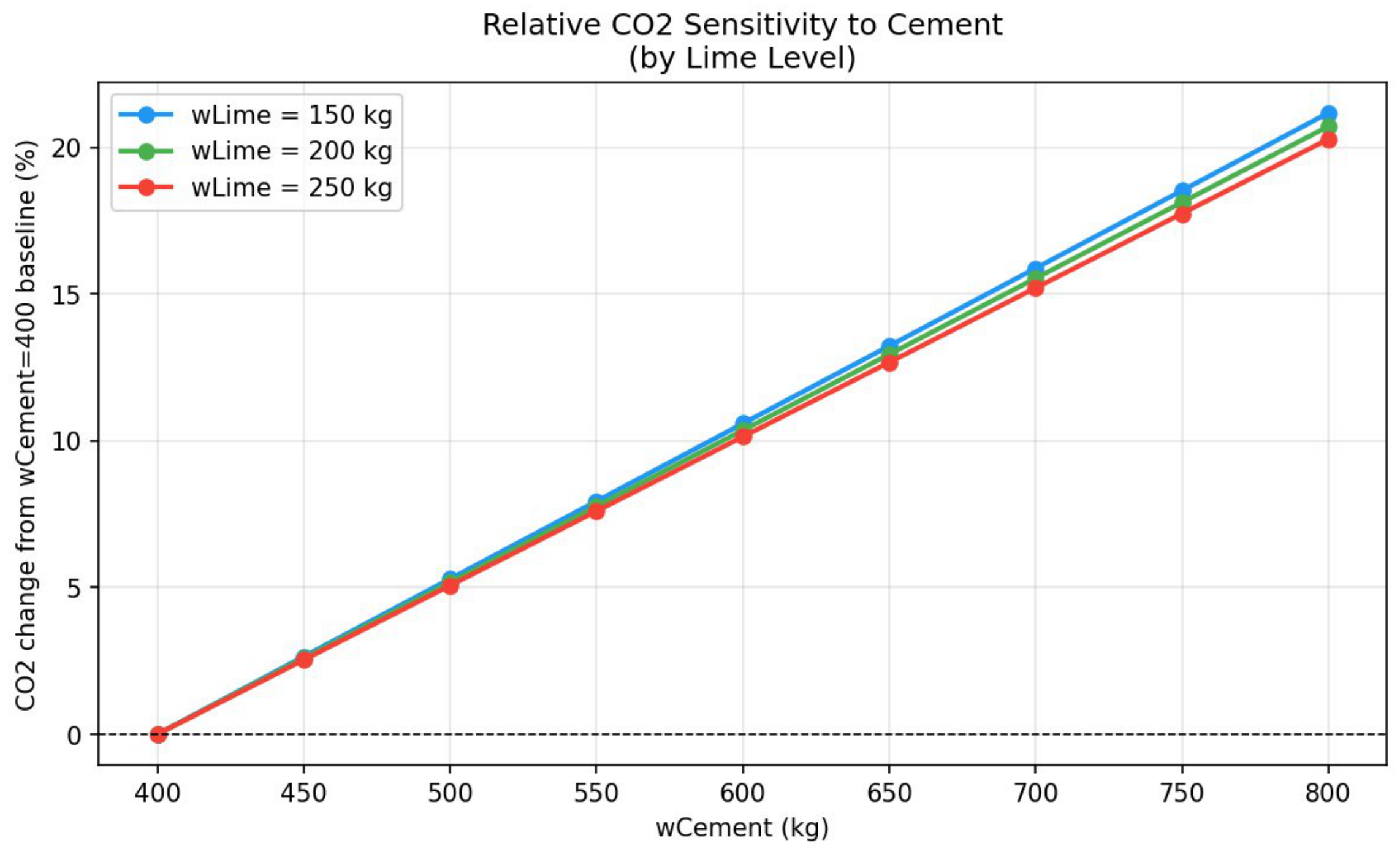
Lime and gypsum quantities were held fixed in the baseline simulation because the main experiment focused on controllable variation in cement use, electricity carbon intensity, autoclaving time, and production-capacity parameters. Appendix A shows that lime enters the emission model additively and linearly over the tested range, while gypsum was not varied and is therefore identified as a limitation for future plant-specific sensitivity analysis.

2.5. Machine-Learning Surrogate Modelling

We trained machine-learning surrogate models to approximate the outputs of the AAC discrete-event simulation. The surrogate models map production, resource, energy, and emission parameters to three response variables: total ${\mathrm{CO}}_2$e emissions, total production cost, and total actual production time. The complete simulation dataset generated from the experiment was divided into training and test subsets. We used 70% of the observations for model training and 30% for out-of-sample testing. The test set was not used during training. It provides an independent assessment of surrogate accuracy on unseen production configurations.

We trained four regression algorithms: a linear regressor, a Random Forest with 100 decision trees [27], a Gradient Boosting algorithm with 100 estimators [28], and an artificial neural network (ANN). These algorithms represent complementary surrogate classes. Linear regression provides an interpretable baseline. Random forest and Gradient Boosting capture nonlinear interactions between production parameters. The neural network provides a flexible nonlinear approximation model. The ANN comprises a series of dense layers and three outputs. The most accurate architecture was determined through trial and error by increasing the number of nodes and layers until good accuracy was achieved while preventing overfitting. 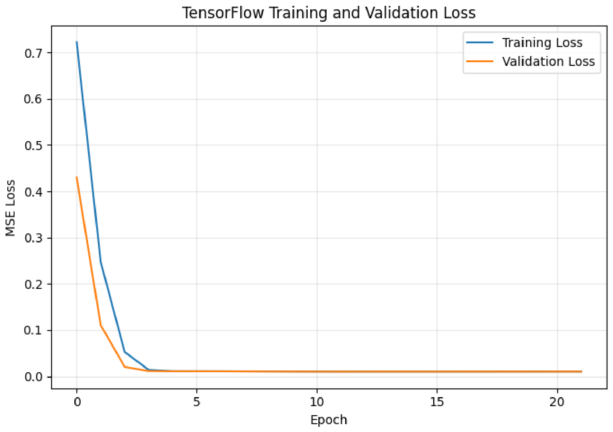The hidden layers consist of $32\times 16$ nodes. Dropout was not used because the training data were generated from a deterministic discrete-event simulation. The target variables were computed from controlled input parameters and explicit accounting equations, rather than from noisy experimental measurements. Consistent with this structure, the validation loss closely followed the training loss and showed no visible evidence of overfitting. The ANN architecture was selected through preliminary testing of candidate layer sizes rather than a formal hyperparameter search. Given the deterministic and structured nature of the simulation-generated data, this level of tuning was sufficient for stable convergence and high predictive accuracy.

The ReLU activation function was used for all nodes in the hidden layers [29]. The Adam optimization algorithm was used to fit the weights of the nodes [30]. A learning rate of 0.00005 was chosen to balance learning speed and convergence stability. Early stopping was applied with patience = 10 and restoration of the best weights. Training stopped at epoch 14 out of a maximum of 100 epochs, indicating that the model stopped once validation performance no longer improved. The scikit-learn library was used for the implementation and training of the algorithms [31], except for the artificial neural network which was implemented using TensorFlow [32].

Model accuracy was evaluated using mean absolute error (MAE), mean squared error (MSE), root mean squared error (RMSE), and the coefficient of determination $R^2$. For observed outputs $y_i$, predicted outputs ${\widehat{y}}_i$, sample mean $\overline{y}$, and test-set size n, the metrics are defined as

$$\mathrm{MAE}={\displaystyle \frac{1}{n}}{\displaystyle \sum _{i=1}^n}|y_i-{\widehat{y}}_i|.$$

(27)

$$\mathrm{MSE}={\displaystyle \frac{1}{n}}{\displaystyle \sum _{i=1}^n}{(y_i-{\widehat{y}}_i)}^2.$$

(28)

$$\mathrm{RMSE}=\sqrt{{\displaystyle \frac{1}{n}}\sum _{i=1}^n{(y_i-{\widehat{y}}_i)}^2}.$$

(29)

$$R^2=1-{\displaystyle \frac{{\sum }_{i=1}^n{(y_i-{\widehat{y}}_i)}^2}{{\sum }_{i=1}^n{(y_i-\overline{y})}^2}}.$$

(30)

Lower MAE, MSE, and RMSE indicate smaller prediction errors. Higher $R^2$ indicates stronger agreement between predicted and simulated outputs. Figure 2 shows that the training and validation losses decrease rapidly and then stabilize at low values. The close agreement between the two curves indicates stable training with no visible divergence between training and validation error. The training loss starts at approximately 0.72, while the validation loss starts at approximately 0.43. Both losses approach near-zero values by epoch 5 and then stabilize at a low MSE of approximately 0.01. This pattern indicates rapid learning of the dominant input–output structure in the simulation-generated dataset.

The validation loss remains close to the training loss throughout training. This behaviour provides no evidence of overfitting. The slightly lower validation loss during the early epochs is not problematic. It can occur when the validation subset is easier to predict, or when validation is evaluated under inference-mode settings rather than training-mode settings. This distinction is relevant for models using normalization layers, since batch-normalized networks can behave differently during training and inference. The small residual plateau after epoch 5 is consistent with the remaining prediction error observed in the actual-versus-predicted plots.

Table 10. Test-set performance metrics for total ${\mathrm{CO}}_2$e emissions.

Model	MAE	MSE	RMSE	${\mathit{R}}^2$
Random Forest	$7.87\times {10}^{-12}$	$1.15\times {10}^{-22}$	$1.07\times {10}^{-11}$	1.0000
Gradient Boosting	1.4143	3.1404	1.7721	0.9999
Linear Regression	63.33	7516.68	86.70	0.9693
Neural Networks	65.31	7571.50	87.01	0.9691

,

Table 11. Test-set performance metrics for total production cost.

Model	MAE	MSE	RMSE	${\mathit{R}}^2$
Random Forest	$6.24\times {10}^{-15}$	$3.55\times {10}^{-28}$	$1.88\times {10}^{-14}$	1.0000
Linear Regression	$7.19\times {10}^{-14}$	$9.64\times {10}^{-27}$	$9.82\times {10}^{-14}$	1.0000
Gradient Boosting	$4.45\times {10}^{-3}$	$3.80\times {10}^{-5}$	$6.17\times {10}^{-3}$	1.0000
Neural Networks	0.9723	1.4440	1.2017	1.0000

and

Table 12. Test-set performance metrics for total actual production time.

Model	MAE	MSE	RMSE	${\mathit{R}}^2$
Linear Regression	$6.30\times {10}^{-14}$	$4.77\times {10}^{-27}$	$6.91\times {10}^{-14}$	1.0000
Random Forest	$2.40\times {10}^{-13}$	$1.28\times {10}^{-25}$	$3.58\times {10}^{-13}$	1.0000
Gradient Boosting	$6.22\times {10}^{-6}$	$4.84\times {10}^{-11}$	$6.96\times {10}^{-6}$	1.0000
Neural Networks	0.2800	0.1203	0.3468	0.9999

report test-set performance for the three response variables. The surrogate models reproduced the simulation outputs with high accuracy on the held-out test set. Random forest achieved the lowest error for total ${\mathrm{CO}}_2$e emissions and total production cost. Linear regression achieved the lowest error for total actual production time, indicating that this response is nearly linear over the explored design space. Gradient Boosting also provided strong predictive performance across all outputs. The neural network achieved high $R^2$ values but larger absolute errors than the other models for these structured simulation-derived targets.

The near-perfect accuracy reflects the deterministic structure of the generated dataset. Total cost, total ${\mathrm{CO}}_2$e emissions, and total actual time are computed from controlled simulation inputs and explicit accounting equations. The surrogate models therefore learn stable input–output mappings rather than noisy empirical relationships. This result supports their use as fast emulators for optimization and scenario analysis. The surrogate models do not replace validation with physical production data. They provide a computational layer for exploring the simulated design space and identifying high-performing AAC production strategies for further evaluation. Because the targets are deterministic functions of the simulated inputs and explicit accounting equations, the surrogate is intended to emulate the full simulation-accounting pipeline at low computational cost rather than to infer a noisy empirical law.

2.6. Straight-Through Estimator Optimization

After training the artificial neural network surrogate model, we used it as a differentiable proxy for the AAC discrete-event simulation. The surrogate maps each candidate production configuration to three predicted outputs: total ${\mathrm{CO}}_2$e emissions, total production cost, and total actual production time. This enables gradient-based optimization without repeatedly executing the full simulation.

The optimization problem includes discrete input parameters. Examples include autoclaving time, mould quantity, storage size, traverse speed, and autoclave quantity. These variables take values from finite sets defined in the experiment. Standard gradient descent cannot be applied directly to hard discrete choices. We therefore used a straight-through estimator (STE), which allows hard selections in the forward pass while passing approximate gradients during backpropagation [14].

For a given candidate configuration, the surrogate predicts the normalized outputs ${\widehat{y}}_{{\mathrm{CO}}_2}^{*}$, ${\widehat{y}}_{\mathrm{cost}}^{*}$, and ${\widehat{y}}_{\mathrm{time}}^{*}$. The optimization minimizes the weighted objective

$$\mathcal{L}=\alpha {\widehat{y}}_{{\mathrm{CO}}_2}^{*}+\beta {\widehat{y}}_{\mathrm{cost}}^{*}+\gamma {\widehat{y}}_{\mathrm{time}}^{*}+\sigma P.$$

(31)

Here, $\alpha$, $\beta$, and $\gamma$ are user-defined objective weights with

$$\alpha +\beta +\gamma =1,$$

(32)

and $\sigma$ is a parameter which determines the weight of enforced penalties. The gradient-based optimization procedure was selected because the trained artificial neural network provides a differentiable surrogate of the AAC simulation. This allows the optimizer to evaluate many candidate production strategies at low computational cost, without repeatedly executing the full discrete-event factory model. The approach is well suited to the present problem because the objective combines multiple predicted outputs, including ${\mathrm{CO}}_2$e emissions, production cost, and production time. Once these outputs are approximated by a differentiable surrogate, gradients can be used to efficiently identify operating configurations that improve the weighted objective.

The production design space includes both nonlinear relationships and discrete decision variables. Nonlinearities arise from interactions among process duration, energy demand, material use, and emission factors. Discreteness arises because several operating variables can only take finite admissible values, including autoclaving time, mould quantity, storage capacity, traverse speed, and autoclave quantity. Standard gradient descent cannot directly optimize such hard discrete choices. We therefore used a straight-through estimator (STE). In the forward pass, the optimizer selects valid discrete parameter values from the admissible set. During backpropagation, gradients are passed through the underlying soft probability representation of each choice. This formulation preserves feasible production settings while enabling gradient-based optimization over a discrete manufacturing design space.

Discrete-Choice Straight-Through Estimator

Although several output variables are computed deterministically once a simulation run is completed, the full AAC production model is not a simple closed-form analytical function of the input parameters. The discrete-event simulation includes finite-capacity resources, routing logic, queues, waiting times, and discrete production decisions. These mechanisms determine operational outputs such as production time, resource use, and process-level energy demand before the emission and cost equations are applied. Therefore, direct analytical optimization of the accounting equations alone would not capture the full simulation-accounting pipeline.

Although Random Forest and linear regression achieved the smallest test errors for some outputs, we used the ANN in the optimization stage because it provides a differentiable surrogate compatible with the straight-through estimator. The ANN was therefore selected on methodological grounds rather than solely on predictive rank. Each discrete decision variable was represented by a vector of learnable logits. At each optimization step, the logits were transformed into softmax probabilities. The forward pass selected a hard discrete value using the largest probability. The backward pass used the soft probabilities to propagate gradients to the logits. This makes the optimization differentiable while preserving valid discrete decisions in the forward model.

The ANN surrogate was used because it provides a differentiable approximation of this complete pipeline. This differentiability enables gradient-based optimization of the weighted objective and allows the straight-through estimator to handle discrete production variables. During the forward pass, the optimizer selects valid discrete values from the admissible production settings. During backpropagation, gradients are passed through the corresponding soft probability representation. Thus, the ANN layer is not intended to replace known emission or cost equations. Its role is to convert a discrete and non-differentiable simulation workflow into a differentiable surrogate that can be optimized efficiently.

For each discrete parameter, the optimizer assigns a probability to every admissible value. During the forward pass, the model selects the value with the highest probability and evaluates the surrogate using this hard choice. During backpropagation, the straight-through estimator passes gradients through the underlying probability vector, which allows gradient-based optimization despite the discrete design space [14]. Let $\mathbf{p}$ be the softmax probability vector and let ${\mathbf{e}}_{\mathrm{hard}}$ be the one-hot vector associated with the selected value. The STE representation is

$$\tilde{\mathbf{e}}={\mathbf{e}}_{\mathrm{hard}}-\mathrm{stop}\text{\_}\mathrm{gradient}\left(\mathbf{p}\right)+\mathbf{p}.$$

(33)

The selected parameter value is

$$x=\sum _j{\tilde{e}}_j{v}_j,$$

(34)

where $v_j$ denotes the admissible values of the parameter. For example, autoclavingTime is selected from $\{50,80,110,140\}$ min. The softmax temperature was set to $\tau =0.75$. This value provides a practical balance between exploration and discrete selection. Lower temperatures produce sharper choices. Higher temperatures keep the probability distribution smoother and increase exploration. Here, the STE implementation used a single softmax temperature, $\tau =0.75$, for both the forward discrete selection and the backward gradient approximation. We did not tune separate forward and backward temperatures, ${\tau }_f$ and ${\tau }_b$, because the present optimization problem involved a relatively small finite design space and deterministic surrogate outputs. The single-temperature formulation provided stable optimization behaviour while keeping the implementation transparent and reproducible. Decoupling ${\tau }_f$ and ${\tau }_b$ may improve performance in larger or more complex discrete optimization settings, but benchmarking alternative STE temperature schemes was outside the scope of this study. Future work should evaluate whether separate forward and backward temperatures improve convergence, robustness, or solution quality for plant-specific AAC optimization problems. The STE implementation and optimization study was conducted using Tensorflow [32].

3. Results

3.1. Data Exploration and Feature Importance

The Section 3 first characterizes the simulation-generated dataset and identifies the main drivers of model outputs. We then evaluate how different optimization priorities affect predicted ${\mathrm{CO}}_2$e emissions, production cost, and production time. Finally, we examine the selected operating settings behind these outcomes to identify practical levers for lower-carbon AAC production. Together, these analyses connect the input design space, surrogate-model behaviour, and optimized production strategies.

We begin by examining the simulation dataset using correlation analysis and Random Forest feature importance. Reported ${\mathrm{CO}}_2$e and cost values correspond to one completed simulated production run, and production time denotes the total completion time of that run. The correlation matrix evaluates pairwise linear associations between variables. Correlation coefficients range from $-1$ to 1, where values near 1 indicate strong positive association, values near $-1$ indicate strong negative association, and values near 0 indicate weak linear association [33]. Figure 3a shows the correlation matrix for the raw input parameters and output variables. The design variables show weak correlations with each other, which confirms that the simulation varied the main inputs independently. The total ${\mathrm{CO}}_2$e emissions, total production cost, and total actual production time show strong positive associations with autoclaving time. They also show strong positive associations with each other. This result is consistent with the production logic of AAC manufacturing. Longer autoclaving increases processing time and energy demand, which directly affects emissions and cost.

Figure 3b shows the Random Forest feature-importance scores [34]. Autoclaving time is the dominant predictor, contributing approximately 67% of total importance. Electricity emission factor is the second most influential variable, contributing approximately 27%. Cement mass contributes approximately 5%. Storage capacity, mould quantity, autoclave traverse speed, and the number of autoclaves show negligible importance under the tested conditions.

These results provide a clear interpretation of the simulation dataset. Output variation is driven mainly by autoclaving time, electricity carbon intensity, and cement use. These variables correspond to the main mechanisms in the model: steam-curing duration, electricity-related emissions, and material-related emissions. The analysis therefore identifies the primary levers for surrogate modelling, scenario analysis, and optimization.

3.2. Sustainable, Cost-Effective, and Time-Efficient AAC Production Strategies

We consider seven representative strategies defined as follows: balanced strategy, with equal priority assigned to carbon footprint, cost, and time $(\alpha =\beta =\gamma =1/3)$; carbon-priority strategy, with full priority assigned to carbon footprint $(\alpha =1)$; cost-priority strategy, with full priority assigned to cost $(\beta =1)$; time-priority strategy, with full priority assigned to production time $(\gamma =1)$; carbon–cost strategy, with equal priority assigned to carbon footprint and cost $(\alpha =\beta =0.5,\gamma =0)$; carbon–time strategy, with equal priority assigned to carbon footprint and production time $(\alpha =\gamma =0.5,\beta =0)$; and cost–time strategy, with equal priority assigned to cost and production time $(\beta =\gamma =0.5,\alpha =0)$.

The seven optimization strategies use predefined weights to represent different decision preferences, including carbon-priority, cost-priority, time-priority, and balanced operating objectives. These weights are therefore not unique or fully objective; they provide interpretable scenarios for comparing how different priorities influence the selected AAC production strategy. The weighted formulation is useful for decision support because it converts the multi-objective problem into a single scalar objective, but it does not replace a full Pareto analysis.

Before comparing the optimization outcomes, we summarize the seven decision strategies used in the analysis. Each strategy assigns a different weight to ${\mathrm{CO}}_2$e emissions, production cost, and production time, allowing the optimizer to evaluate single-objective, dual-objective, and balanced production priorities.

Table 13. Optimization strategies evaluated in Section 3.2.

Strategy	Carbon Weight $\mathit{\alpha }$	Cost Weight $\mathit{\beta }$	Time Weight $\mathit{\gamma }$
Balanced	$1/3$	$1/3$	$1/3$
Carbon priority	1	0	0
Cost priority	0	1	0
Time priority	0	0	1
Carbon–cost	$0.5$	$0.5$	0
Carbon–time	$0.5$	0	$0.5$
Cost–time	0	$0.5$	$0.5$

summarizes the coefficients considered for each of the considered seven strategies.

We compare the predicted outcomes obtained under seven decision strategies. Each strategy assigns a different priority to carbon footprint, production cost, and production time. This weighting approach converts the multi-objective problem into a single composite objective, while recognizing that the selected solution depends on the assigned priorities. Figure 4 summarizes the ranked ANN-predicted optimal outcomes.

Figure 4a shows the ANN-predicted ${\mathrm{CO}}_2$e emissions. The Carbon + Cost and Carbon Priority strategies produce the lowest predicted emissions, approximately 1291.82 and 1291.83 kg ${\mathrm{CO}}_2$e, respectively. The Cost Priority strategy gives an intermediate value of approximately 1555.96 kg ${\mathrm{CO}}_2$e, followed by the Balanced and Carbon + Time strategies, both near 1651 kg ${\mathrm{CO}}_2$e. The Cost + Time strategy yields a substantially higher value of approximately 2188.18 kg ${\mathrm{CO}}_2$e, while the Time Priority strategy produces the highest predicted emissions, approximately 3093.30 kg ${\mathrm{CO}}_2$e. This pattern indicates that strategies with explicit carbon weighting substantially reduce predicted emissions, whereas prioritizing time alone shifts the solution toward a much higher-carbon operating regime.

Figure 4b shows the ANN-predicted production cost. The Carbon + Cost, Carbon Priority, and Cost Priority strategies produce the lowest predicted costs, with values near 412 currency units. The Balanced, Carbon + Time, and Cost + Time strategies form an intermediate group near 460 currency units. The Time Priority strategy gives the highest predicted cost, approximately 695.22 currency units. Therefore, the ranking of cost follows a similar structure to the emission outcome: strategies that include carbon or cost objectives remain in the lower-cost region, whereas the Time Priority strategy substantially increases predicted cost. This result is consistent with the reworked trade-off formulation, in which shorter or more accelerated production can require higher process-intensification cost.

Figure 4c shows the ANN-predicted reworked production time. The Time Priority strategy yields the lowest predicted reworked time, approximately 209.23 min. The Cost + Time, Carbon + Time, and Balanced strategies follow closely, with predicted times near 212.45–212.46 min. In contrast, the Cost Priority, Carbon Priority, and Carbon + Cost strategies produce the highest predicted reworked times, approximately 237.62 min. This ranking indicates that strategies emphasizing time select faster configurations, while strategies emphasizing carbon or cost accept longer reworked production times. Therefore, the reworked formulation introduces a clearer cost–time trade-off than the original simulation output, where production time was largely determined by autoclaving duration and fixed baseline process times.

The strategy comparison shows that carbon footprint and cost are highly sensitive to the assigned decision priorities. The lowest-emission and lowest-cost strategies are obtained when carbon and/or cost objectives are included explicitly. By contrast, prioritizing time alone leads to the highest predicted ${\mathrm{CO}}_2$e emissions and cost. Next, we compare the selected values of two influential environmental inputs across the seven decision strategies: electricity emission factor and cement mass. Across the optimized configurations, autoclaving time remained a dominant driver of production-time behaviour. Therefore, Figure 5 focuses on electricity carbon intensity and cement use, which directly influence the predicted ${\mathrm{CO}}_2$e and cost outcomes. The comparison complements the outcome-level analysis by showing how the decision strategies change the underlying operating choices that generate the predicted trade-offs.

Figure 5a shows the selected electricity emission factor. The Balanced, Carbon + Cost, Carbon + Time, and Carbon Priority strategies select the lowest electricity emission factor, 0.05 kg ${\mathrm{CO}}_2$e/kWh. The Cost Priority strategy selects an intermediate value of 0.43 kg ${\mathrm{CO}}_2$e/kWh. The Cost + Time and Time Priority strategies select the highest value, 0.81 kg ${\mathrm{CO}}_2$e/kWh. This pattern explains the higher ${\mathrm{CO}}_2$e emissions observed for the time-oriented strategies in Figure 4a. When the objective emphasizes time, the optimizer can move toward configurations with higher electricity carbon intensity, whereas strategies with explicit carbon weighting select lower-carbon electricity.

Figure 5b shows the selected cement mass. The Carbon + Cost, Carbon Priority, and Cost Priority strategies select the lowest cement mass, 400 kg. In contrast, the Balanced, Carbon + Time, Cost + Time, and Time Priority strategies select the highest cement mass, 800 kg. Since cement contributes directly to material-related emissions, the higher cement selections help explain why several mixed or time-oriented strategies produce larger predicted emissions. These results should not be interpreted as recommending higher cement use for sustainability. Rather, they reflect the behaviour of the weighted composite objective over a discrete feasible design space.

Together, Figure 4 and Figure 5 show that the decision strategy affects both the predicted outcomes and the operating choices that produce them. Carbon-weighted strategies reduce emissions primarily by selecting low-carbon electricity and lower cement use. Cost-weighted strategies also favour lower cement use and lower predicted cost. Time-oriented strategies reduce reworked production time but can select higher electricity carbon intensity and higher cement mass, leading to larger predicted ${\mathrm{CO}}_2$e emissions and cost. These findings identify electricity sourcing, cement intensity, and the assumed cost of accelerated curing as key levers controlling the sustainability trade-offs in the AAC production model.

4. Discussion

This study developed a hybrid simulation-optimization framework for sustainable AAC production. The framework combines a discrete-event factory model, stage-based ${\mathrm{CO}}_2$e and cost accounting, machine-learning surrogate models, and gradient-based optimization. The simulation represents the main AAC production stages, including mix preparation, mould pouring and rising, cutting, autoclaving, unloading, and product handling. Relative to the public AnyLogic AAC example [20], we added stage-level energy and ${\mathrm{CO}}_2$e accounting, a cost model, parameter sweeps for large-scale dataset generation, and automated export of run-level outputs for surrogate training and optimization. This structure preserves the operational logic of AAC manufacturing while enabling large-scale scenario generation. The carbon model accounts for material-related emissions, electricity use, and thermal energy demand. This is consistent with previous AAC life-cycle evidence showing that cement and lime dominate upstream emissions, while steam generation for autoclaving remains a key factory-stage emission source [2]. By training surrogate models on approximately 116,640 simulated scenarios, the framework enables rapid prediction of ${\mathrm{CO}}_2$e emissions, production cost, and completion time across alternative operating strategies.

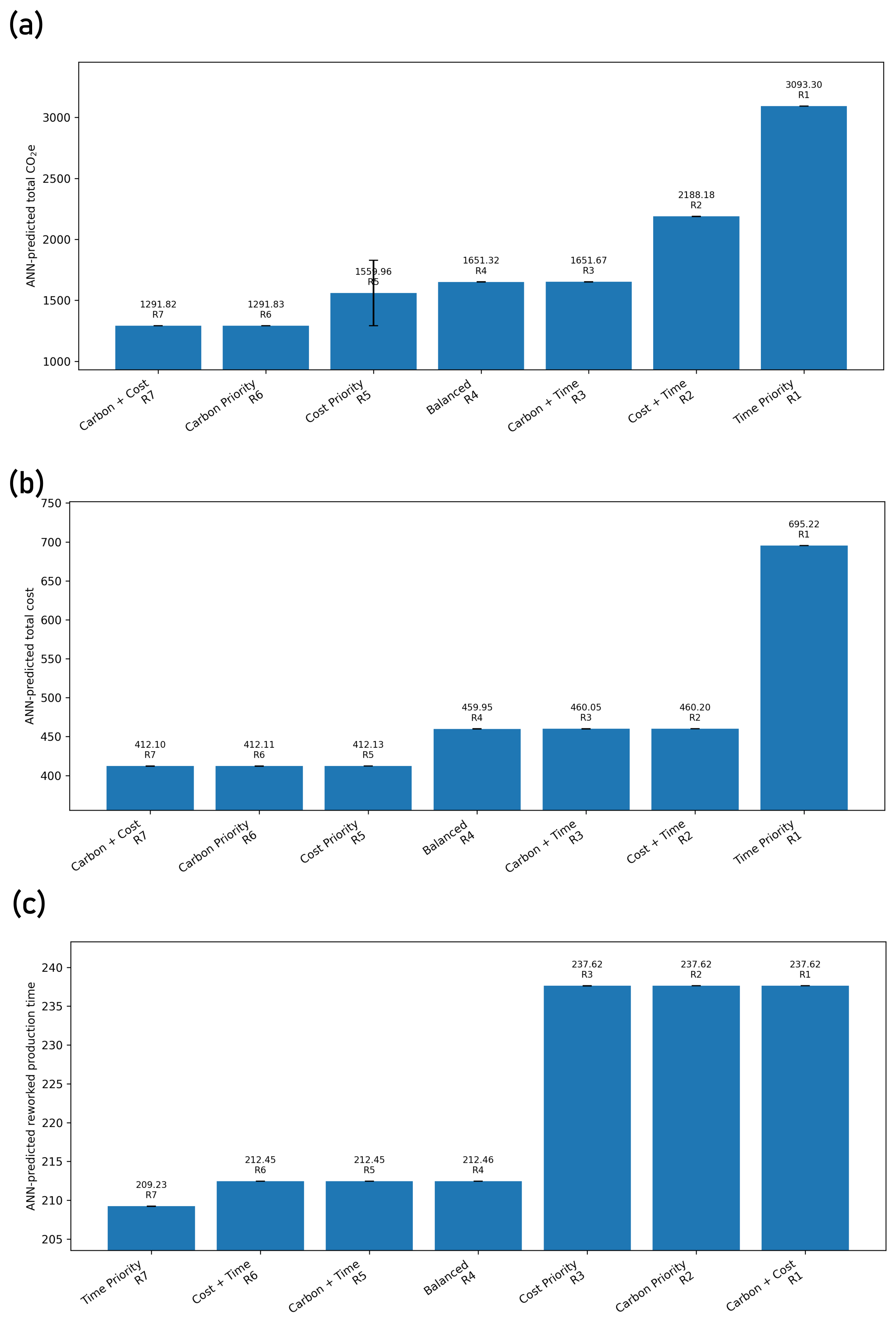
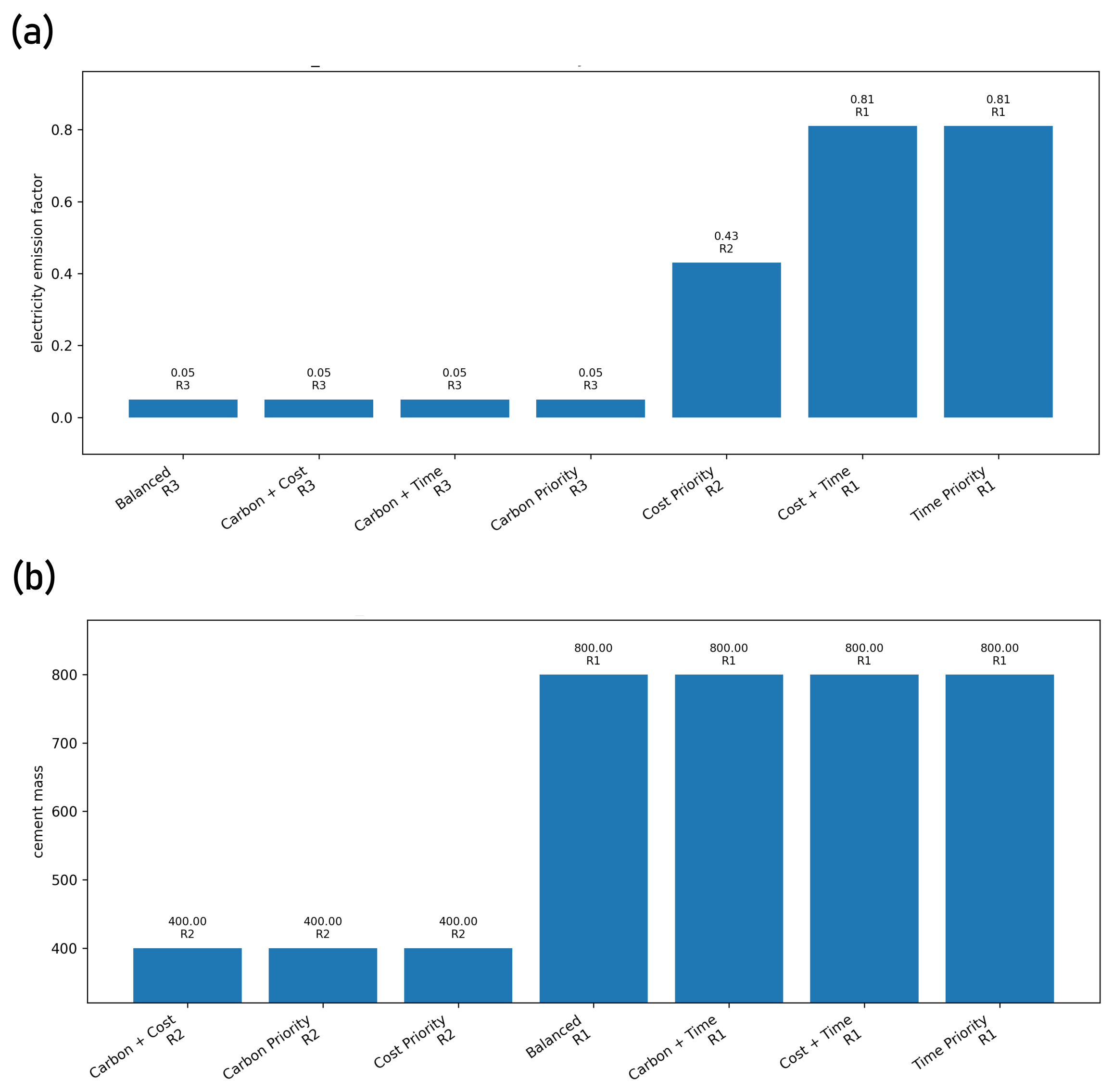
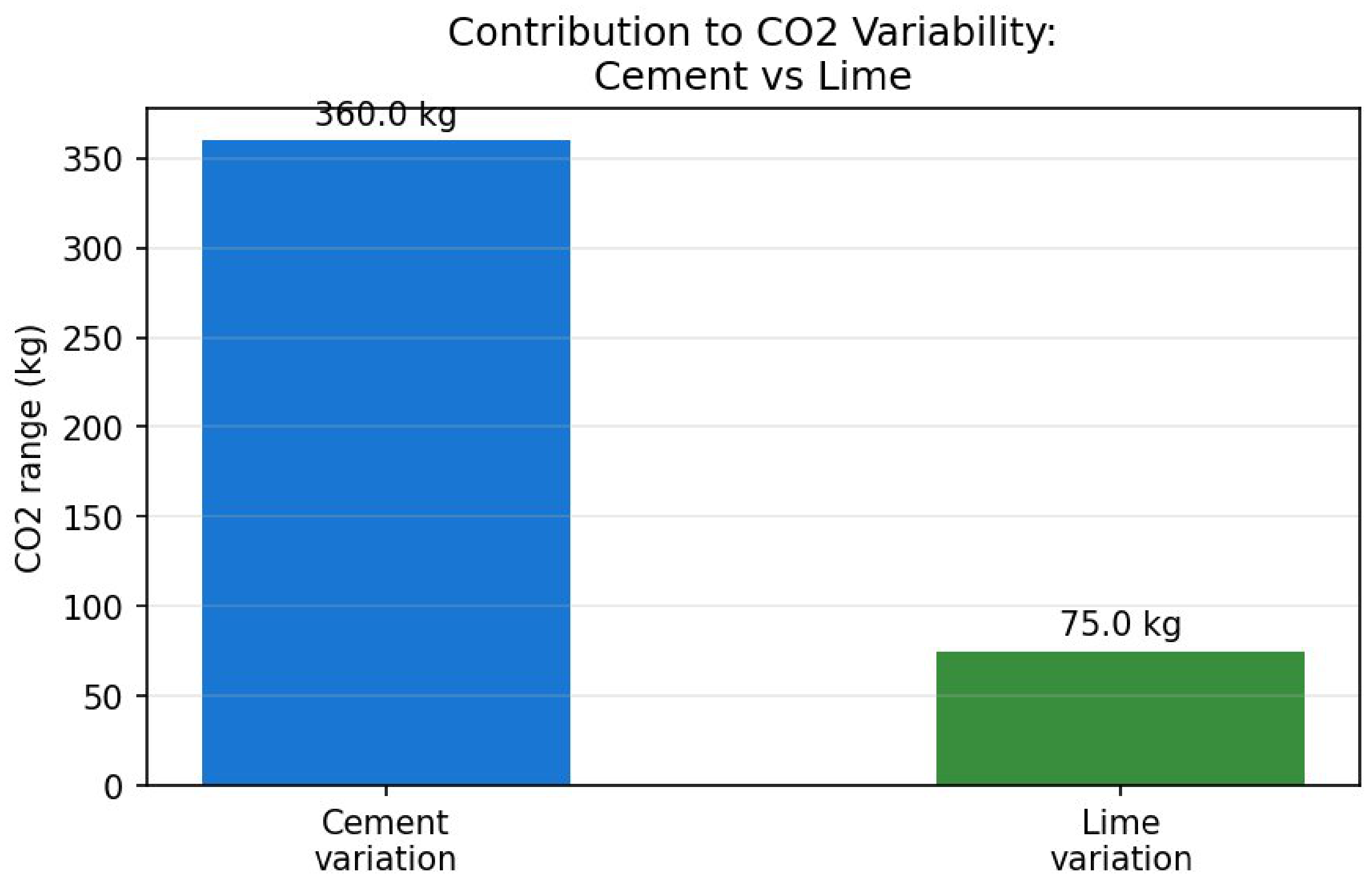
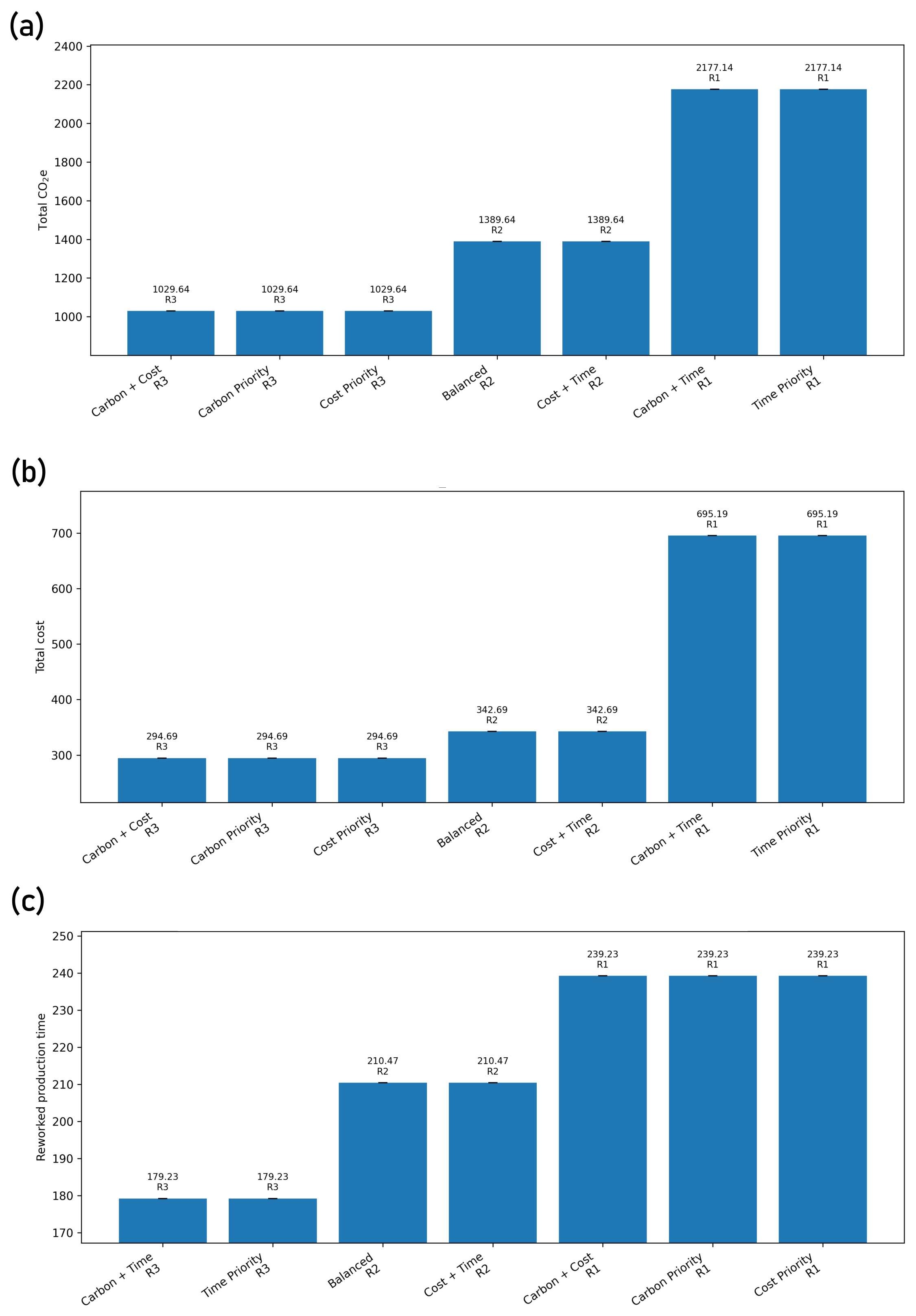
The results identify electricity carbon intensity, cement use, and the assumed cost of accelerated curing as the main levers governing the simulated AAC trade-offs. The Carbon + Cost and Carbon Priority strategies produced the lowest predicted ${\mathrm{CO}}_2$e emissions, approximately 1291.82 kg ${\mathrm{CO}}_2$e, and selected the lowest electricity emission factor, 0.05 kg ${\mathrm{CO}}_2$e/kWh. These strategies also selected the lowest cement mass, 400 kg, together with the Cost Priority strategy. In contrast, the Time Priority strategy achieved the shortest reworked production time but produced the highest predicted ${\mathrm{CO}}_2$e emissions and cost, reflecting the added burden associated with accelerated production. 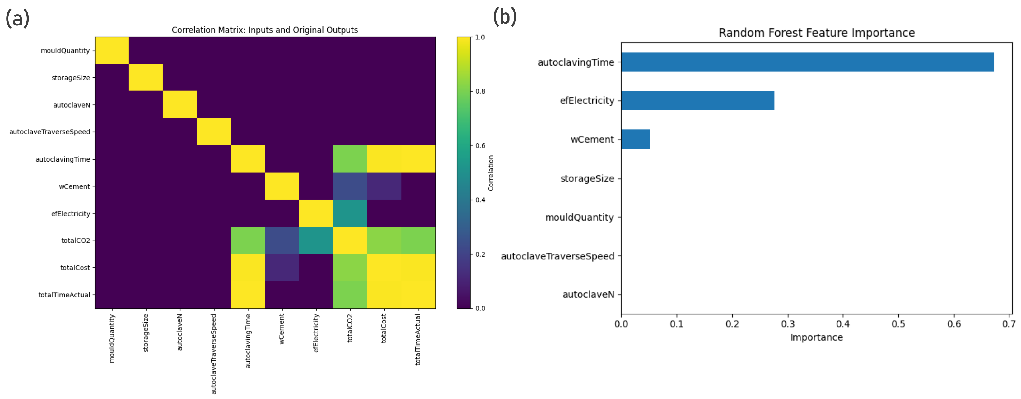Across the strategies, predicted ${\mathrm{CO}}_2$e emissions and cost varied more strongly than reworked production time, indicating that prioritizing time can substantially increase environmental and economic burden. The feature-importance and strategy analyses were consistent: autoclaving time, electricity carbon intensity, and cement use governed most of the variation in emissions, cost, and time. These findings suggest that AAC decarbonization should combine lower-carbon electricity or steam generation, careful management of autoclave operation, and reduction or substitution of carbon-intensive binders. The results also show that carbon- and cost-oriented strategies can reduce emissions without selecting the most time-intensive operating regime, supporting the need for practical guidelines that help manufacturers balance low-carbon production with operational feasibility. The ranking of optimal strategies was validated by a brute force search study (Figure A4).

Across all optimization strategies, the selected autoclaving time converged to the minimum admissible value of 50 min. This result should be interpreted in light of the current model assumptions. In the present framework, autoclaving time increases thermal-energy demand, electricity use, production cost, ${\mathrm{CO}}_2$e emissions, and completion time, but product-quality constraints such as strength development, density, curing completeness, and dimensional stability are not explicitly modelled. Therefore, longer autoclaving does not provide a compensating benefit in the objective function. Autoclaving time was retained as a decision variable because it is a central operational lever in AAC production and because the analysis tests whether longer curing durations are selected under different carbon, cost, time, and balanced priorities. The consistent selection of 50 min is therefore conditional on the simulated design space and should not be generalized to all AAC plants. Future plant-specific implementations should include curing-quality and mechanical-performance constraints, under which longer autoclaving times may be required or optimal.

A gradient-based optimization method was selected because the artificial neural network provides a differentiable surrogate of the AAC simulation. This allows rapid exploration of candidate production strategies without repeatedly executing the full discrete-event model. The production design space includes nonlinear relationships among energy use, process time, material use, and emissions, as well as discrete variables such as autoclaving time, mould quantity, storage capacity, traverse speed, and autoclave quantity. To handle these discrete choices, we used a straight-through estimator. The optimizer selects valid discrete values during the forward pass, while approximate gradients are passed through a soft probability representation during backpropagation. This preserves feasible production settings while enabling efficient gradient-based optimization.

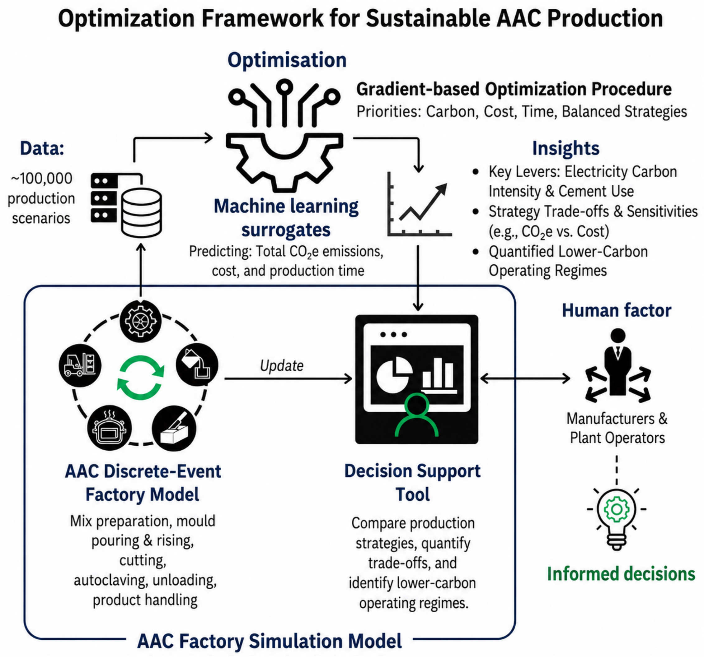
Figure 6 shows how the proposed framework can operate as a smart manufacturing layer for AAC production. The discrete-event model represents the main factory stages and generates 116,640 production scenarios. The surrogate models then learn fast mappings from operating settings to ${\mathrm{CO}}_2$e emissions, cost, and production time. Coupled with gradient-based optimization, this structure allows plant operators to compare carbon-, cost-, time-, and balanced strategies before changing factory conditions. In this sense, the framework provides a digital twin-like decision-support tool for AAC manufacturing: it links process simulation, data-driven prediction, and optimization to identify lower-carbon operating regimes and update production policies as new plant data become available [35,36].

This study has a few limitations that should guide interpretation and future work. The simulation dataset covers a broad but finite design space, with particular emphasis on parameters that influence autoclaving because steam curing is one of the most energy-intensive factory operations in AAC production. Adding more operational variables, such as raw-material logistics, maintenance disruptions, worker schedules, product geometry, quality constraints, boiler efficiency, heat recovery, and site-specific energy systems, would require additional simulation runs to preserve surrogate-model accuracy. This is a standard limitation of simulation-based surrogate modelling, where higher-dimensional design spaces require denser sampling or adaptive experimental designs to maintain reliable prediction and optimization performance [37]. We focused on autoclaving because steam curing is one of the most energy-intensive factory operations in AAC production and has been identified as an important contributor in AAC life-cycle studies [2]. However, other stages may also affect emissions, cost, and throughput, especially when material preparation, lime grinding, transport, storage, downtime, or plant-specific fuel systems are included [2]. Heat recovery was not explicitly included in the present model because the public AAC factory simulation does not resolve plant-specific steam-system design, condensate recovery, boiler efficiency, heat-exchanger performance, or recovered-heat allocation. The current framework therefore represents thermal-energy demand directly through the rising and autoclaving stages. This is a limitation because heat recovery has been identified as an important AAC decarbonization lever. Including heat recovery would reduce the effective thermal-energy demand of steam curing and could change the optimal strategies by lowering the carbon penalty associated with autoclaving time. As a result, the relative importance of autoclaving time may decrease, while binder-related emissions from cement and lime may become more dominant. Future plant-specific implementations should include heat-recovery efficiency, boiler losses, condensate return, and recovered-heat reuse to evaluate this pathway quantitatively. The present framework should therefore be interpreted as a decision-support, focusing on optimizing the autoclaving process during AAC manufacturing, rather than a complete plant certification model.

This study shows that sustainable AAC manufacturing can be evaluated as part of a broader construction value chain. The proposed surrogate model provides a fast representation of factory-level emissions, cost, and production time. Future work will integrate this model into Modular Integrated Construction (MiC) supply chain frameworks to evaluate how manufacturing decisions interact with logistics, storage, assembly, and site-installation strategies. This extension is important because MiC performance depends on coordinated decisions across factories, transport fleets, and construction sites, and recent studies show that simulation and optimization can improve MiC supply-chain sustainability by reducing duration, cost, and carbon emissions [38]. A coupled AAC-MiC framework would allow decision makers to compare low-carbon production policies with supply-chain strategies and identify solutions that reduce emissions without shifting burdens from manufacturing to logistics or construction operations. The electricity emission factor was varied from 0.05 to 0.81 kg ${\mathrm{CO}}_2$e/kWh to represent different grid-carbon-intensity conditions. This provides a partial sensitivity analysis for one of the most important regional emission parameters. The results show that electricity carbon intensity strongly influences predicted ${\mathrm{CO}}_2$e emissions and can affect the attractiveness of strategies involving electricity-intensive or autoclaving-related operations. However, other emission factors and cost parameters, including heat emissions, cement, lime, aluminum, electricity price, heat price, and material unit costs, were held fixed using literature or database values. Therefore, the numerical results should be interpreted as conditional on these assumptions. Future plant-specific applications should include a broader sensitivity analysis using regional grid factors, local fuel mixes, boiler efficiency, site-specific energy tariffs, and actual material prices.

Finally, the present framework was developed using a public AnyLogic AAC factory model and simulation-generated production data. Therefore, the reported production times, energy consumption, ${\mathrm{CO}}_2$e emissions, and optimized operating strategies should be interpreted as model-based estimates rather than direct measurements from an industrial AAC plant. The study demonstrates the feasibility of integrating discrete-event simulation, emission and cost accounting, machine-learning surrogate modelling, and optimization into a unified decision-support workflow. However, validation against real factory operational data remains necessary before industrial deployment. Future work should calibrate and validate the model using plant-specific records, including measured cycle times, autoclave energy demand, throughput, material consumption, production cost, and site-specific emission factors. Such validation would allow the framework to better represent actual AAC manufacturing conditions and improve confidence in its use for operational decision making.

5. Conclusions

This study contributes a unified decision-support framework for sustainable AAC production by integrating discrete-event simulation, ${\mathrm{CO}}_2$e and cost accounting, machine-learning surrogate modelling, and gradient-based optimization into a single workflow. This integration is the main novelty of the work. It allows AAC production strategies to be tested computationally, translated into fast surrogate predictions, and optimized across carbon, cost, and time objectives before implementation in a physical factory. The proposed framework can be extended to AAC formulations based on alternative raw materials, such as fly ash, tailings, or recycled AAC powder, but it cannot be transferred without recalibration. Model migration would require updating the material masses, emission factors, cost parameters, curing requirements, and quality constraints associated with the alternative mix design. The discrete-event structure can remain largely unchanged, while the emission, cost, and performance modules should be recalibrated using formulation-specific and plant-specific data.

The results show that the optimization priority can meaningfully change predicted environmental performance. The carbon-priority strategy reduced predicted emissions to approximately 1855 kg ${\mathrm{CO}}_2$e, while the highest-emission strategies exceeded 2050 kg ${\mathrm{CO}}_2$e. This corresponds to an approximate reduction of 195 kg ${\mathrm{CO}}_2$e, or about 9–10%, across the tested strategies. In contrast, the cost spread was modest, about 19 currency units, and production time varied by only approximately 0.6 min under the modelled assumptions. These findings indicate that, within the simulated design space, lower-carbon AAC production can be achieved mainly through electricity carbon intensity, cement use, and autoclaving-related decisions, without large predicted penalties in production time.

Future work should extend the framework through plant-specific calibration and validation against real factory operational data. This includes comparing predicted production time, energy use, throughput, cost, and ${\mathrm{CO}}_2$e emissions with measured factory records. Such validation is necessary to assess the transferability of the surrogate models, refine site-specific assumptions, and support reliable deployment of the framework as an operational decision-support tool for AAC manufacturers.