A Pilot Study of SHAP-Interpreted Machine Learning for Pixel-Level Landslide Classification from High-Resolution DEM and Satellite Imagery

Abstract

Accurate delineation of current landslide extent is important for hazard assessment, sustainable watershed management, and disaster risk reduction in tectonically active mountainous regions. This study presents a pilot machine learning framework for pixel-level landslide classification in the Laonung (Laonong) Creek Watershed, southern Taiwan, using very high-resolution digital elevation model (DEM) derivatives and SPOT-6 multispectral imagery. Thirteen geomorphometric and spectral features, including slope, curvature, and six spectral indices derived from SPOT-6 bands, were extracted from 96 landslide-containing tiles within a pilot subregion of the watershed; no landslide-free tiles were included in model training or evaluation. Landslide annotations followed a geomorphic-unit delineation protocol in which optical imagery provided the primary evidence of current activity and DEM-derived hillshade supported boundary refinement. Three classifiers were evaluated using column-quartile spatially blocked four-fold cross-validation, with each fold comprising a geographically contiguous range of columns, to reduce spatial leakage: logistic regression (LR), random forest (RF), and XGBoost. All three models substantially outperformed the no-skill baseline for the resampled evaluation dataset (average precision, AP $=0.250$), achieving mean AP values of $0.854\pm 0.040$, $0.858\pm 0.033$, and $0.846\pm 0.035$ for LR, RF, and XGBoost, respectively. The convergence of linear and nonlinear model performance suggests that the dominant discriminatory signal is largely captured by relatively simple spectral and topographic predictors within this pilot dataset, rather than reflecting a general property of landslide classification. SHapley Additive exPlanations (SHAP) analysis across all four spatial folds identified SPOT-6 Band 3 (Red) as the dominant predictor in every fold, with NDVI a robust secondary predictor, consistent with the spectral characteristics of fresh bare-soil landslide surfaces and with the optical cues used in the annotation protocol. The results are interpreted in the context of the pilot dataset’s limited spatial extent, the resampled class distribution used for model evaluation, and unquantified label uncertainty. This study provides a transferable methodological baseline for future, larger-scale landslide classification analysis in the Laonung Creek Watershed and highlights the potential contribution of spatially explicit landslide mapping to sustainability-oriented disaster management.

1. Introduction

Taiwan’s mountainous topography, abundant rainfall, and frequent earthquakes make it highly susceptible to landslides, resulting in repeated and sometimes severe mass-movement events [1,2,3,4,5]. The Laonung (Laonong) Creek Watershed in southern Taiwan is particularly susceptible and has experienced multiple large-scale landslide events associated with typhoons and earthquakes in recent decades [6,7,8,9,10,11,12,13,14]. Timely and accurate mapping of current landslide extent is therefore important for hazard assessment, disaster response, and long-term monitoring of watershed dynamics [15]. Beyond immediate hazard response, reliable landslide mapping underpins sustainable watershed management and disaster risk reduction, informing land-use planning and mitigation decisions that sustain mountain communities and downstream water resources.

Remote sensing-based landslide mapping has advanced substantially with the increasing availability of high-resolution digital elevation models (DEMs) and multispectral satellite imagery [16,17,18,19,20,21]. DEM-derived variables such as slope, curvature, and hillshade provide geomorphometric information relevant to terrain instability, whereas optical imagery provides spectral information related to bare soil exposure and vegetation disturbance associated with recent mass movement [22]. The complementary roles of topographic and optical data have motivated many fusion-based mapping approaches, and previous studies have reported improved classification performance when both data types are used together rather than separately [23,24,25,26,27,28].

Machine learning approaches are now commonly used for landslide susceptibility mapping and classification. Among these methods, random forest and gradient-boosting models have frequently demonstrated reliable predictive performance under a wide range of geological and climatic conditions [29,30,31,32,33,34]. Despite this progress, four methodological gaps recur in the literature. First, random or stratified random splitting of spatially correlated data can produce optimistic performance estimates because of spatial leakage between training and test sets, a problem that has been shown to inflate reported accuracy in geospatial classification tasks [35,36,37,38,39]. Second, many machine learning models trained on geospatial features provide limited insight into which variables are most strongly associated with model predictions, thereby constraining interpretability [40,41,42,43,44]. Third, many studies rely on large pre-existing landslide inventories without explicitly addressing the particular challenges of expert-annotated, geomorphically interpreted datasets, in which label boundaries are intended to represent the extent of physical units rather than spectral contrast alone [45,46,47]. Fourth, linear baselines are not always benchmarked against nonlinear ensemble methods in high-resolution landslide classification, making it difficult to assess whether model complexity contributes meaningful discriminatory power beyond what simple linear predictors already capture.

In the context of remote sensing-based landslide mapping, object-based image analysis (OBIA) represents an alternative approach that groups spatially adjacent pixels into homogeneous segments before classification, potentially capturing shape and texture context that per-pixel methods ignore [24,48]. However, OBIA requires segment scale parameters that are difficult to optimize without prior knowledge of landslide size and morphology, and segment boundaries may not align with the geomorphic unit boundaries delineated by expert annotators. In the present study, a pixel-level framework was adopted because the ground-truth labels are stored as binary pixel masks, pixel-level feature engineering combined with SHAP analysis provides straightforward per-feature attribution, and the spatial context limitation of pixel-level classification is explicitly addressed in the companion deep learning study [49], which applies U-Net semantic segmentation to the same annotated dataset.

This study addresses these issues in a pilot-study setting through three main contributions. First, we apply spatially blocked cross-validation to obtain more conservative performance estimates for a geographically constrained pilot dataset. Second, we employ SHAP (SHapley Additive exPlanations) analysis [50] to examine how geomorphometric and spectral features contribute to model predictions, thereby providing an interpretable summary of model behavior. Third, we document a quality-control annotation protocol, rather than a novel methodological advance, in which landslide delineations are based on geomorphic-unit boundaries rather than spectral patch edges. SPOT-6 optical imagery is used as the primary evidence of current activity, and a high-resolution DEM provides supporting context for boundary refinement; this protocol promotes annotation consistency and transparency within the present pilot dataset.

We explicitly frame this work as a pilot study. The annotated dataset comprises 128 tiles, of which 96 contain landslides, concentrated in a four-row subregion of the Laonung Creek Watershed. Therefore, the results should not be interpreted as representative of the full watershed or as a definitive benchmark. In addition, because model training and evaluation were conducted on a resampled pixel distribution within the annotated tiles, the reported metrics should be interpreted within this experimental setting rather than as direct estimates of full-watershed deployment performance. As annotation progresses toward the full 2048-tile dataset, the model will encounter terrain types, landslide morphologies, and vegetation conditions beyond those represented in the present pilot subregion. Model performance may therefore decline before it improves as the training data expand into less-represented parts of the watershed. Transferability of the present framework to new spatial extents requires consistent DEM resolution and derivative computation, consistent sensor configuration and spectral band availability, and use of the same annotation protocol. Within these limits, this study provides a transferable pilot baseline for subsequent larger-scale landslide classification analysis in the Laonung Creek Watershed.

2. Study Area

The Laonung (Laonong) Creek Watershed lies within Kaohsiung City in southern Taiwan, where it conveys runoff from the southern part of the Central Mountain Range into the Kaoping (Gaoping) River system. The Laonung Creek watershed is a large mountainous basin with a reported drainage area of approximately 1370 km² and strong topographic relief, rising from low-elevation downstream areas to more than 3900 m in the upper watershed [51,52]. The basin is underlain mainly by slate, sandstone–shale, and related metamorphic to sedimentary formations arranged along a predominantly northeast–southwest structural trend [51,52]. The climate is humid, and rainfall is strongly seasonal, with mean annual rainfall in the mapped Laonung sector reported to be about 2601 mm at Fuhsing and 3406 mm at Hsiaokuanshan [52]. The watershed has experienced numerous large landslide events triggered by typhoons and earthquakes, making it an appropriate study area for landslide mapping and monitoring in Taiwan [6,7,8,9]. The watershed is predominantly forested, with dense subtropical and montane vegetation covering most hillslopes. Landslide scars are typically characterized by bare soil, exposed weathered rock, or colluvium with little or no vegetation cover, creating strong spectral contrast with the surrounding forested terrain that is used by the classification framework presented in this study. A representative example of the terrain and land cover at the tile level, including the SPOT-6 natural-color composite and DEM-derived hillshade, is presented with the annotation workflow in Section 3.2.

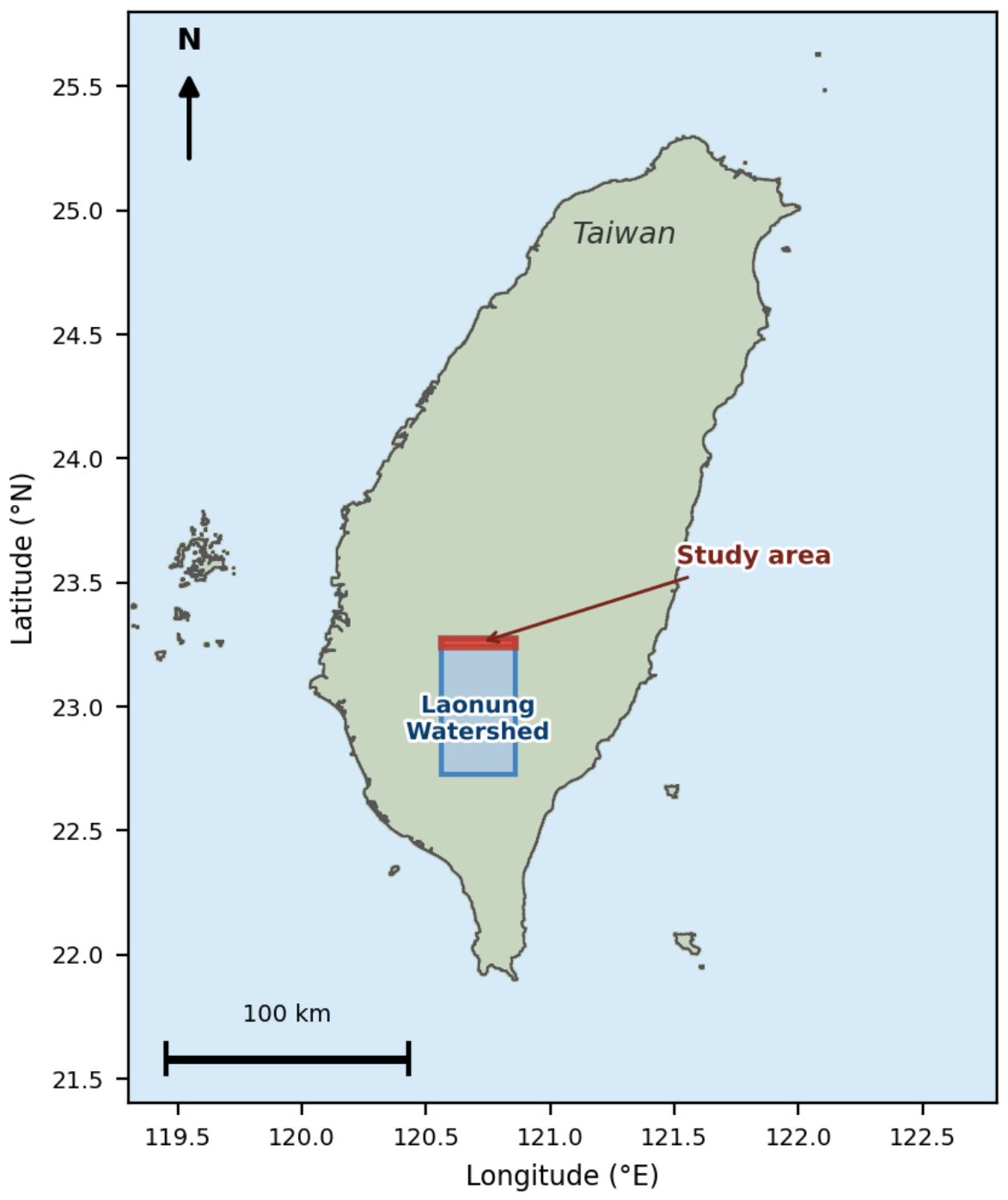
Figure 1 presents the overall spatial coverage of the study area, together with the position of the annotated pilot subregion within the complete tile grid. The pilot study area comprises the northernmost four rows of tiles (rows 1–4, columns 1–32), covering approximately 116 km². The spatial distribution of the annotated tiles and the cross-validation fold assignments used in the pilot analysis are shown in Figure 2.

3. Data and Methods

The following section details the data sources, labeling framework, and sequence of analyses implemented in this work. The overall pipeline is as follows: DEM tiles and co-registered SPOT-6 imagery tiles serve as the primary data inputs; geomorphometric and spectral features are extracted at the pixel level; landslide masks produced through expert-guided annotation in CVAT (Computer Vision Annotation Tool; https://www.cvat.ai/) provide the reference labels; and three machine learning classifiers are trained and evaluated under a spatially blocked cross-validation scheme designed to reduce leakage between geographically adjacent tiles. Feature interpretability is examined using SHAP analysis conducted across all four spatial folds of the selected tree-based model, with one held-out fold examined in detail as a representative case. The pipeline is designed to be methodologically transparent and transferable so that it can be reapplied consistently as annotation expands, providing the methodological continuity required for sustainable, long-term landslide monitoring of the watershed. Because this is a pilot study based on annotated tiles from a limited subregion and evaluated on a resampled pixel distribution, the reported performance should be interpreted within that experimental setting.

3.1. Data Sources and Tile Structure

Recent advances in airborne LiDAR and UAV-based surveying have made very high-resolution digital elevation models increasingly available for geomorphological and hazard-related studies, with spatial resolutions that may approach the sub-meter or even centimeter scale. In this study, the topographic dataset is a proprietary airborne LiDAR-derived DEM whose exact spatial resolution is not disclosed for confidentiality reasons. Nevertheless, the dataset belongs to the class of very high-resolution terrain data and is suitable for detailed pixel-level landslide analysis. The 2024 DEM was used as the primary dataset and was divided into 2048 tiles using a regular grid. Each tile measures $953\times 947$ pixels. Tiles are identified by a matrix index (r{row}_c{col}), with 32 tiles per row and 64 rows in total, numbered from the upper-left corner.

Multispectral imagery acquired by SPOT-6 was supplied through the Center for Space and Remote Sensing Research at National Central University, Taiwan. Two acquisition dates were used: 13 January 2025 as the primary source and 17 September 2024 as supplementary coverage where cloud contamination affected the primary acquisition. The September acquisition was therefore used only as cloud gap-fill on a minority of tiles rather than as a co-equal seasonal composite, so the dataset is not a balanced two-season sample. The SPOT-6 imagery was resampled and co-registered to the DEM grid using bilinear resampling, producing one four-band tile for each DEM tile. All raster datasets are referenced to the Taiwan Datum 1997 (TWD97) coordinate system and retain complete georeference metadata, including the coordinate reference system, geotransform, and spatial extent, thereby ensuring pixel-level alignment among all layers within each tile. The SPOT-6 sensor (Airbus Defence and Space, Toulouse, France) records four multispectral bands, including blue (450–525 nm), green (530–590 nm), red (625–695 nm), and near-infrared (760–890 nm). The data have a 12-bit radiometric resolution and are stored as 16-bit unsigned integers, corresponding to an effective digital number range of 0–4095. Because the DEM and SPOT-6 data were not acquired on identical dates, the mapped landslide condition should be interpreted with this temporal mismatch in mind.

3.2. Landslide Annotation Framework

Landslide annotations were produced manually in the Computer Vision Annotation Tool (CVAT) platform [53], while Segment Anything Model 3 (SAM 3; arXiv preprint) was used as an interactive aid for boundary delineation [54]. A total of 128 tiles were annotated, of which 96 contain at least one landslide polygon. Annotation targeted current landslides, defined operationally as areas showing optical evidence of recent bare-soil exposure or vegetation disturbance in the SPOT-6 imagery, rather than historical landslide terrain visible only in DEM morphology. This definition was adopted to promote more consistent interpretation across the annotated tiles, although the delineation of geomorphic units remains dependent on expert judgment.

The interpretation protocol followed a defined priority order. SPOT-6 optical imagery was consulted first to identify bare soil, fresh collapse tones, and vegetation discontinuities indicative of recent mass movement. DEM-derived hillshade was then used to verify geomorphic context and refine boundary placement. Final delineations followed geomorphic-unit boundaries, including the scarp, body, and accumulation zone, rather than spectral patch edges alone. This approach was intended to improve annotation consistency and to produce labels representing the interpreted physical extent of each landslide event. Ambiguous areas were cross-checked against orthophotos provided by the National Land Surveying and Mapping Center and Google Earth historical imagery. SAM 3 accelerated boundary fitting, but all interpretive decisions were made by the human annotator.

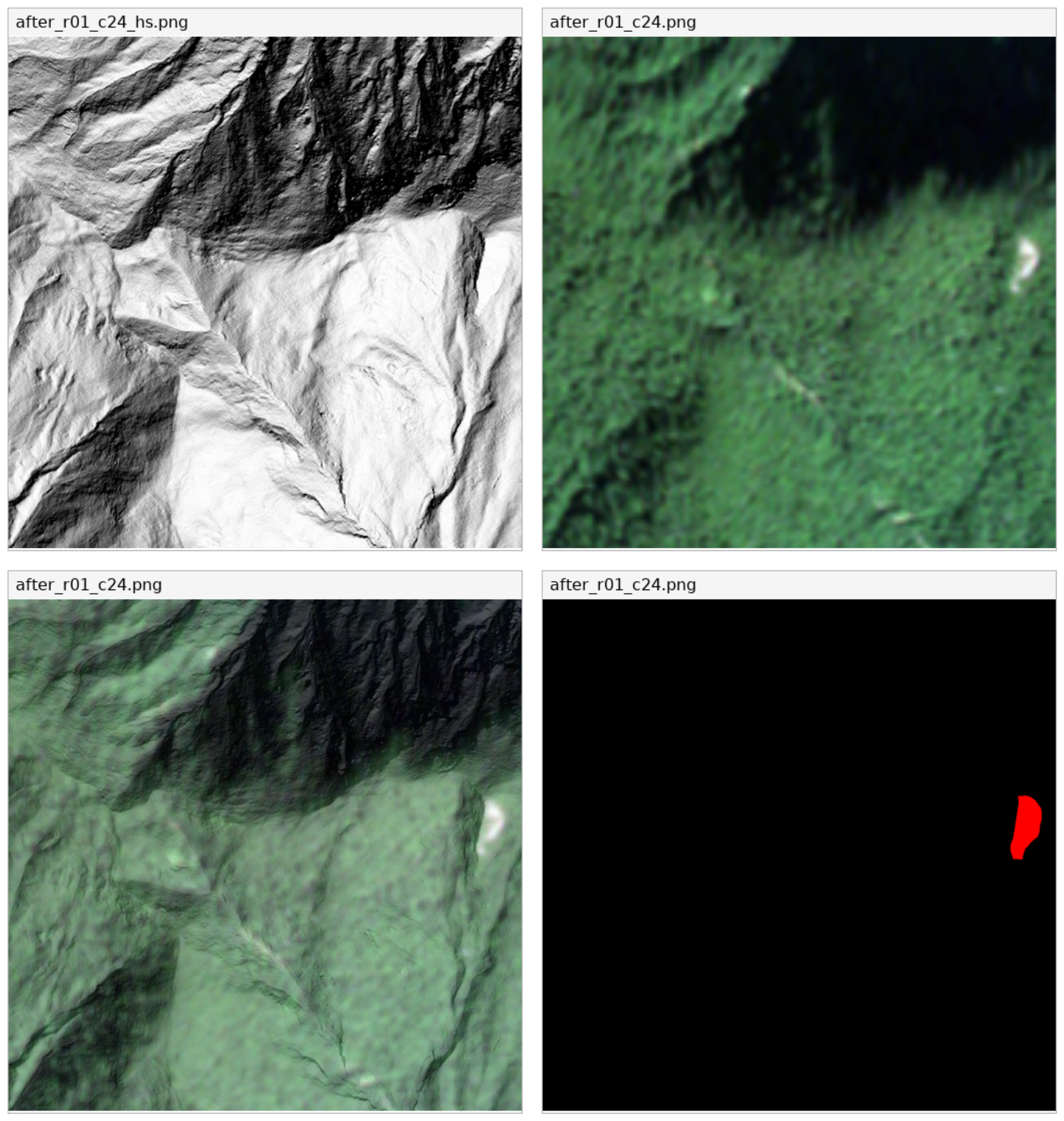
Figure 3 illustrates the annotation workflow for a representative tile (r01_c24). The top-left panel shows the hillshade, which highlights the topographic morphology of the interpreted landslide, including the scarp area and irregular slope surface. The top-right panel shows the SPOT-6 natural color composite, which provides the optical evidence used to identify recent bare-soil exposure. The bottom-left panel shows the fused composite, which served as the annotation input in CVAT by combining both sources of evidence into a single three-band image. The bottom-right panel shows the resulting expert delineation mask. In this example, the delineation follows the interpreted geomorphic-unit extent rather than the spectral patch edge alone and includes areas where terrain morphology suggests landslide extent beyond the optically brightest bare-soil surface.

To support CVAT ingestion, DEM-derived hillshade (PNG format) and SPOT-6 RGB imagery were fused into a three-band composite used exclusively as a visual annotation aid. Hillshade served as the base layer, whereas SPOT-6 RGB was contrast-enhanced using a per-band 2nd–98th percentile linear stretch to 8-bit and composited over the hillshade at 70% opacity. This fused composite was used only to support visual interpretation during annotation and was not used as a model input.

3.3. Feature Extraction

Thirteen features were extracted per pixel from georeferenced GeoTIFF layers (

Table 1. Feature set used for pixel-level landslide classification. B1–B4 refer to the SPOT-6 Blue, Green, Red, and Near-Infrared (NIR) bands, respectively.

Feature	Category	Definition
DEM	Topographic	Digital Elevation Model; elevation (m)
Slope	Topographic	Local slope angle (degrees)
Curvature	Topographic	Profile curvature: the second derivative of the elevation surface in the direction of maximum slope, quantifying the rate of change in slope angle along the steepest descent direction
SPOT B1	Spectral	Blue band (450–525 nm), UInt16
SPOT B2	Spectral	Green band (530–590 nm), UInt16
SPOT B3	Spectral	Red band (625–695 nm), UInt16
SPOT B4	Spectral	Near-Infrared band (760–890 nm), UInt16
NDVI	Index	Normalized Difference Vegetation Index, $(B4-B3)/(B4+B3)$
SAVI	Index	Soil-Adjusted Vegetation Index, $\left[\right(B4-B3)/(B4+B3+0.5\left)\right]\times 1.5$
EVI	Index	Enhanced Vegetation Index, $2.5\times (B4-B3)/(B4+6B3-7.5B1+1)$
BI	Index	Brightness Index, $\sqrt{(B{3}^2+B{4}^2)/2}$; this red–NIR formulation was used as a simple spectral brightness measure and may differ from other BI definitions in the literature
BSI	Index	Bare Soil Index, $\left[\right(B3+B1)-(B4+B2\left)\right]/\left[\right(B3+B1)+(B4+B2\left)\right]$; this is a SPOT-6-adapted visible–near-infrared formulation because SPOT-6 does not provide a shortwave-infrared band
NDWI	Index	Normalized Difference Water Index, $(B2-B4)/(B2+B4)$; this corresponds to the green–NIR formulation of NDWI

). The topographic features were DEM elevation, slope (degrees), and profile curvature, all derived from the 2024 DEM. The spectral features were the four raw SPOT-6 bands stored as UInt16 values (0–4095). Six spectral indices were computed from the raw band values using float32 precision to avoid integer overflow (Table 1). Two of these indices use formulations adapted to the four-band SPOT-6 sensor, which acquires only visible and near-infrared bands. The standard Bare Soil Index, $\left[\right(\mathrm{SWIR}+\mathrm{Red})-(\mathrm{NIR}+\mathrm{Blue}\left)\right]/\left[\right(\mathrm{SWIR}+\mathrm{Red})+(\mathrm{NIR}+\mathrm{Blue}\left)\right]$, requires a shortwave-infrared band and therefore cannot be computed from SPOT-6 imagery; a four-band adaptation of the same normalized-difference form was used instead, with the red and blue bands in the positive term and the near-infrared and green bands in the negative term, preserving the normalized soil-minus-vegetation contrast structure of the index while using only the available SPOT-6 bands. The Brightness Index was computed as the root-mean-square of the red and near-infrared bands. Brightness indices are not standardized to a single definition in the literature and are commonly formed from the root-mean-square of two or more reflectance bands; the red and near-infrared bands were used here because fresh landslide surfaces are bright in both, providing a simple magnitude measure of overall surface reflectance suited to separating exposed soil and rock from vegetated terrain. Both formulations may therefore differ from indices of the same name used with sensors that include a shortwave-infrared band or a different band selection. Pixels that produced undefined index values because of zero denominators were recorded as NaN and were handled by median imputation during preprocessing. The hillshade and fused composite layers were excluded from model input because they were generated for visual interpretation only and were not used as analytical raster inputs.

3.4. Pixel Sampling Strategy

Pixel-level classification required sampling from the full raster stack. To manage the computational scale while preserving representation of the positive class, all landslide pixels were retained from each annotated tile, and background pixels were randomly sampled at a 3:1 ratio relative to landslide pixels within each tile (random seed 42). This procedure produced a dataset of 5,809,508 pixels (1,452,377 positive; 4,357,131 negative), corresponding to a 3:1 negative-to-positive class ratio and a sampled positive prevalence of 25.0%. For context, the natural positive pixel prevalence across the 128 annotated tiles is approximately 1.7% (mean landslide fraction per tile). However, because model training and evaluation were both conducted on the resampled pixel distribution, the reported performance metrics should be interpreted with respect to that sampled distribution rather than as direct estimates under the natural class prevalence of the broader study area.

3.5. Spatial Cross-Validation Design

A four-fold spatially blocked cross-validation strategy was adopted to reduce spatial leakage between training and test sets. The 96 annotated tiles containing landslides occupy rows 1–4 of the tile grid and span all 32 columns. Folds were defined by column quartiles: Fold 1 (columns 1–8), Fold 2 (columns 9–16), Fold 3 (columns 17–24), and Fold 4 (columns 25–32). Each fold therefore represents a geographically contiguous subregion, ensuring that no tile contributes pixels to both the training and test datasets in any iteration. The spatial distribution of the annotated tiles and their fold assignments is shown in Figure 2. Fold sizes ranged from 20 to 29 tiles, reflecting the uneven spatial distribution of the annotated landslide-containing tiles across columns (

Table 2. Spatial cross-validation fold composition. LS = landslide.

Fold	Columns	Tiles	Mean LS Fraction	Pixels (Sampled)
1	1–8	23	0.014	1,140,448
2	9–16	24	0.014	1,254,980
3	17–24	20	0.011	760,212
4	25–32	29	0.025	2,653,868
Total	1–32	96	0.017	5,809,508

). This design was intended to provide a more conservative assessment than random splitting, although the results remain conditional on the annotated pilot subregion and the resampled pixel distribution used in this study.

3.6. Preprocessing

Within each cross-validation fold, all preprocessing steps were fitted exclusively on the training set and then applied to the test set to reduce data leakage. SPOT-6 band values were normalized to [0, 1] by dividing by 4095. NaN values arising from undefined spectral-index computations (0.051% of EVI values and zero for all other indices) were replaced with the training-set median of the corresponding feature. All predictor variables were subsequently standardized by applying a standard scaler fitted only to the training fold, thereby transforming each feature to have a mean of zero and a standard deviation of one.

3.7. Classification Models

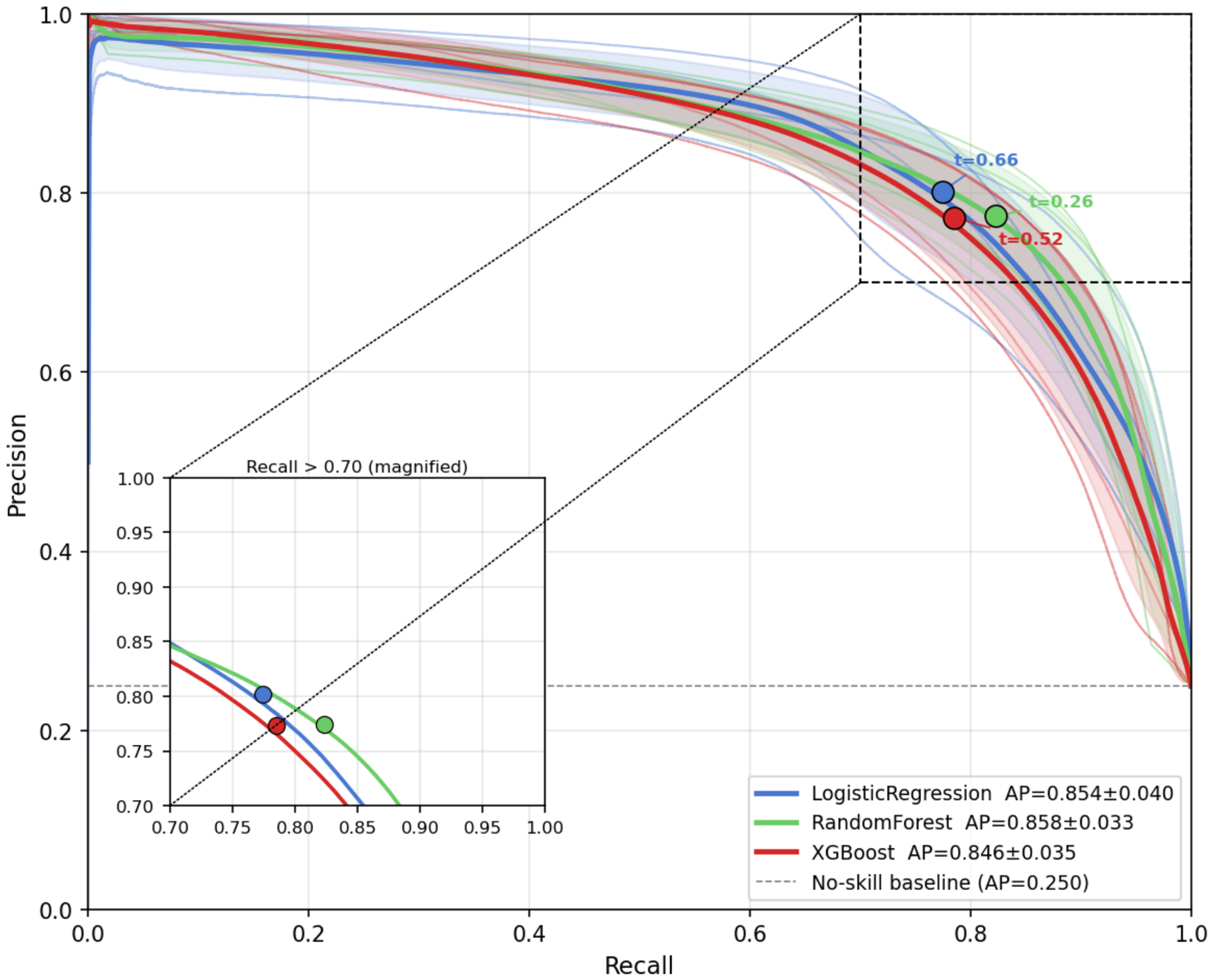
Three classifiers were selected to span a range of model complexity, from linear to nonlinear ensemble methods, allowing the study to assess whether the landslide classification signal in the present feature set is linearly separable or whether nonlinear modeling is needed. Logistic regression (LR) is a linear probabilistic classifier that estimates the probability of class membership as a sigmoid function of a weighted linear combination of input features; it serves as an interpretable linear baseline. Random forest (RF) is an ensemble of decision trees trained on bootstrap samples of the data, with each tree using a random subset of features at each split; by averaging predictions across many decorrelated trees, RF reduces variance relative to a single decision tree and is robust to class imbalance when balanced class weights are applied. XGBoost is a gradient-boosted ensemble method that builds trees sequentially, with each tree correcting the residual errors of the previous ensemble; it is widely used in geospatial machine learning due to its computational efficiency and strong predictive performance across diverse feature sets. The models were implemented as follows. Logistic regression (LR) was used as a linear reference model, with class imbalance addressed by applying balanced class weights (class_weight=‘balanced’). Random forest (RF) was trained with 300 estimators and balanced class weights. XGBoost was trained with 300 estimators and a positive class weight of 3.0, reflecting the 3:1 negative-to-positive sampling ratio. The remaining hyperparameters, including the learning rate (eta = 0.3) and maximum tree depth (max_depth = 6), were left at their library defaults. Hyperparameters were specified a priori and were not tuned on the test data; the default learning rate of 0.3 is a relatively aggressive setting, and we did not perform a sensitivity sweep over it in this pilot (see Section 5.4). All random states were fixed at 42. All models were evaluated at the default classification threshold of 0.5, whereby a pixel was assigned to the landslide class if its predicted probability met or exceeded this value; for Random Forest, whose vote-based probabilities can equal 0.5 exactly, ties were assigned to the landslide class, consistent with this threshold rule. This threshold was not optimized and should be interpreted as a fixed reference threshold for comparison across models rather than as an application-specific optimum. Alternative thresholds can be selected from the precision–recall curves (Figure 4) to adjust the precision–recall trade-off according to application requirements; however, such threshold choices should be interpreted separately from the primary evaluation at the default threshold.

3.8. Evaluation Metrics

Model performance was evaluated using precision, recall, F1 score, the area under the receiver operating characteristic curve (ROC-AUC), and average precision (AP), which corresponds to the area under the precision–recall curve. Average precision is emphasized as the primary metric because of the class imbalance in the sampled dataset. The no-skill baseline for the sampled dataset is AP $=0.250$, corresponding to the 25% positive-class prevalence after resampling; this is the appropriate reference for comparing model AP values within the present experimental design because all models were trained and evaluated on the same resampled distribution. ROC-AUC is reported as a secondary summary metric. For each metric, values were first calculated separately for each fold and then reported as the mean ± standard deviation across the four spatial folds.

Per-tile error metrics reported in Section 4.4 were computed from the same 3:1 sampled pixel subset used for model training and evaluation, ensuring consistency with the fold-level metrics. Fold-level recall values were computed as pixel-weighted averages across all sampled pixels in each test fold, whereas per-tile false negative rates were computed independently for each tile. These per-tile values are therefore not directly comparable to fold-level recall because of differences in tile size and landslide pixel count. More broadly, all reported metrics should be interpreted within the sampled evaluation setting used in this pilot study rather than as direct estimates under the natural class prevalence of the full watershed. The metrics reported here differ in how they respond to this prevalence choice. Recall, the false-negative rate, and ROC-AUC are based on class-conditional quantities. Recall and FNR are computed only over the positive landslide class, while ROC-AUC summarizes the ranking of positive and negative samples through true-positive and false-positive rates. These quantities are therefore largely invariant to positive prevalence, provided that the sampled positives and negatives are representative of their natural class-conditional distributions. However, ROC-based assessment should still be interpreted cautiously in this rare-event setting, because a seemingly small false-positive rate may correspond to many false-positive pixels when the negative class dominates the landscape.

Precision, the precision–recall curve, and average precision are more directly affected by prevalence. At the natural landslide prevalence of approximately 1.7%, the negative-to-positive ratio is about 57.8:1, compared with 3:1 in the resampled 25% positive setting. Thus, for the same recall and false-positive rate, the false positives contributing to precision would arise from a negative pool roughly nineteen times larger per positive case than in the resampled evaluation. Precision at any fixed recall would therefore be substantially lower, except in the limiting case of nearly zero false positives. Similarly, the no-skill AP baseline would fall from 0.250 in the resampled evaluation to approximately 0.017 under the natural prevalence. The AP and PR-curve results reported here should accordingly be read as characterizing the resampled evaluation distribution. Operationally realistic precision and AP at natural prevalence are best quantified through full-tile evaluation at the true class balance, as pursued in the companion study [49] and identified as future work for the full watershed.

3.9. SHAP Computation and Analysis Procedure

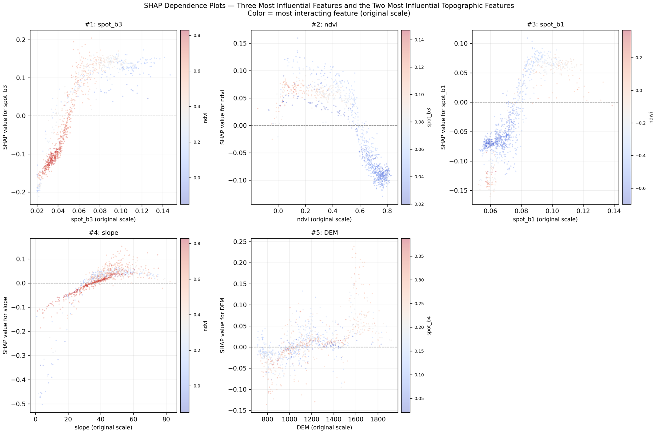
SHapley Additive exPlanations [50] were computed for the selected tree-based model (Random Forest) using the shap Python library with TreeExplainer. Two complementary SHAP analyses were conducted. First, to assess the stability of feature contributions across spatial blocks, SHAP values were computed for all four spatial folds: for each fold, the Random Forest model was retrained on the other three folds and evaluated on a stratified sample of 2000 pixels (1000 positive and 1000 negative; random seed 42) from the held-out fold, yielding 8000 explained pixels in total. This cross-fold analysis provides the mean absolute SHAP value rankings and their across-fold variability. Second, for detailed directional and interaction analysis, the model trained on folds 1–3 combined was examined on the held-out fold 4, which contains the largest number of tiles and the highest mean landslide fraction, using a stratified subsample of 1000 pixels from the fold 4 test set (500 positive, 500 negative; random seed 42). This fold-4 sample provides the beeswarm summary plot and the dependence plots for the three most influential features overall and the two most influential topographic features, presented as a representative case of model behavior within the present study design.

3.10. Software Environment

All analyses were implemented in Python 3.11.11 within a dedicated conda environment. The main libraries used were scikit-learn 1.8.0 for logistic regression, random forest, preprocessing, and evaluation metrics [55]; XGBoost 3.2.0 for the gradient-boosted classifier [56]; shap 0.51.0 with TreeExplainer for SHAP interpretability analysis [50]; rasterio 1.4.4 for geospatial raster input and output; numpy 2.4.3 for array operations; and matplotlib 3.10.8 for figure generation. Landslide annotation was performed in CVAT [53] with SAM 3 assistance [54]. The conda environment specification is available from the corresponding author upon reasonable request.

4. Results

The results are presented in six subsections. Section 4.1 reports classification performance across the three models and four spatial folds, with average precision as the primary metric. Section 4.2 presents feature-importance rankings derived from the tree-based models. Section 4.3 presents the SHAP interpretability analysis for Random Forest. Section 4.4 examines the spatial distribution of classification errors across the tile grid. Section 4.5 reports the results of threshold optimization as a secondary sensitivity analysis of the precision–recall trade-off. Section 4.6 assesses the probability calibration of the Random Forest model on the resampled evaluation distribution.

4.1. Classification Performance

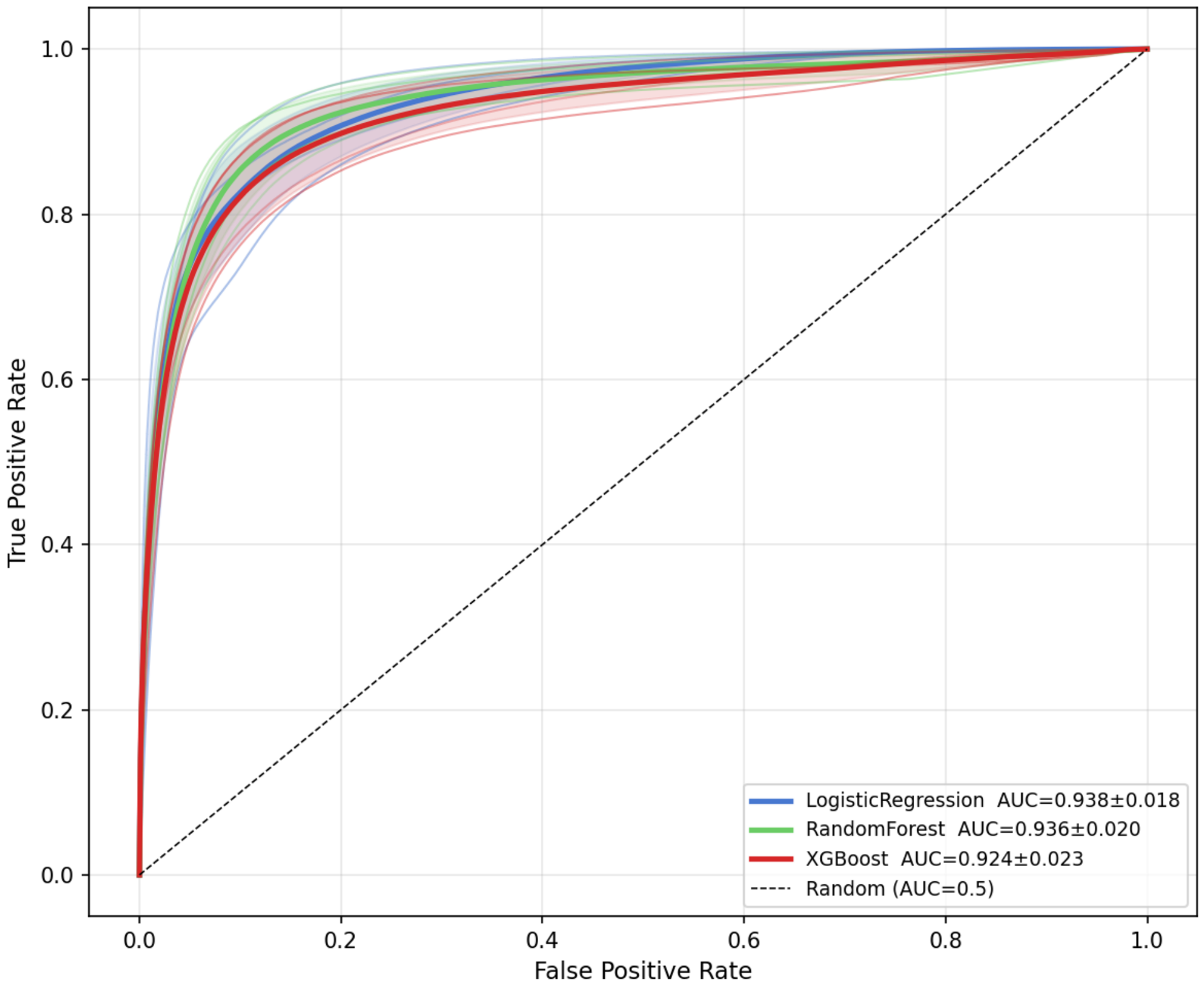
All three classifiers substantially outperformed the no-skill baseline for the resampled evaluation dataset (AP $=0.250$) across all four spatial folds (

Table 3. Cross-validated classification performance (mean ± standard deviation across four spatial folds). AP = average precision. All metrics were computed on the resampled evaluation dataset.

Model	Precision	Recall	F1	ROC-AUC	AP
Logistic Regression	$0.732\pm 0.087$	$0.830\pm 0.079$	$0.772\pm 0.038$	$0.938\pm 0.021$	$0.854\pm 0.040$
Random Forest	$0.858\pm 0.033$	$0.681\pm 0.095$	$0.755\pm 0.062$	$0.936\pm 0.023$	$0.858\pm 0.033$
XGBoost	$0.762\pm 0.056$	$0.792\pm 0.055$	$0.775\pm 0.037$	$0.924\pm 0.026$	$0.846\pm 0.035$

; Figure 4). Mean AP values were $0.854\pm 0.040$ for LR, $0.858\pm 0.033$ for RF, and $0.846\pm 0.035$ for XGBoost. These values correspond to AP values approximately 3.4 times the no-skill baseline within the sampled evaluation setting. ROC-AUC values (Figure 5) were also high across all models (0.924–0.938), although AP is emphasized as the primary metric because of class imbalance and because all models were evaluated on the same resampled class distribution.

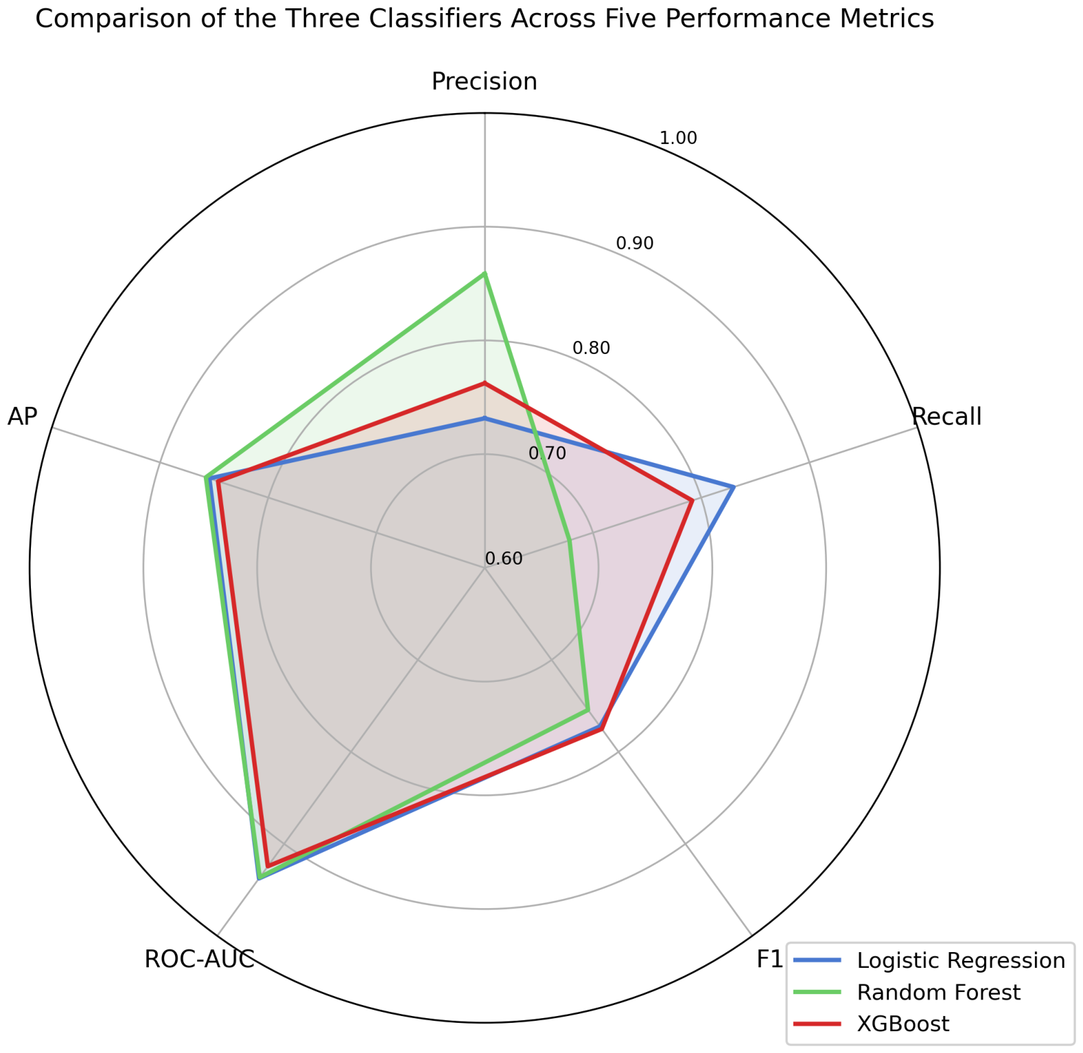
The three models showed similar overall precision–recall performance, with only modest differences among them (Table 3; Figure 4). Random Forest achieved the highest mean average precision (AP $=0.858\pm 0.033$), followed closely by Logistic Regression (AP $=0.854\pm 0.040$), whereas XGBoost showed a slightly lower mean AP ($0.846\pm 0.035$). At the default classification threshold of 0.5, however, the models occupied different points along the precision–recall trade-off. Random Forest achieved the highest precision ($0.858\pm 0.033$) but the lowest recall ($0.681\pm 0.095$), indicating that, under this fixed threshold, it produced fewer false positives at the cost of more missed landslide pixels. Logistic Regression showed the highest recall ($0.830\pm 0.079$) with lower precision ($0.732\pm 0.087$), indicating a less conservative prediction profile at the same threshold. XGBoost achieved the highest F1 score ($0.775\pm 0.037$), with intermediate precision ($0.762\pm 0.056$) and recall ($0.792\pm 0.055$), indicating the most balanced performance among the three models at the default threshold. Figure 6 summarizes these comparisons across all five metrics, showing the complementary strengths of the three models: random forest in precision, logistic regression in recall, and XGBoost in balance, with convergence at high ROC-AUC and AP. To assess whether the small differences in mean AP among the three models are statistically distinguishable, we computed the pairwise AP differences and estimated 95% confidence intervals using a stratified tile-level bootstrap (1000 iterations, seed 42), resampling tiles within each spatial fold and paired across models, and applying the same mean-of-per-fold AP estimator used throughout. The Logistic Regression–Random Forest difference ($-0.003$; 95% CI $[-0.014,+0.010]$) and the Logistic Regression–XGBoost difference ($+0.008$; 95% CI $[-0.004,+0.024]$) both have confidence intervals that include zero, indicating that these pairs are not statistically distinguishable in average precision. The Random Forest–XGBoost difference ($+0.011$; 95% CI $[+0.004,+0.021]$) excludes zero, indicating a small but statistically detectable advantage for Random Forest over XGBoost, which exceeded XGBoost in three of the four folds. This margin of approximately $0.011$ AP is negligible in practical terms, and the two comparisons involving the linear baseline remain statistically indistinguishable; the formal test therefore reinforces, rather than qualifies, the observation that models of differing complexity achieve closely comparable average precision on this feature set. Threshold-optimization results are reported separately in Section 4.5 as a secondary sensitivity analysis.

To assess whether the machine learning framework is necessary given the dominance of SPOT-6 Band 3 and NDVI (Section 4.2), we evaluated a simpler baseline: a logistic regression using only these two features, under the identical spatially blocked cross-validation and preprocessing. This two-feature baseline achieved a mean AP of $0.805\pm 0.087$, recovering approximately 92% of the skill of the full 13-feature logistic regression (AP $0.854\pm 0.040$) above the no-skill baseline of 0.250, and falling short of the best full-feature model (Random Forest, AP $0.858$) by 0.053. A single-feature model using Band 3 alone reached a comparable AP ($0.811\pm 0.089$), whereas NDVI alone was substantially weaker ($0.524\pm 0.117$); adding NDVI to Band 3 did not increase AP, although it improved ROC-AUC (from 0.903 to 0.924) and precision. This confirms that the dominant discriminatory signal is concentrated in a small number of spectral features, consistent with the feature-importance and SHAP analyses, and that much of the classification performance is recoverable from Band 3 alone. The full feature set and the machine learning framework nonetheless provide the incremental performance above this baseline, the interpretability afforded by SHAP attribution, the per-tile spatial error characterization reported below, and additional headroom should the dominant spectral cues degrade under other imaging or seasonal conditions.

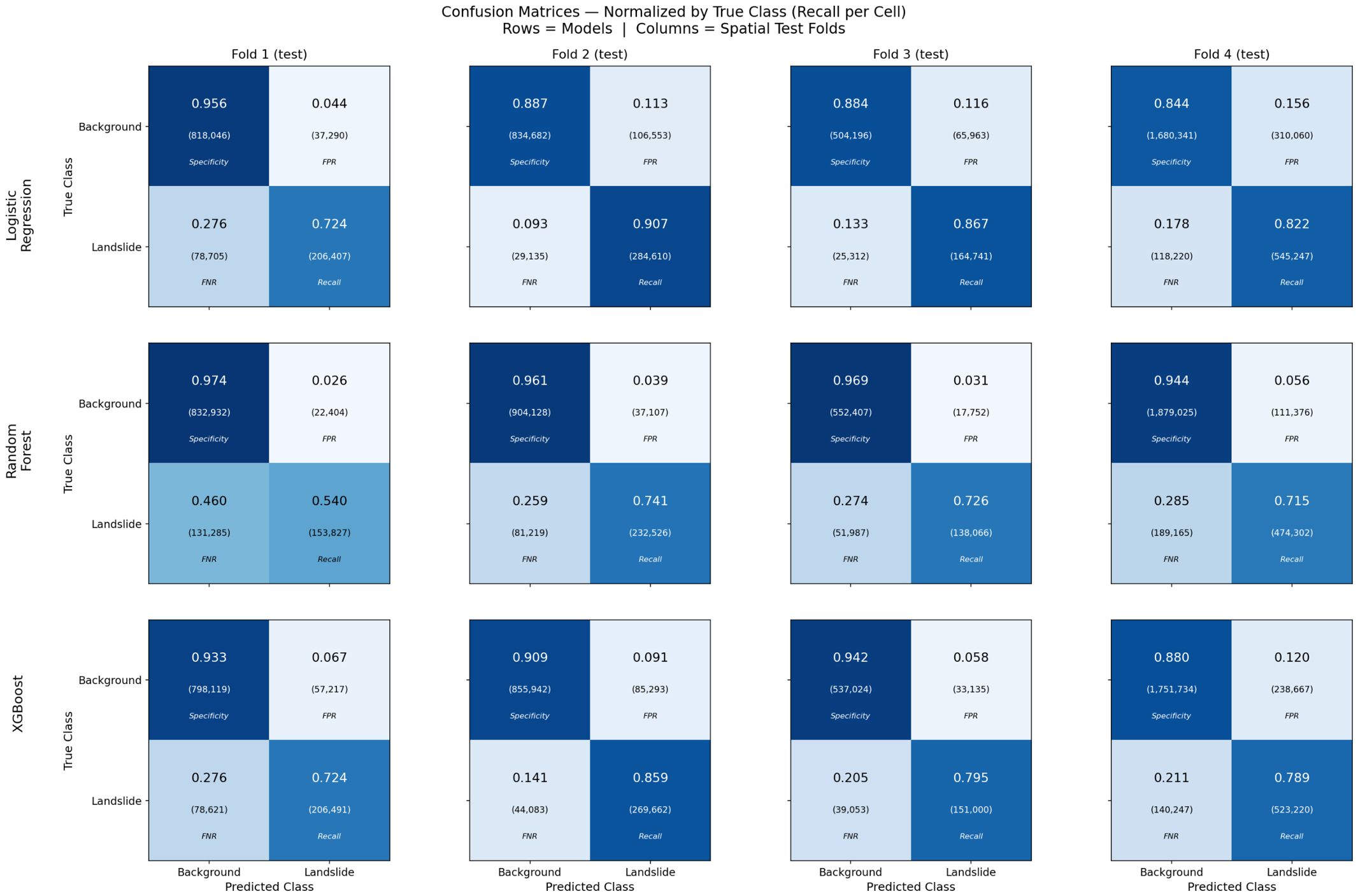
Per-fold performance varied moderately across spatial blocks (Figure 7). In the row-normalized confusion matrices (Figure 7), the upper-left cell represents the fraction of background pixels correctly classified as background (specificity), and the lower-right cell represents the fraction of landslide pixels correctly classified as landslide (recall), whereas the off-diagonal cells represent the false positive rate (upper right) and false negative rate (lower left), respectively. For RF, Fold 1 produced notably lower landslide recall (0.540) than Folds 2–4 (0.715–0.741), indicating that this spatial block was more difficult for that model under the present study design. For LR and XGBoost, Fold 4 produced the lowest F1 scores despite containing the highest mean landslide fraction (0.025). This pattern may reflect differences in landslide size, morphology, vegetation cover, or other spatially varying characteristics within columns 25–32, although these possible explanations were not directly tested in the present study.

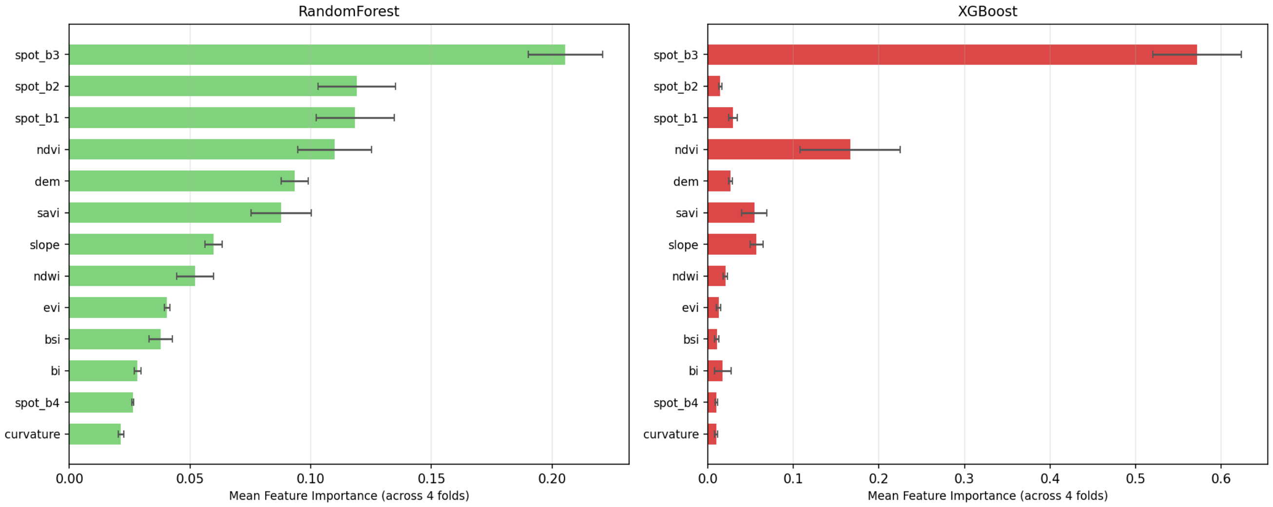
4.2. Feature Importance

Random Forest and XGBoost feature-importance rankings showed partial agreement on the dominant predictors, with substantial differences in how importance was distributed across features (Figure 8). In both models, SPOT-6 Band 3 (Red) was the most important feature, accounting for approximately 21% of RF importance and 57% of XGBoost importance. In Random Forest, importance was distributed more broadly across several spectral and topographic variables, with SPOT-6 Bands 1–3, NDVI, DEM elevation, SAVI, and slope all contributing non-negligibly. In XGBoost, by contrast, importance was concentrated much more heavily on Band 3, with NDVI as the only clearly secondary predictor and the remaining features contributing relatively little. This pattern is consistent with the prominence of spectral information related to bare-soil exposure and vegetation condition in the present pilot dataset, although the strong importance of these variables should also be interpreted in light of the annotation protocol, which used optical evidence as the primary basis for identifying current landslide activity. Curvature was the weakest predictor in both models, which may reflect high local variability at very high-resolution and limited per-pixel discriminative value under the current feature set. It should be noted that Random Forest importance values reflect the mean decrease in Gini impurity, whereas XGBoost importance values reflect normalized gain across all splits; these measures are computed using different mechanisms and are not directly numerically comparable across the two models. The contrast in how importance is distributed is itself partly attributable to these mechanisms: mean decrease in Gini impurity, averaged over many decorrelated trees, tends to spread importance across correlated spectral predictors, whereas boosted-tree gain tends to accrue to whichever single feature a split exploits first, concentrating importance on a dominant cue such as Band 3. Notably, this difference in importance distribution is not accompanied by a corresponding difference in predictive performance, as the two models achieved similar average precision (0.846 for XGBoost versus 0.858 for Random Forest). The concentration in XGBoost therefore cannot be attributed to overfitting, nor the broader Random Forest distribution to superior generalization, on the basis of the importance patterns alone. Overall, the two models appear to have used the available feature set in different ways within the present pilot dataset, but the feature-importance results alone do not establish that one model is necessarily more robust than the other under changing imaging or environmental conditions. To characterize the multicollinearity structure underlying these importance patterns, variance inflation factors (VIFs) were computed for the 13-feature set on a random subsample of 100,000 pixels (

Table 4. Variance inflation factors (VIFs) for the 13-feature set, computed on a random subsample of 100,000 pixels with an intercept term included. Values are sorted in descending order. High VIFs among the spectral features reflect their construction from a shared set of four SPOT-6 bands.

Feature	VIF
SAVI	>${10}^4$
NDVI	>${10}^4$
BI	5049.3
SPOT B4	4917.0
BSI	1155.5
NDWI	359.3
SPOT B3	345.4
SPOT B2	331.7
SPOT B1	122.4
DEM	1.8
slope	1.1
EVI	1.0
curvature	1.0

). Nine of the thirteen features exceeded the conventional VIF threshold of 10, confirming substantial multicollinearity. This collinearity is concentrated in the spectral block: the vegetation indices and raw bands are deterministic functions of the same four SPOT-6 bands, and NDVI and SAVI in particular are near-collinear (their VIFs are numerically unstable, exceeding ${10}^4$), because SAVI reduces to an approximately linear rescaling of NDVI over the value range observed here. In contrast, the topographic features were effectively independent of the remainder of the feature set (DEM VIF $=1.8$; slope $=1.1$; curvature $=1.0$), as they cannot be reconstructed from the spectral predictors. EVI also had a low VIF ($1.0$) despite being a spectral index, because VIF measures only linear dependence and the blue-band term and nonlinear form of EVI make it not linearly reconstructable from the other features. The effective dimensionality of the feature set is therefore appreciably lower than 13. This collinearity structure directly explains the contrast between the two models’ importance distributions described above: because correlated predictors are substitutable, the mean-decrease-in-impurity mechanism of Random Forest spreads importance across the intercorrelated spectral features, whereas the gain mechanism of XGBoost concentrates it on a single representative of the correlated group (Band 3). Tree-ensemble classifiers are generally robust to multicollinearity for prediction, which affects the distribution of importance across correlated features rather than predictive accuracy; this is consistent with the similar average precision achieved by the two models despite their differing importance profiles.

4.3. SHAP Interpretability Analysis

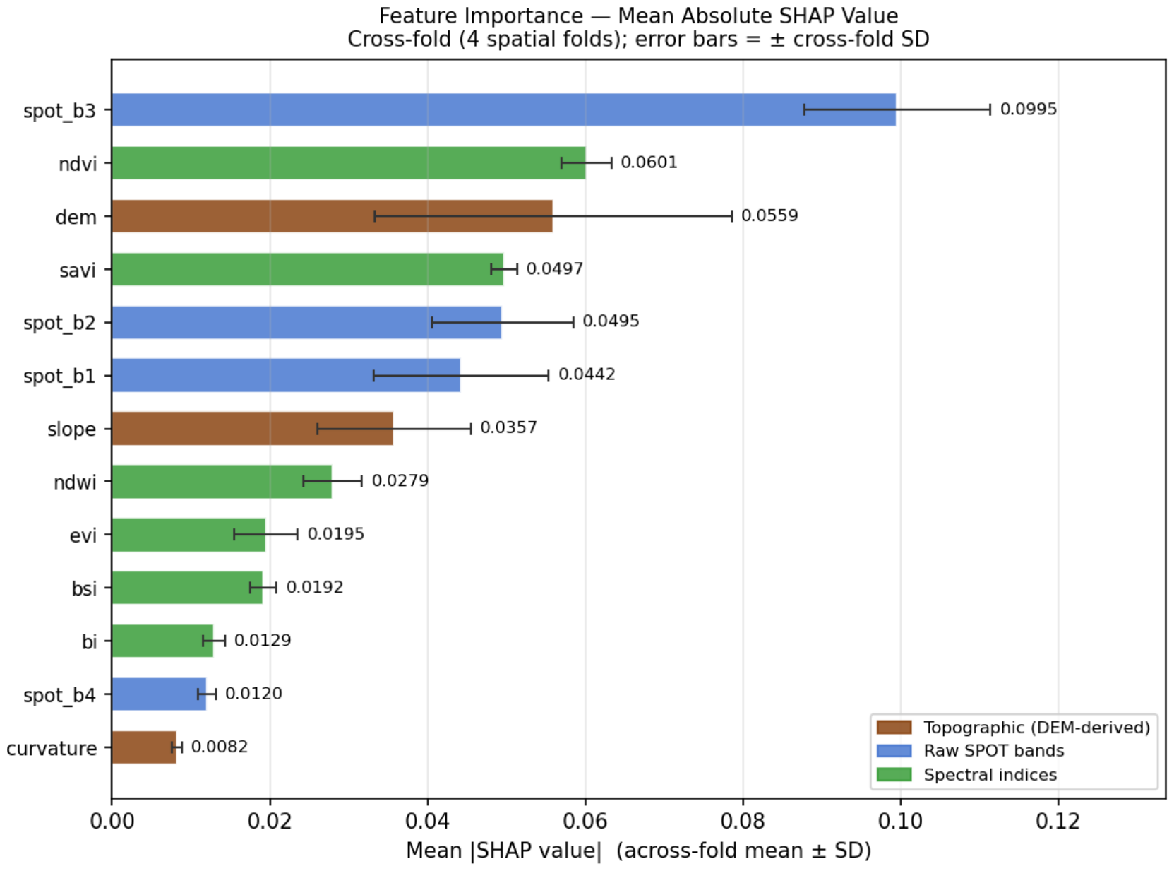
SHAP analysis was conducted across all four spatial folds: for each fold, the Random Forest model was retrained on the other three folds and mean absolute SHAP values were computed on a stratified sample of 2000 pixels (1000 positive and 1000 negative) from the held-out fold. The across-fold mean absolute SHAP values are shown in Figure 9, with error bars indicating ± one across-fold standard deviation. SPOT-6 Band 3 (Red) was the most influential feature in every fold (across-fold mean |SHAP|$=0.0995$), followed by NDVI ($0.0601$), with DEM elevation, SAVI, SPOT-6 Band 2 (Green), and SPOT-6 Band 1 (Blue) forming a group of secondary predictors of comparable magnitude. The importance structure was highly consistent across folds (pairwise Spearman rank correlations of $0.86$–$0.96$): Band 3 ranked first in all four folds, and NDVI was a stable secondary predictor, ranking in the top three in every fold and showing the smallest across-fold variability of the leading features. In contrast, the specific second-ranked feature varied by spatial block, and DEM elevation in particular ranged from second to seventh across folds, so its comparatively high across-fold mean should be read in light of this variability. Overall, the SHAP ranking is consistent with the strong role of spectral information in the present pilot dataset, while also indicating that topographic variables contributed additional information within the Random Forest model. The following analyses (Figure 10 and Figure 11) examine the held-out fold 4 in detail as a representative case (1000-pixel sample; Section 3.9); in that fold, the leading features were SPOT-6 Band 3 (mean |SHAP|$=0.105$), NDVI ($0.066$), SPOT-6 Band 1 ($0.063$), SPOT-6 Band 2 ($0.061$), and SAVI ($0.054$), with slope ($0.045$) and DEM elevation ($0.032$) contributing below the leading spectral variables.

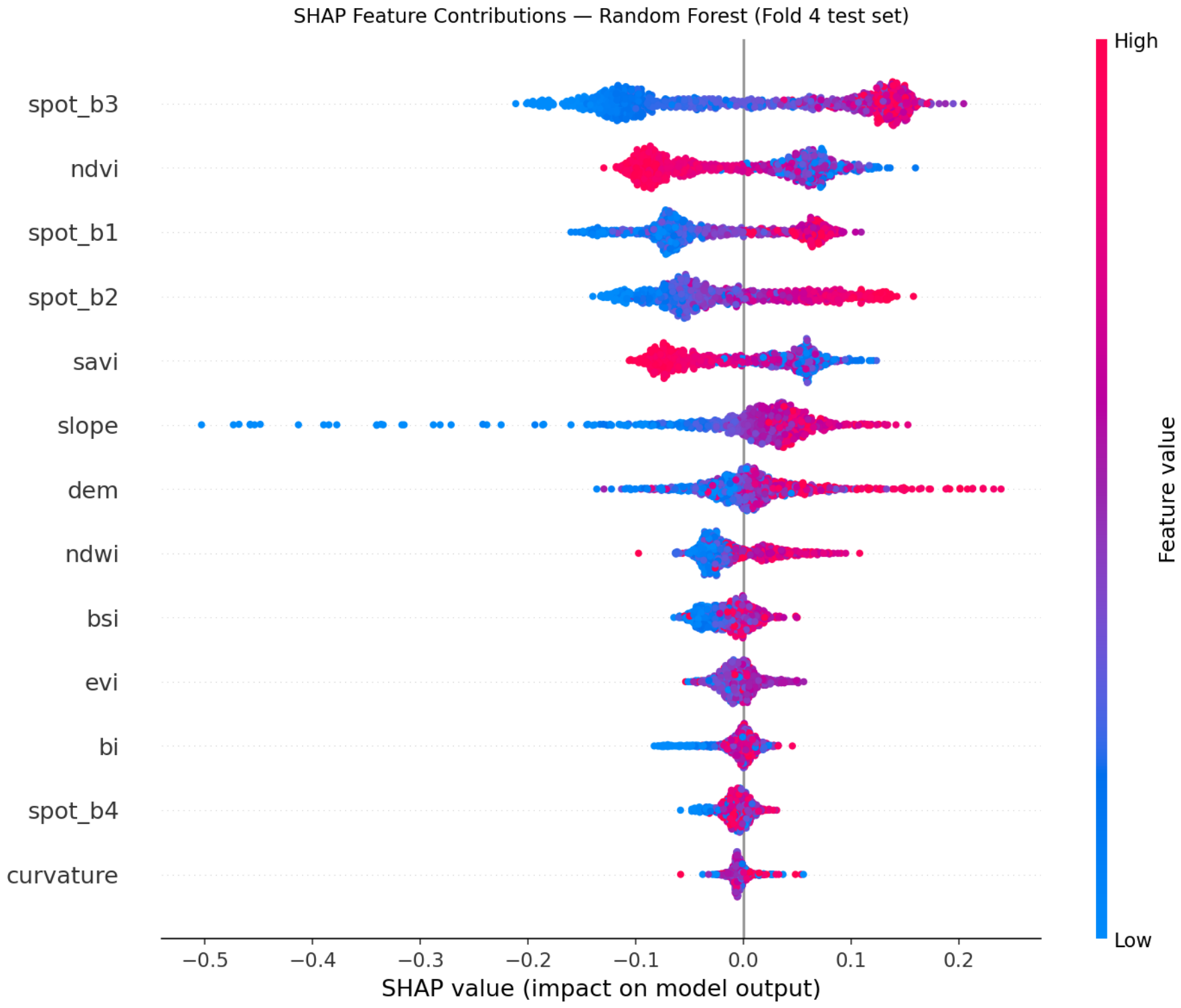
The beeswarm plot (Figure 10) shows the directional pattern of these feature contributions within the fold 4 SHAP sample. Higher SPOT-6 Band 3 values are generally associated with positive SHAP values, indicating increased predicted landslide probability, whereas higher NDVI values are generally associated with negative SHAP values. SAVI shows a similar overall tendency to NDVI. Slope also shows a tendency for higher values to contribute positively to landslide prediction. These patterns are consistent with the prominence of bare-soil spectral signals, reduced vegetation cover, and steeper terrain in the present pilot dataset, although they should be interpreted in the context of both the annotation protocol and the fold-specific SHAP analysis.

SHAP dependence plots for the three features with the greatest influence (Figure 11) show additional structure in the fold 4 SHAP sample. For SPOT-6 Band 3, higher values are generally associated with more positive SHAP values, with NDVI appearing as the strongest interaction variable: pixels with high red reflectance and low NDVI tend to receive the strongest positive SHAP contributions. For NDVI, the dependence plot shows an overall negative relationship, with lower NDVI values tending to be associated with more positive contributions to landslide prediction, particularly where Band 3 reflectance is high. For SPOT-6 Band 1 (Blue), the dependence plot indicates interaction with NDWI, suggesting that the contribution of blue reflectance to model output was influenced by related spectral variation in the present dataset. Extending the dependence analysis to the two most influential topographic features, slope and DEM elevation, shows that both contribute positively to predicted landslide probability. Higher slope values and higher elevations are generally associated with more positive SHAP values, with slope interacting most strongly with NDVI and DEM elevation interacting most strongly with SPOT-6 Band 4.

4.4. Spatial Distribution of Errors

Per-tile error analysis was conducted for the Random Forest model using the same 3:1 sampled pixel subset used for model training and evaluation, ensuring consistency with the fold-level metrics reported in Section 4.1. Pixel-weighted fold-level false negative rates (FNR $=1-$ recall) computed from saved predictions matched the corresponding recall-derived values across all four folds. The pixel-weighted mean FNR across folds was 0.319, corresponding to the mean Random Forest recall of 0.681 reported in Table 3.

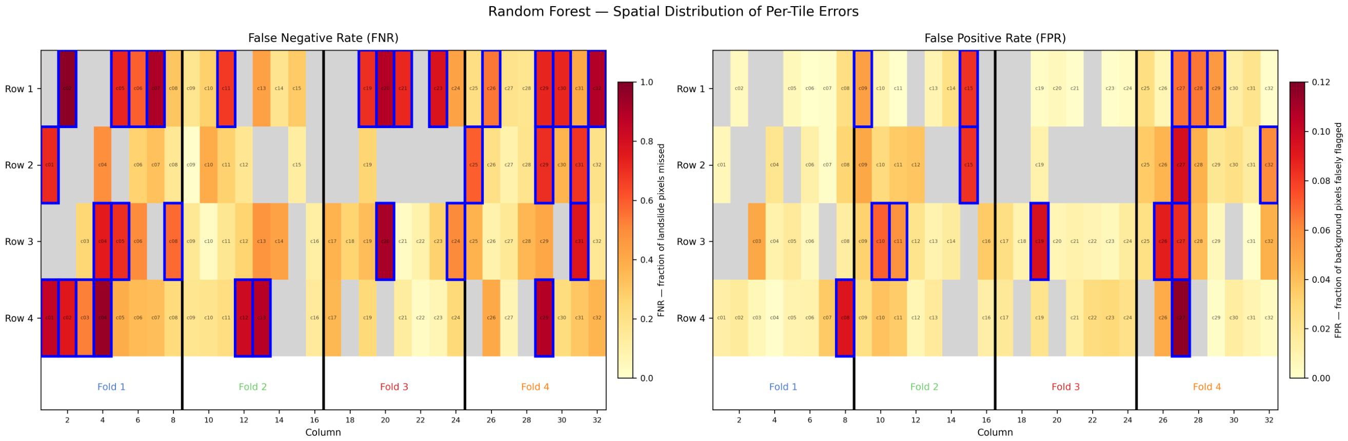
Per-tile FNR and FPR values showed substantial spatial heterogeneity across the 96 annotated landslide-containing tiles (Figure 12). The tile-weighted mean FNR was $0.400\pm 0.263$, which was higher than the pixel-weighted value of 0.319 because tiles with relatively few landslide pixels tended to have high miss rates and therefore exerted greater influence on the tile-weighted average. The tile-weighted mean FPR was $0.027\pm 0.026$, indicating a relatively low false-positive rate under the default classification threshold of 0.5. The maximum per-tile FPR observed was 0.117 (tile r04_c27, Fold 4). All per-tile error metrics were computed at the default classification threshold of 0.5; lower thresholds would be expected to reduce FNR at the cost of increased FPR. Because per-tile FNR and FPR values were computed from the same 3:1 sampled pixel subset used in model evaluation, the tile-weighted mean FNR is not directly comparable to fold-level recall, which is pixel-weighted across all sampled pixels in each fold.

Spatially, high-FNR tiles were concentrated in Row 1 across multiple columns (Figure 12), indicating that the northernmost strip of the annotated area was more difficult for the model under the present study design. Fold 1 showed the highest pixel-weighted FNR (0.460) compared with Folds 2–4 (0.259–0.285), consistent with the spatial error map showing elevated miss rates in columns 1–8. These patterns may reflect spatial variation in terrain character, vegetation cover, landslide size, landslide age, or image conditions, although these possibilities were not tested directly. FPR showed no strong spatial clustering, with relatively higher false-positive rates occurring in some tiles in columns 25–32 (Fold 4), where the model occasionally assigned landslide labels to bright background pixels adjacent to mapped landslide areas. The geographic basis of the elevated miss rates in Row 1 and Fold 1 remains uncertain and should be examined in future work.

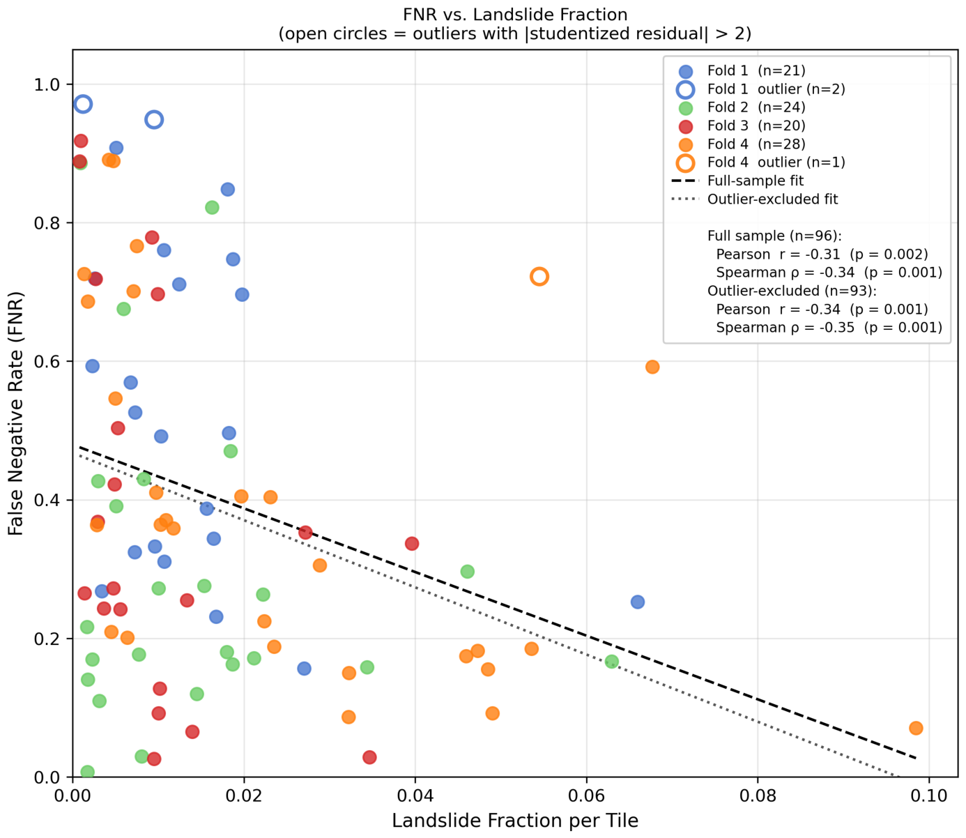
A statistically significant negative relationship was observed between per-tile landslide fraction and FNR ($r=-0.31$, $p=0.002$; Figure 13), indicating that tiles with smaller landslide extents tended to have higher miss rates in this dataset. This relationship was confirmed by Spearman’s rank correlation ($\rho =-0.34$, $p=0.001$), indicating robustness to non-normality, and by an outlier-sensitivity analysis: excluding three tiles flagged by externally studentized residuals (|residual| $>2$) slightly strengthened the association (Pearson $r=-0.34$, $p=0.001$; Spearman $\rho =-0.35$, $p=0.001$). Tiles with landslide fractions below approximately 0.01 often showed relatively high FNR values, with several exceeding 0.90. This pattern may reflect several factors, including the limited number of sampled landslide pixels in very small landslides, mixed-pixel boundary effects, and reduced spectral contrast relative to the surrounding terrain. In addition, some small landslides delineated using geomorphic-unit criteria may include partially revegetated or shadowed areas whose spectral characteristics are less distinct.

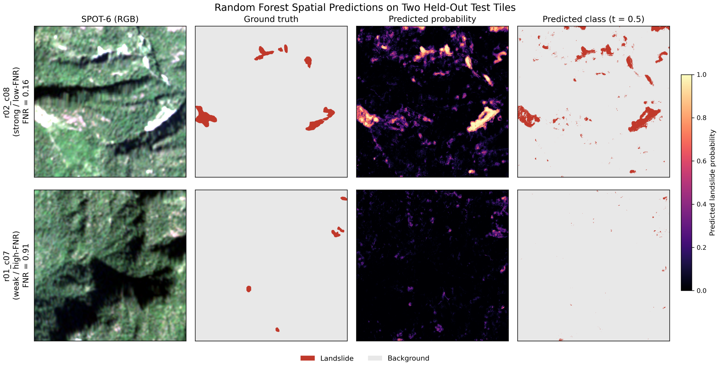
Figure 14 illustrates these spatial patterns directly, showing the Random Forest predictions on two held-out test tiles. In the strong case (tile r02_c08, FNR $=0.16$), the predicted probability field concentrates on the annotated landslide scars and recovers most landslide pixels at the default threshold, though a number of scattered false positives occur on bare surfaces that are spectrally similar to landslide scars, consistent with the tile’s false-positive rate of 0.03. In the difficult case (tile r01_c07, FNR $=0.91$), a Row 1 tile with a small landslide fraction, the annotated units are small and partially revegetated; they generate only weak predicted probabilities and are largely absent from the predicted class map at the default threshold. This example concretely illustrates the high-miss behavior associated with small and partially revegetated landslides discussed above, in which reduced spectral contrast against the vegetated background limits per-pixel detectability.

4.5. Classification Threshold Optimization

To assess sensitivity to the default classification threshold of 0.5, the threshold that maximized the F1 score was identified for each model and spatial fold from the precision–recall curve (Figure 4;

Table 5. Classification performance at the default threshold (0.5) and at the fold-optimized F1 threshold for each model. Values are mean ± standard deviation across four spatial folds. Optimal thresholds were identified from test-fold predictions and should be interpreted as optimistic upper bounds on threshold-optimized performance.

Model	Default F1	Optimal F1	$\mathbf{\Delta }$F1	Optimal Threshold
Logistic Regression	$0.772\pm 0.038$	$0.787\pm 0.044$	+0.014	$0.658\pm 0.190$
Random Forest	$0.755\pm 0.062$	$0.798\pm 0.038$	+0.042	$0.264\pm 0.070$
XGBoost	$0.775\pm 0.037$	$0.779\pm 0.037$	+0.004	$0.520\pm 0.145$

). Threshold optimization improved F1 for all three models. Random Forest showed the largest improvement, with mean F1 increasing from $0.755\pm 0.062$ to $0.798\pm 0.038$ ($\Delta =+0.042$) at a mean optimal threshold of $0.264\pm 0.070$, which is substantially below the default threshold of 0.5. At this threshold, Random Forest achieved a mean recall of 0.823 and a mean precision of 0.774, indicating a more balanced precision–recall trade-off than at the default threshold. Logistic Regression showed a smaller improvement ($\Delta$F1 $=+0.014$) with a higher mean optimal threshold ($0.658\pm 0.190$). XGBoost showed only a small gain from threshold optimization ($\Delta$F1 $=+0.004$), with a mean optimal threshold of $0.520\pm 0.145$. Among individual folds, Fold 1 showed the largest improvement for Random Forest ($\Delta$F1 $=+0.090$ at threshold $=0.190$), consistent with the greater classification difficulty of this spatial region identified in Section 4.4. These threshold-optimized results should be interpreted as a secondary sensitivity analysis rather than as primary model-comparison results.

To support application-specific threshold selection, the Random Forest classifier was evaluated across a range of decision thresholds to characterize two practically relevant operating points (

Table 6. Random Forest precision and recall at selected decision thresholds across two recommended operating point ranges. Values are mean ± standard deviation across four spatial folds. The default threshold of 0.5 is included for reference; the corresponding F1 score at this threshold is reported in Table 5.

Range	Threshold	Precision	Recall
High recall	0.20	0.738 ± 0.058	0.853 ± 0.060
High recall	0.25	0.767 ± 0.053	0.826 ± 0.068
High recall	0.30	0.790 ± 0.048	0.800 ± 0.074
Reference	0.50	0.858 ± 0.033	0.681 ± 0.095
High precision	0.60	0.883 ± 0.030	0.614 ± 0.100
High precision	0.65	0.895 ± 0.028	0.577 ± 0.102
High precision	0.70	0.907 ± 0.027	0.537 ± 0.101

). For a high-recall screening regime intended to capture the broadest possible set of candidate landslide pixels before manual review, thresholds in the range 0.20–0.30 yielded a mean recall of 0.853 ± 0.060 at a mean precision of 0.738 ± 0.058 (threshold = 0.20), declining to a mean recall of 0.800 ± 0.074 at a mean precision of 0.790 ± 0.048 (threshold = 0.30). This regime is appropriate when the primary concern is avoiding missed detections, while accepting a higher false-positive rate that downstream expert review can filter out. Conversely, for high-precision mapping in which confident positive predictions are required—for example, to seed automated delineation or provide reliable candidate annotations—thresholds in the range 0.60–0.70 achieved a mean precision of 0.883 ± 0.030 at a mean recall of 0.614 ± 0.100 (threshold = 0.60), increasing to a mean precision of 0.907 ± 0.027 at a mean recall of 0.537 ± 0.101 (threshold = 0.70). These results indicate that the choice of operating point should be guided by workflow context: lower thresholds maximize coverage for screening tasks, while higher thresholds provide sparser but more reliable positive predictions suitable for direct mapping or annotation-assistance applications. The two regimes thus serve complementary roles in sustainability-oriented hazard management: high-recall screening supports disaster risk reduction by minimizing missed detections, while high-precision mapping supports efficient and sustainable maintenance of landslide inventories. These operating-point ranges are reported for illustrative purposes only. All thresholds reported in this section, including the F1-maximizing thresholds in Table 5 and the application-specific ranges in Table 6, were identified from test-fold predictions and should therefore be regarded as optimistic upper bounds on threshold-optimized performance within the present study design. In practical application, threshold selection should be based on a separate validation set or another independent tuning procedure, rather than applying these values operationally without independent calibration.

4.6. Classification Probability Calibration

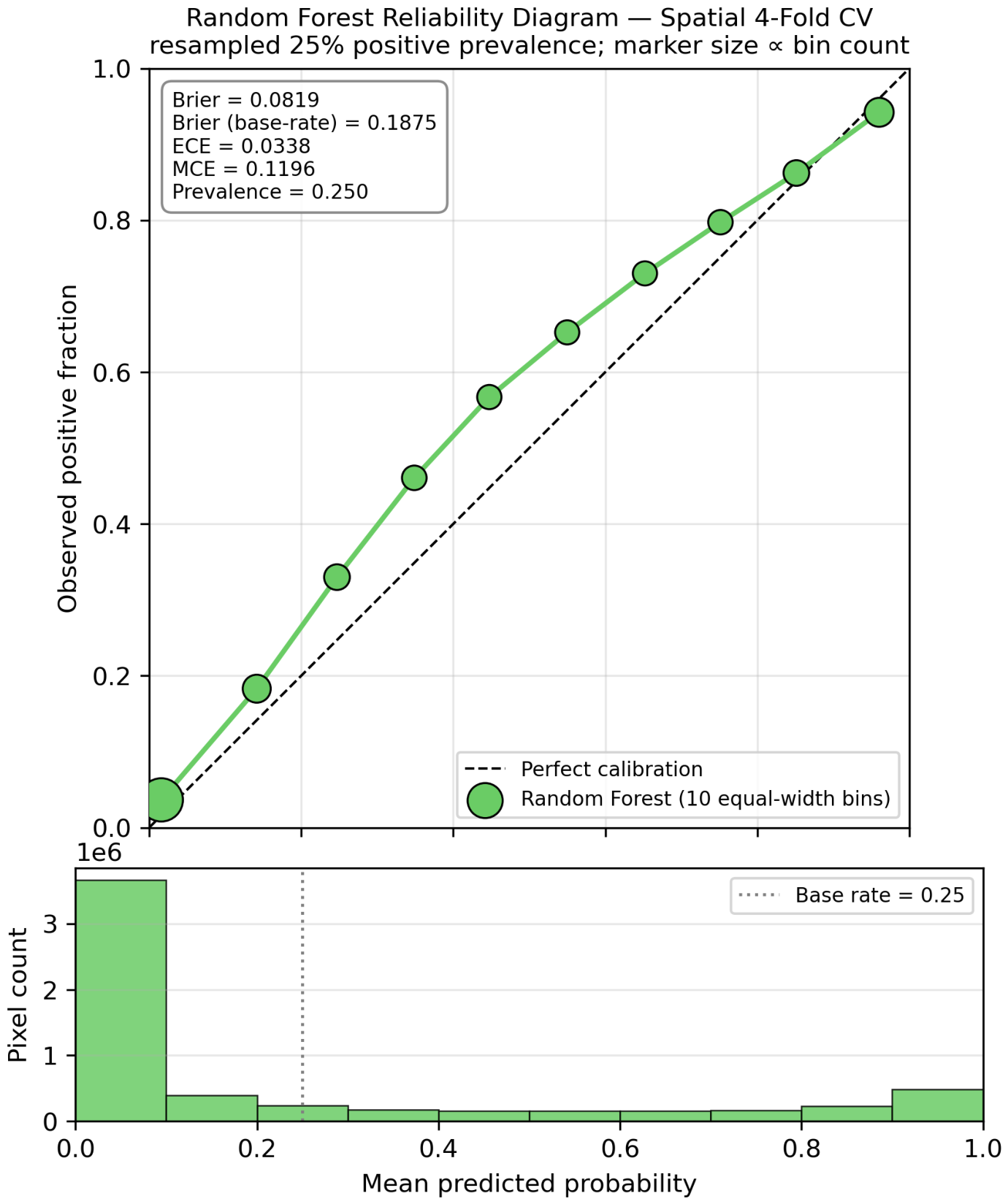
To characterize the reliability of the Random Forest probability estimates, we assessed calibration on the same 3:1 resampled evaluation distribution used throughout this study, pooling the out-of-fold test predictions across the four spatial folds. Because calibration is prevalence-dependent, these results describe calibration within the sampled evaluation setting (positive prevalence 25.0%) and should not be read as calibration under the natural class prevalence of the full watershed, which would differ. The Random Forest achieved a Brier score of 0.082, substantially better than the base-rate reference of 0.188 (a Brier skill score of 0.56), and an expected calibration error (ECE) of 0.034 over ten equal-width probability bins (0.041 ± 0.022 across folds), with a maximum calibration error of 0.120; quantile binning reproduced the same picture (ECE $=0.034$). The reliability diagram (Figure 15) shows that the model is predominantly under-confident across the mid-probability range, with the observed positive fraction lying above the predicted probability between approximately 0.05 and 0.85 and the largest deviation (≈0.12) near mid-range predictions; the model becomes marginally over-confident only in the highest probability bin. This under-confidence is consistent with the use of balanced class weights on the resampled distribution and is the same behavior reflected in the F1-optimal thresholds below 0.5 reported in Section 4.5, at which the lowered decision threshold compensates for the systematically conservative mid-range probabilities. As with all other metrics reported here, these calibration results are conditional on the resampled evaluation setting and the annotated pilot subregion.

5. Discussion

This section interprets the results of the pilot study in the context of the research objectives, the characteristics of the dataset, and the broader landslide-mapping literature. Section 5.1 discusses overall model performance and the implications of the precision–recall trade-off within the present experimental setting. Section 5.2 interprets the SHAP-identified feature contributions in relation to known landslide surface characteristics and the annotation framework. Section 5.3 addresses the principal limitations of the study. Section 5.4 outlines priorities for future work as annotation progresses toward the full 2048-tile dataset.

5.1. Model Performance in Context

All three classifiers achieved AP values between 0.846 and 0.858 under spatially blocked cross-validation, well above the no-skill baseline of 0.250 for the resampled evaluation dataset. These results are encouraging within the context of this 128-tile preliminary investigation and indicate that the combination of geomorphometric and spectral features provided useful discriminatory information for pixel-level landslide classification in the Laonung Creek Watershed. However, direct comparison with published studies remains difficult because reported performance depends strongly on spatial resolution, class balance, annotation methodology, and validation strategy. In particular, studies that do not apply spatially aware validation may report more optimistic results. The values reported here should therefore be interpreted within the present pilot-study design rather than as a universal benchmark.

The similar AP values observed across three models of differing complexity suggest that, under the present feature set and evaluation design, nonlinear models provided limited additional benefit over a linear baseline. This interpretation is consistent with the annotation protocol, in which current landslides were defined using optical evidence of bare-soil exposure or vegetation disturbance, characteristics that are also strongly reflected in variables such as the red band and NDVI. At the same time, this result should not be interpreted as proof that the landslide–background decision boundary is inherently “linear” in a broader sense. Rather, it indicates that, within this exploratory dataset and its feature representation, the dominant discriminatory signal was already captured effectively by relatively simple predictors. We emphasize that this convergence is a statement about model families evaluated under fixed, reasonable configurations, not a claim that any individual model was optimally tuned. In particular, XGBoost was run with an untuned default learning rate (Section 3.7), so its near-parity with the other models should not be read as its best achievable performance. The evidential weight of the convergence claim rests instead on the linear baseline and the single- and two-feature baselines of Section 4.1: logistic regression, which cannot exploit nonlinear structure, and a Band 3-only predictor both recover most of the available skill, and no amount of additional ensemble tuning can lower those baselines. This interpretation is now supported by a formal pairwise comparison (Section 4.1): the linear baseline is statistically indistinguishable in average precision from both tree ensembles, and the only statistically detectable pairwise difference, a ∼0.011 AP advantage of Random Forest over XGBoost, is too small to bear on any conclusion drawn here. A more thoroughly tuned XGBoost could raise its own AP but would not overturn this finding.

Under these conditions, feature representation and label definition may have mattered more to performance than model complexity. The tree-ensemble models evaluated here capture feature interactions implicitly, since each decision path represents a conjunction of feature thresholds; the absence of a performance advantage for these models over the linear baseline therefore indicates that feature interactions add little discriminatory power within this feature set, rather than that such interactions were unavailable to the models.

We note that the observed convergence could arise from any of three non-exclusive mechanisms: the relative simplicity and strong spectral separability of the present feature set, the coherence of the annotation protocol (in which optical bare-soil evidence provided the primary labeling cue, favoring spectral predictors), or the limited scale and geographic diversity of the four-row pilot subregion. Distinguishing among these mechanisms would require controlled reduced-feature-subset and regularization-path analyses; we identify this as a direction for future work once the annotated dataset is expanded.

An important constraint on the interpretation of all reported metrics is that the model was trained and evaluated exclusively on tiles containing landslides. It was never exposed to genuinely landslide-free terrain during training or evaluation. As a result, the reported false-positive rates reflect the model’s tendency to misclassify background pixels within landslide-containing tiles, not its behavior on clean terrain where landslides are entirely absent. False-positive rates in operational deployment on landslide-free terrain may therefore be higher than those reported here, and this uncertainty should be considered when assessing the operational generalizability of the trained models. We considered evaluating false-positive behavior directly on the 32 landslide-free tiles within the annotated region, but elected not to do so in the present pilot for two reasons. The landslide-free tiles were never processed into model-ready inputs under the sampling, feature-extraction, and normalization pipeline of Section 3, and, more fundamentally, treating an unannotated tile as a confirmed negative is not justified without a dedicated verification step, since the absence of a delineated polygon does not by itself establish that a tile is landslide-free. A false-positive rate computed against unverified negatives would be difficult to interpret, and we regard a properly verified clean-terrain evaluation as a distinct contribution best pursued at watershed scale rather than as an addition to this pilot. It is, accordingly, the top future-work priority identified in Section 6. The per-tile analysis nonetheless offers a concrete indication of where false positives are most likely to arise on clean terrain: the highest per-tile FPR values occurred where the model assigned landslide labels to bright background pixels spectrally similar to landslide scars (Section 4.4; maximum per-tile FPR of 0.117 on tile r04_c27). On genuinely landslide-free terrain, the analogous confusion would be expected over roads, dry riverbeds, and exposed bedrock, and this bare-surface ambiguity, rather than random error, is the most likely source of operational false positives. The companion study [49] reports that semantic segmentation produces more spatially coherent probability fields with fewer scattered off-target positives than the pixel-wise classifier, suggesting one practical route to mitigating this behavior at watershed scale.

The relative importance of false positive rate (FPR) and false negative rate (FNR) depends on the intended application. For hazard mapping or screening-oriented applications, lower FNR and higher recall are important because missed landslide pixels correspond to potentially overlooked hazardous areas. In this context, the mean pixel-weighted FNR of 0.319 for Random Forest indicates that approximately one-third of sampled landslide pixels were missed at the default classification threshold. By contrast, for landslide inventory construction and annotation assistance, which are closer to the intended use of this pilot study, high precision and low FPR may be more important because false positives can introduce erroneous mapped areas that require manual correction. Under the default threshold, the Random Forest model achieved a mean precision of 0.858 and a mean FPR of 0.027, indicating relatively few false-positive predictions in the sampled evaluation setting. As noted in Section 3.8, the recall and false-negative rate quoted here are prevalence-independent and carry over to the natural-prevalence setting, whereas the reported precision and FPR-linked advantages would weaken at the natural landslide prevalence of approximately 1.7%, where confident positive predictions become harder to sustain against a much larger background population; the precision reported here should therefore be regarded as an upper reference rather than an operational estimate. This operating point may therefore be useful for semi-automated annotation workflows in which model predictions are reviewed by an expert rather than accepted as a final mapping product. Users prioritizing higher recall may adopt a lower classification threshold and accept a corresponding reduction in precision, as illustrated by the precision–recall curves in Figure 4. Because these trade-offs were evaluated on the resampled dataset used in this study, they should not be interpreted directly as operational performance under full-watershed conditions.

For context, the companion deep learning study [49] reports that, on matched pixel positions from the same 29 held-out test tiles, the best U-Net configuration (multi-source six-channel input) achieves a matched-pixel AP of 0.847, compared with 0.824 for the Random Forest model reported here. The mean per-tile AP difference (DL − RF) is +0.019, a per-tile statistic that differs from the 0.023 gap between the pooled matched-pixel APs because per-tile averaging weights each test tile equally rather than by pixel count, with a bootstrap 95% confidence interval of [−0.034, +0.058] that crosses zero, indicating that neither approach is statistically superior at this test-set size.

Table 7. Key results from the companion U-Net study [49], reproduced here so that the comparison in Section 5.1 can be followed without consulting the companion paper. Matched-pixel AP values are computed on the stratified pixel sample shared with the present study and are elevated relative to full-tile AP; they are therefore not directly comparable to the full-tile input-modality AP values in the lower panel. All values are as reported in the published companion study, including the matched-pixel AP of the present study’s Random Forest model, which was evaluated there on the shared test tiles.

Quantity	Value
Matched-pixel comparison (RF vs. U-Net, 29 shared test tiles)
Random Forest matched-pixel AP (this study)	0.824
U-Net matched-pixel AP (Input D, companion)	0.847
Mean per-tile AP difference (DL − RF)	+0.019
Bootstrap 95% CI of per-tile difference	[−0.034, +0.058]
U-Net full-tile test AP by input modality (companion)
Input A—fused DEM–optical composite	0.511
Input B—SPOT-6 natural color (spectral only)	0.263
Input C—DEM stack (terrain only)	0.152
Input D—multi-source six-channel stack	0.556

summarizes these matched-pixel figures together with the companion study’s full-tile input-modality AP values, so that the comparison drawn here can be followed without consulting the companion paper directly; note that the matched-pixel AP values are elevated relative to full-tile AP and the two sets of figures are not directly comparable. This comparison suggests that learned convolutional representations achieve pixel-level classification performance comparable to carefully engineered spectral and topographic features, while additionally producing spatially coherent probability maps that capture landslide geomorphic-unit boundaries more directly than pixel-wise classifiers. Readers are directed to the companion study for a full discussion of the methodological trade-offs between pixel-wise feature engineering and deep learning segmentation.

Beyond these performance considerations, the classification outputs connect to sustainability objectives in several concrete ways. First, spatially explicit maps of current landslide extent provide a direct input to land-degradation monitoring under Sustainable Development Goal 15 (Life on Land): landslide scars represent a form of land degradation relevant to indicator SDG 15.3.1 (the proportion of land that is degraded), and repeated mapping supports tracking of both new disturbance and subsequent revegetation as an indicator of ecosystem recovery. Second, the per-tile probability maps, combined with the high-precision operating point characterized in Section 4.5, can be used to rank slopes, sub-catchments, and infrastructure corridors for restoration and slope-stabilization investment, helping watershed managers allocate limited resources toward the areas of greatest need. Third, in the context of climate adaptation, repeated post-event mapping supports monitoring of landslide reactivation and vegetation recovery over time, informing adaptation planning as the frequency and intensity of triggering typhoon rainfall change. These applications should be understood as prospective uses of the mapping framework rather than as capabilities demonstrated by the present pilot, which remains methodologically informative rather than deployment-ready; realizing them will require the watershed-scale extension and negative-tile evaluation discussed above.

5.2. Physical Interpretation of Feature Contributions

The prominence of SPOT-6 Band 3 (Red) and NDVI across the tree-based models is consistent with the characteristics of the annotated landslide surfaces in this study. Fresh landslide scars commonly expose mineral soil and weathered rock with relatively high red-band reflectance, whereas the surrounding forested hillslopes generally maintain stronger vegetation signals and more positive NDVI values. This spectral contrast is also consistent with the annotation protocol, in which optical imagery served as the primary basis for identifying current landslide activity.

The modest but non-negligible contribution of topographic features, particularly DEM elevation and slope, is consistent with the role of DEM information in the annotation workflow, where it was used mainly to refine boundaries and confirm geomorphic context rather than to identify landslides independently. The weak contribution of curvature at the pixel level is physically plausible and reflects three compounding factors. First, curvature is a second derivative of elevation, and second-derivative computation amplifies DEM errors quadratically with decreasing pixel spacing. At very high resolution, even minor surface roughness or positional uncertainty in the DEM can produce large curvature artifacts that obscure the geomorphically meaningful signal. Second, single-pixel curvature at very high resolution captures microtopographic roughness—rock outcrops, tree-throw pits, and minor rilling—rather than the concave–convex morphology of landslide scarps and accumulation zones that is relevant to geomorphic unit delineation. Third, curvature is most informative as a landslide predictor when computed over a neighborhood window matched to the scale of the geomorphic feature of interest, typically tens to hundreds of meters. Computing curvature at the native pixel scale is therefore poorly matched to the spatial scale of the landslide boundaries targeted by the annotation protocol. Multi-scale curvature computation, or DEM smoothing before curvature derivation, may produce a more discriminative feature in future work.

The difference in feature concentration between RF and XGBoost indicates that the two models relied on the available predictors in different ways. XGBoost placed much greater emphasis on Band 3, whereas RF distributed importance more broadly across spectral bands, spectral indices, and selected topographic variables. This contrast may be relevant when considering model behavior under varying acquisition conditions, but the feature-contribution results presented here do not by themselves establish that one model is more robust than the other.

Taken together, and supported by SHAP analysis across all four spatial folds, the SHAP results indicate that the Random Forest model relied primarily on spectral patterns associated with high red reflectance and low vegetation-index values, with additional contributions from topographic variables such as slope. These patterns are consistent with the characteristics of the annotated landslide surfaces in the present pilot dataset. At the same time, they should be interpreted in light of the annotation protocol, which used optical evidence of recent bare-soil exposure as the primary basis for delineating current landslide activity. The cross-fold analysis confirmed that this importance structure is stable across spatial blocks: SPOT-6 Band 3 was the most influential feature in every fold, and NDVI was a consistent secondary predictor. The specific second-ranked feature, and DEM elevation in particular, varied across folds, so the detailed ordering below the two leading spectral predictors should be regarded as fold-dependent rather than fixed.

5.3. Limitations and Interpretive Caveats

The results of this study should be interpreted in light of three overarching constraints. First, model training and evaluation were conducted using a resampled pixel distribution (3:1 negative-to-positive ratio) within annotated tiles rather than the natural class prevalence of the full watershed; all reported AP, precision, recall, F1, and threshold trade-offs therefore reflect this sampled evaluation setting. Second, the annotated dataset is spatially restricted to a four-row pilot subregion of the Laonung Creek Watershed, and the results should not be assumed to generalize to other parts of the watershed or to other geographic settings without further validation. Third, all 96 tiles used for model training and evaluation contain landslides, meaning that the model was trained to distinguish landslide pixels from background pixels within positive tiles rather than from entirely landslide-free terrain; this limits the extent to which the reported results can be interpreted as direct evidence of full-watershed screening performance. Beyond these three overarching constraints, several additional factors limit the interpretation and generalizability of the present results, as discussed below.

First, landslide annotations reflect geomorphic-unit boundaries as interpreted by a single annotator team using a consistent but still subjective protocol; label uncertainty arising from interpreter judgment and SAM-assisted boundary fitting was not quantified in this study. Landslide boundary delineation is known to be interpreter-dependent, particularly along the transitional margins between failed and stable terrain for larger or partially revegetated units, and independent mappers can produce appreciably different delineations of the same event, leading to cartographic mismatch [16]. This form of label uncertainty is most consequential precisely where the model was least reliable: the small landslides (landslide fraction below approximately 0.01) that exhibited the highest false-negative rates, and the partially revegetated, low-contrast units whose boundaries are inherently the most ambiguous to delineate. Because the same expert annotations serve as both the training targets and the evaluation reference, boundary-level label noise propagates into both training and assessment; the reported metrics should therefore be interpreted as conditional on this single-protocol interpretation rather than as agreement-validated ground truth, and the per-tile metrics for the smallest and most revegetated landslides should be regarded as the most uncertain. A formal inter-annotator agreement study on a representative subset of tiles is identified as a priority for future work (Section 5.4). Second, the SPOT-6 imagery represents a partial temporal composite of two acquisition dates (13 January 2025 and 17 September 2024), whereas the DEM corresponds to a 2024 epoch, introducing temporal mismatch between the optical and topographic datasets. In addition, the two SPOT-6 acquisition dates span different seasons, with January corresponding to the dry season and September to the late typhoon season. This seasonal difference may introduce tile-level inconsistency in vegetation-sensitive indices such as NDVI and SAVI that is unrelated to landslide presence. We did not perform a direct statistical comparison of NDVI between the January-sourced and September-sourced tiles, because the two groups are not spatially matched: September imagery was used specifically where the January acquisition was cloud-affected, so the two sets differ in location, terrain, and land cover as well as in season, and an unmatched contrast would confound the seasonal signal with these underlying landscape differences. We note, however, that the seasonal concern bears mainly on the secondary spectral predictors: the study’s dominant and most robust predictor is SPOT-6 Band 3 (Red), which reflects bare-soil and exposed-rock brightness and is considerably less sensitive to seasonal vegetation phenology than NDVI or SAVI, whereas NDVI enters as a stable but secondary feature. A seasonal inconsistency in the vegetation indices would therefore be unlikely to overturn the Band 3-led result, which is consistent across all three models and all four spatial folds. A rigorous assessment of the seasonal effect would require matched-location acquisitions of the same tiles in both seasons, and is identified as a direction for future work (Section 5.4). Third, although the SHAP analysis was extended to all four spatial folds, the detailed directional and interaction analyses (beeswarm and dependence plots) are presented for a single held-out fold as a representative case; the beeswarm and dependence patterns for the remaining folds were not examined in comparable detail. Fourth, the absence of shortwave infrared bands in SPOT-6 limits the spectral discrimination of some bare-soil and rock surfaces that may be better separated with longer-wavelength data.

A further limitation of the pixel-based classification approach used in this study is that each pixel is classified independently, without reference to the spatial relationships, shape characteristics, or boundary coherence of neighboring pixels. This pixel-wise formulation can produce spatially fragmented prediction maps in which isolated pixels are classified differently from their immediate neighbors, generating salt-and-pepper noise that does not reflect the coherent spatial extent of landslide geomorphic units. Object-based image analysis partially addresses this limitation by grouping pixels into spatially homogeneous segments before classification, thereby incorporating local shape and texture context [48]. Deep learning semantic segmentation approaches, such as the U-Net architecture, learn spatially coherent representations directly from image patches and have been shown to produce smoother and more geomorphically plausible probability maps than pixel-wise classifiers for landslide mapping [57]. The companion deep learning study [49] explicitly addresses the spatial-coherence advantage of U-Net segmentation over pixel-wise classification on the same annotated dataset and provides a direct visual and quantitative comparison of the two approaches on the held-out test tiles.

5.4. Implications for Future Work

The results of this pilot study suggest several priorities for subsequent research. As annotation progresses toward the full 2048-tile dataset, the spatial extent of the training data will expand to include terrain types, landslide sizes, and vegetation conditions not represented in the current four-row subregion. Re-evaluation under a broader spatial extent should provide a stronger basis for assessing generalization within the Laonung Creek Watershed. The prominence of red-band reflectance and NDVI in the present analysis suggests that future feature engineering may benefit from incorporating temporally comparative spectral information to better distinguish recent landslide surfaces from older or more revegetated terrain. A formal inter-annotator agreement study, in which a representative subset of tiles is independently re-annotated by a second expert and boundary-level agreement is quantified (for example, using intersection over union or the F1 overlap between independent delineations), would allow the label uncertainty discussed in Section 5.3 to be characterized directly rather than discussed only in relation to the literature. Similarly, matched-location acquisitions of the same tiles in both the January dry season and the September typhoon season would allow the seasonal consistency of the vegetation-sensitive indices to be tested directly, resolving the acquisition-date confound identified in Section 5.3. A systematic hyperparameter optimization of the gradient-boosted model (varying the learning rate, tree depth, and regularization on a validation split drawn from the training folds, without reference to the held-out test data) would refine the magnitude of the cross-model performance comparison. As discussed in Section 5.1, the convergence finding itself does not rest on the gradient-boosted model being optimally configured and would not be affected. A controlled input modality ablation experiment comparing fused DEM–optical, spectral-only, terrain-only, and multi-source stacked inputs for U-Net semantic segmentation on the same annotated dataset is reported in the companion study [49], which evaluates feature contributions under the same spatially blocked design used here. Readers are directed to that study for input modality results that complement the pixel-level feature importance findings reported in the present paper.

6. Conclusions

This study developed a methodological baseline for a machine learning framework for pixel-level landslide classification in the Laonung (Laonong) Creek Watershed, Taiwan, using high-resolution DEM derivatives and SPOT-6 multispectral imagery. Three classifiers—logistic regression, random forest, and XGBoost—were evaluated under spatially blocked four-fold cross-validation on 96 expert-annotated landslide-containing tiles, with expert-delineated landslide masks based on geomorphic-unit boundaries serving as the reference labels. All three models substantially outperformed the no-skill baseline for the resampled evaluation dataset, achieving mean average precision values of 0.846–0.858. Models of differing complexity, from the linear baseline to the two tree ensembles, achieved closely comparable average precision, indicating that most of the discriminatory signal in this pilot dataset was already captured by relatively simple spectral and topographic predictors. SHAP analysis conducted across all four spatial folds identified SPOT-6 Band 3 (Red) as the dominant predictor in every fold, with NDVI a consistent secondary predictor, consistent with the spectral characteristics of the annotated landslide surfaces in this dataset and with the annotation protocol, which used optical evidence as the primary basis for identifying current landslide activity.

Per-tile error analysis showed a significant negative relationship between landslide fraction and false negative rate ($r=-0.31$, $p=0.002$), indicating that smaller landslide extents tended to be associated with higher miss rates in the present dataset. This result suggests that very small landslides may be more difficult to detect under a per-pixel classification framework. Nevertheless, the findings of this study should be interpreted in light of several important constraints: the analysis was limited to a pilot subregion of the watershed, the modeled tiles all contained landslides, and model training and evaluation were conducted on a resampled pixel distribution rather than on the natural class prevalence of the full watershed.

Within these limits, this study provides a transferable and methodologically transparent exploratory baseline for subsequent landslide classification analysis in the Laonung Creek Watershed as annotation progresses toward the full 2048-tile dataset. Among the findings reported here, those considered most robust are the dominance of SPOT-6 Band 3 as the leading predictor, which is physically well grounded and consistent across all three models and all four spatial folds, with NDVI a consistent secondary predictor, and the negative relationship between landslide fraction and false negative rate (r = −0.31, p = 0.002), which has a clear physical interpretation and is supported by the full set of 96 tiles. A cross-fold SHAP analysis confirmed that this importance structure is stable across spatial blocks (pairwise Spearman rank correlations of 0.86–0.96), while also showing that the ordering of features below the two leading spectral predictors, and the rank of DEM elevation in particular, varies by spatial block. Findings that require further validation include the linear–nonlinear performance convergence, which may reflect the limited geographic diversity of the four-row pilot subregion rather than a general property of the feature space. The statistical reliability of all reported metrics is directly constrained by the small annotated dataset of 96 tiles. With this sample size, performance differences among models are within one standard deviation of each other, and conclusions about relative model superiority should be treated as indicative rather than definitive. Future research should prioritize, in order of expected impact, the following: (i) expanding annotation coverage to include additional watershed rows and landslide-free tiles to enable rotating spatial cross-validation and characterization of false-positive behavior on clean terrain, and (ii) evaluating whether ensemble or modality-adaptive approaches combining pixel-wise and deep learning predictions can improve detection of small landslides, which showed the highest miss rates in the present study.

References

1. Dadson, S.J.; Hovius, N.; Chen, H.; Dade, W.B.; Lin, J.-C.; Hsu, M.-L.; Lin, C.-W.; Horng, M.-J.; Chen, T.-C.; Milliman, J.; et al. Earthquake-triggered increase in sediment delivery from an active mountain belt. Geology 2004, 32, 733–736. [Google Scholar] [CrossRef]
2. Tsai, F.; Lai, J.-S.; Chen, W.W.; Lin, T.-H. Analysis of topographic and vegetative factors with data mining for landslide verification. Ecol. Eng. 2013, 61, 669–677. [Google Scholar] [CrossRef]
3. Nguyen, K.A.; Jiang, Y.-J.; Chen, W. Identifying Slope Hazard Zones in Central Taiwan Using Emerging Hot Spot Analysis and NDVI. Sustainability 2025, 17, 7428. [Google Scholar] [CrossRef]
4. Nguyen, K.A.; Huang, C.-S.; Chen, W. Machine Learning-Based Land Cover Mapping of Nanfeng Village with Emphasis on Landslide Detection. Sustainability 2025, 17, 8250. [Google Scholar] [CrossRef]
5. Shen, Z.-P.; Chen, W.W. Profile orientation and slope stability analysis. Sci. Program. 2016, 2016, 7029786. [Google Scholar] [CrossRef]
6. Capart, H.; Hsu, J.P.C.; Lai, S.Y.J.; Hsieh, M.-L. Formation and decay of a tributary-dammed lake, Laonong River, Taiwan. Water Resour. Res. 2010, 46, 1–23. [Google Scholar] [CrossRef]
7. Lo, C.-M. Evolution of deep-seated landslide at Putanpunas stream, Taiwan. Geomat. Nat. Hazards Risk 2017, 8, 1204–1224. [Google Scholar] [CrossRef]
8. Lo, C.-M.; Weng, M.-C.; Lin, M.-L.; Lee, S.-M.; Lee, K.-C. Landscape evolution characteristics of large-scale erosion and landslides at the Putanpunas Stream, Taiwan. Geomat. Nat. Hazards Risk 2018, 9, 175–195. [Google Scholar]
9. Tsai, F.; Hwang, J.-H.; Chen, L.-C.; Lin, T.-H. Post-disaster assessment of landslides in southern Taiwan after 2009 Typhoon Morakot using remote sensing and spatial analysis. Nat. Hazards Earth Syst. Sci. 2010, 10, 2179–2190. [Google Scholar] [CrossRef]
10. Chen, C.-Y. Landslide and debris flow initiated characteristics after Typhoon Morakot in Taiwan. Landslides 2016, 13, 153–164. [Google Scholar] [CrossRef]
11. Wu, C. Comparison and evolution of extreme rainfall-induced landslides in Taiwan. ISPRS Int. J. Geo-Inf. 2017, 6, 367. [Google Scholar] [CrossRef]
12. Lai, J.-S. Separating landslide source and runout signatures with topographic attributes and data mining to increase the quality of landslide inventory. Appl. Sci. 2020, 10, 6652. [Google Scholar] [CrossRef]
13. Lai, J.-S.; Chiang, S.-H.; Tsai, F. Exploring influence of sampling strategies on event-based landslide susceptibility modeling. ISPRS Int. J. Geo-Inf. 2019, 8, 397. [Google Scholar] [CrossRef]
14. Lai, J.-S.; Tsai, F. Improving GIS-based landslide susceptibility assessments with multi-temporal remote sensing and machine learning. Sensors 2019, 19, 3717. [Google Scholar] [CrossRef] [PubMed]
15. Pardeshi, S.D.; Autade, S.E.; Pardeshi, S.S. Landslide hazard assessment: Recent trends and techniques. SpringerPlus 2013, 2, 523. [Google Scholar] [CrossRef] [PubMed]
16. Guzzetti, F.; Mondini, A.C.; Cardinali, M.; Fiorucci, F.; Santangelo, M.; Chang, K.-T. Landslide inventory maps: New tools for an old problem. Earth-Sci. Rev. 2012, 112, 42–66. [Google Scholar] [CrossRef]
17. Okoli, J.; Nahazanan, H.; Nahas, F.; Kalantar, B.; Shafri, H.Z.M.; Khuzaimah, Z. High-resolution lidar-derived DEM for landslide susceptibility assessment using AHP and fuzzy logic in Serdang, Malaysia. Geosciences 2023, 13, 34. [Google Scholar] [CrossRef]
18. Chu, H.-J.; Wang, C.-K.; Huang, M.-L.; Lee, C.-C.; Liu, C.-Y.; Lin, C.-C. Effect of point density and interpolation of LiDAR-derived high-resolution DEMs on landscape scarp identification. GISci. Remote Sens. 2014, 51, 731–747. [Google Scholar] [CrossRef]
19. Andualem, T.G.; Peters, S.; Hewa, G.A.; Myers, B.R.; Boland, J.; Pezzaniti, D. Channel morphological change monitoring using high-resolution LiDAR-derived DEM and multi-temporal imageries. Sci. Total Environ. 2024, 921, 171104. [Google Scholar] [CrossRef] [PubMed]
20. Shen, D.; Wang, J.; Cheng, X.; Rui, Y.; Ye, S. Integration of 2-D hydraulic model and high-resolution lidar-derived DEM for floodplain flow modeling. Hydrol. Earth Syst. Sci. 2015, 19, 3605–3616. [Google Scholar] [CrossRef]
21. Muhadi, N.A.; Abdullah, A.F.; Bejo, S.K.; Mahadi, M.R.; Mijic, A. The use of LiDAR-derived DEM in flood applications: A review. Remote Sens. 2020, 12, 2308. [Google Scholar] [CrossRef]
22. Mondini, A.C.; Marchesini, I.; Rossi, M.; Chang, K.-T.; Pasquariello, G.; Guzzetti, F. Bayesian framework for mapping and classifying shallow landslides exploiting remote sensing and topographic data. Geomorphology 2013, 201, 135–147. [Google Scholar] [CrossRef]
23. Sameen, M.I.; Pradhan, B. Landslide detection using residual networks and the fusion of spectral and topographic information. IEEE Access 2019, 7, 114363–114373. [Google Scholar] [CrossRef]
24. Rau, J.-Y.; Jhan, J.-P.; Rau, R.-J. Semiautomatic object-oriented landslide recognition scheme from multisensor optical imagery and DEM. IEEE Trans. Geosci. Remote Sens. 2013, 52, 1336–1349. [Google Scholar]
25. Pradhan, B.; Jebur, M.N.; Shafri, H.Z.M.; Tehrany, M.S. Data fusion technique using wavelet transform and Taguchi methods for automatic landslide detection from airborne laser scanning data and QuickBird satellite imagery. IEEE Trans. Geosci. Remote Sens. 2015, 54, 1610–1622. [Google Scholar] [CrossRef]
26. Miura, H. Fusion analysis of optical satellite images and digital elevation model for quantifying volume in debris flow disaster. Remote Sens. 2019, 11, 1096. [Google Scholar] [CrossRef]
27. Pradhan, B.; Al-Najjar, H.A.H.; Sameen, M.I.; Mezaal, M.R.; Alamri, A.M. Landslide detection using a saliency feature enhancement technique from LiDAR-derived DEM and orthophotos. IEEE Access 2020, 8, 121942–121954. [Google Scholar] [CrossRef]
28. Ren, Z.; Ma, J.; Liu, J.; Deng, X.; Zhang, G.; Guo, H. Enhancing deep learning-based landslide detection from open satellite imagery via multisource data fusion of spectral, textural, and topographical features: A case study of old landslide detection in the Three Gorges Reservoir Area (TGRA). Geocarto Int. 2024, 39, 2421224. [Google Scholar] [CrossRef]
29. Zhou, X.; Wen, H.; Zhang, Y.; Xu, J.; Zhang, W. Landslide susceptibility mapping using hybrid random forest with GeoDetector and RFE for factor optimization. Geosci. Front. 2021, 12, 101211. [Google Scholar] [CrossRef]
30. Kavzoglu, T.; Teke, A. Predictive performances of ensemble machine learning algorithms in landslide susceptibility mapping using random forest, extreme gradient boosting (XGBoost) and natural gradient boosting (NGBoost). Arab. J. Sci. Eng. 2022, 47, 7367–7385. [Google Scholar] [CrossRef]
31. Rong, G.; Alu, S.; Li, K.; Su, Y.; Zhang, J.; Zhang, Y.; Li, T. Rainfall induced landslide susceptibility mapping based on Bayesian optimized random forest and gradient boosting decision tree models—A case study of Shuicheng County, China. Water 2020, 12, 3066. [Google Scholar] [CrossRef]
32. Sahin, E.K. Comparative analysis of gradient boosting algorithms for landslide susceptibility mapping. Geocarto Int. 2022, 37, 2441–2465. [Google Scholar] [CrossRef]
33. Sahin, E.K. Assessing the predictive capability of ensemble tree methods for landslide susceptibility mapping using XGBoost, gradient boosting machine, and random forest. SN Appl. Sci. 2020, 2, 1308. [Google Scholar] [CrossRef]
34. Shahzad, N.; Ding, X.; Abbas, S. A comparative assessment of machine learning models for landslide susceptibility mapping in the rugged terrain of northern Pakistan. Appl. Sci. 2022, 12, 2280. [Google Scholar] [CrossRef]
35. Brenning, A. Spatial prediction models for landslide hazards: Review, comparison and evaluation. Nat. Hazards Earth Syst. Sci. 2005, 5, 853–862. [Google Scholar] [CrossRef]
36. Brenning, A. Spatial machine-learning model diagnostics: A model-agnostic distance-based approach. Int. J. Geogr. Inf. Sci. 2023, 37, 584–606. [Google Scholar]
37. Dai, X.; Zhu, Y.; Sun, K.; Zou, Q.; Zhao, S.; Li, W.; Hu, L.; Wang, S. Examining the spatially varying relationships between landslide susceptibility and conditioning factors using a geographical random forest approach: A case study in Liangshan, China. Remote Sens. 2023, 15, 1513. [Google Scholar] [CrossRef]
38. Kopczewska, K. Spatial machine learning: New opportunities for regional science. Ann. Reg. Sci. 2022, 68, 713–755. [Google Scholar]
39. Rüther, D.C.; Haualand, K.F.; Peeters, I.L.J.; Gillespie, M.A.K. Spatial machine learning modelling reveals that soil indicators and tree type best explain shallow landslide release. EGUsphere 2026, 2026, 1–49. [Google Scholar] [CrossRef]
40. Sun, D.; Chen, D.; Zhang, J.; Mi, C.; Gu, Q.; Wen, H. Landslide susceptibility mapping based on interpretable machine learning from the perspective of geomorphological differentiation. Land 2023, 12, 1018. [Google Scholar] [CrossRef]
41. Collini, E.; Palesi, L.A.I.; Nesi, P.; Pantaleo, G.; Nocentini, N.; Rosi, A. Predicting and understanding landslide events with explainable AI. IEEE Access 2022, 10, 31175–31189. [Google Scholar] [CrossRef]
42. Dwivedi, A.; Congress, S.S.C.; Velasquez, R.; Kumar, P.; Patil, U. Explainable AI (xAI) for landslide susceptibility modeling: A comparative analysis of machine learning and deep learning approaches. Earth Syst. Environ. 2026, 1–33. [Google Scholar] [CrossRef]
43. Pradhan, B.; Dikshit, A.; Lee, S.; Kim, H. An explainable AI (XAI) model for landslide susceptibility modeling. Appl. Soft Comput. 2023, 142, 110324. [Google Scholar] [CrossRef]
44. Zhang, J.; Ma, X.; Zhang, J.; Sun, D.; Zhou, X.; Mi, C.; Wen, H. Insights into geospatial heterogeneity of landslide susceptibility based on the SHAP-XGBoost model. J. Environ. Manag. 2023, 332, 117357. [Google Scholar] [CrossRef]
45. Zhong, C.; Liu, Y.; Gao, P.; Chen, W.; Li, H.; Hou, Y.; Nuremanguli, T.; Ma, H. Landslide mapping with remote sensing: Challenges and opportunities. Int. J. Remote Sens. 2020, 41, 1555–1581. [Google Scholar]
46. Chen, X.; Li, W.; Hsu, C.-Y.; Arundel, S.T.; Higman, B. Harnessing geospatial artificial intelligence and deep learning for landslide inventory mapping: Advances, challenges, and emerging directions. Remote Sens. 2025, 17, 1856. [Google Scholar] [CrossRef]
47. Wang, Z.; Brenning, A. Active-learning approaches for landslide mapping using support vector machines. Remote Sens. 2021, 13, 2588. [Google Scholar] [CrossRef]
48. Amatya, P.; Kirschbaum, D.; Stanley, T.; Tanyas, H. Landslide mapping using object-based image analysis and open source tools. Eng. Geol. 2021, 282, 106000. [Google Scholar] [CrossRef]
49. Chen, W.; Tsai, F. Input Modality Ablation for Sustainable Landslide Hazard Management Using U-Net: Fused DEM–Optical vs. Spectral vs. Terrain Representations in a Small-Sample Pilot Study. Sustainability 2026, 18, 6649. [Google Scholar] [CrossRef]
50. Lundberg, S.M.; Lee, S.I. A unified approach to interpreting model predictions. Adv. Neural Inf. Process. Syst. 2017, 30, 4765–4774. [Google Scholar]
51. Chen, C.-H.; Lin, C.-W.; Chen, M.-M.; Chang, W.-S.; Liu, S.-H. A Landslide Study by Using Multi-Temporal Satellite Images: An Example from Lao-Lung River Watershed. J. Taiwan Disaster Prev. Soc. 2011, 3, 25–38. [Google Scholar] [CrossRef]
52. Lin, S.-C.; Shen, S.-M.; You, M.-D. Illustrated Explanatory Manual of Geomorphological Map for Sediment-Related Hazards, Taoyuan District–Laonung River–001; Department of Geography, National Taiwan Normal University: Taipei, Taiwan, 2023. (In Chinese) [Google Scholar]
53. CVAT.ai Corporation. Computer Vision Annotation Tool (CVAT). Available online: https://www.cvat.ai/ (accessed on 1 April 2026).
54. Carion, N.; Gustafson, L.; Hu, Y.-T.; Debnath, S.; Hu, R.; Suris, D.; Ryali, C.; Alwala, K.V.; Khedr, H.; Huang, A.; et al. Sam 3: Segment anything with concepts. arXiv 2025, arXiv:2511.16719. [Google Scholar]
55. Pedregosa, F.; Varoquaux, G.; Gramfort, A.; Michel, V.; Thirion, B.; Grisel, O.; Blondel, M.; Prettenhofer, P.; Weiss, R.; Dubourg, V.; et al. Scikit-learn: Machine Learning in Python. J. Mach. Learn. Res. 2011, 12, 2825–2830. [Google Scholar]
56. Chen, T.; Guestrin, C. XGBoost: A scalable tree boosting system. In Proceedings of the 22nd ACM SIGKDD International Conference on Knowledge Discovery and Data Mining, San Francisco, CA, USA, 13–17 August 2016; pp. 785–794. [Google Scholar]
57. Ghorbanzadeh, O.; Crivellari, A.; Ghamisi, P.; Shahabi, H.; Blaschke, T. A comprehensive transferability evaluation of U-Net and ResU-Net for landslide detection from Sentinel-2 data: Case study areas from Taiwan, China, and Japan. Sci. Rep. 2021, 11, 14629. [Google Scholar] [CrossRef] [PubMed]
Figure 1. Geographic setting of the study area. The blue rectangle marks the extent of the 64 rows by 32 columns tile grid covering most of the Laonung (Laonong) Creek Watershed in southern Taiwan, and the red rectangle marks the pilot subregion (rows 1–4, columns 1–32) used in this study.
Sustainability 18 07779 g001
Figure 2. Spatial distribution of the 128 annotated tiles and the cross-validation fold assignments across the pilot subregion (rows 1–4, columns 1–32). The background shows the DEM-derived hillshade mosaic. Colored overlays indicate fold assignment: Fold 1 (blue, columns 1–8), Fold 2 (orange, columns 9–16), Fold 3 (green, columns 17–24), and Fold 4 (red, columns 25–32). Thick vertical lines mark fold boundaries.
Sustainability 18 07779 g002
Figure 3. Representative annotation workflow for tile r01_c24. The panels show the DEM-derived hillshade, SPOT-6 natural color composite (RGB = bands 3, 2, 1), fused annotation composite, and expert-delineated landslide mask. The mask reflects the interpreted geomorphic-unit extent rather than the spectral bare-soil boundary alone.
Sustainability 18 07779 g003
Figure 4. Precision–recall curves for the three classifiers under spatially blocked four-fold cross-validation. Faint lines show individual folds, bold lines show mean curves, and shaded bands indicate ±1 standard deviation. The dashed line marks the no-skill baseline for the resampled evaluation dataset, and filled circles indicate F1-maximizing thresholds estimated from the test-fold predictions. The inset magnifies the high-recall region (recall > 0.70), where the mean curves of the three models are most clearly separated and the F1-maximizing operating points are located.
Sustainability 18 07779 g004
Figure 5. Receiver operating characteristic (ROC) curves for the three classifiers under spatially blocked four-fold cross-validation. Faint lines show individual folds, bold lines show mean curves, and shaded bands indicate ±1 standard deviation. The diagonal dashed line represents the no-skill reference.
Sustainability 18 07779 g005
Figure 6. Radar chart comparing the three classifiers (logistic regression, random forest, and XGBoost) across the five performance metrics reported in Table 3: precision, recall, F1, ROC-AUC, and average precision (AP). Values are the means across the four spatial cross-validation folds. The radial axis spans 0.6–1.0 to make differences among the closely performing models legible. Random Forest shows the highest precision and lowest recall, logistic regression the highest recall and lowest precision, and XGBoost an intermediate, balanced profile; all three models converge at high ROC-AUC and AP.
Sustainability 18 07779 g006
Figure 7. Normalized confusion matrices for the three classifiers across four spatial test folds. Each cell displays the row-normalized proportion in bold, the raw sampled pixel count in parentheses, and the metric name in italics (Specificity, FPR, FNR, or Recall). All subplots share a consistent color scale from 0 to 1. Rows represent models (Logistic Regression, Random Forest, XGBoost), and columns represent spatial test folds (Fold 1: columns 1–8; Fold 2: columns 9–16; Fold 3: columns 17–24; Fold 4: columns 25–32). The matrices show that Random Forest maintained high background specificity across folds while exhibiting lower landslide recall in Fold 1 than in the other folds.
Sustainability 18 07779 g007
Figure 8. Mean feature importance for Random Forest (left, green) and XGBoost (right, red) across four spatial cross-validation folds. Error bars show the standard deviation across folds. Features are ordered according to Random Forest importance. SPOT-6 Band 3 (Red) is the most important feature in both models, accounting for approximately 21% of Random Forest importance and 57% of XGBoost importance. Random Forest distributes importance across several spectral and topographic variables, whereas XGBoost places much greater emphasis on Band 3 and, to a lesser extent, NDVI. Note that Random Forest importance is computed as the mean decrease in Gini impurity, whereas XGBoost importance is computed as normalized gain across all splits. These quantities are not directly numerically comparable across the two models, and the comparison is intended to reveal qualitative differences in feature use rather than differences in absolute importance magnitude.
Sustainability 18 07779 g008
Figure 9. Mean absolute SHAP values for all 13 features, computed for the Random Forest model across the four spatial folds. For each fold, the model was retrained on the other three folds and SHAP values were computed on a stratified subsample of 2000 pixels (1000 positive and 1000 negative) from the held-out fold. Bars show the across-fold mean and error bars indicate ± one across-fold standard deviation (sample standard deviation, computed across the four folds; this reflects both sampling and model variation across spatial blocks and is not a bootstrap confidence interval). Features are sorted in descending order of across-fold mean |SHAP|. Bar colors indicate feature category: brown = topographic (DEM-derived), blue = raw SPOT-6 bands, and green = spectral indices.
Sustainability 18 07779 g009
Figure 10. SHAP beeswarm summary plot for the Random Forest model, generated from a stratified sample of 1000 pixels in the fold 4 test set. Each point represents an individual pixel. The horizontal axis shows the SHAP value, with positive values contributing toward the landslide class and negative values contributing toward the background class. Point color represents the corresponding feature value, with red indicating high values and blue indicating low values. Features are ranked by mean absolute SHAP value.
Sustainability 18 07779 g010
Figure 11. SHAP dependence plots for the three most influential features overall (SPOT-6 Band 3 (Red), NDVI, and SPOT-6 Band 1 (Blue)) and the two most influential topographic features (slope and DEM elevation). The x-axis shows the original pre-standardization feature values, and the y-axis represents the corresponding SHAP value for each pixel. Point color represents the value of the feature with the strongest detected interaction: NDVI for Band 3, SPOT-6 Band 3 for NDVI, NDWI for Band 1, NDVI for slope, and SPOT-6 Band 4 for DEM elevation. Dashed horizontal lines mark SHAP = 0 . The symbol “#” denotes the sequential number of each displayed feature and does not necessarily indicate its overall feature-importance rank.
Sustainability 18 07779 g011
Figure 12. Spatial distribution of per-tile classification errors for the Random Forest model across the 4 × 32 pilot tile grid. (Left panel): false negative rate (FNR), defined as the fraction of sampled landslide pixels missed in each tile. (Right panel): false positive rate (FPR), defined as the fraction of sampled background pixels incorrectly classified as landslide. The two panels use independent color scales. The FNR panel spans the full 0–1.0 range, whereas the FPR panel uses a data-adaptive range of 0–0.12 (maximum observed per-tile FPR = 0.117 ), restoring visual differentiation among tiles in the FPR map. Gray cells indicate annotated tiles without landslides and are not included in the per-tile landslide error summaries. Thick vertical lines mark fold boundaries (Fold 1: columns 1–8, Fold 2: columns 9–16, Fold 3: columns 17–24, and Fold 4: columns 25–32). In the (Left panel), blue borders indicate tiles with FNR > 0.5, meaning that most landslide pixels were missed. In the (Right panel), blue borders indicate tiles with FPR > 0.05.
Sustainability 18 07779 g012
Figure 13. Relationship between per-tile landslide fraction and false negative rate (FNR) for the Random Forest model. Each point represents one annotated landslide-containing tile, and colors indicate the spatial fold. The dashed line shows the fitted linear trend (Pearson r = 0.31 , p = 0.002 , Spearman ρ = 0.34 , p = 0.001 ), indicating that smaller landslide fractions were associated with higher miss rates in this dataset. Open circles mark three tiles flagged as potential outliers (|externally studentized residual| > 2 ). The dotted line shows the linear fit with these tiles excluded (Pearson r = 0.34 , p = 0.001 , Spearman ρ = 0.35 , p = 0.001 ), confirming that the negative relationship is robust to these leverage points.
Sustainability 18 07779 g013
Figure 14. Random Forest spatial predictions on two held-out test tiles from Fold 1. Each row shows, from left to right, the SPOT-6 natural-color composite (RGB = bands 3, 2, 1), the expert-delineated ground-truth landslide mask, the predicted landslide probability (shared 0–1 color scale), and the predicted binary class at the default threshold of 0.5. The top row (tile r02_c08) is a representative strong case (FNR = 0.16 ): predicted probability concentrates on the annotated landslide scars and most landslide pixels are recovered at the default threshold, with some scattered false positives on spectrally similar bare surfaces outside the mask (per-tile FPR = 0.03 ). The bottom row (tile r01_c07) is a representative difficult case from Row 1 (FNR = 0.91 ): the annotated units are small and partially revegetated, produce only weak predicted probabilities, and are largely missed at the default threshold. Predictions are genuinely out-of-sample, generated by the Random Forest model trained on Folds 2–4. Panels are shown at tile-relative extent without axis ticks or scale bars.
Sustainability 18 07779 g014
Figure 15. Reliability diagram for the Random Forest model, computed on the 3:1 resampled evaluation distribution (25% positive prevalence) with out-of-fold test predictions pooled across the four spatial folds. (Top panel): observed positive fraction versus mean predicted probability over ten equal-width bins, with marker size proportional to bin count and the dashed line indicating perfect calibration; the curve lying above the diagonal indicates under-confidence. (Bottom panel): histogram of predicted probabilities, with the 0.25 base rate marked. Brier score, base-rate Brier score, expected calibration error (ECE), and maximum calibration error (MCE) are annotated. Calibration is prevalence-dependent, so these values characterize the resampled evaluation setting and would differ under the natural class prevalence of the full watershed.
Sustainability 18 07779 g015