Human Population, Power, and CO₂ Dynamics: The Positive Feedback Loop of Unsustainability

Abstract

Population growth is the most basic component of the physical production of a human society, driven by energetic throughput that feeds back to further growth. The expansion of our population and energy systems has significantly altered the climate system that enables human activities. The objective of this study is to show that the changes in the human population and atmospheric CO₂, over the last 220 years, can be understood through a sigmoid S-shaped dynamic model fueled by global power and its growth rate. This study analyzed the time series of population size and atmospheric concentration from 1800 to 2020 using a sigmoid model influenced by the power dynamics. Population growth was driven by two forces: the long-term increase in power use and the faster interdecadal changes in power growth rates, while the increase in atmospheric CO₂ concentration growth rate is driven by the long-term increase in global power. Our expansionary population dynamic is starting to reach its limits. Population size, atmospheric CO₂ concentration, and power (energy/time) were engaged in a positive feedback loop that explained the dynamics of our population system, making our present human societies increasingly vulnerable to collapse.

1. Introduction

Human economic systems have always depended on the transformation of materials and energy [1,2]. Industrial civilization is fundamentally rooted in the exploitation of unpaid work by photosynthetic organisms, which converted solar energy and stored it as fossil fuels over millions of years [3,4,5]. This reliance on power (energy/time) is central to understanding human population and economic growth [5].

From a thermodynamic perspective, population growth is the most fundamental component of the physical production of a human society [6]. Population growth is driven by energetic throughput, which feeds back to further growth [7,8,9]. The global population is an open system that literally lives off environmental resources and exports unusable energy and materials of low structure and high simplicity—in other words, entropy [10]. In consequence, this intrinsic expansive and interdependent dynamics could constrain the general sustainable development goals, in particular those related to the joint achievement of economic growth, decent work, innovation, and climate action.

We face a key challenge: the massive growth of human societies over the past two centuries. This global niche construction is driven by population dynamics, cultural evolution [11], and fossil fuel energy [12,13]. During the Industrial Revolution, population growth was linked with increased technological innovation, economic activity, and energy use [7,8,14,15]. As populations grew and new energy gradients were used, health and life expectancy improved, enabling further population growth. This created a feedback loop: growing populations increased demand for energy and technology, which, in turn, drove further innovation, greater access to resources, and greater environmental pressure. As a result, population and energy use continued to rise [16,17,18].

The idea that human population size could stimulate its own growth by accelerating innovations that increase the dissipation of energy gradients from nature was proposed more than 70 years ago [19]. As the population grows, more minds and labor contribute to technological advances and resource extraction, enabling greater use of energy and resources from the environment. Several studies have examined the positive relationship between population size and growth rates in humans [7,20,21,22,23,24]. Recent human population dynamics are best understood by considering this positive feedback loop: growth enables innovation and expansion, which allow the extraction of more resources, in turn fueling further population increases [9,11].

Population growth patterns in various prehistoric societies mirror those during the Industrial Revolution, indicating that this positive feedback loop has operated throughout much of human demographic history, from hunter-gatherers to modern industrial societies [25]. Notably, periods of rapid expansion appear as a “relay” phenomenon [21], with population trajectories following overlapping sigmoid (S-shaped) curves. Hyperbolic dynamics emerge as the envelope of these local curves, reflecting overall self-accelerated expansion.

The expansion of our population and energy system has significantly altered the ecosystems that supply all the materials and energy for human activity [26]. Human societies evolve to maximize usable power—net energy extracted per unit time—by selectively drawing more energy and doing more work, which creates a strong feedback loop [16,27,28] and makes these systems apparently unsustainable [4,11,29].

This article focuses on the relationship between the maximum power principle [29,30], nonequilibrium thermodynamics of growth [10,31,32], and population dynamics theory [33,34,35] to reveal how energy conversion processes have shaped human population dynamics and atmospheric CO₂ concentration over the past 220 years.

Thus, the aim is to show that the interconnected growth of population and atmospheric CO₂ can be better understood through a series of sigmoid S-shaped models fueled by power (energy/time) dynamics. This article proposes that hyperbolic growth patterns in the human population and atmospheric CO₂ concentrations result from an overlapping series of S-shaped trajectories, highlighting the feedback loop between power and population expansion as the central process.

2. Materials and Methods

I defined the system using time series from 1800 to 2020 for population size (N), power (P), and atmospheric CO₂ concentration (CO₂). The decadal human population estimates (N) for the period 1800–2020 were based on Our World in Data (https://ourworldindata.org/population-growth, accessed on 16 September 2025), and the human population data for the period 1950–2020 are from the UN POP in World Population Prospects 2020. The time series of power by year in Terawatts (Pw) corresponds to the data (https://ourworldindata.org/energy-production-consumption, accessed on 18 November 2025), which corresponds to the amount of total energy consumption measured in Terawatt-hours/year [36], which was converted into an estimation of annual mean power by dividing by the number of annual hours (8760 h). The data on atmospheric carbon dioxide (CO₂) concentration, measured as dry molar fraction (ppm), averaged over a calendar year, are from Antarctic ice core records for the period 1800–1850 [37] and from 1960 to 2020 at the Mauna Loa Observatory (https://gml.noaa.gov/webdata/ccgg/trends/co2/co2_annmean_mlo.txt, accessed on 16 June 2026).

The global population, mean annual power, and atmospheric CO₂ concentration growth rates were estimated as follows:

$$R_{ t}= log\left({\displaystyle \frac{x_{t+1}}{x_t}}\right),$$

(1)

x represents the corresponding estimates of annual human population size (N), mean annual power (Pw), and atmospheric CO₂ (CO₂) concentrations between decades. The complete dataset is provided in the electronic Supplementary Material (Table S1).

Coupled dynamics of the energy, human population, and atmospheric CO₂.

When the cooperative social and technological pattern of self-accelerating development began, humans began to spread throughout the world, and their population grew well beyond that of any other comparable species. Global human population dynamics over the last 220 years can be considered a process of growth that, by using available energy reserves, can expand into new reserves of materials and energy; this expansion creates positive feedback that further accelerates population growth [7,8].

A key characteristic of historical human population dynamics data is a tendency toward hyper-exponential population growth [19,20,21,22,23,24]. This kind of population process has been derived in the literature in several different ways. Cohen [38] (1995) proposed two coupled Malthus-Condorcet equations for the human population by arguing that human carrying capacity increases with population size. In population ecology, this positive dependence of growth rates and population size represents the classical Allee effect [34] or the “Anti-Verhulst” equation [24]. The analysis began with a diagnostic to determine the timing of hyperbolic growth in the three coupled entities: energy consumption/year, population size, and atmospheric CO₂ concentrations. To illustrate hyperbolic behavior, I plot the inverse power use (1/Pw), population (1/N), and CO₂ concentration (1/CO₂) versus time; the inverse values of the size of the growing entities under hyperbolic growth follow a decreasing straight line [23,24]. Therefore, we can use this dependence to identify unique periods of hyperbolic growth; a change to a slower growth rate (stagnation) will be indicated by an upward bending away from the previous linear negative trajectory. On the other hand, a change toward a faster hyperbolic trajectory will be indicated by the downward bending [24].

Hyperbolic or self-accelerated dynamic processes can arise from the “relaying” phenomenon, as described by Meyer and Vallee [21], in which the dynamics are represented by a series of S-shaped (sigmoid) curves, each corresponding to a local sigmoid curve. Still, the long-term hyperbolic dynamic can be observed as an “envelope” of logistic curves [21]. Global human population and atmospheric CO₂ dynamics can be viewed as the “envelope” of two co-evolving open systems [32], both fueled by power dynamics. The analysis began with a sigmoid logistic model [39] for population size and atmospheric CO₂ concentrations:

$$x_{\left(t\right)}={\displaystyle \frac{C}{e^{\left(t_l-t\right)/T}+1}}.$$

(2)

where x_(t) is the value of the growing entity (population size and atmospheric CO₂ concentration), c is the carrying capacity of the population size and atmospheric CO₂, t_l is the time where x(t_l) = c/2, and T is the growth time in years, or the inverse of growth rate T = 1/r, smaller values of parameter T mean higher growth rates. In this study, power (energy consumption/year) (y_t) and power growth rates (R_y,t) were included as additive perturbation factors by varying the growth time parameter T and the carrying capacity c for the population size and atmospheric CO₂ [33]. Equation (2) can be modified to include this hypothesis as:

$$x_{\left(t\right)}={\displaystyle \frac{(C+\alpha ·y_t)}{e^{\left(t_l-t\right)/(T+\beta ·y_t+\gamma ·R_{y,t})}+1}},$$

(3)

the parameter α represents the positive effects of the power on the parameter c, the carrying capacity of the growing entity (population and atmospheric CO₂ concentration. On the other hand, the parameters β and γ represent the potential negative effects of the power (y_t) and power growth rates (r_y,t) on the growth time parameter T. More power or higher power growth rates decrease the growth time parameter T, which means an increase in the growth rate of the population and atmospheric CO₂ concentration.

An alternative manner to describe human population and atmospheric CO₂ expansive dynamic is using the logistic recursive discrete-time model analog to Equation (2) [33,34,35]. I begin with a simple logistic model describing self-limiting dynamics:

$$x_{t+1}=x_t·r_m·e^{\left[-c·x_t\right]},$$

(4)

where x_t+1 is the size of the growing entity (atmospheric CO₂ concentration) at time t + 1, r_m is the (mean) potential growth rate, and c is a positive constant. The magnitude of the parameter c is inversely proportional to the resource availability, or the commonly named environmental carrying capacity [33]. Because the net rate of change from time t to t + 1 is measured as the ratio x_t+1/x_t = r_t, Equation (4) can be formulated as follows:

$$r_t=r_m·e^{\left[-c·x_t\right]}$$

(5)

The shape of the growth rate curve for population and CO₂ r-x is determined only in terms of the two positive parameters r_m (the maximum net growth rate) and c (the intensity of negative feedback), which both have a clear ecological interpretation.

In the same vein as model 3, Equation (5) can be modified to introduce the effects of power (energy consumption/year) (y_t) and power growth rates (R_y,t) as linear functions of the net population and atmospheric CO₂ growth rates (r_m) by inducing slow (long-term) and fast (inter-decadal) additive perturbation factors that shift the relative position of the growth curve by changing r_m on the y-axis, a “vertical” effect [33]. On the other hand, power (energy consumption/year) (y_t) and power growth rates (R_y,t) can also be perceived as perturbation effects on the carrying capacity c for the population size and atmospheric CO₂ level. In this case, the positive parameter c will be negatively influenced by increases in power (y_t) and power growth rates (R_y,t). The perturbation factor shifts the growth rate curve along the x-axis, thus representing a ‘lateral’ perturbation [33]. Equation (5) can be modified to include these hypotheses as:

$$r_t=(r_m+\beta ·y_t+\gamma ·R_{y,t})·e^{\left[-(c+\alpha ·y_t)·x_t\right]}.$$

(6)

I fitted the time series of population size, atmospheric level, and growth rates to models 3 and 6 using the nls (nonlinear least squares) function in R. Models were ranked according to Akaike’s information criterion (AICc). I calculated Akaike’s weights (w_i) to infer the relative likelihood of each model [40]. I identified the variable(s) driving the system’s dynamics and quantified the probability that a given hypothesis explains the observed dynamics. It is important to note that, for nonlinear models, the R² calculated for each model cannot be used to assess goodness of fit or model performance [41]. Consequently, I focused primarily on the AIC_c, w_i, and root-mean-squared-error (RMSE) estimated by a leave-one-out cross-validation procedure implemented in the R programming language.

I compare and validate the models from Equation (6) by simulating the total trajectory predictions initiated with the first observed value of the time series and running the algorithm using each model with its estimated parameters to obtain the time series’ remaining simulated values. I transformed the simulated values of population size and atmospheric CO₂ concentration in the net rate of change from time t to t + 1 by the ratio x_t+1/x_t = r_t, and compared the predicted and the observed rate of change. The accuracy of predictions was assessed using the coefficient of prediction σ² [42],

$${\sigma }^2=1-{\displaystyle \frac{{\sum }_{i=1}^n{\left(O_i^{\ast }-O_i\right)}^2}{{\sum }_{i=1}^n{\left(\overline{O}-O_i\right)}^2}}$$

(7)

O_i indicates observed data from the testing dataset, O_i^∗ denotes the model predictions, Ō is the mean of the observations, and n is the number of data points to be predicted. The coefficient of prediction σ² is 1 when the predicted data are equal to the observed data, when the model predicts the data average, and harmful if the predictions of the model are worse than the data mean (scripts and data fully available).

3. Results

3.1. Temporal Change in the Hyperbolic Growth Rates

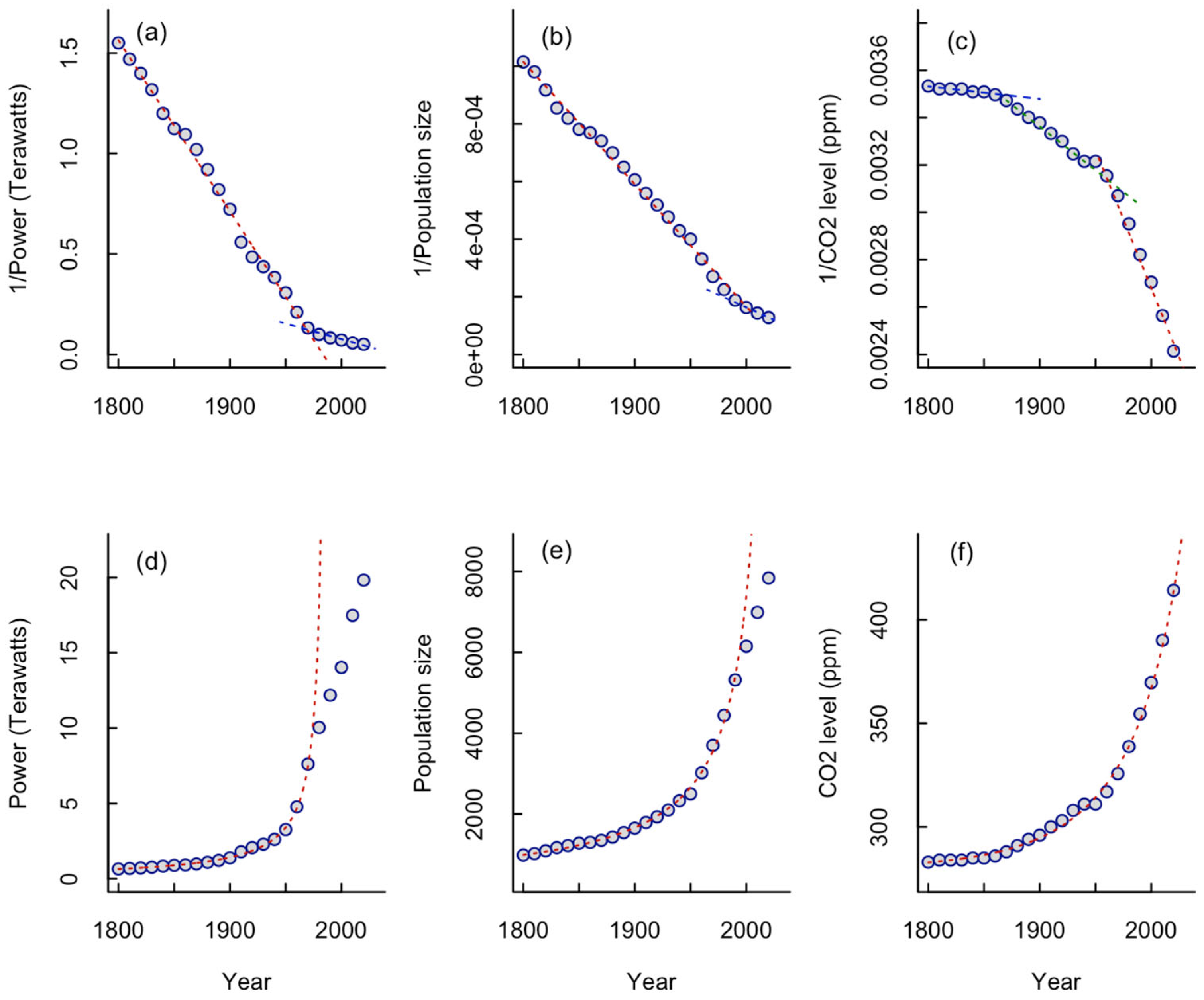
Figure 1a–f depicts the overall inverse and total trajectories of global power, population size, and atmospheric CO₂ levels. If the negative straight line in the inverse plots remains unchanged, then there is no change in the mechanism of growth. For example, the inverse power plot (1/Pw) showed a negative linear slope between 1800 and 1970 (y = 16.90 − 0.00852x; F_1,16 = 3358; p = 2.2 × 10⁻¹⁶; R² = 0.995), and an important decreasing trend in growth rates from 1980 and 2020 (y = 2.536 − 0.00123x; F_1,3 = 152.6; p = 0.00114; R² = 0.974) (Figure 1a). The power growth rate decreased by a factor of 6.9 between these two periods. The inverse population size plot (1/N) showed a negative linear slope, indicating a hyperbolic growth rate from 1800 to 1990 (y = 8.658 × 10⁻³−4.246 × 10⁻⁶x; F_1,18 = 3210; p = 2.2 × 10⁻¹⁶; R² = 0.994), for the period 2000–2020, the population growth rate decreased by a factor of 2.4 (y = 3.667 × 10⁻³ − 1.752 × 10⁻⁶x; F_1,1 = 227; p = 0.042; R² = 0.991) (Figure 1b). In contrast, the inverse CO₂ plot (1/CO₂) showed changes toward a faster hyperbolic trajectory, indicated by the observed downward bending trend (Figure 1c). The first sequence between 1800 and 1860 showed a weak negative slope (y = 4.485 × 10⁻³ − 5.295 × 10⁻⁷x; F_1,5 = 45.15; p = 0.0011; R² = 0.880), an increasing growth rate between 1870 and 1940 (y = 1.036 × 10⁻² − 3.683 × 10⁻⁶x; F_1,6 = 974.4; p = 7.18 × 10⁻⁸; R² = 0.993). The growth rate of the atmospheric CO₂ concentrations during the period 1870–1940 was 6.96 times higher than during the period 1800–1860 (Figure 1c). From 1950 to 2020, the growth rate of the atmospheric CO₂ even increased further, by a factor of three (y = 2.600 × 10⁻² − 1.166 × 10⁻⁵x; F_1,6 = 468; p = 6.37 × 10⁻⁷; R² = 0.985). In fact, during the last seventy years, the atmospheric CO₂ growth rates increased by a factor of twenty-two compared with the period 1800–1860.

In Figure 1d, we find that power data Pw_(t) from 1800 to 1970 can be well fitted using a hyperbolic model (red broken line) with parameters T = 1384 years, c = 0.092 Terawatts, and the singularity year t_l = 1987,

$$E_{\left(t\right)}={\displaystyle \frac{C}{e^{\left(t_l-t\right)/T}-1}}.$$

(8)

In Figure 1e, we find that population size data N_(t) from 1800 to 1990 can be well fitted using a hyperbolic model (red broken line) with parameters T = −768.3 years, c = −253 million people, and the singularity year t_l = 2026.7,

$$N_{\left(t\right)}={\displaystyle \frac{C}{e^{\left(t_l-t\right)/T}-1}}.$$

(9)

Finally, in Figure 1f, we find that atmospheric CO₂ concentration data CO_2(t) from 1800 to 2020 can be well fitted using a hyperbolic model (red broken line) with parameters T = −64.6 years, c = −279.8 ppm, and the singularity year t_l = 2092.3.

$${CO}_{2\left(t\right)}={\displaystyle \frac{C}{e^{\left(t_l-t\right)/T}-1}}.$$

(10)

3.2. Coupled Dynamics of the Energy Conversion, Human Population, and Atmospheric CO₂

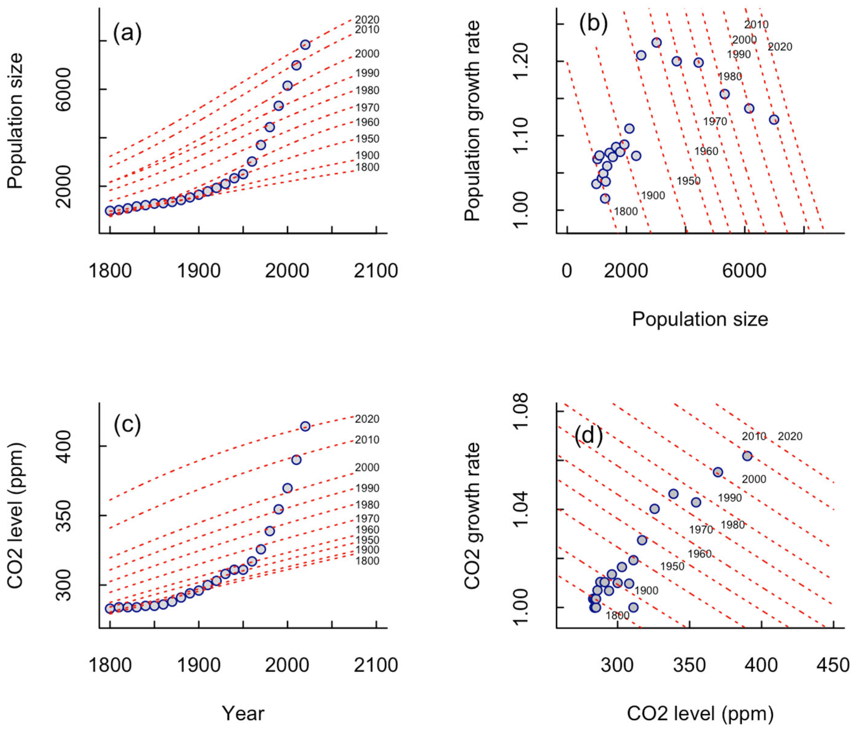
The self-acceleration process exhibited by the global population size (N) and the atmospheric CO₂ concentration (CO₂) can be represented by the phenomenon of “relaying” [21], the two system variables (N and CO₂) are expanding according to a series of overlapped self-limiting (logistic) curves whose parameters (c and T) can be influenced by the global power use (y_t) and power growth rates (R_y,t) (Figure 2). A model for the temporal pattern of population growth rates that includes the positive effect of global power (y_t) on parameter c and the negative effect of power growth rate (R_y,t) on parameter T was the best model according to AICc values, Akaike’s weights and the root-mean-squared-error (rsme) estimates (model 5;

Table 1. Logistic models for human population and atmospheric CO₂ dynamics and the effects of global power and power decadal growth rate (Equation (3)). Parameter values are given in the table’s columns and the standard error in parentheses. The model notations are as follows: c is the carrying capacity for the population size and atmospheric CO₂; t_l is the time at which x(t_l) = c/2; and T is the growth time in years. α, β and γ represent the effects of the power (y_t) and power growth rates (R_y,t) on the parameters c and T. AIC_c indicates the Akaike information criterion corrected for the small sample size; w_i is Akaike’s weights; rsme is the root-mean-square error. The model with the highest support is highlighted in boldface.

Population Models	c	tl	T	α	β	γ	AICc	$∆$AICc	wi	rsme	n	p
$1. x_{\left(t\right)}={\displaystyle \frac{(c+\alpha ·y_t)}{e^{\left(t_l-t\right)/\left(T\right)}+1}}$	2799.9 (1019.6)	1900 (84)	124.1 (28.9)	410.4 (87.4)	---	---	275.8	7.2	0	99.9	23	5
$2. x_{\left(t\right)}={\displaystyle \frac{\left(c\right)}{e^{\left(t_l-t\right)/(T+\beta ·y_t)}+1}}$	58,476.0 (6934)	2670 (51.9)	208.6 (14.9)	---	7.10 (1.2)	---	344.1	75.4	0	1876.8	23	5
$3. x_{\left(t\right)}={\displaystyle \frac{\left(c\right)}{e^{\left(t_l-t\right)/(T+\gamma ·R_{y,t})}+1}}$	5.96 × 105 (1.12 × 107)	2371 (1585)	83.0 (4.45)	---	---	−13.10 (48)	336.3	67.7	0	313.6	23	5
$4. x_{\left(t\right)}={\displaystyle \frac{(c+\alpha ·y_t)}{e^{\left(t_l-t\right)/(T+\beta ·y_t)}+1}}$	4.8 × 104 (2.0 × 106)	2701 (1.0 × 104)	227.1 (225)	7801 (3.2 × 105)	−0.75 (10.2)	---	271.4	2.8	0.20	712.0	23	6
$\mathbf{5}\mathbf{.} {\mathit{x}}_{\left(\mathit{t}\right)}={\displaystyle \frac{(\mathit{c}+\mathit{\alpha }·{\mathit{y}}_{\mathit{t}})}{{\mathit{e}}^{\left({\mathit{t}}_{\mathit{l}}-\mathit{t}\right)/(\mathit{T}+\mathit{\gamma }·{\mathit{R}}_{\mathit{y},\mathit{t}})}+\mathbf{1}}}$	3405.2 (323.1)	1947.1 (14.4)	150.1 (9.99)	458.7 (13.3)	---	−153.1 (49.3)	268.7	0.00	0.78	76.3	23	6
$6. x_{\left(t\right)}={\displaystyle \frac{\left(c\right)}{e^{\left(t_l-t\right)/(T+\beta ·y_t+\gamma ·R_{y,t})}+1}}$	7836.8 (600.6)	1974.5 (4.5)	78.6 (4.72)	---	−3.04 (0.48)	−80.9 (16.6)	335.4	66.7	0	1673.5	23	6
Atmospheric CO2 models	c	tl	T	α	β	γ	AICc	$∆$AICc	wi	rsme	n	p
$7. x_{\left(t\right)}={\displaystyle \frac{(c+\alpha ·y_t)}{e^{\left(t_l-t\right)/(T+\gamma ·R_{y,t})}+1}}$	576.5 (5.3)	1882.04 (25.6)	521.1 (360.4)	9.9 (0.8)	---	2213.9 (4960.3)	122.2	3.4	0.12	4.9	23	6
$8. x_{\left(t\right)}={\displaystyle \frac{(c+\alpha ·y_t)}{e^{\left(t_l-t\right)/(T+\beta ·y_t)}+1}}$	534.3 (156.7)	1725.8 (515.2)	895.8 (397)	3.57 (6.0)	−26 (17.6)	---	121.7	2.9	0.14	12.0	23	6
$9. x_{\left(t\right)}={\displaystyle \frac{\left(c\right)}{e^{\left(t_l-t\right)/(T+\gamma ·R_{y,t})}+1}}$	5190.5 (73,331)	3303.1 (8979.8)	516.9 (440.5)	---	---	−71.4 (349.5)	192.3	73.5	0.0	14.5	23	5
$\mathbf{10}\mathbf{.} {\mathit{x}}_{\left(\mathit{t}\right)}={\displaystyle \frac{\left(\mathit{c}\right)}{{\mathit{e}}^{\left({\mathit{t}}_{\mathit{l}}-\mathit{t}\right)/(\mathit{T}+\mathit{\beta }·{\mathit{y}}_{\mathit{t}})}+\mathbf{1}}}$	452.0 (15.23)	1493.1 (66.3)	654.0 (45.8)	---	−21.8 (1.9)	---	118.8	0.0	0.63	3.05	23	5
$11. x_{\left(t\right)}={\displaystyle \frac{\left(c\right)}{e^{\left(t_l-t\right)/(T+\beta ·y_t+\gamma ·R_{y,t})}+1}}$	453.9.0 (16.5)	1484.5 (75.3)	686.4 (82.3)	---	−22.9 (3.1)	−29.9 (60.02)	122.2	3.4	0.12	3.11	23	6

). Global power expands human population carrying capacity, while high power growth rates shorten the growth time parameter, thereby increasing the population growth rate. This model is supported by the cumulative w_i, indicating a high summed probability (78%) that it is the best model compared with the competing models. This can be interpreted as follows: the expansion of the human population was driven by two forces: the continuous long-term increase in power and faster interdecadal changes in power growth rates, which shifted the temporal pattern of population growth as a series of self-limiting (S-shaped) curves that overlap [21] (Figure 2a; Table 1).

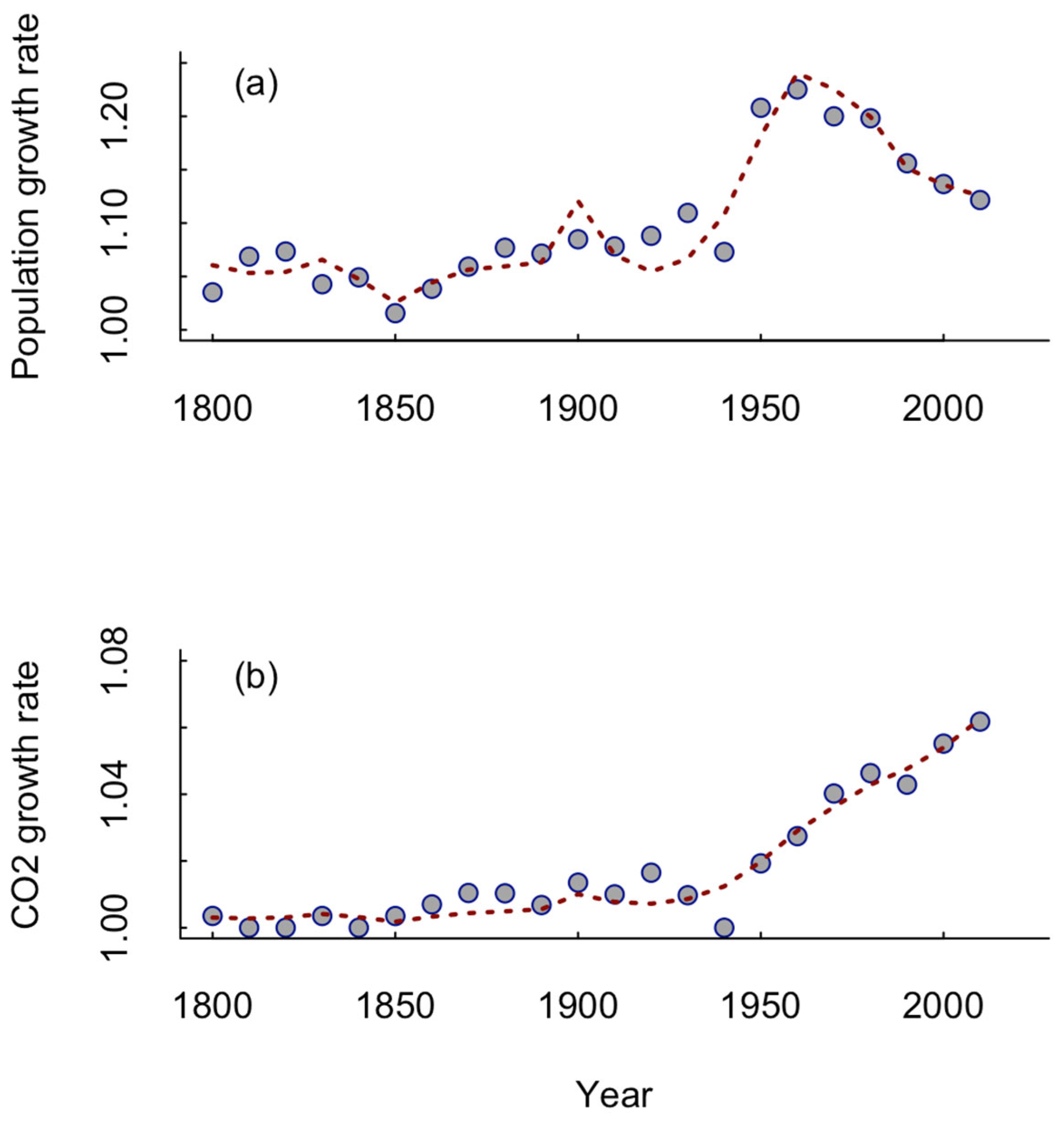
I transformed the time-plot representation of Figure 2a into the r_t–x_t growth rate curve versus population size (Figure 2b). The resultant plot provides details of human global population changes during the last 220 years that are not visible in the time-plot representation (Figure 2a). First, the net rate of change of the global population over these two centuries showed a humped-like shape, suggesting a period of hyperbolic growth (positive feedback) and a posterior negative feedback process (Figure 2a). A population dynamic model for growth rates (Equation (6)), including global power consumption (y_t) and power growth rate (R_y,t) as positive effects on r_m, was the best model according to AICc values, Akaike’s weights, root-mean-squared-error (RMSE) and the coefficient of prediction (model 4;

Table 2. Dynamic models for human population and atmospheric CO₂ growth rates influenced by global power and power decadal growth rate (Equation (6)). Parameter values are given in the table’s columns and the standard error in parentheses. The model notations are as follows: r_m is the maximum net growth rate, and c is the intensity of negative feedback. α, β and γ represent the effects of the power (y_t) and power growth rates (R_y,t) on the parameters r_m and c; AIC_c indicates the Akaike information criterion corrected for the small sample size; w_i is Akaike’s weight; rsme is the root-mean-square error. The model with the highest support is highlighted in boldface.

Population Dynamic Growth Models	rm	c	α	β	γ	AICc	$∆$AICc	wi	rsme	σ2
$1. r_t=r_m·e^{\left[-(c+\alpha ·y_t)·x_t\right]}$	0.94 (0.002)	−9.1 × 10−5 (1.3 × 10−5)	4.0 × 10−6 (7.2 × 10−7)	---	---	−82.0	17.4	0.0	0.04	0.49
$2. r_t=(r_m+\beta ·y_t)·e^{\left[-c·x_t\right]}$	0.92 (0.02)	−0.00013	---	−0.03 (0.002)	---	−74.2	25.2	0.0	0.05	−0.25
$3. r_t=(r_m+\gamma ·r_{y,t})·e^{\left[-c·x_t\right]}$	1.01 (1.2 × 10−2)	−1.2 × 10−5 (3.4 × 10−6)	---	---	0.37 (0.06)	−86.7	12.6	0.0	0.03	0.77
$\mathbf{4}\mathbf{.}{\mathit{r}}_{\mathit{t}}=({\mathit{r}}_{\mathit{m}}+\mathit{\beta }·{\mathit{y}}_{\mathit{t}}+\mathit{\gamma }·{\mathit{r}}_{\mathit{y},\mathit{t}})·{\mathit{e}}^{\left[-\mathit{c}·{\mathit{x}}_{\mathit{t}}\right]}$	1.11 (0.015)	0.0001 (1.8 × 10−5)	---	0.09 (0.02)	0.56 (0.06)	−99.4	0.0	0.63	0.02	0.89
$5. r_t=(r_m+\beta ·y_t)·e^{\left[-(c+\alpha ·y_t)·x_t\right]}$	0.98 (0.04)	−4.7 × 10−5 (3.9 × 10−5)	4.4 × 10−6 (7.2 × 10−7)	0.02 (0.018)	---	−80.3	19.1	0.0	0.04	0.68
$6. r_t=(r_m+\beta ·y_t+\gamma ·r_{y,t})·e^{\left[-(c+\alpha ·y_t)·x_t\right]}$	1.07 (0.03)	7.0 × 10−5 (3.7 × 10−5)	1.4 × 10−6 (8.3 × 10−7)	0.06 (0.02)	0.42 (0.10)	−98.3	1.1	0.37	0.02	0.90
Atmospheric CO2 growth models	rm	c	α	β	γ	AICc	$∆$AICc	wi	rsme	σ2
$7. r_t=r_m·e^{\left[-(c+\alpha ·y_t)·x_t\right]}$	0.93 (0.06)	−2.6 × 10−4 (2.4 × 10−4)	−5.4 × 10−6 (3.8 × 10−6)	---	---	−153.0	11.1	0.003	0.007	0.92
$8. r_t=(r_m+\beta ·y_t)·e^{\left[-c·x_t\right]}$	1.02 (0.07)	6.3 × 10−5 (2.4 × 10−4)	---	4.2 × 10−3 (1.8 × 10−3)	---	−158.0	6.1	0.03	0.006	0.93
$9. r_t=(r_m+\gamma ·r_{y,t})·e^{\left[-c·x_t\right]}$	0.85 (0.01)	−5.7 × 10−4 (4.8 × 10−5)	---	---	0.012 (0.012)	−152.1	12.0	0.002	0.007	0.85
$\mathbf{10}\mathbf{.} {\mathit{r}}_{\mathit{t}}=({\mathit{r}}_{\mathit{m}}+\mathit{\beta }·{\mathit{y}}_{\mathit{t}}+\mathit{\gamma }·{\mathit{r}}_{\mathit{y},\mathit{t}})·{\mathit{e}}^{\left[-\mathit{c}·{\mathit{x}}_{\mathit{t}}\right]}$	1.11 (0.07)	0.0004 (0.0002)	---	0.007 (0.002)	0.04 (0.01)	−163.6	0.0	0.67	0.005	0.94
$11. r_t=(r_m+\beta ·y_t)·e^{\left[-(c+\alpha ·y_t)·x_t\right]}$	1.02 (6.1 × 10−2)	5.4 × 10−5 (2.1 × 10−4)	1.5 × 10−5 (5.4 × 10−6)	1.04 × 10−2 (3.0 × 10−3)	---	−161.0	3.1	0.14	0.006	−0.79
$12. r_t=(r_m+\beta ·y_t+\gamma ·r_{y,t})·e^{\left[-(c+\alpha ·y_t)·x_t\right]}$	1.08 (0.073)	2.9 × 10−4 (2.4 × 10−4)	6.1 × 10−6 (7.3 × 10−6)	8.6 × 10−3 (3.2 × 10−3)	0.03 (0.017)	−161.0	3.0	0.15	0.006	0.95

; Figure 3a). This model is supported by the cumulative wi, indicating that it has a high summed probability (63%) of being the best model, and a very good coefficient of prediction (Table 2).

The best model for the temporal pattern of atmospheric CO₂ concentration includes global power (y_t) as a negative effect on parameter T, the growth time in years (model 10; Table 1). The expansion of global power decreases the growth time, which in turn increases the CO₂ growth rate. This model is supported by the cumulative w_i, indicating a high summed probability (63%) of being the best model compared with the competing model. This can be interpreted as follows: the increase in entropy production in the atmosphere (CO₂ concentration) is mainly driven by one force, the continuous long-term increase in global energy consumption, influencing the growth rate of the CO₂ concentration (Figure 2c; Table 1). This can explain the acceleration in atmospheric CO₂ concentration over the last decades, while population growth, by contrast, is decelerating (Figure 2b,d).

The time-plot representation of Figure 2c, in the r_t–x_t CO₂ growth rate curve versus atmospheric CO₂ levels (Figure 2d), provides details of atmospheric CO₂ growth rates that are not visible in the time-plot representation (Figure 2c). The net rate of change of the atmospheric CO₂ levels showed a positive trend, indicating a growth (positive feedback) (Figure 2d). The best dynamic model for CO₂ growth rates (Equation (6)), including global power (y_t) and power growth rate (R_y,t) as positive effects on r_m, according to AICc values, Akaike’s weights, root-mean-squared-error (RMSE) and the coefficient of prediction (model 10; Table 2; Figure 3b). This model is supported by the cumulative wi, indicating that it has a high summed probability (67%) of being the best model, compared with the other competing models.

Total trajectory predictions from the models of population and atmospheric CO₂ growth rates, which include the continuous long-term increase in global power and the faster interdecadal changes in energy growth rates on parameter r_m, showed very high coefficients of prediction (Table 2), indicating that these simple models were able to capture the long- and short-term fluctuations of human population and CO₂ growth rates (Figure 3). This can be interpreted as follows: the continuous long-term increase in energy availability and the faster interdecadal changes in energy growth rates, shifting the population and CO₂ growth rate curve upwards along the Y-axis (Figure 2b,d; a vertical perturbation effect [33]). The comparison between models indicates that while population growth rate is more strongly influenced by power growth rate (R_y,t), atmospheric CO₂ growth rates are mainly driven by global power (y_t) (Table 2).

4. Discussion

The expansion of power use has played a central role in fueling the positive feedback loop of human population and CO₂ dynamics over the past two centuries [7,15,43]. The expansive dynamics of our global society over the last 220 years are driven by changes in total global power (energy consumption/time) use and its growth rate, which, in turn, influence population dynamics. The intertwined dynamics of power, population, and atmospheric CO₂ growth rates are characterized by different periods of acceleration and stagnation. While power use and population dynamics showed a first period (1800–1970) of accelerated growth and stagnation since 1980, atmospheric CO₂ concentration dynamics are characterized by hyperbolic growth over the period studied (1800–2020).

Our current population growth rates appear to be supported by energy influxes during the first decades after 1950 [44]. The oil and natural gas era transformed social, political, and economic relations from those of the coal age [45]. After 1940, a new energy era emerged, characterized by accelerated population and economic growth and increased human environmental impacts worldwide, the “Great Acceleration” [26]. During this period, there was a shift towards reliance on oil and natural gas [12,44], which caused significant upheaval in power use, population, and the economy after 1940–50. In the oil era, the growth rate of power tripled, leading to unprecedented levels of material production, population growth, and environmental degradation [26].

The results showed that from 1970 onward, the dynamics of growth rates in power and population were characterized by diminishing returns [7,8,15,46]. Since 1970, power growth rates have decreased by a factor of seven, while population growth rates started to decrease a decade later by a factor of two and a half. The positive feedback loop between power and population is leading our civilization into a new era of stagnation [8,47]. This trend is closely associated with the observation that the energy return on investment (EROI) of the most important energy sources, such as oil and natural gas, has generally declined over the past fifty years [3,12,47,48]. The results of this study showed that the past increases in power consumption and population size are entering an era of diminishing returns [15]. A major potential problem is that the growth rate of power is trending downward faster than the population growth rate since 1970. We are living in an era of stagnation in the per capita power growth rate.

The population dynamic models showed that global power (y_t) and its growth rate (R_y,t) are forcing factors diminishing the growth time in years (T from Equation (3)) and increasing the (mean) potential growth rate (r_m from Equation (6)). They increase the human population growth rate. The explosive human expansion since the beginning of the 19th century would result from two forces acting on a single population parameter: the human population growth rate. These two forces, power use and the growth rate, propelled our expansive intrinsic population dynamic system. Access to high-energy reserves (oil and natural gas) increased human civilization’s energy power and turnover rates [47]. So, the human population was involved in a disequilibrium expansive dynamic able to grow and, at the same time, exploit new reserves of raw materials and energy, creating more people, more technology, and new lifestyles that require more energy consumption, closing the loop back by adding more people [8,9,49,50].

The new energetic environment, in which our primary energy source (oil) was accumulated underground, enabled the observed population trend of accelerated, continuous growth. In the fitted population models, the power growth rate (R_y,t) is the main force influencing the parameters T and r_m. This can be interpreted as a high-power growth rate increasing the reproductive rate and life expectancy in the global population system. This effect on the population growth rate is consistent with the maximum power principle, since the growth rate in power between decades reflects the capacity of the human population to convert that energy flow into physical population growth [4,5,30].

On the other hand, the effect of global power (y_t) on the parameters (T and r_m) can be interpreted as a gradual, continuous force that improves our lifestyles and consumption. As an analogy to Alfred J. Lotka’s [30] wheel, global power use was “enlarging the wheel,” while the power growth rate was causing it to “spin faster.” Our expansionary population dynamic is starting to reach its limits. Population size and power are engaged in a positive feedback loop that explains the dynamics of our population and economic system [44], making our present human societies increasingly vulnerable to collapse [15].

The best model for the temporal pattern of atmospheric CO₂ concentration is mainly driven by one force: global power (y_t), influencing the growth time in years (T) in Equation (3) and the net (mean) potential growth rate (r_m) in Equation (6). Suggesting that global power use is the driving factor in the dynamics of atmospheric CO₂ concentration. In sum, the atmospheric CO₂ dynamics are driven by the current size of our socioeconomic system, and the distant past upward trend will influence the future trend in atmospheric CO₂ levels [29].

This finding raises the possibility that the climate system could exceed critical thresholds [26], even if we can reduce fossil fuel use in the following decades. It seems that we are trapped between a rock and a hard place. Without a drastic switch to renewable energy sources and a reduction of our civilization’s wealth and size, atmospheric carbon dioxide concentrations will continue to rise. In the nonequilibrium system of our industrial civilization, heat, particles, and CO₂ emitted by humans, heat engines, machines, reactors, cars, and planes alter the atmosphere’s chemical composition. The rate of this change is proportional to the total size of our population and power use [17,51].

Our global society appears to be facing a key contradiction, with no obvious way out. If we do not reduce the size of our global society and power use in the coming decades, CO₂ levels and temperature increases will exceed habitable limits in many parts of the planet. The end road, it seems to be a radical simplification and reduction of our material production system and population size [50,51]. It seems that only by collapsing the size of our global population and energy consumption system, by shrinking and slowing Lotka’s wheel [29], can our resource demands and waste production decline [52].

The transition to renewable energy sources in the future is likely to result in a significant decrease in per capita net energy availability over the coming decades [53,54,55,56,57] because solar and wind energy sources have lower EROI levels than fossil fuels [12,45,58]. The energy return on investment (EROI) levels of renewable energy sources are significantly lower than the thresholds identified in the literature as required to sustain the high-power use levels and wealth of current industrial complex societies. A major challenge for humanity will be generating sizeable new energy investments while the power growth rate is declining [3,4,12]. While renewable energy is often seen as the solution for creating sustainable societies, it presents new challenges that are not widely discussed. A common belief is that technological advancements alone can decarbonize our energy systems; however, the total entropy export costs of renewable energy production may shift ecological problems rather than resolve them [10]. Therefore, the results of this study suggest that the dynamics of this highly interdependent system, population, power, and atmospheric CO₂ could constrain the potential for general sustainable development goals and shared socioeconomic pathways (SSPs) [7].

Over the past 60 years, the growth rate of energy has mirrored that of the first three decades of the 20th century, albeit with a population that is four times larger. Many countries are now encountering the constraints on growth outlined in “The Limits to Growth” [59]. Today, many people are still transitioning from agrarian to industrial lifestyles [60,61]. The slowing power growth rates could result in periods of heightened sociopolitical instability and violence. Historically, major energy transitions have often been associated with increased levels of violence and social unrest [62,63]. In the coming decades, we are likely to witness slow growth in energy consumption while the global population exceeds eight billion. Additionally, there has been a rise in signs of political instability, riots, civil unrest, and armed conflicts in recent years [64,65,66]. Today, the global human population-economic system is a giant 20 tera-watt primary power machine. Putting this number in terms of primary-power “laborers”, on average, each of the 8 billion living humans is served by ~32 primary-power “slaves”. Global humanity today is functioning as a 260 billion person-equivalent mega-population [67].

5. Conclusions

We are entering a new era characterized by a declining power growth rate that outpaces the decline in global population growth, while the growth rate of atmospheric CO₂ is accelerating. This complex nexus will fundamentally alter our social, economic, and political structures, as well as the global climate.

The shift to renewable energy is reversing the agrarian-to-industrial transition of the last two centuries [60]. This change is already evident in social and energy-related shifts [68,69]. Depleting fossil fuels slows global power growth and causes greater inequality, civil unrest, and stress on health and social security. We also face climate change, the sixth mass extinction, soil erosion, and reduced ecosystem services [70]. Moving to sustainability is urgent, as the industrial age will be shorter than previous regimes [71].

The use of simple dynamic models may limit this study because they do not account for the complexities and variations in population density, energy consumption patterns, fertility rates, urbanization, education, technology, and economic growth across different societies worldwide. However, I would like to shift the perspective by noting that in this article, I do not assume that all these variables must be included. Moreover, their exclusion does not inherently diminish the model’s ability to explain the observed phenomena. Contrary to being a limitation, there is a conceptual rationale for preferring simple models [33]. Evidence suggests that systems characterized by general micro-level complexity can be effectively described by simple models with only a few variables [34,35]. Therefore, it appears that the global population is growing as a unified dynamic system, with its size reflecting the aggregate of all economic, social, and cultural activities [22].

As we focus on the biophysical limitations of a finite world [72], the future will depend on how we organize, manage, and distribute energy and power, influencing the potential for sustainable and equitable communities [45].

References

1. Kallis, G. Radical dematerialization and degrowth. Philos. Trans. R. Soc. A Math. Phys. Eng. Sci. 2017, 375, 20160383. [Google Scholar] [CrossRef] [PubMed]
2. Krall, L.; Gowdy, J. Dialectical and Evolutionary Materialism: Expanding methodological pluralism in ecological economics. Ecol. Econ. 2025, 230, 108487. [Google Scholar] [CrossRef]
3. Hall, C.A.S.; Klitgaard, K. (Eds.) Biophysical economics: The economics perspective. In Energy and the Wealth of Nations: An Introduction to Biophysical Economics; Springer International Publishing: Berlin/Heidelberg, Germany, 2018; pp. 101–120. [Google Scholar]
4. Hall, C.A.S.; McWhirter, T. Maximum power in evolution, ecology and economics. Philos. Trans. R. Soc. A Math. Phys. Eng. Sci. 2023, 381, 20220290. [Google Scholar] [CrossRef] [PubMed]
5. Vermeij, G. The Evolution of Power: A New Understanding of the History of Life; Princeton University Press: Princeton, NJ, USA, 2023. [Google Scholar]
6. Herrmann-Pillath, C. Constitutive Explanations as a Methodological Framework for Integrating Thermodynamics and Economics. Entropy 2016, 18, 18. [Google Scholar] [CrossRef]
7. Lima, M. The link between human population dynamics and energy consumption during the Anthropocene. Anthr. Rev. 2025, 12, 3–17. [Google Scholar] [CrossRef]
8. Lima, M.; Berryman, A.A. Positive and negative feedbacks in human population dynamics: Future equilibrium or collapse? Oikos 2011, 120, 1301–1310. [Google Scholar] [CrossRef]
9. Snyder, B.F. The genetic and cultural evolution of unsustainability. Sustain. Sci. 2020, 15, 1087–1099. [Google Scholar] [CrossRef] [PubMed]
10. Wessling, B. What a Coincidence! On Unpredictability, Complexity and the Nature of Time; Springer Nature: Wiesbaden, Germany, 2023. [Google Scholar]
11. Ellis, E.C. Ecology in an anthropogenic biosphere. Ecol. Monogr. 2015, 85, 287–331. [Google Scholar] [CrossRef]
12. Hall, C.A.S. The history, future, and implications of EROI for society. In Energy Return on Investment: A Unifying Principle for Biology, Economics, and Sustainability; Springer: New York, NY, USA, 2017; p. 174. [Google Scholar]
13. Smil, V. Energy and Civilization: A History; MIT Press: Cambridge, UK, 2017; p. 535. [Google Scholar]
14. Johansen, A.; Sornette, D. Finite-time singularity in the dynamics of the world population, economic and financial indices. Phys. A Stat. Mech. Its Appl. 2001, 294, 465–502. [Google Scholar] [CrossRef]
15. Taylor, T.G.; Tainter, J.A. The nexus of population, energy, innovation, and complexity. Am. J. Econ. Sociol. 2016, 75, 1005–1043. [Google Scholar] [CrossRef]
16. Annila, A.; Salthe, S. Economies evolve by energy dispersal. Entropy 2009, 11, 606–633. [Google Scholar] [CrossRef]
17. Garrett, T.J. Are there basic physical constraints on future anthropogenic emissions of carbon dioxide? Clim. Change 2011, 104, 437–455. [Google Scholar] [CrossRef]
18. Herrmann-Pillath, C. Energy, growth, and evolution: Towards a naturalistic ontology of economics. Ecol. Econ. 2015, 119, 432–442. [Google Scholar] [CrossRef]
19. Cailleux, A. L’homme en surexpansion. Bull. Soc. Préhist. Fr. 1951, 48, 62–70. [Google Scholar] [CrossRef]
20. Van Von Foerster, H.; Mora, P.M.; Amiot, L.W. Doomsday: Friday, 13 November, AD 2026: At this date human population will approach infinity if it grows as it has grown in the last two millennia. Science 1960, 132, 1291. [Google Scholar] [CrossRef]
21. Meyer, F.; Vallee, J. The dynamics of long-term growth. Technol. Forecast. Soc. Change 1975, 7, 285–300. [Google Scholar] [CrossRef]
22. Kapitza, S.P. On the theory of global population growth. Phys. Uspekhi 2010, 53, 1287. [Google Scholar] [CrossRef]
23. Nielsen, R.W. Mechanism of hyperbolic growth explained. J. Econ. Libr. 2016, 3, 603–620. [Google Scholar]
24. Yakovenko, V.M. The end of hyperbolic growth in human population and CO2 emissions. Phys. A Stat. Mech. Its Appl. 2025, 661, 130412. [Google Scholar] [CrossRef]
25. Lima, M.; Gayo, E.M.; Estay, S.A.; Gurruchaga, A.; Robinson, E.; Freeman, J.; Latorre, C.; Bird, D. Positive feedbacks in deep-time transitions of human populations. Philos. Trans. R. Soc. B 2024, 379, 20220256. [Google Scholar] [CrossRef] [PubMed]
26. Steffen, W.; Broadgate, W.; Deutsch, L.; Gaffney, O.; Ludwig, C. The trajectory of the Anthropocene: The great acceleration. Anthr. Rev. 2015, 2, 81–98. [Google Scholar] [CrossRef]
27. Tainter, J.A. Energy, complexity, and sustainability: A historical perspective. Environ. Innov. Soc. Trans. 2011, 1, 89–95. [Google Scholar] [CrossRef]
28. Garrett, T.J. No way out? The double-bind in seeking global prosperity alongside mitigated climate change. Earth Syst. Dyn. 2012, 3, 1–17. [Google Scholar] [CrossRef]
29. Lotka, A.J. Contribution to the energetics of evolution. Proc. Natl. Acad. Sci. USA 1922, 8, 147–151. [Google Scholar] [CrossRef] [PubMed]
30. Odum, H.T.; Pinkerton, R.C. Time’s speed regulator: The optimum efficiency for maximum power output in physical and biological systems. Am. Sci. 1955, 43, 331–343. [Google Scholar]
31. Lineweaver, C.H. Beyond the Second Law: Darwinian evolution as a tendency for entropy production to increase. Entropy 2025, 27, 850. [Google Scholar] [CrossRef] [PubMed]
32. Herrmann-Pillath, C. Towards pragmatist thermodynamics: An essay on the natural philosophy of entropy and sustainability. Entropy 2025, 27, 1257. [Google Scholar] [CrossRef] [PubMed]
33. Royama, T. Analytical Population Dynamics; Springer Science & Business Media: Berlin, Germany, 1992. [Google Scholar]
34. Berryman, A.A. Principles of Population Dynamics and Their Application; Stanley Thornes: Cheltenham, UK, 1999. [Google Scholar]
35. Turchin, P. Complex Population Dynamics: A Theoretical/Empirical Synthesis; Princeton University Press: Princeton, NJ, USA, 2003. [Google Scholar]
36. Ritchie, H.; Rosado, P.; Roser, M. OurWorldinData.org. Energy. Available online: https://ourworldindata.org/energy (accessed on 24 May 2026).
37. Etheridge, D.M.; Steele, L.P.; Langenfelds, R.L.; Francey, R.J.; Barnola, J.M.; Morgan, V.I. Natural and anthropogenic changes in atmospheric CO2 over the last 1000 years from air in Antarctic ice and firn. J. Geophys. Res. Atmos. 1996, 101, 4115–4128. [Google Scholar] [CrossRef]
38. Cohen, J.E. Population growth and earth’s human carrying capacity. Science 1995, 269, 341–346. [Google Scholar] [CrossRef] [PubMed]
39. Verhulst, P. Notice sur la loi que la population suit dans son accroissement. Corresp. Math. Phys. 1838, 10, 113–129. [Google Scholar]
40. Burnham, K.P.; Anderson, D.R. Model Selection and Multimodel Inference: A Practical Information Theoretic Approach; Springer Science and Business Media: New York, NU, USA, 2002; p. 485. [Google Scholar]
41. Kvalseth, T.O. Note on the R2 measure of goodness of fit for nonlinear models. Bull. Psychon. Soc. 1983, 21, 79–80. [Google Scholar] [CrossRef]
42. Turchin, P.; Currie, T.E.; Whitehouse, H.; François, P.; Feeney, K.; Mullins, D.; Hoyer, D.; Collins, C.; Grohmann, S.; Savage, P.; et al. Quantitative historical analysis uncovers a single dimension of complexity that structures global variation in human social organization. Proc. Natl. Acad. Sci. USA 2018, 115, E144–E151. [Google Scholar] [CrossRef] [PubMed]
43. Krall, L. Bitter Harvest: An Inquiry into the War between Economy and Earth; State University New York Press: Albany, NY, USA, 2022; p. 182. [Google Scholar]
44. Garrett, T.J. Long-run evolution of the global economy: 1. Physical basis. Earth’s Future 2014, 2, 127–151. [Google Scholar] [CrossRef]
45. Mitchell, T. Carbon democracy. Econ. Soc. 2009, 38, 399–432. [Google Scholar] [CrossRef]
46. Fisher-Kowalski, M.; Krausmann, F.; Pallua, I. A socio-metabolic reading of the Anthropocene. Anthr. Rev. 2014, 1, 8–33. [Google Scholar] [CrossRef]
47. Hall, C.A.; Lambert, J.G.; Balogh, S.B. EROI of different fuels and the implications for society. Energy Policy 2014, 64, 141–152. [Google Scholar] [CrossRef]
48. Bonaiuti, M. Are we entering the age of involuntary degrowth? Promethean technologies and declining returns of innovation. J. Clean. Prod. 2018, 197, 1800–1809. [Google Scholar] [CrossRef]
49. Laherrère, J.; Hall, C.A.; Bentley, R. How much oil remains for the world to produce? Comparing assessment methods and separating fact from fiction. Curr. Res. Environ. Sustain. 2022, 4, 100174. [Google Scholar] [CrossRef]
50. Sibani, P.; Rasmussen, S. Human wealth evolution: Trends and fluctuations. Phys. A Stat. Mech. Its Appl. 2020, 558, 124985. [Google Scholar] [CrossRef]
51. Garrett, T.J. Long-run evolution of the global economy–Part 2: Hindcasts of innovation and growth. Earth Syst. Dyn. 2015, 6, 673–688. [Google Scholar] [CrossRef]
52. Odum, H.T.; Odum, E.C. The prosperous way down. Energy 2006, 31, 21–32. [Google Scholar] [CrossRef]
53. Hagens, N.J. Economics for the future–Beyond the superorganism. Ecol. Econ. 2020, 169, 106520. [Google Scholar] [CrossRef]
54. Garrett, T.J.; Grasselli, M.; Keen, S. Lotka’s wheel and the long arm of history: How does the distant past determine today’s global rate of energy consumption? Earth Syst. Dyn. 2022, 13, 1021–1028. [Google Scholar] [CrossRef]
55. King, L.C.; Van Den Bergh, J.C. Implications of net energy-return-on-investment for a low-carbon energy transition. Nat. Energy 2018, 3, 334–340. [Google Scholar] [CrossRef]
56. Capellán-Pérez, I.; De Castro, C.; González, L.J.M. Dynamic Energy Return on Energy Investment (EROI) and material requirements in scenarios of the global transition to renewable energies. Energy Strat. Rev. 2019, 26, 100399. [Google Scholar] [CrossRef]
57. Dupont, E.; Koppelaar, R.; Jeanmart, H. Global available solar energy under physical and energy return on investment constraints. Appl. Energy 2020, 257, 113968. [Google Scholar] [CrossRef]
58. de Castro, C.; Capellán-Pérez, I. Standard, point of use, and extended energy return on energy invested (EROI) from comprehensive material requirements of present global wind, solar, and hydro power technologies. Energies 2020, 13, 3036. [Google Scholar] [CrossRef]
59. Meadows, D.H.; Meadows, D.L.; Randers, J.; Behrens, W.W., III. The Limits to Growth: A Report to the Club of Rome’s Project on the Predicament of Mankind; Universe Books: New York, NY, USA, 1972. [Google Scholar]
60. Fisher-Kowalski, M.; Haberl, H. Socioecological Transitions and Global Change: Trajectories of Social Metabolism and Land Use; Klagenfurt University: Vienna, Austria, 2007. [Google Scholar]
61. Krausmann, F.; Fischer-Kowalski, M.; Schandl, H.; Eisenmenger, N. The global sociometabolic transition: Past and present metabolic profiles and their future trajectories. J. Ind. Ecol. 2008, 12, 637–656. [Google Scholar] [CrossRef]
62. Fischer-Kowalski, M. Analyzing sustainability transitions as a shift between socio-metabolic regimes. Environ. Innov. Soc. Transit. 2011, 1, 152–159. [Google Scholar] [CrossRef] [PubMed]
63. Fischer-Kowalski, M.; Rovenskaya, E.; Krausmann, F.; Pallua, I.; Mc Neill, J.R. Energy transitions and social revolutions. Technol. Forecast. Soc. Change 2019, 138, 69–77. [Google Scholar] [CrossRef]
64. Turchin, P. End Times: Elites, Counter-Elites, and the Path of Political Disintegration; Penguin Press: New York, NY, USA, 2023; p. 352. [Google Scholar]
65. Ahmed, N.M. Failing States, Collapsing Systems: Biophysical Triggers of Political Violence; Springer Nature: Cham, Switzerland, 2017; p. 110. [Google Scholar]
66. Muñoz-Rodríguez, M.; Ferrero, R.; Luna, J.P.; Lima, M. Squeezed from the top: “Social Outburst” (2019) and elite overproduction. A study of the dynamics of Chilean political instability from the approach of Structural Demographic Theory. PLoS ONE 2024, 19, e0299063. [Google Scholar] [CrossRef] [PubMed]
67. Patzek, T.W. Thermal Power and Climate Change: A Data-Driven Analysis of Cause and Effect, 1800–2100. 2026. Available online: https://eartharxiv.org/repository/view/10865/ (accessed on 20 June 2026).
68. Sieferle, R.P. The Subterranean Forest: Energy Systems and the Industrial Revolution; White Horse Press: Winwick, UK, 2001. [Google Scholar]
69. Hall, C.A.S. The 50th anniversary of the limits to growth: Does it have relevance for today’s energy issues? Energies 2022, 15, 4953. [Google Scholar] [CrossRef]
70. Kemp, L.; Xu, C.; Depledge, J.; Ebi, K.L.; Gibbins, G.; Kohler, T.A.; Rockström, J.; Scheffer, M.; Schellnhuber, H.J.; Steffen, W.; et al. Climate Endgame: Exploring catastrophic climate change scenarios. Proc. Natl. Acad. Sci. USA 2022, 119, e2108146119. [Google Scholar] [CrossRef] [PubMed]
71. Soddy, F. Cartesian Economics: The Bearing of Physical Science Upon State Stewardship; Hendersons: London, UK, 1922. [Google Scholar]
72. Kümmel, R.; Lindenberger, D.; Paech, N. Energy, Entropy, Creativity: What Drives and Slows Economic Growth; Springer Nature: Berlin, Germany, 2025. [Google Scholar]
Figure 1. Inverse plots of (a) global power use (1/Pw), (b) global population size (1/N), and (c) atmospheric CO2 concentration (1/CO2) time series, revealing the different hyperbolic trajectories represented by decreasing (increasing) straight lines (red, blue, and green dotted lines; see text). Time series plot of (d) power use (Terawatts), (e) population size (million people), and (f) atmospheric CO2 concentration (ppm). Red broken lines are the fitted hyperbolic models (see text for details).
Sustainability 18 07179 g001
Figure 2. (a) Global time series of population size (gray dots) and the corresponding best-fit sigmoid curves (model 5, Table 1, red broken lines) based on the observed global power (yt) and power growth rate (Ry,t) values. (b) Transformation of (a) into a growth curve in the rt–xt format. The dotted red lines are the predicted curves for the best-fit dynamic model (model 4; Table 2). (c) Atmospheric CO2 concentration (gray dots) and the corresponding best-fit sigmoid curves (model 10; Table 1; red broken lines) based on the observed global power (yt) values. (d) Transformation of (c) into a growth curve in the rt–xt format. The dotted red lines are the predicted curves for the best-fit dynamic model (model 10; Table 2).
Sustainability 18 07179 g002
Figure 3. Comparison of the observed (a) human population and (b) atmospheric growth rates (gray circles) for the period 1800–2020, with predictions (red dotted line) from models 4 and 10, respectively (Table 2). Model validation and parameter values are in Table 2.
Sustainability 18 07179 g003