Article

Decision-Centric Portfolio Selection for Sustainable Supply Chain Risk Management: A Simulation-Optimization Framework for Robust Decision Support

1
Department of Management Engineering, Sangmyung University, Cheonan-si 31066, Chungcheongnam-do, Republic of Korea
2
Department of Business Information Systems and Operations Management, University of North Carolina at Charlotte, Charlotte, NC 28223, USA
*
Author to whom correspondence should be addressed.
Sustainability 2026, 18(13), 6863; https://doi.org/10.3390/su18136863
Submission received: 11 May 2026 / Revised: 28 June 2026 / Accepted: 1 July 2026 / Published: 6 July 2026
(This article belongs to the Section Sustainable Management)

Abstract

Sustainable supply chains are increasingly vulnerable to systemic risks, such as geopolitical conflicts at critical trade routes like the Strait of Hormuz or climate disasters, which reveal deep Environmental, Social, and Governance (ESG) weaknesses. Conventional optimization often fails in these “deep uncertainty” contexts, where reliable historical data are often scarce and qualitative factors are paramount. This study introduces a simulation-optimization framework that reframes risk management as a decision process rather than a purely computational one. Portfolios are parameterized across five key characteristics—prevention, vulnerability, resilience, recovery, and detection—to enable a genetic algorithm (GA) to generate a diverse ensemble of high-performing strategies. Instead of providing one “best” answer, the GA allows managers to evaluate multiple options against quantitative tail-risk measures and qualitative institutional factors. The framework produces a “trade-off map,” or Pareto frontier, visualizing the cost of protecting against downside risks. By adjusting the GA’s settings, decision makers can toggle between improving current plans and exploring new, structurally different strategies. The numerical results demonstrate that the GA consistently identifies high-performing portfolios, achieving at least 99.55% of the true optimal performance across all metrics while requiring only 25% of the computational evaluation budget of an exhaustive search space. Furthermore, the framework successfully generates a structurally diverse menu of near-optimal alternatives across all performance metrics, consistently outperforming Monte Carlo sampling in the quality of near-optimal solutions identified, particularly for tail-risk measures such as conditional value-at-risk. Ultimately, this approach integrates the manager’s professional judgment regarding non-quantifiable factors, such as political stability and social responsibility, with simulation data to support the selection of a robust, sustainable portfolio.

1. Introduction

Current supply chains operate in environments characterized by heightened uncertainty and systemic risk. Globalization, geopolitical tensions, climate-related disruptions, and pandemics have increased both the frequency and severity of supply chain disruptions. As a result, supply chain risk management (SCRM) has become a critical area of research and practice. Several approaches to managing supply chain risk have been proposed in the literature [1]. These approaches include optimization-based approaches [2] and simulation-based approaches. While these approaches provide valuable analytical insights, they often assume that decision-makers can rely on well-specified models and stable parameter estimates.
However, an increasing body of research argues that many real-world supply chain risks are better understood as “deep uncertainties,” where decision-makers face not only incomplete data but also ambiguity regarding model structure, parameter values, and even appropriate performance metrics [3,4]. In such contexts, the primary challenge is not merely computational but cognitive: managers must interpret uncertain and sometimes conflicting information while making strategic decisions under time pressure and organizational constraints. This shifts the focus of SCRM from identifying a single optimal solution to supporting effective decision-making under uncertainty.
Under such conditions, decision-makers are often better served by strategies that are robust, performing reasonably well across a wide range of scenarios, and adaptive, allowing for adjustment as new information becomes available [5]. Moreover, decision-makers differ in their attitudes toward risk and may prioritize different performance criteria, ranging from expected values to downside risk indicators such as Value at Risk (VaR) and Conditional Value at Risk (CVaR) [1]. Consequently, SCRM tools must accommodate heterogeneous risk preferences and facilitate the evaluation of trade-offs among competing objectives.
Simulation-based approaches are particularly well-suited to this setting because they can capture nonlinear, time-dependent interactions within supply chains [4]. However, their value lies not only in modeling complexity but also in their ability to generate multiple plausible scenarios and outcomes. Rather than seeking a single “best” solution, there is increasing recognition that decision support should focus on presenting a set of high-quality alternatives that reflect different assumptions, risk measures, and strategic priorities.
This paper introduces a decision-centric perspective on SCRM and presents a simulation-optimization framework designed to support managerial judgment under deep uncertainty. Specifically, a genetic algorithm (GA) is used not simply as a computational tool for efficiently searching large solution spaces, but as a mechanism for generating a diverse portfolio of high-performing SCRM strategies. These portfolios are parameterized across five key risk characteristics—prevention, vulnerability, resilience, recovery, and detection—allowing systematic exploration of trade-offs across multiple performance dimensions.
Importantly, the proposed framework is designed to produce a set of candidate solutions, rather than a single optimal portfolio. These solutions can be evaluated using multiple performance measures, including both mean-based metrics and downside risk measures such as CVaR, enabling decision-makers with different risk preferences to identify strategies aligned with their objectives. The resulting “trade-off map,” or Pareto frontier, provides a structured representation of the costs and benefits associated with different risk management strategies.
By reframing the role of optimization in SCRM, this study contributes to the literature in three ways. First, it shifts the focus from computational efficiency to decision support, arguing that the primary challenge in SCRM is cognitive rather than computational. Second, it demonstrates, to the best of the authors’ knowledge, for the first time in the SCRM portfolio context, how genetic algorithms can generate a diverse set of high-quality alternative portfolios rather than converging to a single solution, enabling managers with different risk attitudes to identify strategies aligned with their priorities. Third, it provides a multi-dimensional evaluation framework that formally accommodates risk preferences by presenting trade-offs across both mean-based performance measures and downside tail-risk indicators, enabling selection based on both quantitative metrics and qualitative organizational considerations.
Figure 1 illustrates the overall structure of the proposed decision-support framework. The left layer shows representative SCRM strategies that managers can invest in (e.g., finished goods inventory buffering, backup supplier contracts, early warning systems, and excess production capacity). The center layer shows the five portfolio parameters (p, q, r, s, y) that translate investment decisions into quantifiable effects on supply chain risk characteristics. The right layer shows the multi-dimensional performance dashboard (NetSCV, LTEV, VaR, CVaR) used to evaluate and compare portfolios. Arrows indicate that SCRM strategy choices are evaluated through the simulation-optimization engine, with the five-parameter layer serving as the structured interface between managerial decisions and quantitative analysis. The manager’s qualitative judgment enters at two points: in translating strategies into parameter investments, and in selecting among Pareto-optimal alternatives on the performance dashboard.

2. Literature Review

2.1. Supply Chain Risk Management

There is a rich and growing body of research on SCRM. A seminal review paper by Tang [6] provided an early, influential framework by categorizing risk mitigation strategies into four key areas: supply management, demand management, product management, and information management. Subsequent review papers, e.g., [1,7], structured the field, while recent analyses, e.g., [8,9] use bibliometric methods to map its evolution. The importance of the field was underscored by foundational empirical work such as [10,11], which demonstrated that supply chain disruptions have a significant negative effect on a firm’s operating performance and long-term stock price.
Heckmann, Comes and Nickel [1] discuss various definitions of supply chain risk, including “variation in the distribution of possible supply-chain outcomes, the likelihood, and its subjective values” [12] and “anything that disrupts or impedes the information, material, or product flows from origin and suppliers to the delivery of the final product to the ultimate end-user” [13].
The core characteristics of supply chain risk, as described by Heckmann, Comes and Nickel [1], consist of the business objective (efficiency, effectiveness) affected by risk, risk characteristics (triggering event characteristics, time-based characteristics, and characteristics of the risky supply chain). In addition, risk attitudes of decision-makers could impact characteristics of supply chain risk. They point out that existing SCRM research varies considerably in terms of how risk characteristics are modeled. In particular, they note that time-based characteristics of risk are under-researched. They suggest that factors such as seasonality, time to detect a risk event, the speed with which a risk event evolves, and time to respond to and recover from the event are important time-based characteristics that should be included in SCRM. Kumar and Park [3] propose an approach to valuing and modeling supply chain value and risk that considers time-based elements along with other factors in an integrated manner. They propose and use a measure of SCRM value based on expected value over a planning horizon. However, their paper does not consider decision-makers’ attitudes towards risk. Some decision-makers may plan based on expected values, while others may prefer measures based on worst-case scenarios. This heterogeneity in risk attitudes has important implications for SCRM tool design. If managers differ systematically in whether they are risk-averse or risk-neutral, there may be no universally optimal SCRM portfolio—only portfolios that are optimal relative to a particular set of preferences.
Heckmann, Comes and Nickel [1] also highlight the fact that there is limited research on how decision-makers’ attitudes toward risk influence the evaluation and management of supply chain risk. They survey related research and classify attitudes towards risk as risk-averse, risk-neutral, or using multiple attitudes with an adjustable weighting factor (e.g., [14]). They also classify different types of risk measures that have been used in the context of SCRM. These include deviation-based measures such as variance, measures of downside risk such as value at risk (VaR) [15], conditional value at risk (CVaR) [16], probability, uncertainty of input parameters, and other measures. The choice among these measures is itself a reflection of risk attitude: a risk-neutral manager may optimize expected supply chain value (SCV), while a risk-averse manager may insist on minimizing CVaR even at the cost of expected value. This absence of a single universally preferred measure reinforces the case for a framework that presents managers with a structured menu of alternatives evaluated across multiple criteria, rather than a single recommended portfolio.
Current research on risk management [5] argues that uncertainties encountered in the context of supply chains are deep uncertainties and supply chain risk management decisions need to be robust over a range of possible outcomes. In this context, Hult, et al. [17] use a real options perspective to show that managers make investment decisions under uncertainty in a boundedly rational way. This suggests that given the nature of uncertainty, optimal decisions may be difficult and a satisficing (or regret-minimizing) approach might be appropriate. Such an approach typically involves generating an ensemble of models, weighting different models, and combining them. Aven [18] points out that while approaches based on decision theory are certainly theoretically sound, they need to be supplemented with managerial judgment in order to be implementable. This is particularly true when decision-makers face deep uncertainty about model parameters or risk scenarios: in such conditions, the formal apparatus of expected utility maximization may yield solutions that are theoretically optimal but practically fragile, because they depend on precise probability estimates that cannot be reliably obtained.
Multiple papers on SCRM [1,3,7] classify risk modeling approaches into mathematical, simulation, and other (agent-based, qualitative) approaches. Simulation-based approaches allow the inclusion of a variety of factors but could be computation-intensive. Underscoring this direction, Macdonald, Zobel, Melnyk, and Griffis [4] advocate for theory building in SCRM through structured experiments and simulation. Given the computational load, there is a need to optimize simulations to facilitate the creation of multiple (ensembles of) simulations that span a range of scenarios efficiently. Recent reviews of the SCRM literature identify metaheuristics, such as Genetic Algorithms, as a developing theme for solving complex optimization problems [8,9].
Another benefit of using such meta-heuristics could be to produce multiple good solutions. These solutions can then be further analyzed using qualitative or other criteria that cannot be easily incorporated into simulation models. For example, the top three solutions in a simulation model can be combined with qualitative criteria (such as environmental factors or political factors) using a technique such as the Analytical Hierarchy Process (AHP) in order to select the best solution. Presenting multiple solutions also allows decision-makers with varying risk preferences to discuss the pros and cons of different solutions. In this way, the GA-generated set of portfolios functions as an operationalization of the satisficing principle [19], rather than seeking the single best solution under a set of assumptions that may not hold, managers are presented with a set of “good enough” alternatives that are robust across a range of scenarios and can be further filtered through qualitative judgment—including factors such as political stability, environmental compliance requirements, or organizational risk culture. Such an approach is consistent with the notion of augmenting ensembles of models with managerial judgment in order to implement them [18].
Despite this body of work, a clear gap remains. Existing SCRM research has addressed time-based risk characteristics [1,3], heterogeneous risk attitudes [1,14], and the use of metaheuristics for supply chain optimization [8,9] largely in isolation. No study has integrated these elements into a unified decision-support framework that generates a diverse set of high-quality portfolio alternatives evaluated simultaneously across multiple performance measures—including both mean-based and tail-risk indicators—to accommodate managers with differing risk preferences operating in this context. The present study bridges this gap by combining simulation-based portfolio evaluation with a genetic algorithm search strategy explicitly designed to produce a structured menu of near-optimal alternatives, rather than a single recommended solution.

2.2. Genetic Algorithms for SCRM Portfolio Optimization

While established valuation methods exist for financial assets, few studies have adopted genetic algorithms for portfolio optimization problems [20]. Meanwhile, genetic algorithms have been introduced in supply chain management to tackle optimization problems such as supplier selection [21] and supply chain network optimization [22]. Genetic algorithms have been used to address SCRM problems. For example, Nooraie, et al. [23] present a conceptual model for supply chain responsiveness and risk mitigation under disruption threats, focusing on the trade-off among responsiveness, risk, and cost.
Prior GA applications in supply chain management have focused on problems with well-defined single objectives and deterministic evaluations. The use of genetic algorithms for SCRM portfolio optimization under deep uncertainty, where performance must be estimated through stochastic simulation and decision-makers hold heterogeneous risk preferences, has not, to the best of the authors’ knowledge, been studied in the supply chain management literature. This gap motivates the present framework.
Portfolio optimization problems are typically known to be NP-hard and have scalability issues. For instance, Sawik [24] demonstrated that optimizing a countermeasure portfolio in IT security planning could be modeled as a mixed integer programming problem. While this method can provide an optimal solution for small-sized problems, obtaining a solution in a reasonable time becomes infeasible as the number of risk types and risk management strategies grows. Additional challenges in constructing the best SCRM portfolio arise due to the stochastic nature of the problem. The value of a portfolio depends on the uncertain effectiveness of SCRM strategies as well as uncertain risk events (described in Table 1). Therefore, the value (as well as the cost involved with implementing and activating) of strategies in the portfolio must be considered as a time-varying stochastic measure. A good or poor combination of SCRM strategies can significantly affect the overall value of the SCRM portfolio composed of multiple strategies due to portfolio effects (synergies). Moreover, two types of environmental factors affect the value of an SCRM portfolio: business (or supply chain) environment, such as whether an organization needs to pursue a responsive supply chain or an efficient one to meet customer demand, and risk environment, which differs for an organization partnering with global suppliers due to external factors such as oil price or tariffs.

3. SCRM Portfolio Optimization

3.1. Parametrizing the SCRM Portfolio

Following the portfolio-based framework of Kumar and Park [3], each SCRM portfolio can be represented through its quantifiable effects on five key supply chain risk characteristics: occurrence frequency, damage magnitude, retained damage after recovery, recovery rate, and recovery delay. These are captured by five SCRM effectiveness parameters, p, q, r, s, and y, each ranging from 0 to 1. A lower parameter value indicates higher effectiveness; a value of 1 implies no effect, which occurs when there is no investment in the corresponding risk characteristic. Managerially, these five parameters are best understood as decision levers. A manager facing a high-frequency, low-severity risk environment (such as routine supplier delays) may prioritize investment in prevention ( p )  or early detection ( y ), while a manager in a low-frequency, catastrophic-risk environment (such as exposure to a Strait of Hormuz closure) may instead concentrate resources on resilience ( r ) and recovery rate ( s ), since the goal shifts from preventing the event to surviving and recovering from it quickly. The choice of which levers to pull, and to what degree, is inherently a strategic judgment that this framework is designed to support.
  • p (Prevention/Occurrence): Probability that a strategy fails to prevent a risk event. Lower values indicate stronger prevention (e.g., relocating a plant away from a flood-prone area). For managers, investing in p reflects a “prevention-first” philosophy which may be appropriate when risks are predictable, and the cost of occurrence is very high.
  • q (Damage Reduction/Vulnerability): Effectiveness in reducing initial damage when a risk occurs. Lower values mean reduced vulnerability (e.g., finished goods inventory buffering against supplier disruptions). Managers who accept that some disruptions are unavoidable, such as geopolitical shocks, may rationally deprioritize p and instead invest more heavily in q, building buffers that limit the damage when events do occur.
  • r (Recovery Level/Resilience): Proportion of long-term value loss after recovery. Lower values reflect greater resilience (e.g., robust backup information systems enabling near-complete restoration). A manager prioritizing r is making a long-term governance decision: accepting short-term disruption in exchange for assurance of full recovery, a posture often favored by risk-averse managers and ESG-conscious organizations concerned with reputational recovery.
  • s (Recovery Rate): Ability to accelerate recovery time. Lower values correspond to faster recovery (e.g., excess production capacity allowing quick ramp-up). The trade-off between r and s is a key managerial decision so that a manager may choose to invest in faster recovery (s) rather than fuller recovery (r) when speed of resumption matters more than completeness, for example, in markets where customer switching behavior during downtime is a primary concern.
  • y (Recovery Delay/Detection): Effectiveness in reducing the delay between detection and response. Lower values represent earlier response (e.g., early warning systems that monitor supplier health or geopolitical events). Investing in y is particularly valuable when risks evolve quickly and response windows are short, as in the case of maritime chokepoint closures or rapid-onset climate events, where hours or days of detection delay can significantly amplify downstream disruption.
Together, the five parameters trace the full disruption-recovery cycle: p determines how frequently a risk event materializes, q governs the immediate SCV reduction when it does, y determines how long before the organization detects and begins responding, s controls how quickly SCV recovers during the response period, and r determines the residual long-term damage that remains after recovery is complete. Table A1 parameterizes each stage of this cycle for five representative risk types.
A practical calibration procedure for these five parameters varies by parameter type. The prevention parameter p is a scalar multiplier applied to the baseline arrival rate of risk events. To calibrate p, a manager estimates the proportion of risk occurrences that a prevention strategy is expected to eliminate. For example, relocating a plant away from a flood-prone area may reduce the arrival rate of weather-related disruptions by half, yielding p   =   0.5 . This estimate can be derived from historical incident records, industry loss databases, or expert judgment, and it can be specified as a single-point estimate.
The remaining four parameters, q, r, s, and y, are effectiveness multipliers applied to stochastic quantities: damage magnitude, retained damage, recovery time, and detection delay, respectively. Because each of these quantities is uncertain, these parameters are calibrated using a three-point estimation approach. A manager or analyst elicits optimistic (best case), most likely, and pessimistic (worst case) estimates. This approach is consistent with standard project management practice [25]. The three values define a beta distribution that is sampled in each simulation replication, allowing uncertainty in investment effectiveness to be reflected directly in the resulting performance measures.
For example, to calibrate the damage reduction effectiveness parameter q for a finished goods inventory strategy, a manager might estimate that the inventory absorbs 50% of demand-side damage in the best case, corresponding to q =   0.5 , absorbs 10% in the most likely case, corresponding to q = 0.9 , and provides no relief in the worst case, corresponding to q = 1.0 . This structure is consistent with the q i j  entries in Table A1. The same three-point elicitation process can be conducted through structured interviews with operations managers, logistics specialists, and business continuity planners, without requiring large historical datasets. In this way, Table A1 serves as a practical calibration template.
From the perspective of ESG, the five parameters can be mapped to specific ESG dimensions as follows:
  • Environmental: Designing localized, low-carbon operational buffers limits initial vulnerability (q). Investing in eco-efficient, flexible manufacturing capabilities facilitates a cleaner, faster physical recovery speed (s) without violating environmental emission caps during crisis ramp-ups.
  • Social: Protecting local community employment and maintaining downstream social safety nets during disruptions ensures a higher level of long-term systemic resilience (r), avoiding severe reputational or social capital loss.
  • Governance: Strong corporate governance, suppliers’ code of conduct enforcement, and continuous visibility protocols minimize the failure rate of prevention systems (p) and enhance early warning detection (y).
Different SCRM strategies will naturally affect these five parameters in different ways. A single strategy might be highly effective in one area but have no impact on others, while a more comprehensive strategy could influence multiple parameters at once. The practical challenge for managers is not solving the optimization problem; it is translating a qualitative strategic choice (“we should hold more inventory” or “we should contract a backup supplier”) into the parameter space where its effects on supply chain value can be quantified and compared. Table 2 illustrates this translation directly. Each row begins with a recognizable managerial decision (a portfolio of real strategies) and shows how those decisions map to the five parameters. To illustrate how portfolios are represented, Table 2 shows three hypothetical examples. It includes a baseline “Basic” portfolio with no new investment and two portfolios constructed from different risk management (RM) strategies. Note how the effects of combined strategies can be multiplicative, as shown in Portfolio 2.
For the simulation optimization experiments, a shorthand notation is used to represent these portfolios. A ‘B’ (for Basic) indicates no investment for a specific RM parameter, corresponding to a parameter value of 1. Therefore, the Basic Supply Chain portfolio (1, 1, 1, 1, 1) is denoted as “BBBBB”. Different levels of investment in the five strategies are represented by numeric values (e.g., 1, 2, or 3), where a higher number indicates a greater investment and, consequently, a higher effectiveness (i.e., a lower parameter value). For example, the investment levels for the damage reduction parameter q might correspond to effectiveness values as follows: q = {B:1.0, 1:0.8, 2:0.6, 3:0.4}. A portfolio represented as “B13B2” would thus translate to a specific parametric vector based on this mapping, such as (p = 1.0, q = 0.8, r = 0.4, s = 1.0, y = 0.6).
By representing portfolios in this parameterized form, the simulation model can quantify their effects on supply chain value (SCV) over the planning horizon under various stochastic risk scenarios. The underlying stochastic process, including the jump diffusion dynamics of SCV, the instantaneous damage effect of risk events, and the recovery trajectory as a function of the five parameters, follows Kumar and Park [3] directly. Table A1 provides the complete parameterization used in the present study.
The resulting performance measures, introduced in Section 3.2, form a multidimensional dashboard that managers can use to evaluate the trade-offs among portfolios not only on expected performance but also on downside risk protection, enabling decision-makers with different risk attitudes to identify the portfolio most aligned with their strategic priorities and organizational risk culture.
To formally define the mathematical structure of the proposed simulation-optimization framework, Table 3 summarizes the core elements of the formulation, explicitly distinguishing the decision variables from the system parameters. The decision variables are defined as the discrete investment levels ( l p , l q ,   l r ,   l s ,   l y   { B ,   1 ,   2 ,   3 } ) for each SCRM strategy, which deterministically dictate the five effectiveness parameters ( p ,   q ,   r ,   s ,   y ) via corresponding scaling functions. These parameters then stochastically drive the supply chain risk environment within the simulation engine. Ultimately, the framework is formulated to simultaneously evaluate and maximize/minimize multiple competing objectives, including both mean-based performance (NetSCV) and tail-risk indicators (LTEV, VaR, and CVaR), establishing a mathematically rigorous foundation prior to qualitative managerial filtering.
It is important to note that the five parameters define the portfolio search space. For each parameter, a manager can choose among four investment levels, no investment (B) or one of three increasing levels of effectiveness (1, 2, 3), yielding 4 5 = 1024  distinct candidate portfolios. The simulation-optimization problem is then straightforward to describe: for a chosen performance measure such as NetSCV or CVaR, find the portfolio that performs best across 5000 stochastic replications of the supply chain risk environment. Because performance cannot be expressed as a closed-form function of the parameters, the portfolio must be evaluated by running the simulation, which can capture the stochastic interplay of risk events, damage, and recovery. The genetic algorithm serves as the search engine that intelligently explores this 1024-portfolio space within a fixed evaluation budget of 256 simulations, as described in Section 4.

3.2. SCRM Performance Measures

To evaluate and compare SCRM portfolios, this paper defines a set of performance measures. These measures account for not only the expected value a portfolio adds but also its impact on downside risk. The key variables are:
  • X 0 : a random variable representing the Supply Chain Value (SCV) (SCV is a time-averaged supply chain value over the planning horizon (T) denoted by S C V = 1 T 0 T S C V ( t ) d t ) of the baseline supply chain with no new investment in risk management strategies.
  • P i : a specific SCRM portfolio under consideration.
  • C i : a random variable for the total cost of implementing and executing the strategies within portfolio P i .
  • X i : a random variable representing the net value of the supply chain when managed by portfolio P i . It is the SCV adjusted for the portfolio cost.
Portfolio cost C i  is modeled as a linear function of the investment levels across five strategies: C i = j c j d j / d j m a x , where c j  is the maximum cost of strategy j and d j m a x  is the maximum investment level. For this study, the maximum cost c j  is calibrated from the SCRM simulation by setting it as a fixed proportion of the expected supply chain value generated by a single-strategy portfolio at the maximum investment level, such as portfolio 3BBBB for strategy 1 or B3BBB for strategy 2. This calibration ensures that cost is scaled relative to the value each strategy can generate in isolation. In the experiments, the cost function is not activated, as the focus is on demonstrating the decision-support framework under a generalized supply chain setting. Because jointly deploying multiple strategies often produces synergistic value gains that exceed the sum of individual strategy contributions [3], portfolios evaluated on a cost basis calibrated this way can reveal the financial benefits of portfolio-level investment over single-strategy approaches. In a real-world implementation, a practitioner can activate the cost function by supplying firm-specific cost estimates, after which all performance measures adjust automatically without structural changes to the framework.
Using the key variables above, a set of measures focused on the average financial outcomes of a portfolio is established.
Mean-Based Performance Measures
  • Expected Net Supply Chain Value (NetSCV): This is the expected value of the supply chain after accounting for the costs of the SCRM portfolio. A higher NetSCV is better.
    N e t S C V i = E [ X i ] = E [ S C V i ] E [ C i ]
  • Expected Portfolio Value (PV): This measures the expected additional value generated by investing in the SCRM portfolio compared to the baseline.
    P V i = E [ X i X 0 ] = E [ X i ] E [ X 0 ]
    Note that a costly or ineffective portfolio can result in a negative P V , indicating an investment loss.
  • Expected Return on Portfolio Investment (ROPI): This is a standard efficiency metric that calculates the expected value added per dollar of cost invested.
    R O P I i = E [ P V i ] E [ C i ]
    ROPI is useful for comparing portfolios with different costs and helps managers assess investment efficiency.
While these mean-based measures are important, effective risk management requires a focus on potential worst-case scenarios. Therefore, the following tail-risk measures are used to quantify downside risk.
Risk-Based Performance Measures
  • Lower Tail Expected Net Supply Chain Value (LTEV): This measures the average performance within the worst tail of the distribution, as defined by the probability of q. For example, if q = 0.05, LTEV is the average performance of the worst 5% of outcomes (i.e., those at or below the 0.05-quantile). It provides insights into the portfolio’s ability to protect against extreme negative outcomes.
    L T E V i ( q ) = E [ X i | X i L T i ( q ) ] = 1 q L T i ( q ) x f i ( x ) d x
    where L T i ( q ) is the q-quantile value of X i and f i ( ) is the probability density function of X i .
To further analyze the risk of investment loss, the net loss is defined as Y i = P V i , that is, the negative of the portfolio value added. A positive value of Y i indicates that the cost of the portfolio exceeds its value, representing an investment loss. Two widely used measures from finance [15] are then applied to characterize this loss distribution.
  • Value at Risk (VaR): This is the maximum potential loss that is not expected to be exceeded with a given confidence level ( α ).
    V a R i ( q ) = m i n { z | F Y i ( z ) α }
    where F Y i is the cumulative distribution function of the loss Y i and α = 1 q .
  • Conditional Value at Risk (CVaR): This is a more comprehensive risk measure that calculates the expected loss given that the loss exceeds the VaR.
    C V a R i ( q ) =   z d F Y i α ( z )
    where F Y i α ( z ) = { 0   i f   z < V a R α ( Y i ) F Y ( z ) α 1 α   i f   z V a R α ( Y i ) .
Together, these measures provide a multidimensional view of portfolio performance. NetSCV and PV reflect average gains, ROPI emphasizes investment efficiency, and LTEV, VaR, and CVaR capture downside risk. This comprehensive framework enables decision-makers with varying risk attitudes to evaluate trade-offs between expected performance and resilience against extreme outcomes.
Because cost enters directly into X i =   S C V i C i , activating the cost function affects all performance measures defined above—NetSCV, PV, LTEV, VaR, and CVaR—not only ROPI. While individual strategy effectiveness exhibits diminishing marginal returns at higher investment levels, as shown in Table A2, Kumar and Park [3] demonstrate that jointly deploying multiple strategies often produces positive synergistic interaction effects that exceed the sum of individual contributions, sustaining the attractiveness of portfolio investment even when individual marginal returns decline.

3.3. Determining the Best-Performing Portfolio

Determining the best-performing portfolio becomes a challenging task when multiple performance measures, such as NetSCV, LTEV, and CVaR, are introduced. Each of these measures provides a unique perspective on the risk management performance as well as the investment performance of a portfolio, and consideration of these diverse perspectives will ensure a complete view of a portfolio’s performance and associated risks.
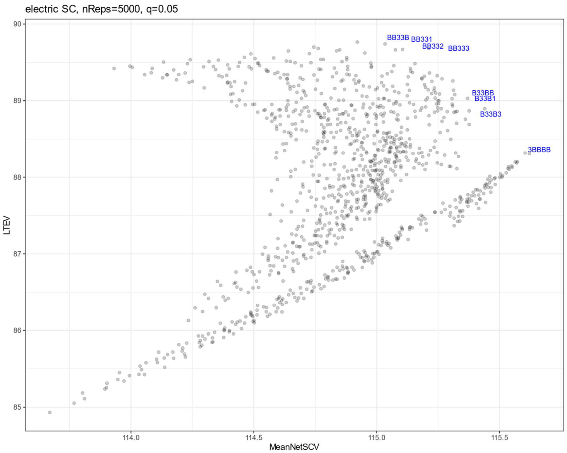
To better understand this multidimensional problem, consider Figure 2. Here, the x-axis represents NetSCV and the y-axis represents LTEV. The scatter plot shows the NetSCV and LTEV of every possible combination of the portfolios. Each point is labeled with the portfolio name, such as “B33BB”, where ‘B’ indicates no investment for a specific SCRM strategy, and the numeric value indicates the level of investment varying from 1 (lowest) to 3 (highest). This figure visualizes the trade-off between NetSCV and LTEV, allowing comparison of portfolios not just based on their expected value but also on their risk.
However, identifying the best portfolio is not simply a matter of applying multi-objective optimization methods. It requires careful interpretation of these quantitative measures in conjunction with the decision maker’s insights, business priorities, and an understanding of non-quantifiable factors that may affect the supply chain. These might include elements such as fluctuating market conditions, conflicting strategic business goals, or regulatory or internal constraints, among others.
For example, a portfolio that maximizes NetSCV might not necessarily be the best one if it also exposes the supply chain to higher risk, as indicated by a high VaR or CVaR. Likewise, a portfolio with the highest LTEV might not be optimal if it results in a negative PV. Hence, the decision maker must consider the trade-offs among these measures when choosing the best portfolio. In other words, VaR and CVaR are treated as loss-based downside-risk measures.
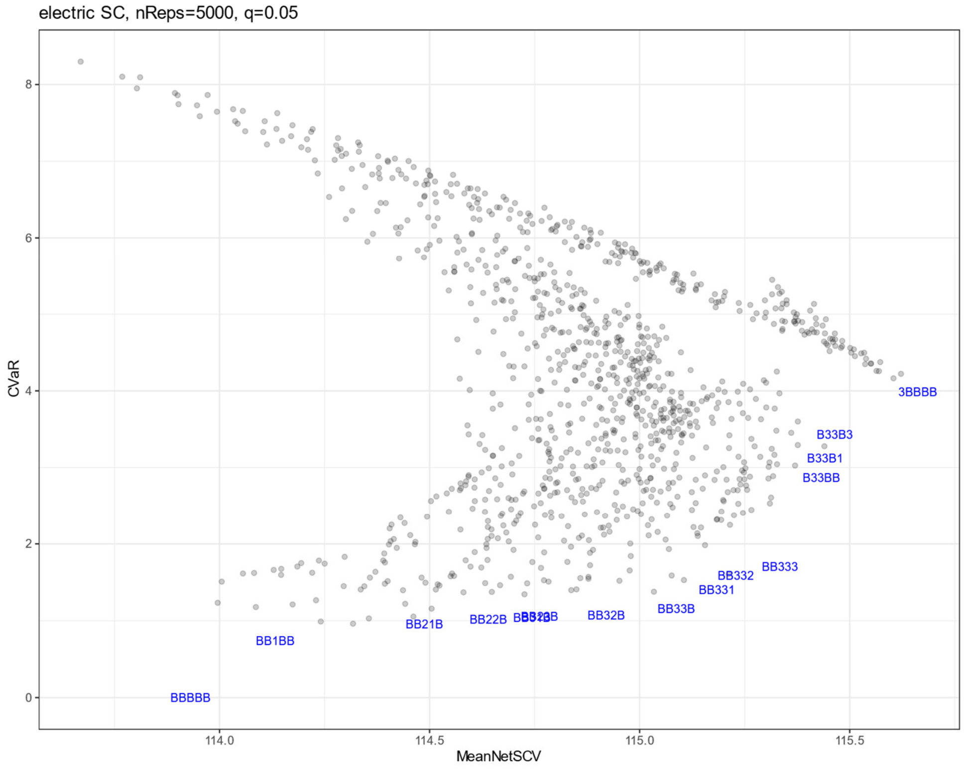
To better illustrate this, refer to Figure 3, which is similar to Figure 2, but here the y-axis represents CVaR. This figure allows us to see how each portfolio’s risk (CVaR) relates to its NetSCV, providing another important perspective when considering portfolio choice. Because lower VaR and CVaR values indicate lower exposure to severe disruption outcomes, the preferred direction is toward higher NetSCV and lower CVaR. The figure underscores that the decision maker must consider the trade-offs among these measures when choosing the best portfolio.
This process of determining the best-performing SCRM portfolio is essentially a multi-objective decision-making task that integrates quantitative performance measures with qualitative insights and judgment. It is crucial to recognize the importance of decision makers’ involvement and their ability to understand and interpret the results of the quantitative models in the context of their organization’s specific risk and business environment. It is this blend of quantitative analysis and qualitative judgement that ultimately leads to the selection of the best-performing SCRM portfolio.
The next section demonstrates the efficacy of genetic algorithms in SCRM portfolio selection, benchmarked against the Monte Carlo Search. The experiments demonstrate the capability of genetic algorithms that can provide diverse, near-optimal solutions to deal with the complex task of SCRM portfolio optimization. The subsequent details and insights gained from these experiments are intended to showcase the potential of genetic algorithms as a valuable tool for more informed and efficient decision-making in supply chain risk management.

4. Experiments

In order to test the effectiveness of using the genetic algorithm in the context of identifying the best-performing supply chain risk management (SCRM) portfolio for a given performance measure, two experiments are designed. The first aims to examine the comparative performance of the genetic algorithm (GA) and Monte Carlo Search (MCS) and shows the efficacy of GA in addressing the complex task of selecting an optimal SCRM portfolio that is tailored to specific risk and business environments. A second experiment is conducted to examine the diversity of near-optimal solutions generated by the GA and MCS. This aspect of the second experiment highlights the ability of the genetic algorithm to provide a range of diverse, high-performing SCRM portfolios that offer valuable decision support to managers.
The genetic algorithm (GA), inspired by the principles of natural selection and genetics, utilizes a population-based approach to search for near-optimal solutions in the complex solution space. On the other hand, Monte Carlo Search is a sampling-based optimization technique that leverages random sampling to explore the solution space and approximate optimal solutions. The GA is particularly effective in searching large, complex spaces where exact methods are computationally expensive. In this study, the GA is employed to identify high-performing SCRM portfolios in a more efficient manner compared to exhaustive and random search methods.
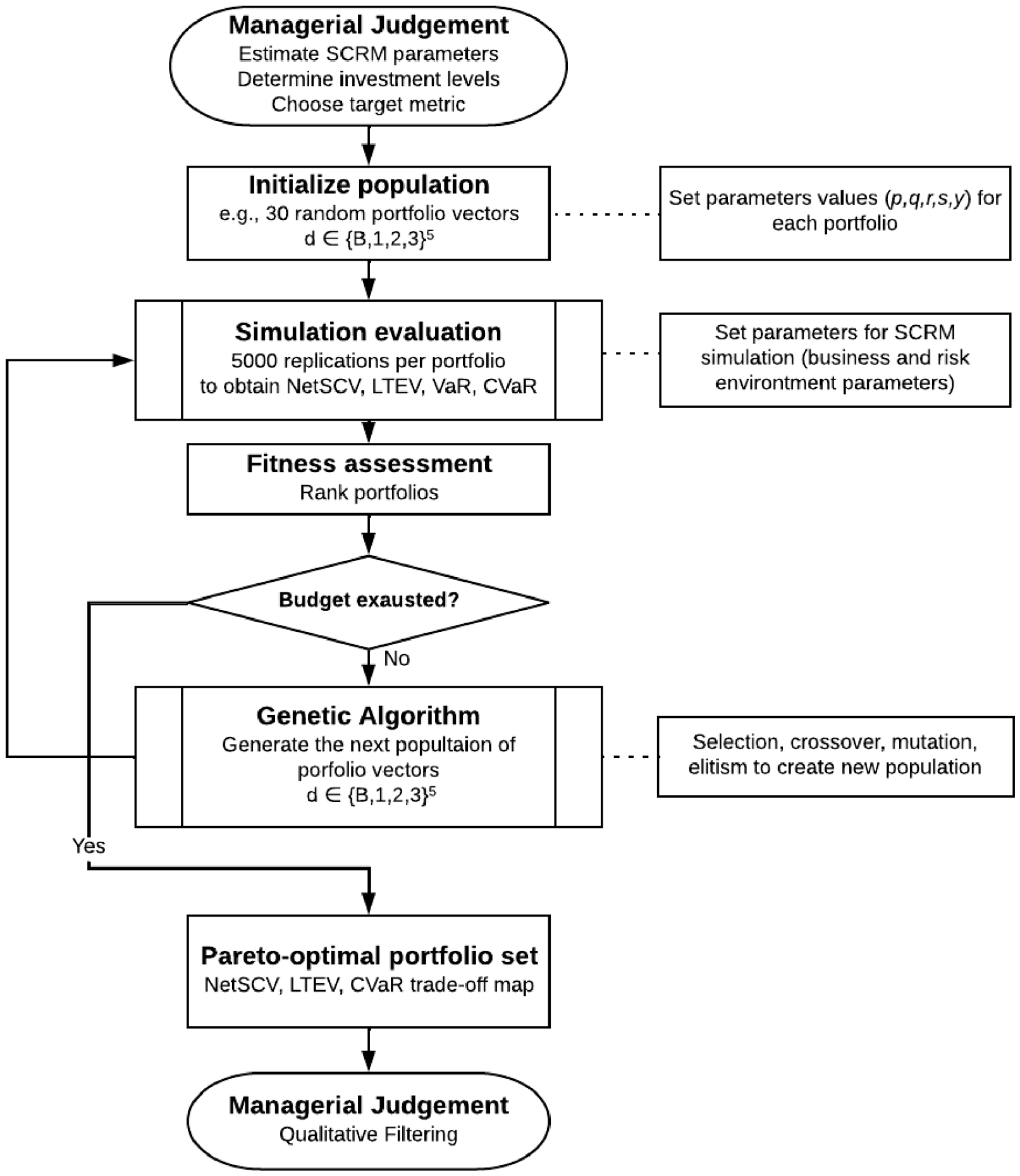
Figure 4 illustrates the iterative architecture of the GA-simulation optimization loop. Beginning with an initial population of 30 randomly generated portfolio vectors d   =   ( d p ,   d q ,   d r ,   d s ,   d y ) , each portfolio is evaluated by the stochastic simulation engine, which runs 5000 replications and returns the full multi-dimensional performance vector (NetSCV, PV, LTEV, VaR, CVaR). The role of the GA is to optimize on a single chosen performance metric, for example, NetSCV, using Gaussian rank selection, one-point crossover, and mutation, retaining the best portfolio via elitism. All evaluated portfolios and their full performance vectors are stored throughout the 256-evaluation budget. The near-Pareto trade-off map is not a direct output of the GA’s multi-objective search; rather, it emerges from the collection of diverse near-optimal solutions accumulated across evaluations. The solution diversity experiment in Section 4.3, in which mutation rates of 0.1, 0.35, and 0.6 are tested, controls the exploration-versus-exploitation balance and determines how structurally different the accumulated near-optimal portfolios are. Managerial judgment enters at two points: at initialization, in choosing the target performance metric and seeding the search, and at the final selection stage, where the near-Pareto portfolio menu is filtered using qualitative criteria.

4.1. Experimental Parameters for Genetic Algorithm

The GA operates on a population of potential solutions to the problem at hand—in this case, a population of potential SCRM portfolios. Each portfolio is represented as a string of parameters, akin to chromosomes in natural genetics, that signify the SCRM strategies used and their levels of implementation.
The GA begins with an initial population of 30 potential solutions, or portfolios, which are randomly generated. Each portfolio in the population is then evaluated based on the predefined performance measures, such as NetSCV, PV, LTEV, and CVaR. This evaluation represents the fitness of the portfolio in the context of the problem. The GA then uses these fitness values to guide the selection of portfolios for reproduction.
The algorithm prefers portfolios with higher fitness values but also allows for some randomness to maintain diversity. The selected portfolios are then recombined or crossed over to create offspring portfolios. This is followed by a mutation process, where certain elements of the offspring portfolios are randomly altered to introduce further diversity. The mutation rates tested are 0.1, 0.35, and 0.6. The offspring portfolios are then evaluated, and the process of selection, crossover, and mutation is repeated over multiple generations. In this study, the GA is run up to 256 evaluations. The GA also employs a mechanism known as elitism, where the best-performing portfolio from the current generation is guaranteed a place in the next generation. The elitism value is set to 1, ensuring that the best portfolio found thus far is always retained. The GA continues in this manner until a stopping criterion is met—either a maximum number of evaluations or a satisfactory performance level. The result is a set of high-performing, diverse SCRM portfolios that provide valuable decision support for supply chain managers. Finally, it should be noted that the GA requires a specified number of test replications per portfolio to ensure accurate performance assessment. The test replication value is set to 100. Detailed experimental settings are provided in Table 4.
After establishing the GA parameters, the first experiment evaluates the GA’s effectiveness in finding near-optimal solutions.

4.2. Assessing Portfolio Robustness Across Diverse Risk Metrics

To evaluate SCRM portfolios, simulation data are generated using the same simulation framework as detailed in [3]. The business environment parameters, risk environment parameters, and SCRM effectiveness parameters for the baseline SCRM are provided in Table A1 of Appendix A.
The five parameters (p, q, r, s, y) take discrete values between 0 and 1, representing increasing levels of investment effectiveness. The baseline (1.0) corresponds to no new investment, while progressively lower values correspond to greater effectiveness. For investment level l v { 1,2 , 3 } , parameter values are set as:
p a r a m e t e r   v a l u e   ( l v )   =   b a s e V a l u e   +   ( a d v V a l u e     b a s e V a l u e )   ×   l v   / ( l v +   1 )
where baseValue = 1.0 and advValue is the maximum effectiveness for that parameter. The resulting values are shown in Table A2.
Because of the stochastic nature of risk events and its impact on the supply chain, a large number of SCRM simulation replications is used to determine overall SCRM performance. Instead of examining mean-based performance, such as expected net SCV, tail-probability-based performance, such as CVaR, is also used. The large number of replications can provide reliable probability distributions of an SCRM outcome, which allow accurate calculation of tail-probability-based measures.
For the illustrative five-dimensional problem space with four investment levels per parameter, the total number of combinations equals 4 5 = 1024 candidate portfolios. A full enumeration using a workstation with a 48-core CPU (Dual 24-Core Intel Xeon Gold 6248R CPU @3.00 GHz) requires approximately 0.5 h of continuous execution because each portfolio must undergo 5000 stochastic simulation replications to stabilize the tail-risk distributions. While full enumeration is mathematically feasible at this specific scale, it becomes computationally intractable as the model scales. Adding just three additional strategic choices and increasing parameter granularity to 8 levels expands the search space exponentially to 8 8 = 16,777,216 combinations, which would require over 341 days of computing time. This highlights the practical necessity of utilizing heuristic search methods like the GA for larger real-world problems. Empirically validating the GA’s performance at these larger scales, for example, with 10,000 or 100,000 candidate portfolios, is identified as an important direction for future research.
This experiment compares the performance of the Full Search (FS), Genetic Algorithm (GA), and Monte Carlo Search (MCS) methods in identifying the best-performing SCRM portfolios. The FS method evaluates all 1024 possible portfolios to find the true optimum, serving as a benchmark. To test efficiency, both the GA and MCS were given a limited budget of 256 evaluations (25% of the total search space).
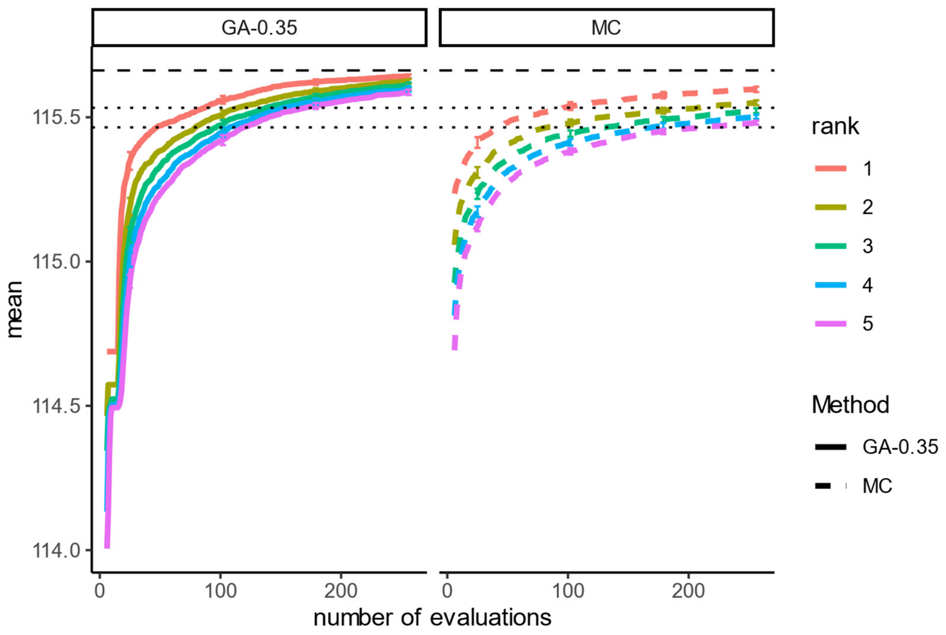
The results, summarized in Table 5, confirm that the GA consistently identifies high-performing portfolios, achieving at least 99.55% of the FS optimum, evidence that the GA consistently delivers “satisficing” solutions that a manager can act on with confidence, without requiring exhaustive enumeration. Importantly, the GA’s advantage is most pronounced for the tail-risk measures most consequential to risk-averse managers. For CVaR, the GA reaches 100% of optimal versus 76.23% for MCS, a significant gap that could represent a material difference in downside exposure under a severe disruption scenario.
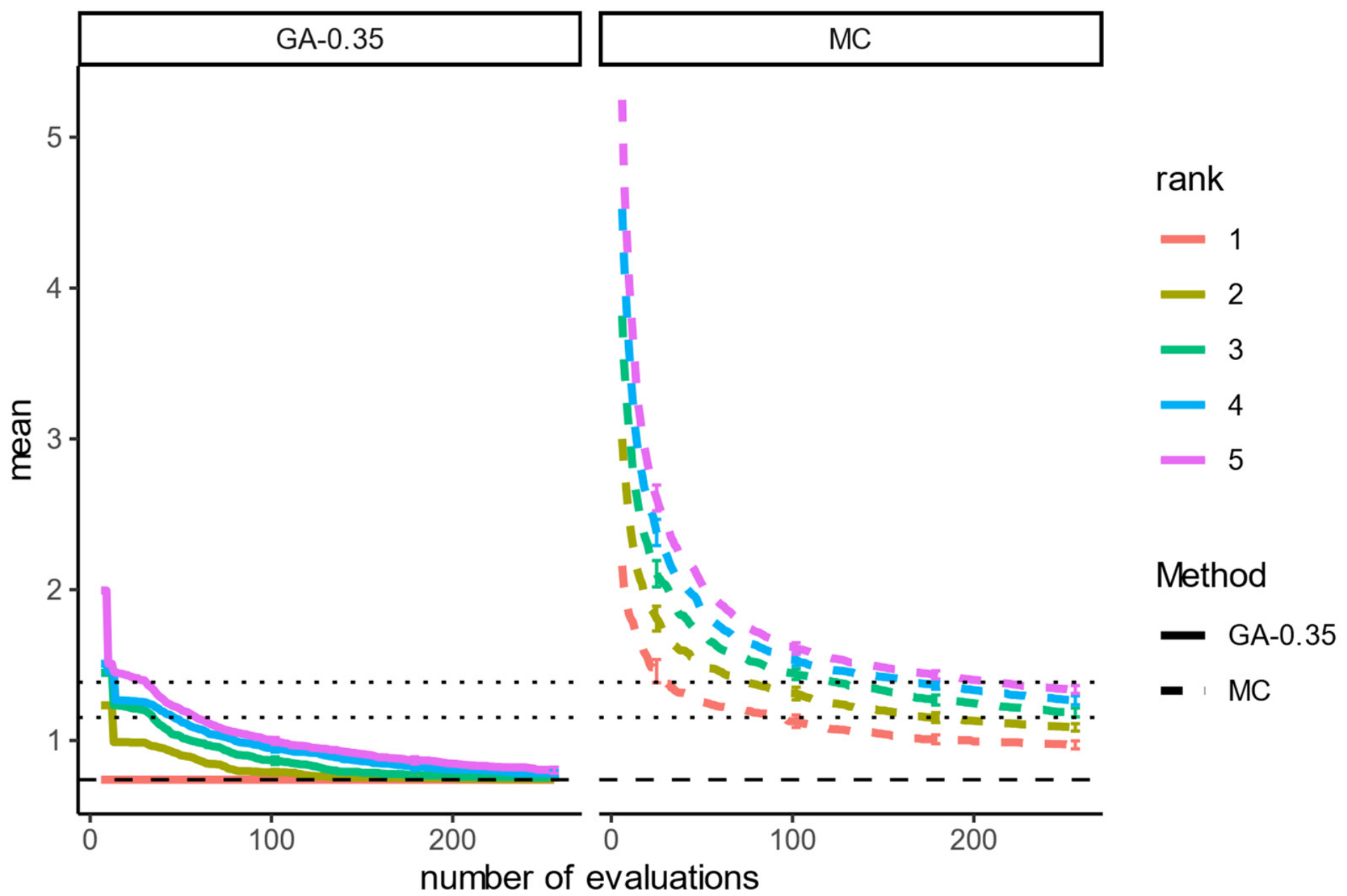
Furthermore, the convergence plots in Figure 5 and Figure 6 illustrate the speed with which the GA delivers actionable insight. In a strategic planning context, where managers may need to evaluate portfolio options within the span of a single meeting or planning session, the GA’s ability to identify a high-quality portfolio menu within the first 50–100 evaluations is practically significant. Rather than waiting for exhaustive search to complete, decision-makers receive rapid feedback on the structure of the solution space, enabling timely and informed discussion.
Building on the finding that the GA can efficiently identify optimal portfolios, the second experiment investigates another key capability: its ability to generate a diverse set of high-performing solutions for strategic consideration.

4.3. Generating Strategic Options for Adaptive Risk Management

In addition to finding a single best solution, it is often more valuable for managers to have a set of diverse, high-performing portfolios to choose from. This experiment assesses the ability of the GA and MCS to generate such a pool of solutions. The top 5 solutions found by each method in each of the 100 runs are analyzed by measuring both the number of “near-optimal” solutions (defined as portfolios performing within 5% of the true optimum) and their structural diversity (average pairwise Euclidean distance). For CVaR, near-optimal solutions were identified using an empirical distribution-based threshold rather than a ratio to the true optimum. Because a low CVaR is preferred, solutions falling within the lowest 1% of the portfolio CVaR distribution were classified as near-optimal. Table 6 shows that the GA with the mutation rates of 0.1 and 0.35 consistently identifies all five near-optimal solutions across runs. Even at the highest mutation rate of 0.6, the GA identifies an average of at least 4.32 near-optimal solutions while maintaining structural diversity comparable to that of MCS.
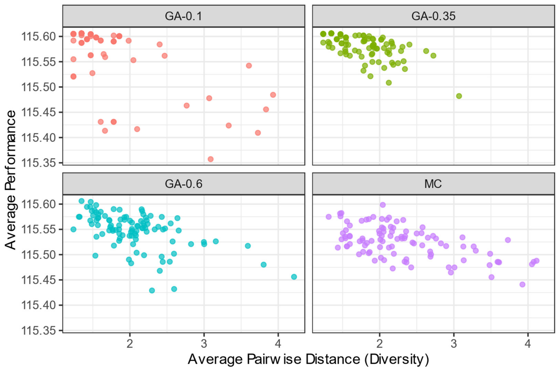
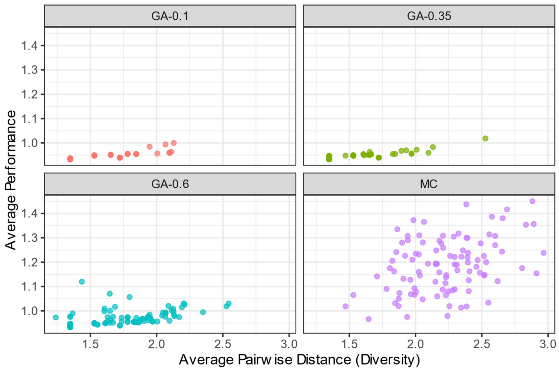
The results reveal that the mutation rate gives managers direct control over the breadth of the portfolio menu they receive. A low mutation rate (GA-0.1) produces a focused set of high-performing, structurally similar alternatives, which is well suited when a manager has high confidence in the risk environment and seeks to refine among closely related strategies. A higher mutation rate (GA-0.6) provides a broader menu of structurally different strategies, surfacing alternatives that may differ substantially in which levers they engage. For example, one portfolio may concentrate investment in prevention (p) and detection (y), while another prioritizes resilience (r) and recovery rate (s). This wider menu is particularly valuable when the risk environment itself is uncertain; for example, when managers are unsure whether a disruption will be short and sharp (favoring fast recovery) or prolonged and structural (favoring resilience and supplier diversification). In such cases, having a set of structurally diverse portfolios on hand allows managers to deliberate across genuinely different strategic options rather than choosing among minor variations in the same approach.
The optimality vs. diversity plots in Figure 7 and Figure 8 show that lower mutation rates (e.g., GA-0.1) tend to produce a tight cluster of high-performing but less diverse solutions (a strategy of exploitation). As the mutation rate increases, the diversity of the solutions also increases, but often at the cost of a slight decrease in average performance (a strategy of exploration). MCS, being a random search, naturally produces the most diverse solutions but at a significant cost to performance, finding far fewer near-optimal portfolios for risk-based metrics like VaR and CVaR. This demonstrates the GA’s key advantage: it can be tuned to provide managers with a set of high-quality solutions that balance optimality and diversity according to their strategic needs.
The practical implications of these experimental results are discussed in the following section.

5. From Optimization to Strategic Exploration

The experimental results reframe what SCRM optimization means in practice. Rather than converging on a single algorithmic solution, the framework transforms SCRM from a search for a single answer into a strategic exercise in informed decision-making, one in which the manager, not the algorithm, makes the final call. This section interprets the findings through a managerial lens, focusing on what the results reveal about how ESG-aware, risk-averse decision-makers can select and adapt SCRM portfolios under conditions of deep uncertainty—conditions exemplified by scenarios such as geopolitical disruptions to the Strait of Hormuz, where the risk event is known, the timing is not, and the magnitude is deeply uncertain.

5.1. Keeping the Manager in the Loop

The primary managerial value of the framework is not computational efficiency but the quality of the decision space it reveals. In traditional optimization, a single recommended solution is presented to the manager, who must accept it or seek alternatives from scratch. Under conditions of deep uncertainty, this is not appropriate because if the model’s assumptions change, as they inevitably do when ESG risks materialize, a single-point solution offers no fallback. The present framework deliberately generates a structured ensemble of diverse, high-performing alternatives, so that managers already hold a portfolio of contingency strategies when conditions shift. Critically, this design keeps the manager in the loop. Rather than replacing managerial judgment with an automated recommendation, the framework empowers decision-makers to apply their own risk attitudes and qualitative knowledge to a curated set of viable options.
By adjusting the mutation rate, decision-makers can readily switch from “exploitation,” i.e., refining a known strategy to obtain the optimal outcome, to “exploration,” which uncovers structurally different portfolios that might be more resilient to unforeseen institutional or environmental regulations, or internal organizational constraints that are difficult to parameterize in a simulation.
As shown in the optimality vs. diversity plots (Figure 7 and Figure 8), a lower mutation rate (e.g., 0.1) prompts the GA to focus on exploitation, yielding a tight cluster of high-performing but structurally similar portfolios. Conversely, a higher mutation rate (e.g., 0.6) encourages exploration, generating a more diverse set of solutions that may have a slightly wider performance distribution. Managers can select a higher-performing, focused portfolio if they have high confidence in their model parameters, or they can opt for a more diverse set of solutions to facilitate strategic discussions and qualitative assessments, especially when non-quantifiable factors are at play. In either case, the choice of mutation rate is itself a managerial decision—a reflection of how much confidence the manager has in the model assumptions and how much strategic flexibility they wish to preserve.

5.2. Navigating Multi-Dimensional Trade-Offs

A central challenge for ESG-aware supply chain risk managers is that different stakeholders (e.g., shareholders, regulators, ESG rating agencies, and operational teams) often prioritize different risk dimensions. Shareholders may focus on expected return (NetSCV), while regulators and ESG auditors may be more concerned with worst-case outcomes (CVaR). Rather than resolving this tension algorithmically, the framework surfaces it explicitly, allowing each stakeholder group to identify the portfolios most aligned with their priorities. The ability to identify near-optimal solutions across all these metrics simultaneously allows for the construction of a Pareto frontier. Figure 2 and Figure 3 serve as strategic dashboards where decision-makers can visualize the cost of resilience, for instance, exactly how much expected value (NetSCV) must be sacrificed to achieve a safer level of downside risk (LTEV). A dashboard with a limited number of superior solutions enables decision-makers to consider that trade-off consciously rather than having it resolved by default within a single-objective model.
Because the GA identifies a set of robust alternatives rather than one “best” answer, the framework supports adaptive decision-making. If new information emerges or supply chain conditions shift, managers already have an ensemble of high-performing strategies to pivot toward, rather than starting the optimization process from scratch. This is especially valuable for ESG risk governance, where the triggering event, such as a Strait of Hormuz disruption, a climate-driven port closure, or a supplier human rights violation, is often anticipated in general terms but uncertain in timing and magnitude. A manager who has already explored the Pareto frontier can quickly identify which portfolio in their menu best matches the materialized risk profile, rather than launching a new optimization under crisis conditions. In this way, the framework functions less as a decision-maker and more as a strategic advisor that organizes and presents the landscape of options, while leaving the final judgment to the manager who understands the full organizational context.

6. Conclusions, Limitations, and Future Research

This study presents a decision-centric framework for sustainable SCRM portfolio selection, designed to support supply chain risk managers navigating the deep uncertainties of the modern ESG risk environment. By parameterizing risk management strategies across five time-dependent dimensions, prevention, vulnerability, resilience, recovery rate, and detection delay, and evaluating candidate portfolios through multiple performance measures, including both mean-based metrics and tail-risk measures such as LTEV and CVaR, the framework produces a rich Pareto frontier of alternatives that managers can interpret, compare, and filter through qualitative ESG and institutional judgment. The genetic algorithm serves as the framework’s efficient search engine, enabling this decision landscape to be generated without exhaustive enumeration. Rather than seeking an optimal solution, the framework embraces a satisficing logic, generating a set of high-quality alternatives that are good enough to act on and diverse enough to accommodate the heterogeneous risk attitudes and qualitative constraints that real managers bring to the decision. The core finding is not that one algorithm outperforms another, but that robust SCRM governance requires presenting managers with a structured set of diverse, high-quality alternatives, and that the exploration-exploitation dial embedded in the framework gives managers active control over the breadth of that portfolio menu, reflecting their own level of confidence in the model assumptions and the degree of strategic flexibility they wish to preserve.
Despite the promising results, this study has several limitations. First, the model relies on the ability to estimate a number of parameters to characterize the risk environment and strategy effectiveness. While this can be achieved through a combination of historical data and expert opinion, this process can be challenging and subject to biases. Second, the simulation models a generalized supply chain; the specific portfolio effects and optimal strategies would undoubtedly vary for different industries, supply chain structures, and risk profiles. The interactions between strategies were also modeled as multiplicative, while real-world synergies could be more complex. Finally, while the simulation framework includes a linear cost function scaled to each strategy’s simulated value contribution, the present experiments did not activate it because per-strategy cost proportions were not available for the generalized supply chain setting. A practitioner with access to these estimates can immediately incorporate cost into all performance measures without structural changes to the framework.
The limitations of this study open several avenues for future research. An immediate next step would be to incorporate the costs associated with implementing and executing SCRM strategies into the optimization framework, allowing for an analysis based on return on investment (e.g., ROPI). Another valuable extension would be to apply this methodology to a specific real-world case study, using company data to validate the model and generate actionable insights. Scaling the experimental design to larger portfolio spaces, for example, by increasing the number of risk management strategies or the granularity of investment levels, would also allow assessment of how GA performance changes with problem size and provide stronger evidence of the framework’s practical reach. The framework is designed to accommodate this directly: the simulation engine, GA search, and performance dashboard are modular components that accept industry-calibrated parameter inputs without structural modification, making application to a specific supply chain context a natural next step. Further research could also explore more complex, non-linear interactions between risk management strategies and investigate the use of other metaheuristic algorithms. Finally, integrating this quantitative approach with qualitative frameworks like the Analytical Hierarchy Process (AHP) could lead to a more holistic decision support system that formally incorporates managerial judgment alongside simulation results.

Author Contributions

Conceptualization, K.K., S.P. and R.L.K.; Methodology, K.K., S.P. and R.L.K.; Software, K.K. and S.P.; Validation, K.K., S.P. and R.L.K.; Formal analysis, K.K., S.P. and R.L.K.; Investigation, K.K., S.P. and R.L.K.; Writing—original draft, K.K., S.P. and R.L.K.; Writing—review and editing, K.K., S.P. and R.L.K.; Funding acquisition, S.P. All authors have read and agreed to the published version of the manuscript.

Funding

This research was funded in part by the Belk College of Business at the University of North Carolina at Charlotte through the 2019 Belk College Summer Research Grant Program.

Institutional Review Board Statement

Not applicable.

Informed Consent Statement

Not applicable.

Data Availability Statement

The raw data supporting the conclusions of this article will be made available by the authors on request.

Acknowledgments

The first author would like to express sincere gratitude to the Department of Business Information Systems and Operations Management at the University of North Carolina at Charlotte for the support during their time as a visiting researcher from August 2018 to July 2019, during which most of this work was conducted.

Conflicts of Interest

The authors declare no conflicts of interest.

Appendix A. SCRM Simulation Model and Parameters

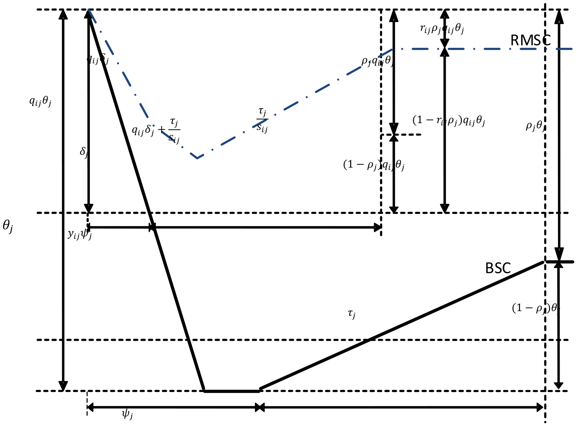
This appendix provides a formal description of the stochastic simulation model underlying the present framework, following Kumar and Park [3]. Supply chain value (SCV) is modeled as a jump-diffusion process combining three components: a continuous drift term ( α ) representing the long-term trend in supply chain performance, a Wiener noise term ( σ z ) capturing short-term perturbations, and discrete jump events representing sudden changes in value. Positive jumps, such as demand surges, arrive at rate λ k and increase SCV proportionally; negative jumps—risk materializations of type j—arrive at rate λ j and reduce SCV by a damage proportion θ j drawn from a lognormal distribution. Following a risk event, SCV recovers after a detection delay ψ j and increases the recovery rate τ j until reaching a residual retained-damage level ρ j θ j , which may reflect permanent or long-term value loss. Figure A1 illustrates this disruption-recovery trajectory and shows how the five effectiveness parameters, p, q, r, s, and y, shape each phase of the cycle: p scales the arrival rate λ j , reducing how frequently risk events materialize; q scales the initial damage θ j , limiting the severity of impact; y scales the detection delay ψ j , accelerating the onset of recovery; s scales the recovery rate τ j , determining how quickly SCV rebounds; and r scales the retained damage ρ j θ j , governing the completeness of recovery. All effectiveness parameters are modeled as beta-distributed random variables estimated from three-point managerial inputs—optimistic, most-likely, and pessimistic—except for p, which is a single Bernoulli scalar representing the probability that a prevention strategy fails to stop a risk event. Table A1 summarizes all model parameters, their underlying stochastic processes, and the distributions used in the simulation. Table A2 reports the specific parameter values used in the experiments of the present study. Table A3 maps the discrete investment levels (B,1,2,3) to the corresponding effectiveness parameter values for each of the five dimensions.
Figure A1. The effect of SCRM parameters on SCV (adapted from [3]).
Sustainability 18 06863 g0a1
Table A1. SCRM Model parameters (adapted from [3]).
TypeParameterRandom Variable and/or Underlying Stochastic ProcessDistribution Used in Simulation Model
Business Environment T : planning horizon; simulation period.Constant
α : drift rateConstant
σ z : instantaneous variance d z t , Wiener Normal
λ k : arrival rate of positive jump type k A k ( t ) : PoissonExponential for interarrival time
μ k , σ k : scale and shape parameters of positive jump size x k , ln x k ~   N ( μ k ,   σ k 2 ) θ k ( t ) = x k S C V ( t ) Lognormal for x k
Risk Environment λ j : arrival rate of risk type j A j ( t ) : PoissonExponential
μ j ,   σ j : scale and shape parameters of negative jump proportion x j , ln x j ~   N ( μ j ,   σ j 2 ) θ j ( t ) = ( 1 x j ) S C V ( t ) Lognormal for x j
ρ j m , ρ j a , ρ j b : most likely, optimistic, and pessimistic estimates of retained damage ρ j Beta
τ j m ,   τ j a ,   τ j b : most likely, optimistic, and pessimistic estimates of recovery rate τ j Beta
ψ j m ,   ψ j a ,   ψ j b : most likely, optimistic, and pessimistic estimates of recovery delay ψ j Beta
SCRM Action Effectiveness p i j : probability of not preventing a damage j with RM strategy i (i.e., ineffectiveness of RM strategy i on risk j ) X (1 or 0)Bernoulli
q i j m , q i j a , q i j b : most likely, optimistic, and pessimistic estimates of effect of RM strategy i on θ j q i j Beta
r i j m , r i j a , r i j b : most likely, optimistic, and pessimistic estimates of effect of RM strategy i on ρ j r i j Beta
s i j m , s i j a , s i j b : most likely, optimistic, and pessimistic estimates of effect of RM strategy i on τ j s i j Beta
y i j m ,   y i j a ,   y i j b : most likely, optimistic, and pessimistic estimates of effect of RM strategy i   on ψ j y i j Beta
Table A2. Parameter values used for the SCRM simulation.
TypeParameterValue
Business EnvironmentT: planning horizon2 years
α : drift rate−10% per year
σ z : instantaneous variance5% per year
SCV(0): initial SC value$100 (million)
k: type of positive event1, 2
{ λ k } : arrival rate of positive event k{2, 10}
{ μ k } : average jump size for event k{ln(1.10), ln(1.02)}
{ σ k } : variance of jump size for event k{0.01, 0.005}
Risk Environmentj: risk type1, 2, 3, 4, 5
{ λ j } : arrival rate of risk event j{2, 10, 0.5, 0.2, 12}
{ μ j } : average damage ( θ j ) for event j{ln(0.90), ln(0.99), ln(0.90), ln(0.90), ln(0.95)}
{ σ j } : variance of θ j for event j{0.03, 0.002, 0.01, 0.01, 0.005}
{ t δ j m } , { t δ j a } , { t δ j b } : damage period estimates for event j (used to derive most likely, optimistic, pessimistic estimates of δ j ){1, 1, 10, 50, 10},
{0.5, 0.5, 5, 20, 5},
{3, 5, 20, 100, 30}
{ t τ j m } , { t τ j a } , { t τ j b } : recovery time estimates for event j (used to derive most likely, optimistic, pessimistic estimates of τ j ){60, 0.5, 50, 100, 20},
{10, 0, 10, 20, 5},
{100, 10, 100, 200, 60}
{ ρ j m },{ ρ j a },{ ρ j b }: most likely, optimistic, pessimistic values of post recovery damage{0.1, 0.05, 0.5, 0.2, 0.2},
{0.01, 0.01, 0.01, 0.01, 0.01},
{0.5, 0.5, 0.8, 0.5, 0.5}
{ ψ j m },{ ψ j a },{ ψ j b }: most likely, optimistic, pessimistic value of recovery delay{30, 0.5, 20, 30, 5},
{0, 0, 0, 0, 0},
{180, 2, 140, 160, 50}
SCRM Action
Effectiveness
i: risk management action (basic)1, 2, 3, 4, 5
p i j : effectiveness on λ j 0.5 for i = 1, and 1.0 otherwise.
q i j m , q i j a , q i j b : effectiveness on θ j 0.9, 0.5, 1.0 for i = 2, and 1, 1, 1 otherwise
r i j m , r i j a , r i j b : effectiveness on ρ j 0.9, 0.5, 1.0 for i = 3, and 1, 1, 1 otherwise
s i j m , s i j a , s i j b : effectiveness on τ j 0.9, 0.5, 1.0 for i = 4, and 1, 1, 1 otherwise
y i j m , y i j a , y i j b : effectiveness on ψ j 0.9, 0.5, 1.0 for i = 5, and 1, 1, 1 otherwise
Table A3. Parameter values used for investment level.
Investment Level pqrsy
B (baseline)1.0001.0001.0001.0001.000
10.7500.9500.9500.9500.950
20.6670.9330.9330.9330.933
30.6250.9250.9250.9250.925
Note: Values derived using the formula in Section 4.2; advValue = 0.5 for p (single scalar); advValue = 0.9 (most likely estimate) for q, r, s, y.

References

  1. Heckmann, I.; Comes, T.; Nickel, S. A critical review on supply chain risk–Definition, measure and modeling. Omega 2015, 52, 119–132. [Google Scholar]
  2. Dunke, F.; Heckmann, I.; Nickel, S.; Saldanha-da-Gama, F. Time traps in supply chains: Is optimal still good enough? Eur. J. Oper. Res. 2018, 264, 813–829. [Google Scholar] [CrossRef]
  3. Kumar, R.L.; Park, S. A portfolio approach to supply chain risk management. Decis. Sci. 2019, 50, 210–244. [Google Scholar]
  4. Macdonald, J.R.; Zobel, C.W.; Melnyk, S.A.; Griffis, S.E. Supply chain risk and resilience: Theory building through structured experiments and simulation. Int. J. Prod. Res. 2018, 56, 4337–4355. [Google Scholar] [CrossRef]
  5. Cox, L.A., Jr. Confronting deep uncertainties in risk analysis. Risk Anal. Int. J. 2012, 32, 1607–1629. [Google Scholar] [CrossRef]
  6. Tang, C.S. Perspectives in supply chain risk management. Int. J. Prod. Econ. 2006, 103, 451–488. [Google Scholar] [CrossRef]
  7. Ho, W.; Zheng, T.; Yildiz, H.; Talluri, S. Supply chain risk management: A literature review. Int. J. Prod. Res. 2015, 53, 5031–5069. [Google Scholar] [CrossRef]
  8. Emrouznejad, A.; Abbasi, S.; Sıcakyüz, Ç. Supply chain risk management: A content analysis-based review of existing and emerging topics. Supply Chain Anal. 2023, 3, 100031. [Google Scholar] [CrossRef]
  9. Pournader, M.; Kach, A.; Talluri, S. A review of the existing and emerging topics in the supply chain risk management literature. Decis. Sci. 2020, 51, 867–919. [Google Scholar] [CrossRef] [PubMed]
  10. Hendricks, K.B.; Singhal, V.R. Association between supply chain glitches and operating performance. Manag. Sci. 2005, 51, 695–711. [Google Scholar] [CrossRef]
  11. Hendricks, K.B.; Singhal, V.R. An empirical analysis of the effect of supply chain disruptions on long-run stock price performance and equity risk of the firm. Prod. Oper. Manag. 2005, 14, 35–52. [Google Scholar] [CrossRef]
  12. March, J.G.; Shapira, Z. Managerial perspectives on risk and risk taking. Manag. Sci. 1987, 33, 1404–1418. [Google Scholar] [CrossRef]
  13. Peck, H. Reconciling supply chain vulnerability, risk and supply chain management. Int. J. Logist. Res. Appl. 2006, 9, 127–142. [Google Scholar] [CrossRef]
  14. Wakolbinger, T.; Cruz, J.M. Supply chain disruption risk management through strategic information acquisition and sharing and risk-sharing contracts. Int. J. Prod. Res. 2011, 49, 4063–4084. [Google Scholar] [CrossRef]
  15. Uryasev, S.; Sarykalin, S.; Serraino, G.; Kalinchenko, K. VaR vs CVaR in risk management and optimization. In Proceedings of the CARISMA Conference, La Grande Motte, France, 19–22 September 2010; Available online: https://www.researchgate.net/publication/200798611_Value-_at-Risk_vs_Conditional_Value-at-Risk_in_Risk_Management_and_Optimization (accessed on 30 June 2026).
  16. Acerbi, C.; Tasche, D. On the coherence of expected shortfall. J. Bank. Financ. 2002, 26, 1487–1503. [Google Scholar] [CrossRef]
  17. Hult, G.T.M.; Craighead, C.W.; Ketchen, J.; David, J. Risk uncertainty and supply chain decisions: A real options perspective. Decis. Sci. 2010, 41, 435–458. [Google Scholar] [CrossRef]
  18. Aven, T. On how to deal with deep uncertainties in a risk assessment and management context. Risk Anal. 2013, 33, 2082–2091. [Google Scholar] [CrossRef] [PubMed]
  19. Simon, H.A. A behavioral model of rational choice. Q. J. Econ. 1955, 69, 99–118. [Google Scholar] [CrossRef]
  20. Aguilar-Rivera, R.; Valenzuela-Rendón, M.; Rodríguez-Ortiz, J. Genetic algorithms and Darwinian approaches in financial applications: A survey. Expert Syst. Appl. 2015, 42, 7684–7697. [Google Scholar] [CrossRef]
  21. Meena, P.L.; Sarmah, S.P. Multiple sourcing under supplier failure risk and quantity discount: A genetic algorithm approach. Transp. Res. Part E Logist. Transp. Rev. 2013, 50, 84–97. [Google Scholar] [CrossRef]
  22. Altiparmak, F.; Gen, M.; Lin, L.; Paksoy, T. A genetic algorithm approach for multi-objective optimization of supply chain networks. Comput. Ind. Eng. 2006, 51, 196–215. [Google Scholar] [CrossRef]
  23. Nooraie, V.; Fathi, M.; Narenji, M.; Parast, M.M.; Pardalos, P.M.; Stanfield, P. A multi-objective model for risk mitigating in supply chain design. Int. J. Prod. Res. 2020, 58, 1338–1361. [Google Scholar]
  24. Sawik, T. Selection of optimal countermeasure portfolio in IT security planning. Decis. Support Syst. 2013, 55, 156–164. [Google Scholar] [CrossRef]
  25. Malcolm, D.G.; Roseboom, J.H.; Clark, C.E.; Fazar, W. Application of a technique for research and development program evaluation. Oper. Res. 1959, 7, 646–669. [Google Scholar] [CrossRef]
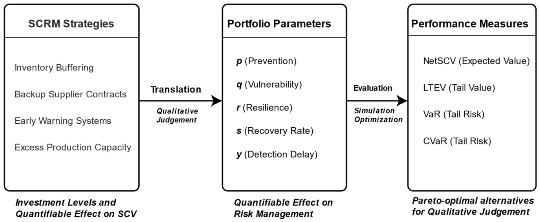
Figure 1. Conceptual framework of the decision-support approach for SCRM portfolio selection.
Sustainability 18 06863 g001
Figure 2. Trade-off between NetSCV and LTEV in SCRM portfolios.
Sustainability 18 06863 g002
Figure 3. Trade-off between NetSCV and CVaR in SCRM portfolios.
Sustainability 18 06863 g003
Figure 4. Iterative architecture of the GA-simulation optimization loop.
Sustainability 18 06863 g004
Figure 5. Optimality of Top 5 Solutions for NetSCV.
Sustainability 18 06863 g005
Figure 6. Optimality of Top 5 Solutions for CVaR.
Sustainability 18 06863 g006
Figure 7. Optimality vs. Diversity of Top 5 Solutions (NetSCV).
Sustainability 18 06863 g007
Figure 8. Optimality vs. Diversity of Top 5 Solutions (CVaR).
Sustainability 18 06863 g008
Table 1. Quantifying Risk and Risk Management Effectiveness (Adapted from [3]).
Risk CharacteristicQuantifiable Effect on SCVQuantifiable Effect of Risk Management
Detection of triggering eventElapsed time between detection of triggering event (e.g., supplier problem) and start of recovery (recovery delay)Reduced recovery delay (due to early warning/detection)
Occurrence of risk eventsArrival rate of risk materializationReduced arrival rate
VulnerabilityReduction in supply chain value (damage) due to risk materialization as proportion of original valueReduced damage
Recovery timeRecovery time (from start of recovery to completion)Reduced recovery time or increased recovery rate
ResilienceLevel of retained damage after recovery is complete (level of recovery) as a proportion of the original value before risk materialization.Reduced retained damage
Table 2. Examples of SCRM Portfolio Parametrization.
PortfolioConstituent StrategiesDerivation of ParametersParametric Vector
(p, q, r, s, y)
BasicNo new
investment
Represents the baseline where all parameters have a value of 1.00, indicating no additional RM effectiveness.(1, 1, 1, 1, 1)
Portfolio 1Finished Goods Inventory (FGI) + Early Warning SystemFGI reduces damage by 40% (q = 0.6). Early Warning reduces event likelihood by 20% (p = 0.8) and delay by 30% (y = 0.7).(0.8, 0.6, 1, 1, 0.7)
Portfolio 2Excess Capacity +
Backup Supplier Contract
Excess Capacity improves the recovery rate by 50% (s = 0.50). Backup Supplier reduces retained damage by 40% (r = 0.60). The strategies have a multiplicative synergy on recovery rate, so s becomes 0.5 times (1 − 0.20) = 0.4.(1, 1, 0.6, 0.4, 1)
Table 3. Mathematical formulation of the SCRM optimization problem.
Formulation ElementsDescriptionNotation
Decision variables Investment levels for each SCRM effectiveness parameter l p , l q ,   l r ,   l s ,   l y   { B ,   1 ,   2 ,   3 }  
SCRM effectiveness parameters Each effectiveness parameter is determined by the corresponding investment level. (see Section 4.2) p = f p ( l p   )
q = f q ( l q   )
r = f r (   l r   )
s = f s (   l s   )
y = f y (   l y   )
Competing objectivesCompeting objectives, such as NetSCV and CVaR, are stochastically evaluated through the simulation-optimization engine based on the decision variables, providing a Pareto-optimal menu for further qualitative managerial evaluation. max l p , l q ,   l r ,   l s ,   l y N e t S C V ( p ,   q ,   r , s , y )
max l p , l q ,   l r ,   l s ,   l y L T E V ( p ,   q ,   r , s , y )
mi n l p , l q ,   l r ,   l s ,   l y V a R ( p ,   q ,   r , s , y )
mi n l p , l q ,   l r ,   l s ,   l y C V a R ( p ,   q ,   r , s , y )
Table 4. Implementation details of the GA and the MCS.
CategoryConfigurationValue
Genetic AlgorithmPopulation size30
RepresentationBinary
Chromosome length10
SelectionGaussian rank selection
CrossoverOne-point crossover
Mutation rate0.1/0.35/0.6
Elitism1
Number of evaluations256
Monte Carlo SearchNumber of evaluations256
Table 5. Optimality comparisons for four SCRM performance metrics.
NetSCVPVLTEVCVaR
MethodBest% OptimalBest% OptimalBest% OptimalBest% Optimal
Full Search115.66100%15.25100%89.82100%0.74100%
Genetic Algorithm115.6499.98%15.1899.55%89.8199.98%0.74100%
Monte Carlo Search115.6099.94%14.9497.96%89.7499.91%0.9776.23%
Table 6. Solution Quality and Solution Diversity.
NetSCVPVLTEVCVaR
MethodCountDiversityCountDiversityCountDiversityCountDiversity
GA-0.15.01.634.991.565.01.584.971.50
GA-0.355.01.734.911.725.01.674.991.48
GA-0.65.02.054.322.005.01.904.651.73
MC5.02.322.612.185.02.182.282.23
Note: Count refers to the average number of near-optimal solutions; Diversity refers to the average pairwise Euclidean distance; Averages are calculated from 100 test runs.
Disclaimer/Publisher’s Note: The statements, opinions and data contained in all publications are solely those of the individual author(s) and contributor(s) and not of MDPI and/or the editor(s). MDPI and/or the editor(s) disclaim responsibility for any injury to people or property resulting from any ideas, methods, instructions or products referred to in the content.