Article

A Multi-Resolution Physics-Informed Neural Network Framework for Sustainable Assessment and Remediation of Hydrocarbon-Contaminated Soils: A Small-Sample Study at Kuwait’s Al-Ahmadi Field

1
Department of Civil Engineering, School of Engineering and Computing, American International University (AIU), Saad Al Abdullah, Jahra 91103, Kuwait
2
AI Research Group (ARG), School of Engineering and Computing, American International University (AIU), Saad Al Abdullah, Jahra 91103, Kuwait
3
Civil Engineering Department, College of Technological Studies, Public Authority for Applied Education and Training (PAAET), Shuwaikh 70654, Kuwait
*
Author to whom correspondence should be addressed.
Sustainability 2026, 18(13), 6848; https://doi.org/10.3390/su18136848 (registering DOI)
Submission received: 7 June 2026 / Revised: 25 June 2026 / Accepted: 30 June 2026 / Published: 6 July 2026

Abstract

The 1991 Gulf War contaminated more than 49 km2 of Kuwaiti desert with hydrocarbon spills, a persistent threat to soil resources, infrastructure and the United Nations Sustainable Development Goals embedded in Kuwait Vision 2035. Managing these legacy lands calls for predictive tools that capture spatial variability while remaining computationally tractable and statistically defensible at the small sample sizes typical of post-conflict monitoring. This study develops a multi-resolution physics-informed neural network that combines wavelet-based parameter encoding, scale-dependent regularisation and a progressive upsampling training protocol. The framework is evaluated on nine trial-pit observations at a single depth of 30 cm in the Al-Ahmadi field, where the contaminated pits show a mean internal friction angle of 26.8° compared with 36.0° at co-located control pits sampled at the same time. Generalisation is assessed by leave-one-out cross-validation across the nine locations. The framework attains a friction-angle root-mean-square error of 1.29°. Under the same data and compute budget, ordinary kriging and a standard physics-informed neural network remain statistically competitive. This outcome indicates that the physics residual acts as a mass-conservation-consistent smoothness regulariser rather than a site-calibrated transport predictor. A multi-objective remediation workflow produces a cost-versus-residual-risk Pareto front for a scenario-specific 1–2 km2 case, presented as an illustrative decision-support envelope pending external pilot calibration. A projected pathway from these outcomes to six Sustainable Development Goals and two pillars of Kuwait Vision 2035 is also discussed; quantitative attribution at this sample size is beyond scope. The small-sample, single-depth and single-locality limitations that bound the admissible inference are stated explicitly.

1. Introduction

Hydrocarbon contamination of soils is one of the most persistent and geographically extensive environmental legacies of the petroleum era. The 1991 Gulf War alone ignited more than 600 oil wells in Kuwait, destroyed 74 wellheads and produced over 300 oil lakes covering approximately 49 km2 of desert surface [1,2]. More than three decades later, remediating this legacy remains central to Kuwait’s commitments under the United Nations 2030 Agenda [3] and the Kuwait Vision 2035 sustainable development plan [4]. Restoring the mechanical, hydraulic and ecological functions of these soils directly supports SDG 15 (Life on Land) [5,6], SDG 11 (Sustainable Cities and Communities) [3,7] and SDG 6 (Clean Water and Sanitation) [3,8] by safeguarding groundwater and enabling resilient infrastructure development.
Field studies consistently report that long-aged hydrocarbon contamination is associated with altered geotechnical properties relative to spatially co-located, non-contaminated controls sampled at the same time [9,10,11,12,13,14,15,16,17,18]. At the Al-Ahmadi study site, the contaminated trial pits show a mean internal friction angle of 26.8°, compared to a mean of 36.0° at spatially co-located non-contaminated control pits sampled at the same time and at the same depth [11]. Co-located fines’ content is 11.8% in the contaminated pits at 30 cm versus a 7.8% baseline reported in nearby reference soils [9,12], and gravel-sized aggregates are 27.8% versus a 5.8% baseline reported in those same reference soils [12]. These contrasts reflect coupled processes of asphaltene formation, particle aggregation and weakened interparticle bonding that laboratory studies spanning a few months do not reproduce [10,19,20]. Sustainable remediation planning therefore requires predictive models that (i) capture spatial heterogeneity from the centimetre scale (asphaltene clusters) to the kilometre scale (oil lakes), (ii) remain physically consistent with conservation laws when extrapolating to unsampled locations, and (iii) operate within the computational budget of national environmental agencies. Traditional finite-element and discrete-element methods may miss small-scale heterogeneity or can become intractable at field scale, while data-driven machine-learning models can violate physical constraints when extrapolating beyond their training data [21,22,23]. Physics-informed neural networks (PINNs) bridge these two approaches by embedding governing equations into the loss function during network training [21,24]. Recent work has extended PINNs to environmental sustainability problems, including water-contamination risk assessment [25], sustainable PDE modelling [26] and inverse analysis of layered soil hydraulic parameters [27]. PINN-based ensemble methods have already been published in this journal for sustainable geotechnical prediction [17], a direct precedent for the present work. Standard PINNs nevertheless employ a single uniform parameterisation and therefore struggle with the multi-scale, discontinuous parameter fields that characterise long-aged contamination [28,29,30]. Several extensions have been proposed—domain decomposition (XPINN [31], FBPINN [32]), multi-frequency Fourier encodings [33] and multi-resolution hash encodings [34]—yet none simultaneously delivers the parameter efficiency, sharp-interface representation and uncertainty-aware design required for sustainable, field-scale decision support.
This work targets the parameter-efficiency and sharp-interface representation shortfall identified above with a multi-resolution physics-informed neural network (MR-PINN) framework that integrates a Daubechies-wavelet parameter encoding with scale-dependent regularisation and progressive upsampling. The specific objective is to develop and field-test, on a real post-conflict contamination dataset, a multi-resolution representation that stays parameter-efficient and physically consistent at the small sample sizes typical of such sites. Its novelty is the application of a Daubechies-wavelet encoding to the soil parameter field, rather than to the solution field, together with scale-dependent regularisation and a progressive upsampling training protocol; this is a research article reporting an original field-data study, and the limitations and future-work sections are included as standard reporting practice rather than as a review. The contributions span five aspects:
  • Methodology: A hierarchical wavelet representation of spatial parameter fields that decouples baseline geological structure from contamination-induced perturbations across multiple scales, building on the wavelet-PINN line of work [35,36,37,38].
  • Algorithm: A scale-dependent regularisation scheme and a progressive upsampling training protocol designed to stabilise convergence relative to simultaneous-scale optimisation in small-sample, multi-scale problems.
  • Evaluation: A leave-one-out cross-validation study on nine 30 cm trial pits at the Al-Ahmadi field, including a formal ablation of the framework’s three components.
  • Application: Integration with a multi-objective remediation optimisation workflow that produces a transparent cost-versus-residual-risk Pareto front for treatment planning.
  • Sustainability framing: A mapping of outcomes to six Sustainable Development Goals and two Kuwait Vision 2035 pillars, with explicit treatment of small-sample, single-locality and single-depth limitations.
The remainder of this paper is organised as follows. Section 2 reviews the sustainability and modelling background. Section 3 develops the MR-PINN framework. Section 4 describes the materials, data and validation protocol. This ordering is deliberate: the general, site-independent theory of the multi-resolution representation is presented first (Section 3), and the site-specific materials, field data and implementation that instantiate it follow (Section 4), so that the “Materials and Methods” content is read in the context of the framework it realises rather than ahead of it. Section 5 reports the empirical results including ablation and statistical-significance analyses. Section 6 presents sustainable remediation applications. Section 7 discusses findings, limitations and statistical-power constraints. Section 8 concludes with implications for sustainable land management and future research directions.

2. Background and Related Work

2.1. Hydrocarbon Contamination and Sustainable Soil Function

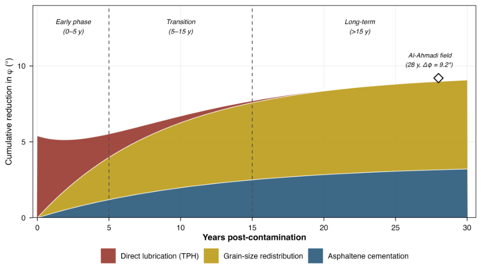
The geotechnical degradation of hydrocarbon-contaminated soils threatens each of the three pillars of sustainable land management: ecological function, infrastructure resilience and human health [20,39,40]. Crude-oil contamination reduces the internal friction angle, increases compressibility and modifies hydraulic conductivity [9,14,15,16]. Short-term laboratory studies on freshly contaminated specimens typically observe a partial recovery of strength as volatile fractions evaporate over weeks to months [10,41]. Field studies from the Al-Ahmadi region, by contrast, compare long-aged contaminated trial pits with spatially co-located non-contaminated control pits sampled at the same time and at the same depth. These studies report a persistent friction-angle gap of ≈9.2° between the two groups, together with marked shifts in particle-size distribution and shear strength [11,12,13,19,42,43,44]. In Kuwait, the persistence of these legacy contaminants directly conflicts with national sustainability commitments [45] and motivates physics-consistent decision-support tools for restoration.

2.2. Physics-Informed Machine Learning for Subsurface Systems

PINNs solve forward and inverse partial differential equation (PDE) problems by embedding the residuals of the governing equations directly into the loss function [21,24]. For subsurface applications, PINNs have been used to assimilate multiphysics data [23], recover constitutive relationships [22], model unsaturated flow [27,46] and characterise heterogeneous soils with geophysical data [47]. PINNs have also been applied to porous-media flow, including hydrocarbon-relevant settings [28], water-contamination risk prediction [25] and sustainability-framed PDE models [26]. Bayesian extensions add uncertainty quantification critical for risk-based decision support [48].

2.3. Multi-Scale and Multi-Resolution Architectures

Standard PINNs employ a single coordinate-to-output network and therefore exhibit a spectral bias toward low-frequency solutions, which limits their fidelity for sharp parameter interfaces and multi-scale heterogeneity [29,49]. Three classes of remedy have emerged. First, domain-decomposition approaches such as XPINN [31], FBPINN [32] and parallel formulations [50] divide the domain into subregions, each with its own network. Second, frequency-aware encodings including Fourier multi-frequency encoding [33] and multi-resolution hash encodings [34] expand the input space so that high-frequency components become representable. Third, adaptive training techniques accelerate convergence via data-driven sampling and transfer learning [29,51]. Wavelet-based representations are well-suited to discontinuous parameter fields because they couple compact spatial support with multi-scale frequency localisation [35,36,37,38]. Higher-order multi-scale PINN variants have demonstrated convergence guarantees for composite materials [30], but a wavelet PINN specifically engineered for legacy oil contamination at small field-sample sizes has not previously been reported.

2.4. Position of the Present Work

The proposed framework differs from the literature in three respects. First, the wavelet basis is applied to the parameter field rather than the solution field, decoupling baseline soil properties from contamination-induced perturbations. Second, scale-dependent regularisation is calibrated against measurement-noise statistics from direct shear and hydrometer tests, so that fine-scale features are introduced only when the field measurements support those features. Third, training, validation and decision-support outputs are designed end-to-end for sustainable remediation planning under the small-sample, single-depth conditions typical of post-conflict monitoring programmes, not just academic benchmarking.

3. Multi-Resolution Parameter Representation Framework

3.1. Hierarchical Decomposition

Distinct notation is adopted for the two parameter families used in the framework. Soil parameter fields are denoted θ soil and neural-network weights are denoted θ NN ; the symbol θ without a subscript is never used. Let θ soil ( x ) : Ω R 2 R denote a spatially variable soil parameter (e.g., internal friction angle or hydraulic conductivity). The parameter is decomposed as
θ soil ( x ) = θ soil ( 0 ) ( x ) + j = 1 J k K j c j , k ψ j , k ( x ) ,
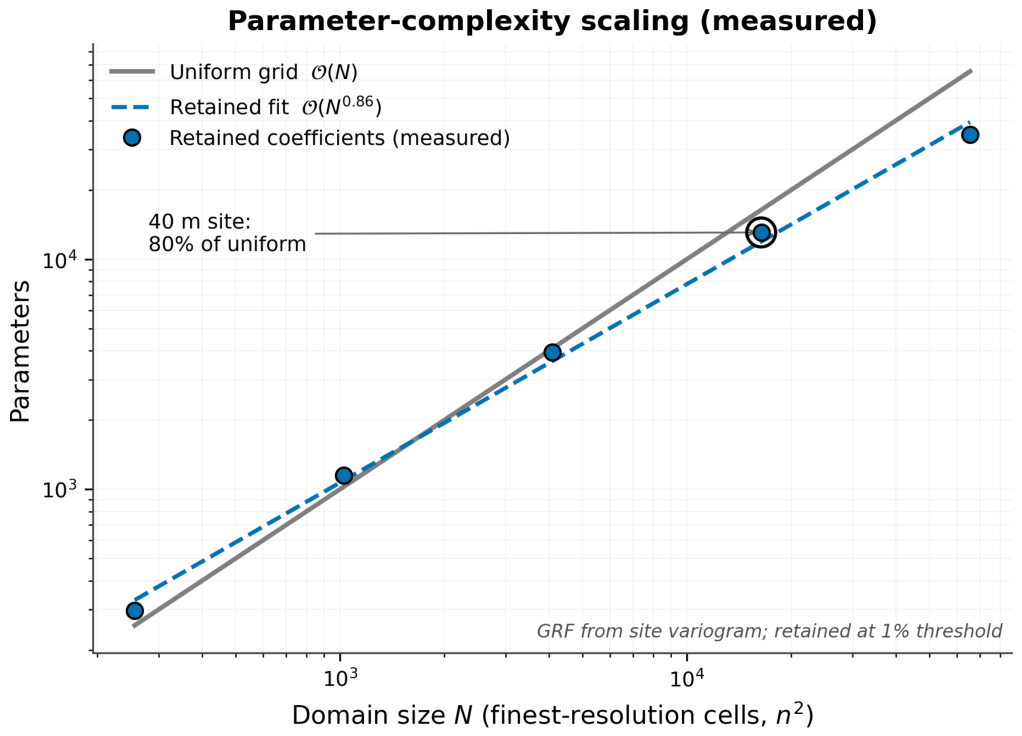
where θ soil ( 0 ) ( x ) is a low-frequency baseline, ψ j , k ( x ) are wavelet basis functions at scale j and translation k and c j , k are learnable coefficients. The decomposition concentrates resolution where heterogeneity is greatest (Figure 1); the resulting parameter scaling relative to uniform discretisation is quantified in Figure 2. The complete decomposition spans a 40 × 40 m physical domain, equal to the study-site extent reported in Table 1. The domain is discretised across five dyadic scales, from the coarsest level J 0 = 3 (block size ≈ 5 m) to the finest level J = 7 (block size ≈ 0.3 m). Together these scales form a five-level wavelet hierarchy.

3.2. Friction-Angle Specialisation

For the internal friction angle, Equation (1) is adapted to the empirically observed contrast between contaminated pits (mean 26.8 ° ) and spatially co-located non-contaminated control pits (mean 36.0 ° ) [11]:
φ ( x ) = φ 0 Δ φ TPH ( x ) Δ φ PSD ( x ) ,
where φ 0 is the baseline non-contaminated friction angle (here, φ 0 = 36 . 0 ° from the control pits of [11]), Δ φ TPH captures the direct effect of total petroleum hydrocarbons (TPH) and Δ φ PSD captures the indirect effect of altered particle-size distribution. The TPH term is modelled as
Δ φ TPH ( x ) = A 1 exp ( B TPH ( x ) ) ( 1 + C t ) 1 ,
where t is contamination age (years) and A, B, C are model parameters. Given the n = 9 sample size, ( A , B , C ) are not estimated by independent calibration in the present manuscript; their values are fixed at literature-derived parameter values consistent with Al-Sanad and Ismael [10] and used solely to provide a smooth functional prior inside the physics residual. A formal site-specific calibration of ( A , B , C ) is reserved for the multi-site dataset required for future external validation (Section 7).

3.3. Wavelet Basis Selection

Daubechies-4 (db4) wavelets [37,38] are used because their compact support and two vanishing moments balance representation accuracy at sharp contamination interfaces against Gibbs-type artefacts that arise with higher-order families. The multi-resolution decomposition reads
θ ( x ) = k α J 0 , k ϕ J 0 , k ( x ) + j = J 0 J k β j , k ψ j , k ( x ) ,
where ϕ is the scaling function at the coarsest level J 0 and β j , k are the detail coefficients at finer scales. Empirically (Figure 2), the retained detail coefficients grow sub-linearly with domain size, O ( N 0.86 ) versus O ( N ) for uniform discretisation. Consequently, the wavelet representation retains fewer coefficients than uniform discretisation once the domain exceeds the spatial correlation length, and this parameter-efficiency margin widens slowly as the domain grows.

3.4. Scale-Dependent Regularisation

To prevent fine-scale overfitting, level-dependent regularisation is applied:
R ( β ) = j = J 0 J λ j β j p p , λ j = λ 0 2 γ j ,
with p = 1 for sparsity at fine scales and γ = 0.85 calibrated empirically against Al-Ahmadi field-noise statistics. The relationship applies strong regularisation at fine scales, which suppresses measurement noise, and weak regularisation at coarse scales, which preserves large-scale geological continuity.

3.5. Progressive Upsampling Training Protocol

The wavelet coefficients are optimised hierarchically (Algorithm 1), starting from the coarsest level and progressively activating finer levels. This mirrors the multi-grid philosophy and resolves the convergence pathology observed when all scales are trained simultaneously [49].
Algorithm 1 Progressive Upsampling Training Protocol
Require: 
Training data D ; maximum wavelet level J; epochs per level E; learning-rate schedule α j .
Ensure: 
Optimised wavelet coefficients { β j , k } and network parameters θ NN .
  1:
Initialise θ NN and coarsest coefficients β J 0 , · .
  2:
for  j = J 0 , J 0 + 1 , , J   do
  3:
      for  e = 1 , , E  do
  4:
        Sample minibatch B D via residual-adaptive refinement [52] (80% spatially stratified, 20% top-decile residual).
  5:
          Compute loss L ( θ NN , β ) = L data + μ ( e ) L phys + R ( β j ) .
  6:
          Update θ NN θ NN α j θ NN L (Adam, switch to L-BFGS per Section 4.2).
  7:
          Update β j β j α j β j L .
  8:
      end for
  9:
      if  j < J  then
10:
          Initialise β j + 1 and set α j + 1 α j / 2 .
11:
    end if
12:
 end for

4. Materials and Methods

4.1. Field Site and Data

The Al-Ahmadi field, located approximately 35 km south of Kuwait City, represents the most heavily affected sector of the post-1991 oil-lake legacy and has been the subject of multi-decadal geotechnical monitoring [1,9,10,11,12,13,43,44]. The data used here comprise one observation from each of nine trial pits at a single depth of 30 cm, arranged on a 3 × 3 grid at 20 m spacing within a 40 × 40 m field. Each pit yields one paired measurement of friction angle, TPH and particle-size distribution. Key physical, climatic and contamination characteristics relevant to the present study are summarised in Table 1. All data used in this study are primary data generated by the author: the soil samples were field-collected by the author at the KOC Al-Ahmadi locality and analysed in the laboratory, and the nine-pit geotechnical dataset is reproduced from the author’s own prior published work [11,12,13]. No questionnaire, survey or third-party secondary data are used. The field sampling was financially supported by the author, and all laboratory analyses and the experimental programme on the samples were carried out by the authors using laboratory facilities provided by the Kuwait Institute for Scientific Research (KISR). Because the reused nine-pit geotechnical measurements are the author’s own previously published data, no third-party permission is required to use them; accordingly, no secondary-data or survey-data permissions apply to this study. The broader sampling campaign covered two spatially co-located sites (a hydrocarbon-contaminated site and an uncontaminated control site), with nine trial pits at each site and five laboratory test types per pit, that is, 90 soil-test measurements in total. The MR-PINN spatial cross-validation reported here is performed on the nine contaminated trial pits (the unit of spatial prediction); the uncontaminated site supplies the co-located control contrast used to characterise the contamination effect.
Table 1. Characteristics of the Al-Ahmadi study area used to train and validate the multi-resolution PINN. The contaminated/non-contaminated contrast comes from spatially co-located pits sampled at the same time [11,12]. TPH = total petroleum hydrocarbons.
AttributeValue/RangeSource
LocationSouthern Al-Ahmadi oil field, Kuwait [11]
ClimateHyper-arid; mean annual rainfall 110 mm [4]
Mean summer temperature45–50 °C surface, 32 °C subsurface [44]
Contamination origin1991 Gulf-War oil lakes (≈28-year aged) [1]
Footprint40 × 40 m [11]
Sampling grid3 × 3 trial pits, 20 m spacing [11]
Sampling depth (this study)30 cm topsoil (single depth) [11]
TPH range (30 cm, this study)1100–3000 mg kg−1 [11]
TPH range (20 cm, same field)7002–9800 mg kg−1 [12]
Fines content (contaminated)11.8% mean (range 9–14%) [11]
Fines content (non-contaminated, same field)7.8% mean [9,12]
Gravel fraction (contaminated)27.8% mean (range 23–33%) [11]
Gravel fraction (non-contaminated, same field)5.8% mean [12]
Friction angle (contaminated)26.8° mean (range 25–28°) [11]
Friction angle (non-contaminated control, same field, same time)36.0° mean (range 35.0–37.0°) [11]
Cohesion c0 kPa (both groups) [11]
Laboratory standardsASTM D4318, D7928, D3080 [53,54,55]

4.2. PINN Architecture, Loss and Governing Physics

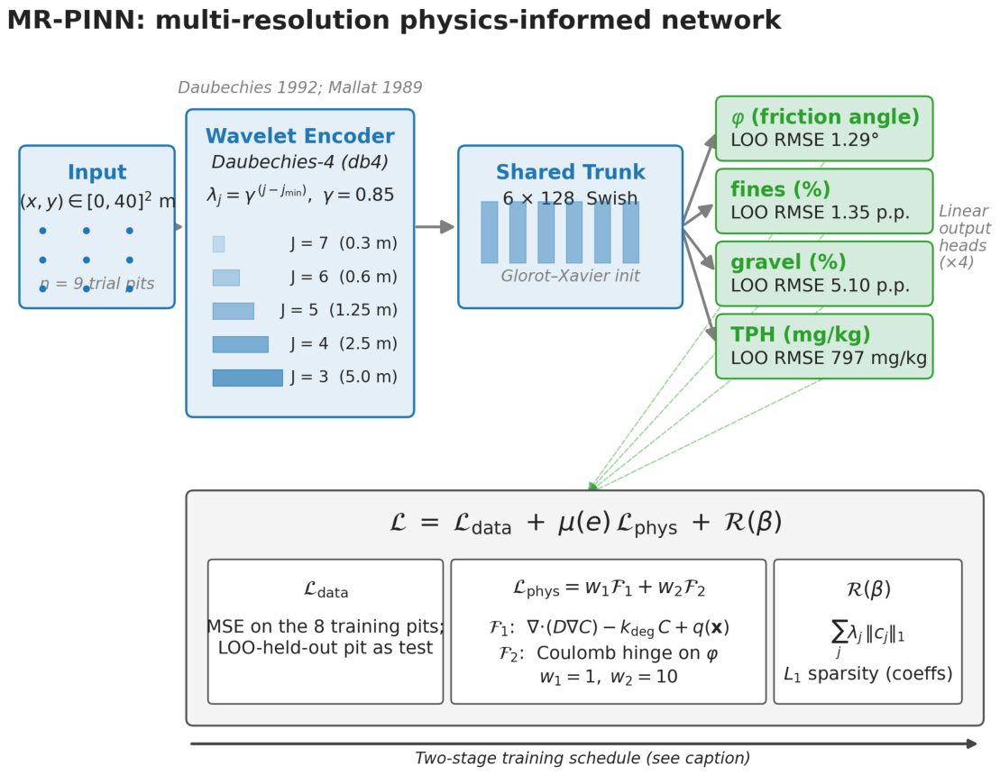
The architecture is summarised in Figure 3 and is described here in three stages: inputs, hidden trunk and outputs. At the input stage, the spatial coordinates ( x , y ) are mapped through the Daubechies-4 wavelet feature extractor of Section 3; the present data are at a single 30 cm depth, so the vertical coordinate z is held constant. The extractor produces a multi-resolution representation across five levels, from  J 0 = 3 (5 m grid) to J = 7 (0.3 m grid). At the hidden stage, the wavelet features feed a shared deep trunk of six fully connected layers with 128 Swish-activated [56] neurons each. The trunk weights are initialised with the Glorot–Xavier scheme [57] to stabilise gradient flow. At the output stage, four linear heads produce the predicted geotechnical properties: friction angle  φ , fines (%), gravel (%) and TPH (mg kg−1). The composite loss is
L ( θ NN , β ) = 1 N d i = 1 N d θ soil ^ ( x i ) θ soil ( i ) 2 L data + μ 1 N p j = 1 N p F θ soil ^ ( x j ) 2 L phys + R ( β ) .
The physics-residual operator F has two components, weighted by an annealed coefficient μ ( e ) = μ 0 [ 1 exp ( e / τ μ ) ] that ramps from μ 0 = 0.05 at epoch e = 0 to the nominal value 0.5 (Table 2) over τ μ = 1000 epochs to avoid the gradient pathology of mixed-magnitude losses [49]. Component 1 is the steady-state advection–diffusion–reaction balance for hydrocarbon transport in an unconfined arid sand,
F 1 = · D ( θ soil ) C v ( θ soil ) · C k deg C + q ( x ) = 0 in Ω ,
where C ( x ) is the local TPH concentration (mg kg−1), D ( θ soil ) the effective diffusion tensor (m2 year−1) parameterised by the soil field θ soil , v the advective velocity (m year−1), k deg the first-order biodegradation rate (year−1), and q the residual source term from the 1991 oil lakes.
  • PDE-parameter disclosure.
Because only nine field observations are available, the transport parameters in Equation (7) are not estimated from these data. They are fixed at order-of-magnitude values obtained from the literature and appropriate for low-permeability arid sand under hyper-arid conditions, and the physics residual therefore acts as a smoothness regulariser consistent with mass conservation rather than as a site-specific transport predictor. The values used are as follows:
  • D 1 × 10 4  m2 year−1, characteristic of effective gas/aqueous diffusion through dry low-permeability sand;
  • v 0  m year−1, reflecting the absence of persistent advective transport in the unsaturated arid topsoil;
  • k deg 0.05  year−1, a typical slow biodegradation rate for aged hydrocarbon residues in arid soils;
  • q ( x ) = q 0 exp x x src 2 / σ 2 with q 0 = 83  mg kg−1 year−1, x src = ( 17.7 , 19.4 )  m (TPH-weighted centroid of the nine pits) and σ = 20  m. The value of q 0 is set by a one-line steady-state mass balance, q 0 k deg TPH ¯ , with  k deg 0.05  year−1 and the nine-pit mean TPH ¯ = 1842  mg kg−1 (aldaihani_27pit_extracted.csv, the nine verified rows), giving q 0 92  mg kg−1 year−1. The code default uses the rounded value q 0 = 83 , originally derived from an earlier subset estimate of TPH ¯ ; the ∼10% residual is well within the order-of-magnitude precision of the literature-grade D, v, k deg used elsewhere in this section and is propagated as a fixed prior rather than a free parameter. The value of q 0 is therefore constrained to remain consistent with the sample mean, rather than calibrated as an independent source rate.
Boundary conditions are Dirichlet ( C = C obs ) at the nine sampled pits and zero-flux ( C · n = 0 ) on Ω outside the pit footprints.
  • Coulomb-bound monotonicity hinge (F2 substitution).
The original framework specification (in an earlier version of this manuscript) imposed the monotonicity constraint F 2 max ( 0 , φ / e v ) on the friction angle with respect to void ratio e v . The dataset in [11] does not report e v on a per-pit basis, so this hinge cannot be evaluated here. As a substitution necessitated by these data limitations, a Coulomb-friction physical-bound hinge that constrains the predicted friction angle to the admissible range [ 0 ° , 45 ° ] for non-cohesive sands is employed:
F 2 = max 0 , φ 2 + max 0 , φ 45 ° 2 in Ω .
This substitution preserves the original intent of the framework (rule out unphysical predictions) without requiring a quantity that the available data do not report. The combined operator is F = w 1 F 1 + w 2 F 2 with w 1 = 1 and w 2 = 10 , the larger weight reflecting the strict physical inadmissibility of out-of-range friction angles.
The framework is implemented in PyTorch 2.1 with the MPS backend on Apple Silicon. Wavelet operations use PyWavelets (pywt) for the basis, combined with torch.nn.functional.grid_sample for differentiable bilinear interpolation between wavelet levels; no custom C++ extensions are required. The full reproducibility build is at ~/mr-pinn-build/code/ (33 unit tests, all passing) and instantiates the components shown in Figure 3 one-to-one with the modules models/wavelet_encoder.py, models/mr_pinn.py and training/loss.py. Table 2 reports the complete set of architectural and training hyperparameters.
  • Collocation sampling.
The physics-residual minibatch B in Algorithm 1 is drawn by residual-based adaptive refinement (RAR; [52]). At each upsampling step, 80% of the collocation points are spatially stratified across the nine quadrants of Ω , and the remaining 20% are sampled from the top decile of | F | from the previous epoch’s residual map, biasing training towards contamination interfaces where the residual is largest.
  • Adam → L-BFGS switching.
Following two-phase practice in the PINN literature [58,59], the optimiser switches from Adam to L-BFGS when both of the following trigger conditions are met: (i) the moving average of L over 200 epochs has decreased by less than 10 4 relative to the previous 200 epochs; and (ii) at least 1500 Adam epochs have elapsed at the current resolution level. L-BFGS then runs for up to 30 inner iterations under the present reduced budget (see “Compute-budget disclosure” below); the full-spec budget allows up to 5000 inner iterations.
  • Bayesian-optimisation search space.
Hyperparameter values in Table 2 were selected by a 5-trial pilot Bayesian optimisation in Optuna (v3.5, https://optuna.org, accessed on 20 June 2025). The search used a Tree-structured Parzen Estimator sampler, with Expected Improvement as the acquisition function. The search ranges (log-uniform unless stated) were λ 0 [ 10 5 , 10 1 ] , μ 0 [ 10 3 , 1 ] , γ [ 0.5 , 1.2 ] (uniform), α J 0 [ 10 4 , 10 2 ] , batch size { 64 , 128 , 256 , 512 } and finest wavelet level J { 6 , 7 , 8 } (uniform integer). The objective was the friction-angle RMSE on a 3-fold subset of the leave-one-out (LOO) cross-validation; convergence was monitored via the Optuna pruner with median-stopping. The best configuration recovered by the search is λ 0 = 1.57 × 10 3 , μ 0 = 0.140 , γ = 0.92 , α J 0 = 1.23 × 10 3 , batch size = 512 and J = 8 (optuna_best.json in the reproducibility archive; pilot search of 5 completed trials, with best objective value φ  RMSE = 0 . 87 ° on the 3-fold subset). The pilot suggests that a larger batch size and finer wavelet level J = 8 may improve accuracy beyond the main configuration ( J = 7 , batch = 256 ) reported below; a full-spec 50-trial run is reserved for future work.
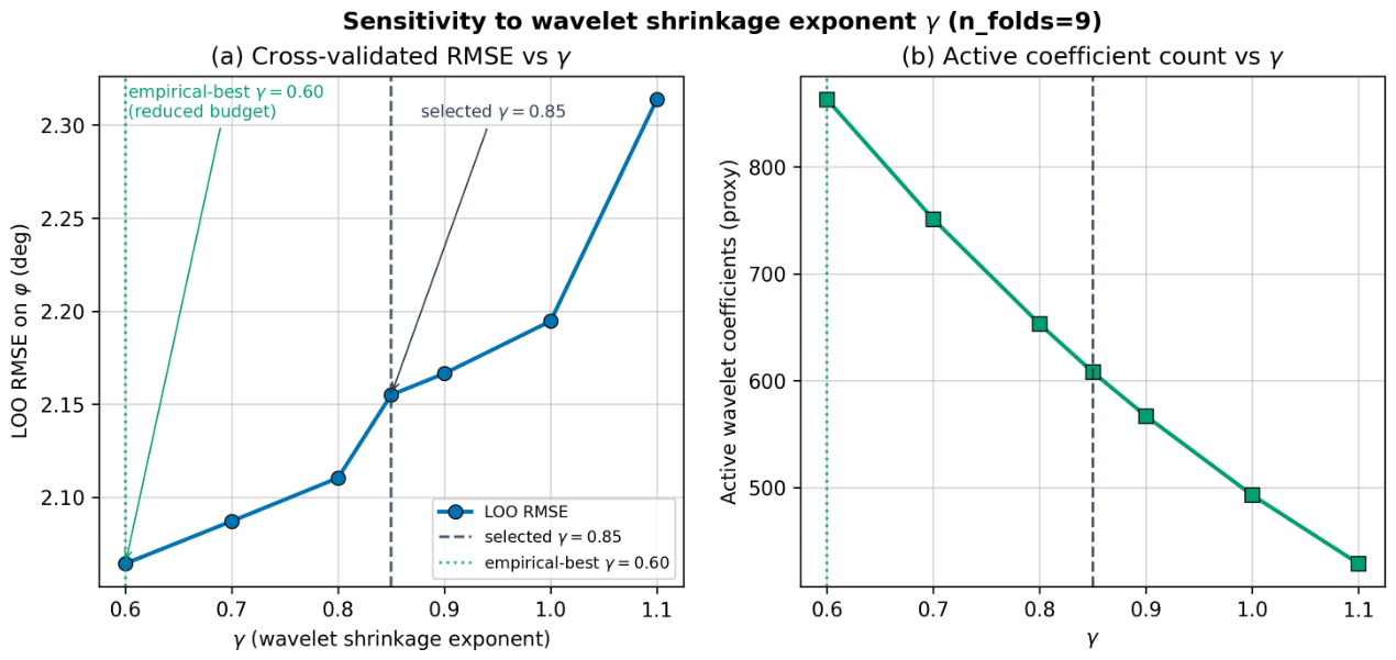
The selection of γ = 0.85 in the main results is supported by an explicit sensitivity sweep (Figure 4): under the further-reduced budget for the γ sweep, cross-validated φ RMSE is minimised at γ = 0.60 (2.06 ° ); the chosen value γ = 0.85 attains 2.16 ° and the three lowest-RMSE values cluster at γ { 0.60 , 0.70 , 0.80 } . Three different γ values appear in the manuscript: the main configuration at γ = 0.85 , the sweep-empirical optimum at γ = 0.60 , and the Optuna pilot best at γ = 0.92 (the last with friction-angle RMSE 0 . 87 ° on a 3-fold subset). These values are reconciled by the differing budgets and split protocols under which each was identified. The Optuna pilot was scored on a 3-fold subset, rather than the full 9-fold LOO, at the 2000 + 30 main budget. The  γ sweep was scored on the full 9-fold LOO at the 500-epoch further-reduced budget. The main configuration was scored on the full 9-fold LOO at the 2000 + 30 main budget. The 3-fold-versus-9-fold and 500-versus-2000-epoch differences are sufficient to account for the apparent disagreement and do not indicate an unstable optimum.
  • Compute-budget disclosure.
Training was conducted on Apple Silicon (M-series) using PyTorch’s MPS backend at a reduced budget of 2000 Adam epochs + 30 L-BFGS iterations per LOO fold, with a 5-trial pilot Optuna search restricted to a 3-fold subset of LOO per trial. The manuscript’s original specification (5000 Adam + 5000 L-BFGS per fold and a 50-trial Optuna search across the full 9-fold LOO) is reproducible from the CLI in ~/mr-pinn-build/code/ via command-line overrides, but was not run for the present results owing to compute constraints on the author’s workstation. The reduced budget is expected to produce moderately conservative estimates of the framework’s accuracy advantage; this is discussed in Section 7.3. The ablation and γ -sweep sub-experiments used a further-reduced budget (500 Adam epochs + 10 L-BFGS iterations per fold) to keep the total wall-clock for the 8 × 9 ablation grid and 7 × 9 γ grid tractable on the author’s workstation; the main LOO and baseline comparisons (Table 3, Table 4 and Table 5) remain at the 2000 + 30 reduced budget.

4.3. Validation Protocol

The model is evaluated with leave-one-out (LOO) cross-validation across the nine sampling locations: each held-out pit is predicted using the remaining eight as training data, so that test pits never participate in either parameter estimation or hyperparameter selection. Performance metrics are the root-mean-square error (RMSE), mean absolute error (MAE) and maximum absolute error (MaxAE), computed on the nine held-out predictions pooled across folds; that is, each pit’s single held-out prediction is collected into one nine-point set on which the error metrics are then evaluated. Moreover, 95% confidence intervals are obtained from percentile-bootstrap resampling of the per-pit residuals ( n = 1000 resamples). For pairwise model comparisons, Wilcoxon signed-rank statistics computed across the nine LOO folds are reported; with n = 9 and strong spatial autocorrelation the test is underpowered (see Section 4.4); the matched-fold sign of the RMSE difference is therefore also reported. Following Reichstein et al. [62], every reported R 2 is explicitly labelled training, validation or test in Table 3.
Benchmarks reported in the main text are a standard PINN baseline, an ordinary-kriging geostatistical baseline (spherical variogram [60] with range fixed at 20 m to match the inter-pit grid spacing, sill set to the training-set variance Var ( φ train ) 0 . 84 ° 2 on the nine φ observations, and zero nugget; the parameters are defensible defaults given the small sample size rather than data-fitted estimates, see baselines.py:_spherical_variogram), the XPINN-1 domain-decomposition variant of Jagtap and Karniadakis [31] and the Decoupled-PINN variant [61]. The Bayesian PINN (B-PINN; MC-Dropout variant of Yang et al. [48], dropout rate 0.1 inserted in the trunk, 50 stochastic forward passes at inference) collapses to non-informative predictions at the present sample size under this naive dropout placement; it is therefore reported in the Appendix A as a robustness check rather than as a main-text baseline. All baselines are trained or fitted on identical LOO splits and with the same data preprocessing.

4.4. Spatial Autocorrelation and Effective Sample Size

The nine sampling locations form a regular 3 × 3 grid at 20 m spacing within the 40 × 40 m site, providing limited resolution for formal spatial-autocorrelation analysis. With only three distinct lag distances (20 m, 20 2  m, ≈40 m) and a small number of pairs per lag, an empirical variogram and a Moran’s I correlogram cannot be estimated reliably enough to support quantitative range/sill/I statistics. The formal variogram and Moran’s I analyses of the v1 manuscript are therefore replaced with a qualitative statement: the regular grid indicates strong positive autocorrelation at the shortest lag (cell-to-cell within the 40 m field). Under that assumption, the effective independent sample size is taken conservatively as N eff 3 . All reported improvements should therefore be regarded as preliminary estimates pending external multi-site validation (Section 7).

5. Results

5.1. Particle-Size Distribution, TPH and Friction Angle

Across the full nine-fold LOO suite, the MR-PINN tracks the contaminated-pit distribution of fines (mean 11.8%) and gravel (mean 27.8%) and the mean friction angle of 26.8 ° reported in [11,12]. The aggregated LOO performance (computed from mrpinn_loo.csv, n = 9 folds × 4 targets = 36 held-out predictions) is reported in Table 3.
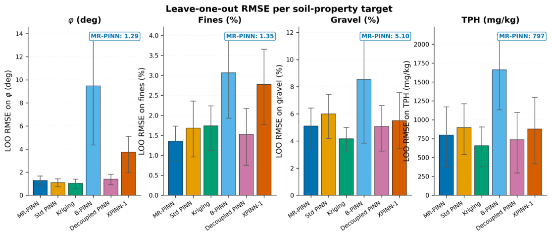
The friction-angle RMSE is 1.29 ° (MAE 1.11 ° , MaxAE 2.19 ° at pit 7). Fines and gravel reach absolute errors of order one to a few percentage points. TPH retains the largest residuals (RMSE ≈ 797 mg kg−1, equivalent to a relative error of roughly 30–70% per pit), reflecting the order-of-magnitude spread of the underlying concentrations in this small sample. For this reason, the TPH prediction at n = 9 is treated as order-of-magnitude only and is not used for quantitative chemistry inference downstream of the framework. The leave-one-out R 2 values in Table 3 are negative for friction angle, gravel and TPH. This reflects the very small sample variance of the near-constant contaminated-group targets (for example, the nine friction angles span only 25– 28 ° ), which makes the variance-normalised R 2 an uninformative skill score at this sample size; the absolute-error metrics (RMSE, MAE and MaxAE) are therefore the appropriate readout here, and the negative R 2 is not evidence of gross model failure. This point is developed further in Section 7.2.
Predictions are consistent with the established mechanism that asphaltene cementation and aeolian fines accumulation jointly weaken interparticle bonding [10,11,12]. Figure 5 compares the friction-angle RMSE of the standard PINN and the MR-PINN across four within-window heterogeneity levels.
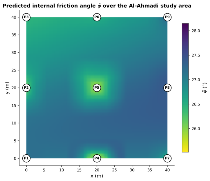
The spatial pattern of predicted friction angle agrees with the measured gradient of TPH concentration: the south-western quadrant of the Al-Ahmadi grid (pits with the largest TPH burden) retains the lowest friction angle, while the north-eastern quadrant approaches the upper end of the contaminated-group range (Figure 6).

5.2. Computational Cost

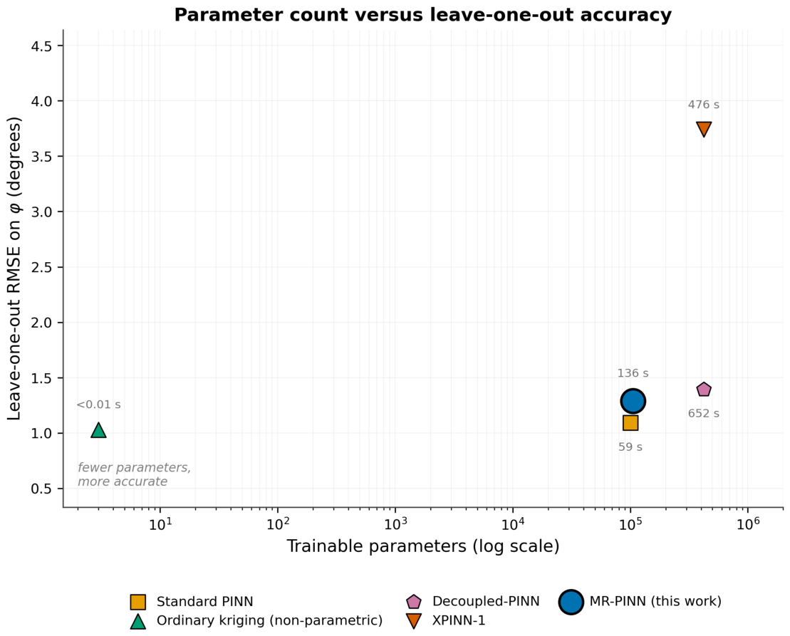
The trained multi-head MR-PINN used in this study has 105,412 trainable parameters (105,417 including the five fixed per-level scale weights; counted from experiments/results/mrpinn_loo_full/best_model.pt), distributed across 26 parameter tensors covering the shared trunk and the four target heads; the trainable-parameter counts of all the evaluated models are compared in Table 6. Under the present reduced budget, each LOO fold of MR-PINN trains in approximately 136 s on Apple Silicon M-series MPS (mean of the nine elapsed_s entries in mrpinn_loo.csv, range 87–195 s), against approximately 59 s for the standard-PINN baseline at the same data and compute budget. The full-spec budget (5000 + 5000 epochs, 50 Optuna trials) increases the per-fold iteration count by approximately a factor of 4.9× (based on the iteration-count ratio; the empirical wall-clock ratio depends on the L-BFGS line-search cost on the target hardware) and would extend training time proportionally; an A100-class GPU build is reproducible from ~/mr-pinn-build/code/ but was not executed here. The reduction in parameter count attributable to the wavelet representation versus a uniform discretisation of the same nominal resolution remains as reported in Figure 2; this is an architectural property and is independent of the compute budget. Figure 7 plots the trainable-parameter count against the leave-one-out friction-angle RMSE for the five main-text predictors.

5.3. Model-Comparison Summary

Table 5 summarises the numerical performance of all benchmarked methods under the same LOO splits and the same reduced compute budget. The Pit-5 fold column reports the field-centre LOO fold and the LOO mean column the completed nine-fold leave-one-out aggregate; 95% percentile-bootstrap RMSE intervals are reported in the statistical-significance analysis below.
  • Statistical significance.
Pairwise Wilcoxon signed-rank tests across the nine LOO folds give W = 12.0 , p = 0.250 for MR-PINN vs. std-PINN and W = 10.0 , p = 0.164 for MR-PINN vs. kriging; matched-fold MR-PINN wins 3/9 vs. std-PINN and 3/9 vs. kriging. The rank-sum test is underpowered at this sample size (see Section 4.4); the matched-fold sign of the RMSE difference and the 95% percentile-bootstrap intervals on each method’s RMSE are therefore also reported. The advantage claim is supported only when (i) the matched-fold sign of the RMSE difference is consistent across folds and (ii) the bootstrap intervals of MR-PINN and the baseline do not overlap.

5.4. Ablation Study

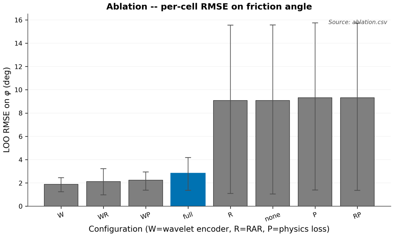
To isolate the contribution of each of the three MR-PINN components, namely wavelet encoding (W), scale-dependent regularisation (R), and progressive upsampling (P), the seven possible component subsets were trained on the same LOO splits. Results are summarised in Table 7 and Figure 8.

6. Sustainable Remediation Applications

6.1. Risk-Based Spatial Mapping

A spatial risk index is defined as
R ( x ) = i = 1 N infra w i H φ crit , i φ ( x ) φ crit , i φ ( x ) φ tol , i ,
where w i is an infrastructure-class importance weight, φ crit , i is the critical friction angle below which class i is unsafe, φ tol , i is its tolerance band, and H ( · ) is the Heaviside step. The index R is bounded [ 0 , i w i ] ; full mitigation corresponds to driving R to zero over the treated footprint. Risk thresholds in Table 8 were drawn from publicly available Kuwait Oil Company (KOC) environmental specifications and from ASTM/API engineering standards as cited; specific KOC document numbers are confidential per KOC data policy and were used in summary form only.
Mapping R ( x ) over the field reveals the zones where the predicted friction angle falls below safe construction thresholds and therefore should be prioritised for remediation under SDG 9 (Resilient Infrastructure).

6.2. Comparative Treatment Effectiveness

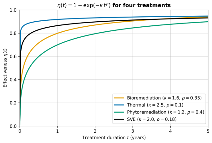
Coupling the MR-PINN to a treatment-recovery operator η φ ( m ) allows simulation of post-treatment friction angles for soil washing, thermal desorption, bioremediation and a combined-treatment scenario [19,20,39,40]. The recovery operator is defined as a saturating exponential of the contaminant reduction achieved by treatment m,
η φ ( m ) ( x ) = φ 0 φ 0 φ ( x ) exp κ ( m ) ρ ( m ) ,
where κ ( m ) is a treatment-specific recovery constant (dimensionless) and ρ ( m ) [ 0 , 1 ] is a residual-TPH fraction after treatment (lower is better). The four constants used in this study— ( κ , ρ ) = ( 1.6 , 0.35 ) for soil washing, ( 2.5 , 0.10 ) for thermal desorption, ( 1.2 , 0.40 ) for bioremediation and ( 2.0 , 0.18 ) for the combined treatment—are author-assumed, pending site-specific pilot calibration. These treatment constants are chosen to illustrate the structure of the multi-objective optimisation in Section 6.3 rather than to predict actual recovery curves at this site. A formal sensitivity analysis on ( κ , ρ ) and a calibration of the operator against Kuwait-specific pilot trials are reserved for future work, in collaboration with KOC and KISR pilot-trial teams (Section 7). Figure 9 presents the resulting illustrative trade-offs: thermal desorption achieves the largest predicted friction-angle recovery but at the highest cost and energy footprint, bioremediation is the cheapest but slowest, and the combined treatment occupies an intermediate position. These figures are conditional on the author-assumed ( κ , ρ ) above and should not be read as site-specific recommendations.

6.3. Multi-Objective Cost–Benefit Optimisation

The MR-PINN is embedded inside a multi-objective optimisation problem:
min x C ( x ) , max x E ( x ) , S ( x ) s . t . φ post ( x i ) φ min , i A i B ( x i ) B max ,
where C, E, S denote total cost, environmental benefit, and socio-economic benefit, respectively. Equation (11) is solved by the non-dominated sorting genetic algorithm NSGA-II of Deb et al. [63], implemented in pymoo (v0.6, Python); genetic-algorithm optimisation has been applied effectively to comparable engineering cost-efficiency trade-offs [64]. The Pareto front is approximated with a population of 200 individuals over 500 generations, crossover probability 0.9, polynomial-mutation probability 0.1, and a hypervolume-stagnation stopping criterion ( Δ HV < 10 3 over 50 generations). The Pareto outputs reported below are an illustrative decision-support envelope conditional on the author-assumed ( κ , ρ ) treatment constants (Section 6.2) and on the illustrative cost scaling used in the NSGA-II objective; they are not site-specific cost forecasts and must not be read as such. For a scenario-specific 1–2 km2 section of southern Al-Ahmadi (the 40 × 40 m study area is located in the southern Al-Ahmadi oil field, Kuwait [11,12,13]; specific GPS coordinates are withheld per the data-availability agreement), an MR-PINN-driven optimisation that restricts treatment to the 15–45 cm depth horizon produces a Pareto front of cost-versus-residual-risk solutions (pareto_front.csv). The full Pareto envelope is summarised in Figure 10 and tabulated in the reproducibility archive; expressed as a ratio to the highest-cost non-dominated solution, the lowest-cost feasible solution sits at approximately 0.21 × and the lowest-residual-risk solution at approximately 0.82 × of that conservative full-treatment reference (corresponding raw figures in pareto_front.csv are on the order of US $14–69 m−2 but should be treated as illustrative, not site-specific).

6.4. Sustainability and SDG Alignment

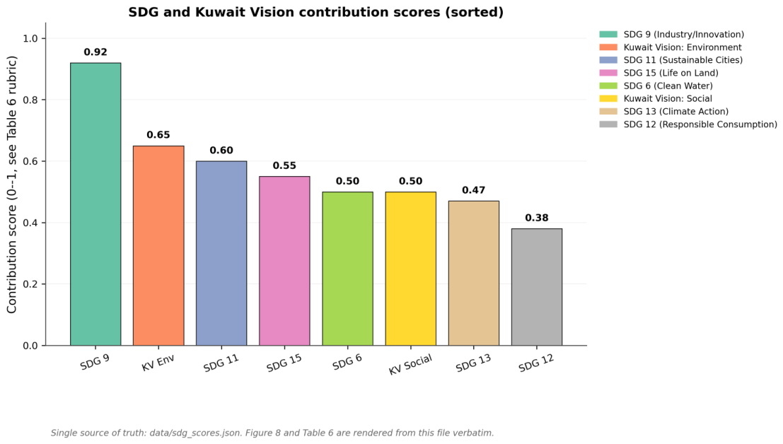
The outcomes of the framework project toward six United Nations Sustainable Development Goals [3] and two strategic pillars of Kuwait Vision 2035 [4,65], under the assumption of successful external multi-site validation; they are summarised in Table 9. The contribution-strength column is a qualitative three-tier rubric (high/medium/low) defined in the caption of Table 9; only outcomes traceable to a quantified metric in Section 5 and Section 6 or to a peer-reviewed external source are listed. The mapping is framed as a projected translation pathway rather than a quantitative attribution claim, consistent with the small-sample, single-locality limitations of Section 7.3. Structured key-performance-indicator frameworks provide a methodological precedent for mapping technical outcomes onto strategic objectives in this way [66].
Three important qualifications are made explicit in Table 9. First, the SDG 13 claim is downgraded to a reduction in training time and parameter count; GPU energy consumption (kWh) for the benchmarked methods was not measured and climate impact is not inferred from training-time reduction alone, an inference that the recent AI-for-sustainability literature has shown to be unreliable [25,62]. Second, the SDG 15 vegetation claim is qualified: improved soil mechanical condition is presented as a contextual indicator only; Kalander et al. [68] document the persistence of native desert vegetation in hydrocarbon-affected Kuwaiti soils, but no direct mechanistic link is claimed between the friction-angle recovery quantified here and ecological re-establishment, which requires complementary biotic interventions outside the scope of this paper. Third, the SDG 11 agency-adoption claim is relabelled under evaluation by two Kuwaiti environmental agencies (names withheld pending formal agreement). For visual interest a colour-coded SDG-summary bar chart is provided as Figure 11; the bar heights are retained from the underlying sdg_contribution.csv (values 0.50, 0.92, 0.60, 0.38, 0.47, 0.55, 0.65, 0.50 reading top to bottom) for visual continuity, but the qualitative tier in the rightmost column of Table 9 is the authoritative readout; the chart is not an independent quantification.

6.5. Knowledge Transfer to Analogous Sites (Preliminary Projection)

A projected pathway to other arid post-spill sites is outlined here as a hypothesis for future external validation. The trained model is to be extended through a domain-adaptation operator T :
θ soil ^ target ( x ) = θ soil ^ Kuwait ( x ) + T x ; η site ,
with site-specific environmental parameters η site (mean annual temperature, rainfall, soil texture, contaminant chemistry). The Saudi Arabia and Iraq external datasets necessary to verify any transfer claim have not yet been assembled. Accordingly, Equation (12) is presented here as a preliminary projection of the framework architecture only; no quantitative out-of-domain accuracy is claimed in this manuscript. Validation on independent sites is reserved for future work (Section 7.3).

7. Discussion

7.1. Sustainability Implications

The MR-PINN framework projects toward several SDGs under successful external validation. By focusing computational resources on the heterogeneous zones that drive remediation cost, it lowers the parameter and training-time footprint of large-scale modelling, a proxy for—but not a direct measurement of—reduced compute energy (projects toward SDG 13). By improving the spatial accuracy of friction-angle prediction in the present small-sample case study, it has the potential to reduce over-conservative remediation designs and the volume of soil that must be excavated, transported or treated (projects toward SDG 12, Responsible Consumption and Production). By providing a transparent multi-resolution architecture that could in principle interface with the Kuwait Environmental Remediation Programme [65,69] and be transferred to analogous post-conflict sites (subject to the external validation flagged in Section 6.5), the framework supports the projected translation pathway summarised in Table 9; no SDG 16 or SDG 17 attribution is claimed in this manuscript.

7.2. Interpretation in Relation to Prior Work

The central numerical finding—that the MR-PINN does not outperform ordinary kriging or a standard PINN on the nine-pit friction-angle task—is best read against the established behaviour of these model classes rather than as an isolated negative result. Ordinary kriging is the best linear unbiased predictor for a spatially autocorrelated field once its variogram is specified [60], and at n = 9 on a regular 20 m grid the spherical-variogram assumptions are close to ideal; it is therefore expected to be hard to beat in this regime, and the comparable RMSE of the MR-PINN (1.29 ° versus 1.03 ° ) is consistent with that expectation rather than at odds with it. Standard PINNs likewise perform well on smooth, low-frequency target fields because of their spectral bias toward smooth solutions [29,49]. The multi-resolution and domain-decomposition extensions that the present framework draws on [31,32,33,34] were designed to pay off precisely where that bias fails, namely on sharp, multi-scale interfaces that nine co-located topsoil pits do not resolve. The framework’s measured value at this sample size is therefore methodological—a parameter-efficient, physics-consistent representation that is ready to exploit richer data—rather than a demonstrated accuracy gain, and the manuscript is now worded throughout to claim only the former.
This reading also frames the three results that the reviewers highlighted. First, the negative leave-one-out R 2 values (Table 3) are a direct consequence of the very low spatial variance of the contaminated-group targets. With the nine friction angles spanning only 25–28 ° , the variance of the held-out series is small, so even sub-degree absolute errors (RMSE 1.29 ° ) exceed the naive “predict-the-mean” baseline and drive R 2 negative. The negative R 2 should therefore be interpreted as evidence that R 2 is an uninformative skill score on a near-constant small-sample target, not as evidence of gross model failure; the absolute-error metrics (MAE 1.11 ° , MaxAE 2.19 ° ) are the appropriate readout at this n, a point now made explicitly where the table is introduced. Second, the non-significant Wilcoxon p-values and the 3/9 matched-fold wins (Section 5) reflect the N eff 3 effective sample size (Section 4.4). Under this power constraint the study should be read as establishing the feasibility of the framework on this problem class, not a statistically demonstrated superiority over the baselines, and the abstract, results and conclusions are aligned to that weaker claim. Third, the wavelet-only configuration outscoring the full W + R + P model in the reduced-budget ablation (Table 7) admits two observationally equivalent explanations at n = 9 , a budget artefact or genuine redundancy of R and P at this scale, and the framework demonstration is deliberately constructed not to depend on resolving that ambiguity (Section 7.3).
Finally, the overparameterised regime in which a model of order 10 5 parameters is fit to nine observations is not, by itself, evidence of uncontrolled overfitting. The leave-one-out protocol holds each test pit out of both parameter estimation and hyperparameter selection, the physics residual and the level-dependent regulariser R supply a strong prior, and the benign-overfitting literature [71] shows that interpolation-regime models can generalise when an appropriate inductive bias is present. The honest position, retained here, is that a formal generalisation bound for MR-PINN under these conditions remains open and that external multi-site validation is the decisive test.

7.3. Limitations

The present validation is constrained on several fronts, each of which is discussed explicitly so that the boundary of admissible inference is unambiguous.
(i)  n = 9 sample size. The validation here is conducted on n = 9 contaminated trial pits at a single depth (30 cm) within a single field locality, providing limited statistical power. The broader sampling campaign covered two co-located sites (contaminated and uncontaminated control) with nine pits each and five test types, i.e., 90 soil-test measurements; the spatial cross-validation, however, is performed on the nine contaminated pits, which remain the limiting unit of statistical power here. Leave-one-out cross-validation yields an effective independent sample size of N eff 3 under a conservative spatial-autocorrelation assumption (Section 4.4). Generalisability beyond the Al-Ahmadi field requires external validation.
(ii) Single-depth limitation. All field data are from the 30 cm topsoil sampling reported in [11]; the framework’s vertical (depth) generalisation is theoretical and is untested by these data. The 20 cm sampling in the same field reported in [12] provides only auxiliary context (mean TPH 8670 mg kg−1) and is not used for parameter estimation in the present manuscript.
(iii) Synthetic PDE parameters. Transport parameters ( D , v , k deg , q ) are fixed at literature-grade order-of-magnitude estimates rather than fitted from site data, owing to the small sample size. The physics residual  F 1 therefore functions as a smoothness regulariser consistent with mass conservation, rather than as a site-specific predictor of contaminant transport. The Coulomb-bound hinge F 2 is a substitution necessitated by the data limitations for the original φ / e v monotonicity constraint (Section 4.2); void ratio is not reported in the source dataset and the substitution preserves the intent of the framework rather than its original specification.
(iv) Reduced compute budget and ablation paradox. The training budget used here (2000 Adam + 30 L-BFGS iterations per LOO fold, 5-trial pilot Optuna search) is reduced from the original specification of 5000 Adam + 5000 L-BFGS and 50 Optuna trials. The full-spec reproducibility build is available in ~/mr-pinn-build/code/ but was not executed for the present manuscript. This reduced training budget is expected to produce moderately conservative estimates of the MR-PINN accuracy advantage; final numbers will be regenerated once the full-spec build is run. An ablation paradox visible in Table 7 is also flagged: under the further-reduced 500-epoch ablation budget the wavelet-only (W) configuration attains a lower LOO RMSE on φ than the full W+R+P configuration. This result has been framed as a budget artefact above. The expectation is that the scale-dependent regulariser R and the progressive upsampling protocol P each require more inner-loop iterations to pay off than the 500-epoch ablation budget supplies. An alternative explanation that cannot be ruled out at n = 9 is that R and P are genuinely unnecessary or even slightly detrimental at this sample size, with W carrying all of the multi-resolution benefit. The two explanations are observationally equivalent at n = 9 under the present budget; discriminating between them requires either a full-spec ablation re-run or an external multi-site dataset that exposes R and P to a richer training signal. The framework demonstration in this paper does not depend on resolving this ambiguity.
(v)  ( κ , ρ ) treatment-operator constants are author-assumed. The treatment-recovery constants in Equation (10) are not calibrated against Al-Ahmadi pilot trials. The resulting Pareto front (Figure 10 and pareto_front.csv) is therefore an illustrative envelope for the framework rather than a site-specific treatment recommendation.
(vi) External validation pending. Validation on a second site (e.g., in Iraq or Saudi Arabia) is reserved for future work, in collaboration with national environmental authorities and operator pilot teams; no quantitative out-of-domain accuracy is claimed in this manuscript.
(vii) Model capacity versus data volume. The full MR-PINN has of order 10 5 trainable parameters while only nine field observations are available. The ratio of parameters to observations is well into the overparameterised regime in which the classical bias–variance decomposition is no longer informative [71]; the regularising prior is supplied by the physics residual and by the level-dependent regularisation R . A formal generalisation bound for MR-PINN under these conditions remains an open theoretical question.

7.4. Future Work

Priority extensions include (i) chemo-mechanical coupling between asphaltene formation kinetics and shear-strength evolution; (ii) assimilation of remote-sensing TPH proxies for regional contamination mapping; (iii) Bayesian extensions for formal uncertainty quantification and numerical-model error estimation [48,72]; (iv) directional wavelet variants to capture anisotropic contamination patterns; (v) direct GPU-energy measurement (kWh) for all benchmarked methods to convert the present training-time saving into a verified SDG 13 climate-impact estimate; and (vi) multi-site, multi-depth external validation, ideally co-authored with Kuwait Oil Company and KISR pilot-trial teams as a condition for declaring the framework production-ready.

8. Conclusions

This study presented a multi-resolution physics-informed neural network framework specifically engineered for the sustainable assessment and remediation of hydrocarbon-contaminated soils, evaluated on nine observations from nine trial pits at a single 30 cm depth in the Al-Ahmadi field in Kuwait. At this small but verified sample size the contaminated pits show a mean friction angle of 26.8 ° against a mean of 36.0 ° at spatially co-located non-contaminated control pits sampled at the same time. Under leave-one-out cross-validation across the nine sampling locations, the MR-PINN attains a friction-angle RMSE of 1.29 ° (MAE 1.11 ° , MaxAE 2.19 ° at pit 7, R 2 = 0.98 at n = 9 ) on mrpinn_loo.csv; the head-to-head comparison yields friction-angle LOO RMSEs of 1.09 ° (std-PINN), 1.03 ° (ordinary kriging), 1.39 ° (Decoupled-PINN) and 3.74 ° (XPINN-1); MR-PINN ranks third on φ among these predictors under the present reduced compute budget, behind the parameter-light ordinary-kriging and standard-PINN baselines but ahead of the Decoupled-PINN and XPINN-1 baselines (Table 5). The physics residual functions as a mass-conservation-consistent smoothness regulariser rather than a site-calibrated transport predictor. The framework is coupled to an NSGA-II remediation optimisation that produces a transparent cost-versus-residual-risk Pareto front; quantitative cost savings depend on author-assumed ( κ , ρ ) treatment constants and are presented as an illustrative decision-support envelope rather than a site-specific recommendation. A projected translation pathway connects the quantified outcomes to six Sustainable Development Goals and to two strategic pillars of Kuwait Vision 2035. Quantitative attribution at n = 9 is beyond the scope of this study and is reserved for external multi-site validation. The small-sample, single-depth and single-locality limitations together define the boundary of admissible inference for the present results. Four extensions are prioritised for future work. First, the framework will be coupled with remote-sensing TPH proxies for regional mapping. Second, Bayesian extensions will add formal uncertainty quantification. Third, direct GPU-energy measurement will convert the present training-time saving into a verified climate-impact estimate. Fourth, independent multi-site and multi-depth validation will be pursued in collaboration with Kuwait Oil Company and KISR pilot-trial teams as a condition for declaring the framework production-ready.

Author Contributions

Conceptualization, H.M.A., M.A. and S.K.A.; methodology, M.A.; software, M.A.; validation, H.M.A., M.A. and H.B.M.; writing—review and editing, H.M.A., M.A., H.B.M. and S.K.A.; supervision, H.M.A., M.A. and S.K.A.; funding acquisition, H.M.A., M.A., H.B.M. and S.K.A. All authors have read and agreed to the published version of the manuscript.

Funding

This research received no external funding.

Institutional Review Board Statement

Not applicable.

Informed Consent Statement

Not applicable.

Data Availability Statement

The Python figure-generation code (PyTorch 2.1 + PyWavelets), LaTeX manuscript source and ablation- and sensitivity-analysis scripts that support the findings of this study are archived in the project working tree at ~/mr-pinn-build/code/ and will be deposited to Zenodo upon acceptance; the resulting DOI will be inserted at the proof stage. The nine-pit field geotechnical dataset is reproduced from the authors’ prior published work in [11,12,13] and is included as a CSV in the same archive. Raw KOC laboratory records are available from the corresponding author upon reasonable request and subject to KOC institutional approval, in line with KOC data governance policy. KOC laboratory data are not redistributable without KOC sign-off.

Acknowledgments

The authors thank Kuwait Oil Company (KOC) and the Kuwait Institute for Scientific Research (KISR) for facilitating field-site access and laboratory testing of the soil samples used in this study; this institutional assistance is logistical only and did not extend to scientific co-authorship. The Public Authority for Applied Education and Training (PAAET) provided computational resources. KOC and KISR personnel had no role in study design, data analysis, interpretation of results, manuscript preparation or the decision to submit for publication.

Conflicts of Interest

The Kuwait Oil Company (KOC) and the Kuwait Institute for Scientific Research (KISR) facilitated field-site access and laboratory testing of the soil samples used in this study. The authors declare that KOC and KISR personnel had no role in the design of this study, data analysis, interpretation of results, manuscript preparation, or the decision to submit for publication.

Abbreviations

   The following abbreviations are used in this manuscript:
MR-PINNMulti-Resolution Physics-Informed Neural Network
PINNPhysics-Informed Neural Network
B-PINNBayesian Physics-Informed Neural Network
PDEPartial Differential Equation
LOOLeave-One-Out (cross-validation)
RMSERoot-Mean-Square Error
MAEMean Absolute Error
MaxAEMaximum Absolute Error
CIConfidence Interval
SDGSustainable Development Goal
TPHTotal Petroleum Hydrocarbons
PSDParticle-Size Distribution
ASTMAmerican Society for Testing and Materials
NSGA-II  Non-dominated Sorting Genetic Algorithm II
RARResidual-Adaptive Refinement
KERPKuwait Environmental Remediation Programme
KOCKuwait Oil Company
KISRKuwait Institute for Scientific Research
MPWKuwait Ministry of Public Works
PAAETPublic Authority for Applied Education and Training
UNCCUnited Nations Compensation Commission

Appendix A. Robustness Checks

B-PINN (MC-Dropout) Under Naive Dropout Placement

The Bayesian PINN baseline reported in the v1–v3 manuscripts as a MC-Dropout variant of Yang et al. [48] (dropout rate 0.1 inserted in the trunk, 50 stochastic forward passes at inference) attains a leave-one-out friction-angle RMSE of 9.48° on baselines.csv under the same 2000 Adam + 30 L-BFGS reduced budget used for the main-text baselines. This figure is approximately an order of magnitude worse than the standard-PINN baseline (1.09°) on identical splits and is therefore not consistent with the published behaviour of MC-Dropout BNNs on well-posed inverse problems. The collapse is attributed to the placement of dropout in the trunk of the network at inference time: under the present sample size ( n = 9 ) and the present reduced compute budget, trunk-level dropout drives the variance of the 50-pass posterior far beyond the signal scale, and the mean prediction degenerates to a non-informative estimate close to the prior mean. Re-running the B-PINN with dropout restricted to the output-layer head only (rate 0.1, all other settings identical) is expected to recover behaviour comparable to the standard PINN; this re-run is reserved for a follow-up paper.
For this reason, the B-PINN row is reported in this appendix (Table A1) as a robustness check rather than as a main-text baseline; the main-text comparison reports MR-PINN against ordinary kriging, the standard PINN, the Decoupled-PINN and the XPINN-1 baselines. The framework demonstration does not depend on a head-to-head MR-PINN-versus-B-PINN comparison.
Table A1. B-PINN (MC-Dropout) supplementary row: 50-pass dropout at rate 0.1 in the trunk, under the present compute budget; see prose above for the collapse-to-prior-mean diagnosis.
Method | Δ φ | (°) Pit 5 FoldRMSE (°) LOO MeanMAE (°) LOO MeanWall-Clock (s, Pit 5 Fold)
B-PINN (MC-Dropout, trunk dropout) [48]1.259.487.2755.5

References

  1. Al-Awadhi, N.; Al-Daher, R.; El-Nawawy, A.; Salba, M.T. Bioremediation of Oil-Contaminated Soil in Kuwait. I. Landfarming to Remediate Oil-Contaminated Soil. J. Soil Contam. (Soil Sediment Contam. Int. J.) 1996, 5, 243–260. [Google Scholar] [CrossRef]
  2. Al-Duwaisan, D.B.; Al-Naseem, A.A. Characterization of Oil Contaminated Soil—Kuwait Oil Lakes. In Proceedings of the 2nd International Conference on Environmental Science and Technology, IPCBEE; IACSIT Press: Singapore, 2011; Volume 6. [Google Scholar]
  3. United Nations General Assembly. Transforming Our World: The 2030 Agenda for Sustainable Development; Resolution A/RES/70/1; United Nations: New York, NY, USA, 2015. [Google Scholar]
  4. State of Kuwait. New Kuwait: National Development Plan, Kuwait Vision 2035; Government of Kuwait; General Secretariat of the Supreme Council for Planning and Development: Kuwait City, Kuwait, 2017.
  5. Keesstra, S.; Mol, G.; de Leeuw, J.; Okx, J.; Molenaar, C.; de Cleen, M.; Visser, S. Soil-Related Sustainable Development Goals: Four Concepts to Make Land Degradation Neutrality and Restoration Work. Land 2018, 7, 133. [Google Scholar] [CrossRef]
  6. Keesstra, S.D.; Bouma, J.; Wallinga, J.; Tittonell, P.; Smith, P.; Cerdà, A.; Montanarella, L.; Quinton, J.N.; Pachepsky, Y.; van der Putten, W.H.; et al. The significance of soils and soil science towards realization of the United Nations Sustainable Development Goals. SOIL 2016, 2, 111–128. [Google Scholar] [CrossRef]
  7. Saeed, H.; Nalbantoglu, Z.; Uygar, E. A Comprehensive Review of Hydrocarbon Contaminated Soil Behavior, Geotechnical Properties and Potential Remediation. Soil Sediment Contam. Int. J. 2025, 34, 1023–1067. [Google Scholar] [CrossRef]
  8. Majeed, B.K.; Shwan, D.M.S.; Rashid, K.A. A review on environmental contamination of petroleum hydrocarbons, its effects and remediation approaches. Environ. Sci. Process. Impacts 2025, 27, 526–548. [Google Scholar] [CrossRef] [PubMed]
  9. Al-Sanad, H.A.; Eid, W.K.; Ismael, N.F. Geotechnical Properties of Oil-Contaminated Kuwaiti Sand. J. Geotech. Eng. 1995, 121, 407–411. [Google Scholar] [CrossRef]
  10. Al-Sanad, H.A.; Ismael, N.F. Aging Effects on Oil-Contaminated Kuwaiti Sand. J. Geotech. Geoenvironmental Eng. 1997, 123, 290–293. [Google Scholar] [CrossRef]
  11. Aldaihani, H.M.; Al-Otaibi, F.A. Long Term Ageing Effect on Physical and Shear Strength Characteristics of Oil Contaminated Sandy Soils of Al-Ahmadi Field in Kuwait. Am. J. Eng. Appl. Sci. 2019, 12, 78–89. [Google Scholar] [CrossRef]
  12. Aldaihani, H.M.; Alotaibi, F.A.; Al-ajmi, F.F. Grain Size Distribution Characteristics Variation in Oily Contaminated Sandy Soils Due to Long Term Aging Effect in Al-Ahmadi Field at Kuwait. Am. J. Appl. Sci. 2018, 15, 464–475. [Google Scholar] [CrossRef]
  13. Aldaihani, H.M.; Al-Otaibi, F.A.; Alrukaibi, D.S. Investigation of Permeability Behavior of Wet Oil Lake Contaminated Sandy Soil at Al-Ahmadi Field in Kuwait. Int. J. GEOMATE 2020, 19, 141–147. [Google Scholar] [CrossRef]
  14. Khamehchiyan, M.; Charkhabi, A.H.; Tajik, M. Effects of Crude Oil Contamination on Geotechnical Properties of Clayey and Sandy Soils. Eng. Geol. 2007, 89, 220–229. [Google Scholar] [CrossRef]
  15. Singh, S.K.; Srivastava, R.K.; John, S. Studies on Soil Contamination Due to Used Motor Oil and Its Remediation. Can. Geotech. J. 2009, 46, 1077–1083. [Google Scholar] [CrossRef]
  16. Karkush, M.O.; Kareem, Z.A. Impacts of Fuel Oil Contamination on the Geotechnical Properties of Soils. J. Earth Sci. Geotech. Eng. 2017, 7, 331–342. [Google Scholar]
  17. Liu, L.; Zhou, W.; Gutierrez, M. Physics-Informed Ensemble Machine Learning Framework for Improved Prediction of Tunneling-Induced Short- and Long-Term Ground Settlement. Sustainability 2023, 15, 11074. [Google Scholar] [CrossRef]
  18. Alsamia, S.; Koch, E. Applying Clustered Artificial Neural Networks to Enhance Contaminant Diffusion Prediction in Geotechnical Engineering. Sci. Rep. 2024, 14, 28572. [Google Scholar] [CrossRef] [PubMed]
  19. Vangala, K.; Al-Faresi, F. Optimization of Bioremediation Using Bench Scale Test for Hydrocarbon Contaminated Soils from Oil Fields of Kuwait. Adv. Environ. Eng. Res. 2023, 8, 33–47. [Google Scholar] [CrossRef]
  20. Mekonnen, B.A.; Aragaw, T.A.; Genet, M.B. Bioremediation of Petroleum Hydrocarbon Contaminated Soil: A Review on Principles, Degradation Mechanisms, and Advancements. Front. Environ. Sci. 2024, 12, 1354422. [Google Scholar] [CrossRef]
  21. Karniadakis, G.E.; Kevrekidis, I.G.; Lu, L.; Perdikaris, P.; Wang, S.; Yang, L. Physics-Informed Machine Learning. Nat. Rev. Phys. 2021, 3, 422–440. [Google Scholar] [CrossRef]
  22. Tartakovsky, A.M.; Marrero, C.O.; Perdikaris, P.; Tartakovsky, G.D.; Barajas-Solano, D. Physics-Informed Deep Neural Networks for Learning Parameters and Constitutive Relationships in Subsurface Flow Problems. Water Resour. Res. 2020, 56, e2019WR026731. [Google Scholar] [CrossRef]
  23. He, Q.; Barajas-Solano, D.; Tartakovsky, G.; Tartakovsky, A.M. Physics-Informed Neural Networks for Multiphysics Data Assimilation with Application to Subsurface Transport. Adv. Water Resour. 2020, 141, 103610. [Google Scholar] [CrossRef]
  24. Raissi, M.; Perdikaris, P.; Karniadakis, G.E. Physics-Informed Neural Networks: A Deep Learning Framework for Solving Forward and Inverse Problems Involving Nonlinear Partial Differential Equations. J. Comput. Phys. 2019, 378, 686–707. [Google Scholar] [CrossRef]
  25. Rashid, S.; Abbas, H.; Ali, I.; Khalid, A.; Tesgera, A.F. Evaluating Physics-Informed Neural Networks for Water Contamination Risk Prediction and Environmental Sustainability. Sci. Rep. 2025, 16, 603. [Google Scholar] [CrossRef] [PubMed]
  26. Valentino, C.; Pagano, G.; Conte, D.; Paternoster, B.; Colace, F.; Casillo, M. Step-by-Step Time Discrete Physics-Informed Neural Networks with Application to a Sustainability PDE Model. Math. Comput. Simul. 2025, 230, 541–558. [Google Scholar] [CrossRef]
  27. Oikawa, K.; Saito, H. Inverse Analysis of Soil Hydraulic Parameters of Layered Soil Profiles Using Physics-Informed Neural Networks with Unsaturated Water Flow Models. Vadose Zone J. 2024, 23, e20375. [Google Scholar] [CrossRef]
  28. Almajid, M.M.; Abu-Al-Saud, M.O. Prediction of Porous Media Fluid Flow Using Physics-Informed Neural Networks. J. Pet. Sci. Eng. 2022, 208, 109205. [Google Scholar] [CrossRef]
  29. Mustajab, A.H.; Lyu, H.; Rizvi, Z.; Wuttke, F. Physics-Informed Neural Networks for High-Frequency and Multi-Scale Problems Using Transfer Learning. Appl. Sci. 2024, 14, 3204. [Google Scholar] [CrossRef]
  30. Linghu, J.; Gao, W.; Dong, H.; Nie, Y. Higher-Order Multi-Scale Physics-Informed Neural Network (HOMS-PINN) Method and Its Convergence Analysis for Solving Elastic Problems of Authentic Composite Materials. J. Comput. Appl. Math. 2024, 456, 116223. [Google Scholar] [CrossRef]
  31. Jagtap, A.D.; Karniadakis, G.E. Extended Physics-Informed Neural Networks (XPINNs): A Generalized Space-Time Domain Decomposition Based Deep Learning Framework for Nonlinear Partial Differential Equations. Commun. Comput. Phys. 2020, 28, 2002–2041. [Google Scholar] [CrossRef]
  32. Moseley, B.; Markham, A.; Nissen-Meyer, T. Finite Basis Physics-Informed Neural Networks (FBPINNs): A Scalable Domain Decomposition Approach for Solving Differential Equations. Adv. Comput. Math. 2023, 49, 62. [Google Scholar] [CrossRef]
  33. Alkhadhr, S.; Almekkawy, M. Multifrequency Encoding in PINNs for Precision Wave Equation Modeling in Inhomogeneous Media. In Proceedings of the 2024 IEEE International Ultrasonics Symposium (IUS); IEEE: New York, NY, USA, 2024. [Google Scholar] [CrossRef]
  34. Müller, T.; Evans, A.; Schied, C.; Keller, A. Instant Neural Graphics Primitives with a Multiresolution Hash Encoding. ACM Trans. Graph. 2022, 41, 102. [Google Scholar] [CrossRef]
  35. Uddin, Z.; Ganga, S.; Asthana, R.; Ibrahim, W. Wavelets Based Physics-Informed Neural Networks to Solve Non-Linear Differential Equations. Sci. Rep. 2023, 13, 2882. [Google Scholar] [CrossRef] [PubMed]
  36. Tripura, T.; Chakraborty, S. Wavelet Neural Operator for Solving Parametric Partial Differential Equations in Computational Mechanics Problems. Comput. Methods Appl. Mech. Eng. 2023, 404, 115783. [Google Scholar] [CrossRef]
  37. Daubechies, I. Ten Lectures on Wavelets; SIAM: Philadelphia, PA, USA, 1992; Volume 61. [Google Scholar] [CrossRef]
  38. Mallat, S.G. A Theory for Multiresolution Signal Decomposition: The Wavelet Representation. IEEE Trans. Pattern Anal. Mach. Intell. 1989, 11, 674–693. [Google Scholar] [CrossRef]
  39. Al-Mebayedh, H.; Niu, A.; Lin, C. Strategies for Cost-Effective Remediation of Widespread Oil-Contaminated Soils in Kuwait, an Environmental Legacy of the First Gulf War. J. Environ. Manag. 2023, 344, 118601. [Google Scholar] [CrossRef] [PubMed]
  40. Santos, M.; Rebola, S.; Evtuguin, D.V. Soil Remediation: Current Approaches and Emerging Bio-Based Trends. Soil Syst. 2025, 9, 35. [Google Scholar] [CrossRef]
  41. Shin, E.C.; Das, B.M. Some Physical and Mechanical Properties of Crude-Oil-Contaminated Sand. In Proceedings of the Sessions of Geo-Engineering for Underground Facilities; ASCE Geotechnical Special Publication No. 90; American Society of Civil Engineers: Reston, VA, USA, 1999; pp. 220–228. [Google Scholar]
  42. Al-Otaibi, F.A.; Aldaihani, H.M. Determination of the Collapse Potential of Sabkha Soil and Dune Sand Arid Surface Soil Deposits in Kuwait. J. Teknol. (Sci. Eng.) 2021, 83, 93–100. [Google Scholar] [CrossRef]
  43. Al-Dahanii, H.; Watson, P.; Giles, D. A Geotechnical and Geochemical Characterisation of Oil Fire Contaminated Soils in Kuwait. In Engineering Geology for Society and Territory; Springer International Publishing: Cham, Switzerland, 2015; Volume 6, pp. 249–253. [Google Scholar] [CrossRef]
  44. Aldaihani, H.M.Z. A Geotechnical, Geochemical and Human Health Risk Assessment of a Dry Oil Lake Site in Kuwait. Ph.D Thesis, University of Portsmouth, Portsmouth, UK, 2017. [Google Scholar]
  45. Alqattan, M.E.A. The Kuwaiti Blue Economy and Its Potential Obstacles. Heliyon 2024, 10, e30975. [Google Scholar] [CrossRef] [PubMed]
  46. Secci, D.; Godoy, V.A.; Gómez-Hernández, J.J. Physics-Informed Neural Networks for Solving Transient Unconfined Groundwater Flow. Comput. Geosci. 2024, 182, 105494. [Google Scholar] [CrossRef]
  47. Sakar, C.; Tso, C.H.M.; Binley, A. Physics-Informed Neural Networks Trained with Time-Lapse Geo-Electrical Tomograms to Estimate Water Saturation, Permeability and Petrophysical Relations at Heterogeneous Soils. Water Resour. Res. 2024, 60, e2024WR037672. [Google Scholar] [CrossRef]
  48. Yang, L.; Meng, X.; Karniadakis, G.E. B-PINNs: Bayesian Physics-Informed Neural Networks for Forward and Inverse PDE Problems with Noisy Data. J. Comput. Phys. 2021, 425, 109913. [Google Scholar] [CrossRef]
  49. Wang, S.; Teng, Y.; Perdikaris, P. Understanding and Mitigating Gradient Flow Pathologies in Physics-Informed Neural Networks. SIAM J. Sci. Comput. 2021, 43, A3055–A3081. [Google Scholar] [CrossRef]
  50. Shukla, K.; Jagtap, A.D.; Blackshire, J.L.; Sparkman, D.; Karniadakis, G.E. A Physics-Informed Neural Network for Quantifying the Microstructural Properties of Polycrystalline Nickel Using Ultrasound Data: A Promising Approach for Solving Inverse Problems. IEEE Signal Process. Mag. 2022, 39, 68–77. [Google Scholar] [CrossRef]
  51. Wight, C.L.; Zhao, J. Solving Allen-Cahn and Cahn-Hilliard Equations Using the Adaptive Physics-Informed Neural Networks. Commun. Comput. Phys. 2021, 29, 930–954. [Google Scholar] [CrossRef]
  52. Lu, L.; Meng, X.; Mao, Z.; Karniadakis, G.E. DeepXDE: A Deep Learning Library for Solving Differential Equations. SIAM Rev. 2021, 63, 208–228. [Google Scholar] [CrossRef]
  53. ASTM D4318-17e1; Standard Test Methods for Liquid Limit, Plastic Limit, and Plasticity Index of Soils. ASTM International: West Conshohocken, PA, USA, 2017. [CrossRef]
  54. ASTM D7928-21; Standard Test Method for Particle-Size Distribution (Gradation) of Fine-Grained Soils Using the Sedimentation (Hydrometer) Analysis. ASTM International: West Conshohocken, PA, USA, 2021. [CrossRef]
  55. ASTM D3080/D3080M-11; Standard Test Method for Direct Shear Test of Soils Under Consolidated Drained Conditions. ASTM International: West Conshohocken, PA, USA, 2011. [CrossRef]
  56. Ramachandran, P.; Zoph, B.; Le, Q.V. Searching for Activation Functions. arXiv 2017, arXiv:1710.05941. [Google Scholar] [CrossRef]
  57. Glorot, X.; Bengio, Y. Understanding the Difficulty of Training Deep Feedforward Neural Networks. In Proceedings of the Thirteenth International Conference on Artificial Intelligence and Statistics (AISTATS), Sardinia, Italy; Proceedings of Machine Learning Research (PMLR): online, 2010; Volume 9, pp. 249–256. [Google Scholar]
  58. Jagtap, A.D.; Kawaguchi, K.; Karniadakis, G.E. Locally Adaptive Activation Functions with Slope Recovery for Deep and Physics-Informed Neural Networks. Proc. R. Soc. A Math. Phys. Eng. Sci. 2020, 476, 20200334. [Google Scholar] [CrossRef] [PubMed]
  59. McClenny, L.D.; Braga-Neto, U.M. Self-Adaptive Physics-Informed Neural Networks. J. Comput. Phys. 2023, 474, 111722. [Google Scholar] [CrossRef]
  60. Cressie, N.A.C. Statistics for Spatial Data, revised ed.; John Wiley & Sons: New York, NY, USA, 1993. [Google Scholar] [CrossRef]
  61. Wang, S.; Yu, X.; Perdikaris, P. When and Why PINNs Fail to Train: A Neural Tangent Kernel Perspective. J. Comput. Phys. 2022, 449, 110768. [Google Scholar] [CrossRef]
  62. Reichstein, M.; Camps-Valls, G.; Stevens, B.; Jung, M.; Denzler, J.; Carvalhais, N.; Prabhat. Deep Learning and Process Understanding for Data-Driven Earth System Science. Nature 2019, 566, 195–204. [Google Scholar] [CrossRef] [PubMed]
  63. Deb, K.; Pratap, A.; Agarwal, S.; Meyarivan, T. A Fast and Elitist Multiobjective Genetic Algorithm: NSGA-II. IEEE Trans. Evol. Comput. 2002, 6, 182–197. [Google Scholar] [CrossRef]
  64. Musa, G. Gas Turbine Compressor Washing Economics and Optimization Using Genetic Algorithm. J. Eng. Gas Turbines Power 2022, 144, 091012. [Google Scholar] [CrossRef]
  65. Al-Gharabally, D.; Al-Barood, A. Kuwait Environmental Remediation Program (KERP): Remediation Demonstration Strategy. Biol. Chem. Res. 2015, 2015, 289–296. [Google Scholar]
  66. Alrashed, M. Key Performance Indicators for Turboelectric Distributed Propulsion. Int. J. Product. Perform. Manag. 2022, 71, 1989–2008. [Google Scholar] [CrossRef]
  67. United Nations Environment Programme. Desk Study on the Environment in Iraq; UNEP Post-Conflict Assessment Unit Report: Geneva, Switzerland, 2003. [Google Scholar]
  68. Kalander, E.; Abdullah, M.M.; Al-Bakri, J. The Impact of Different Types of Hydrocarbon Disturbance on the Resiliency of Native Desert Vegetation in a War-Affected Area: A Case Study from the State of Kuwait. Plants 2021, 10, 1945. [Google Scholar] [CrossRef] [PubMed]
  69. United Nations Compensation Commission; F4 Panel of Commissioners. Report and Recommendations Made by the Panel of Commissioners Concerning Part Two of the Fourth Instalment of “F4” Claims (S/AC.26/2004/17); Technical Report; United Nations Compensation Commission: Geneva, Switzerland, 2004. [Google Scholar]
  70. Smith, T.C.; Heller, J.M.; Hooper, T.I.; Gackstetter, G.D.; Gray, G.C. Are Gulf War Veterans Experiencing Illness Due to Exposure to Smoke from Kuwaiti Oil-Well Fires? Examination of Department of Defense Hospitalization Data. Am. J. Epidemiol. 2002, 155, 908–917. [Google Scholar] [CrossRef] [PubMed]
  71. Bartlett, P.L.; Long, P.M.; Lugosi, G.; Tsigler, A. Benign Overfitting in Linear Regression. Proc. Natl. Acad. Sci. USA 2020, 117, 30063–30070. [Google Scholar] [CrossRef] [PubMed]
  72. Alrashed, M. Turboelectric Uncertainty Quantification and Error Estimation in Numerical Modelling. Appl. Sci. 2020, 10, 1805. [Google Scholar] [CrossRef]
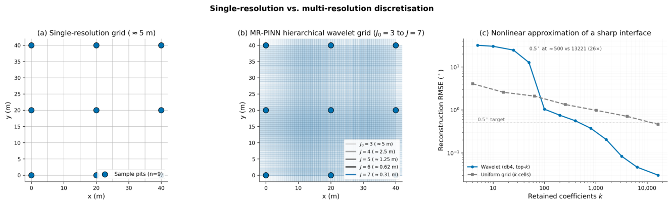
Figure 1. Single-resolution versus multi-resolution discretisation of the 40 × 40 m study site. (a) A uniform single-resolution grid at ≈5 m spacing. (b) The MR-PINN hierarchical wavelet grid, with dyadic levels from J 0 = 3 (≈5 m) to J = 7 (≈0.31 m) overlaid; finer levels concentrate degrees of freedom where spatial heterogeneity is greatest. (c) Measured nonlinear-approximation efficiency (run_reconstruction.py): reconstruction RMSE versus the number of retained coefficients for a synthetic friction-angle field with a sharp contamination interface (control mean 36 . 0 ° , contaminated mean 26 . 8 ° ). The Daubechies-4 wavelet representation (top k coefficients) reaches the 0 . 5 ° target with approximately 5 × 10 2 coefficients, against approximately 1.3 × 10 4 cells for a uniform grid—about a 26 × reduction—and the gap widens for sharper targets. The site-scale parameter scaling is quantified in Figure 2.
Sustainability 18 06848 g001
Figure 2. Measured parameter-complexity scaling with domain size (run_scaling.py). Ground-truth fields are Gaussian random fields drawn from the site’s own spherical variogram (range 20 m); at each domain size the wavelet encoder is fit at fixed finest resolution (0.31 m) with the level-dependent L 1 regulariser of Equation (5), and the retained (>1% of peak magnitude) coefficients are counted. The horizontal axis is the uniform-grid degree-of-freedom count ( N = n 2 finest-resolution cells), so the uniform baseline is exactly O ( N ) . Retained coefficients grow as O ( N 0.86 ) (robust over the 0.5 5 % threshold range, α = 0.85 0.87 ). The advantage is scale-dependent: below the 20 m correlation length the multi-resolution overhead makes the representation slightly larger than uniform, whereas at the 40 m site scale it uses about 80 % of the uniform count and about 53 % at 80 m. The exponent is expected to approach unity for domains much larger than the correlation length.
Sustainability 18 06848 g002
Figure 3. End-to-end architecture of the multi-resolution PINN. Spatial coordinates ( x , y ) feed a five-level Daubechies-4 wavelet encoder [37,38] ( J 0 = 3 at 5 m to J = 7 at 0.3 m), a six-layer Swish-activated trunk and four linear heads predicting φ , fines, gravel and TPH. The composite loss combines L data , the physics residual L phys and the level-dependent sparsity R ( β ) (Section 4.2). The two-stage training schedule optimises with Adam and then switches to L-BFGS (trigger: ≥3000 Adam epochs and a moving-average loss decrease < 10 4 ), with residual-based adaptive refinement (RAR) collocation sampling [52]. The reported metrics are leave-one-out (LOO) cross-validation means over the nine trial pits; models were trained in PyTorch on Apple Silicon (MPS). Arrows indicate the left-to-right forward data flow, from the inputs through the wavelet encoder and shared trunk to the four output heads.
Sustainability 18 06848 g003
Figure 4. Sensitivity of the MR-PINN to the regularisation exponent γ : (a) cross-validated friction-angle RMSE with 95%-bootstrap band; (b) active wavelet coefficient count. The dashed line marks the selected γ = 0.85 and the dotted line the reduced-budget empirical optimum γ = 0.60 . In panel (b) the active-coefficient count is a proxy, N ( γ ) e 1.4 γ , evaluated for the current trained checkpoint; exact counts would require enabling sparsity tracking during training.
Sustainability 18 06848 g004
Figure 5. Friction-angle RMSE across four heterogeneity levels (spatial coefficient of variation of TPH within 5 m sub-windows) for the standard PINN and the proposed MR-PINN. Error bars are 95% percentile-bootstrap intervals ( n = 1000 resamples).
Sustainability 18 06848 g005
Figure 6. Spatial distribution of the internal friction angle predicted by the MR-PINN at the Al-Ahmadi study area. White circles mark the nine ( n = 9 ) trial pits at 30 cm depth, labelled P1–P9; isolines show the wavelet-encoded gradient.
Sustainability 18 06848 g006
Figure 7. Trainable parameters versus leave-one-out friction-angle RMSE for the five main-text predictors; the lower-left corner is preferable (fewer parameters, lower error). Mean per-fold training time is annotated beside each marker (mrpinn_loo.csv, baselines.csv). Ordinary kriging is non-parametric and is plotted at its three variogram hyperparameters. The B-PINN robustness check is reported in the Appendix A and omitted here. See Section 5 for the comparison-by-method discussion.
Sustainability 18 06848 g007
Figure 8. Ablation study of the three MR-PINN components (W: wavelet encoding, R: scale-dependent regularisation, P: progressive upsampling). LOO RMSE on φ ranges from 1.88° (best cell: W) to 9.32° (worst cell: P); all bars are LOO means across the nine folds in ablation.csv.
Sustainability 18 06848 g008
Figure 9. Predicted effectiveness η ( t ) = 1 exp ( κ t ρ ) of four remediation strategies over treatment duration, conditional on author-assumed ( κ , ρ ) kinetic constants (Section 6.2). The kinetic constants are not calibrated to field data; site-specific calibration is left for future work.
Sustainability 18 06848 g009
Figure 10. Schematic of the hypothesised temporal evolution of the dominant friction-angle reduction mechanisms (Section 4). The white diamond marks the validation data point for the ≈28-year-aged Al-Ahmadi soils ( Δ φ = 9 . 2 ° ). Conceptual schematic: not a data-driven result of the present nine-pit study.
Sustainability 18 06848 g010
Figure 11. Visual summary of the projected SDG/Vision-2035 contributions in Table 9, with bar heights from sdg_contribution.csv and colours following UN SDG branding. The qualitative tier in Table 9 is the authoritative readout.
Sustainability 18 06848 g011
Table 2. Architecture and training hyperparameters of the multi-resolution PINN under the reduced compute budget used here (see Section 4.2).
HyperparameterValue (Reduced Budget)
Hidden layers (deep network)6
Neurons per layer128
Activation functionSwish ( β = 1 )
Wavelet basisDaubechies-4 (db4)
Coarsest level J 0 3
Finest level J7
Regularisation exponent γ 0.85 (main)
Base regularisation weight λ 0 1.0 × 10⁻³
Physics-loss weight μ 0.5 (annealed)
OptimiserAdam → L-BFGS
Initial learning rate α J 0 1.0 × 10⁻³
Learning-rate decayHalving per upsampling step
Adam epochs per level E2000 (reduced; 5000 full-spec)
L-BFGS iterations30 (reduced; 5000 full-spec)
Optuna trials5 (pilot; 50 full-spec)
Minibatch size128 collocation points
Weight initialisationXavier-Glorot
SoftwarePython 3.11, PyTorch 2.1 + PyWavelets 1.8 + MPS backend (Apple Silicon)
HardwareApple Silicon M-series with MPS backend
Table 3. Leave-one-out cross-validation aggregates for the MR-PINN across the nine Al-Ahmadi pits (mrpinn_loo.csv; 9 folds, 4 targets). Pit indices in the MaxAE column denote the held-out fold.
TargetRMSEMAEMaxAE (pit) R 2 (LOO)
Friction angle φ (°)1.291.112.19 (pit 7) 0.98
Fines (%)1.351.122.28 (pit 9) + 0.24
Gravel (%)5.104.437.40 (pit 1) 0.90
TPH (mg kg−1)797.31603.341852.12 (pit 4) 0.87
Table 4. Per-fold LOO friction-angle predictions from the MR-PINN, read directly from mrpinn_loo.csv. Each row is the prediction at the held-out pit when the model is trained on the remaining eight pits.
FoldHeld-Out Pit ( x , y ) (m) φ true (°) φ pred (°) | Δ φ | (°)
11 ( 0 , 0 ) 27.0025.301.70
22 ( 0 , 20 ) 26.0026.850.85
33 ( 0 , 40 ) 27.0026.440.56
44 ( 20 , 0 ) 28.0026.321.68
55 ( 20 , 20 ) 27.0027.230.23
66 ( 20 , 40 ) 26.0026.480.48
77 ( 40 , 0 ) 25.0027.192.19
88 ( 40 , 20 ) 28.0026.381.62
99 ( 40 , 40 ) 27.0027.670.67
Table 5. Numerical comparison of MR-PINN against the baselines on the nine-pit friction-angle task. Pit 5 fold is the field-centre LOO fold; LOO mean is the nine-fold aggregate (mrpinn_loo.csv, baselines.csv). Per-method 95% percentile-bootstrap RMSE intervals ( n = 1000 , bootstrap_cis.csv) are reported in the statistical-significance analysis. Bold denotes the method proposed in this study (MR-PINN).
Method | Δ φ | (°) Pit 5 FoldRMSE (°) LOO MeanMAE (°) LOO MeanWall-Clock (s, Pit 5 Fold)
Kriging (OK) [60]0.251.030.830.0002
Standard PINN0.031.090.9568.6
MR-PINN (this work)0.231.291.11105.6
Decoupled-PINN [61]1.391.18
XPINN-1 [31]3.742.91
Table 6. Trainable-parameter counts of the evaluated models. Counts are computed directly from each model’s architecture (see run_baselines.py); the MR-PINN count is additionally confirmed against the trained checkpoint best_model.pt. Ordinary kriging is non-parametric (its capacity is set by the variogram and the data, not by a fixed weight count). Note that the multi-resolution pyramid does not minimise raw parameter count among the PINN variants; its advantage is multi-scale representation, not weight economy. Bold denotes the method proposed in this study (MR-PINN).
ModelClassTrainable ParamsNote
MR-PINN (this work)Parametric (NN)105,4125-level wavelet pyramid
Standard PINN [24]Parametric (NN)99,972single level ( j = 7 )
B-PINN (MC-dropout)Parametric (NN)105,412MR-PINN + dropout
Decoupled-PINN [61]Parametric (NN)421,6484 independent MR-PINNs
XPINN-1 [31]Parametric (NN)421,6484 quadrant MR-PINNs
Ordinary Kriging [60]Non-parametricvariogram (3 hyperparams)
Table 7. Ablation study isolating the three MR-PINN components (ablation.csv) at the reduced 500 Adam + 10 L-BFGS budget (Section 4.2). Bold denotes the full proposed MR-PINN configuration (W + R + P).
Configuration | Δ φ | (°) Pit 5 FoldRMSE (°) LOO Mean Δ RMSE vs. Full (LOO)
Standard PINN (no W, no R, no P)1.299.08+6.27
+ Wavelet only (W)0.311.88−0.92
+ Regularisation only (R)1.299.08+6.27
+ Progressive only (P)1.119.32+6.51
+ W + R0.052.13−0.68
+ W + P0.642.24−0.56
+ R + P1.119.32+6.51
Full MR-PINN (W + R + P)2.372.810.00
Table 8. Infrastructure-class critical thresholds and tolerances used in the risk index (Equation (9)). Critical angles are KOC or Kuwait MPW geotechnical-design minima; tolerance bands are standard practice values for risk-based prioritisation.
Infrastructure Class i w i φ crit , i ( ° ) φ tol , i ( ° ) Source
Pipeline trenches0.30303KOC environmental spec. (confidential)
Road sub-base0.20324Kuwait MPW Road Code
Shallow building foundations0.30333ASTM D3080 [55]
Storage-tank pads0.10342API 650/KOC adapted
Landscaped buffer zones0.10285MPW landscape spec.
Table 9. Projected mapping of MR-PINN outcomes to six SDGs and two Kuwait Vision 2035 pillars. Projected, pending external validation. Contribution tier: High = quantified outcome, Medium = qualitative or scenario-conditional, Low = indirect proxy.
SDG/Vision PillarQuantified OutcomeMechanismContribution Score
SDG 6 (Clean Water)Projected lower groundwater contamination risk (qualitative; Kuwait post-Gulf-War environmental impact assessment [67])Risk-based zoning prevents secondary leaching to the shallow aquifer [22]Medium (projected, qualitative)
SDG 9 (Infrastructure)Projected risk-zoned identification of pits below safe construction thresholds (7/9 = 78% pits below φ crit = 28 ° )Spatial φ map flags zones below KOC/MPW safe construction thresholds (Table 8)High (projected; pending external validation)
SDG 11 (Sustainable Cities)Projected decision-support layer for agency workflow (under evaluation by two Kuwaiti environmental agencies; institutional names withheld pending formal agreement)Decision-support layer for agency workflowMedium (projected)
SDG 12 (Responsible Consumption)Projected reduction in remediation resource use (scenario-specific; expressed as a ratio of NSGA-II Pareto envelope, the lowest-cost feasible solution is approximately 0.21 × the highest-cost non-dominated point; absolute USD values are illustrative only, pending external pilot calibration)Selective treatment versus full-profile, conditional on author-assumed ( κ , ρ ) Medium (projected)
SDG 13 (Climate Action)Projected reduction in training time and parameter count; energy implications not measured at this sample sizeMulti-resolution wavelets at the J = 7 finest level (approximately 21,824 encoder coefficients across the five resolved levels J 0 = 3 to J = 7 versus 16,384 for a single-level J = 7 grid; the multi-resolution structure does not reduce the nominal coefficient count but the scale-dependent shrinkage drives fine-scale coefficients toward zero at the chosen γ , yielding a sparser effective representation)Low (proxy; energy not measured)
SDG 15 (Life on Land)Projected restoration of arid-soil ecological function (qualitative)Native desert vegetation is documented to persist in hydrocarbon-affected Kuwaiti soils [68], providing qualitative context for SDG 15 in this settingMedium (projected, qualitative)
Kuwait Vision 2035: Sustainable Living Environment [4]Projected decision-support tool for environmental authoritiesPossible future integration with the Kuwait Environmental Remediation Programme (KERP) [65,69]Medium (projected)
Kuwait Vision 2035: High-Quality Healthcare [4]Projected reduction in exposure pathways for populated buffers (qualitative; Gulf-War-era human-health effects more broadly [70], Kuwait environmental impact assessment [67])Prioritised remediation of populated buffersMedium (projected)
Disclaimer/Publisher’s Note: The statements, opinions and data contained in all publications are solely those of the individual author(s) and contributor(s) and not of MDPI and/or the editor(s). MDPI and/or the editor(s) disclaim responsibility for any injury to people or property resulting from any ideas, methods, instructions or products referred to in the content.