Input Modality Ablation for Sustainable Landslide Hazard Management Using U-Net: Fused DEM–Optical vs. Spectral vs. Terrain Representations in a Small-Sample Pilot Study

Abstract

Rapid and accurate landslide mapping is essential for disaster risk reduction and sustainable land management in landslide-prone mountainous regions. This study presents a U-Net semantic segmentation framework for pixel-wise landslide classification in the Laonung Creek Watershed of southern Taiwan using 96 annotated tiles derived from a very high-resolution DEM and SPOT-6 multispectral imagery. An input modality ablation experiment compares four configurations: a fused DEM–optical composite matching the visual input used by the annotators (annotation-coherent input), SPOT-6 natural color imagery, a DEM-derived terrain stack, and a six-channel multi-source stack combining all SPOT-6 bands with slope and curvature. All configurations use an identical EfficientNet-B0 U-Net architecture under a spatially blocked train/validation/test design with a fixed held-out test set of 29 tiles. The multi-source stack achieves the highest test Average Precision (AP) of 0.556 (95% CI: 0.463–0.643), whereas the annotation-coherent fused composite achieves AP = 0.511 (95% CI: 0.404–0.601); overlapping confidence intervals indicate that neither modality is definitively superior at this test-set size. The terrain-only configuration (AP = 0.152) confirms that optical information is essential for reliable delineation. A key methodological finding is that differential encoder–decoder learning rates caused rapid decoder overfitting; matched rates of ${10}^{-5}$ substantially stabilized training and are recommended as a conservative default for small-sample segmentation with pretrained encoders. At matched pixel positions, the best DL model achieves AP comparable to a companion Random Forest (DL: 0.847, RF: 0.824), while producing spatially coherent probability maps that support scalable landslide inventory compilation for sustainable hazard management.

1. Introduction

Landslides are among the most destructive natural hazards in mountainous terrain, causing substantial loss of life and infrastructure damage each year [1,2,3,4]. In Taiwan, where steep topography, intense typhoon rainfall, and seismic activity combine to produce exceptionally high landslide activity, rapid and accurate landslide mapping is critical for disaster response, risk assessment, and long-term monitoring [5,6,7,8,9,10]. The Laonung (Laonong) Creek Watershed in southern Taiwan is particularly susceptible, with recurring large-scale landslides triggered by typhoon events that expose extensive areas of bare rock and colluvium on steep slopes in the southern Central Mountain Range [11,12,13,14,15]. Accurate and timely landslide inventory mapping is therefore a prerequisite for sustainable land use planning, infrastructure resilience, and evidence-based disaster risk governance in landslide-prone watersheds such as the Laonung Creek Watershed.

Conventional landslide mapping is commonly based on visual interpretation of aerial or satellite imagery by trained experts. Although this approach can produce reliable results, it is often labor-intensive, time-consuming, and difficult to scale to large areas or frequent acquisition cycles [16]. Automated remote-sensing-based landslide mapping has remained an important research topic for several decades, progressing from pixel-level spectral classifiers [17] through object-based image analysis [18,19] to contemporary machine learning and deep learning approaches [20,21,22]. Despite this progress, several challenges remain unresolved, including severe class imbalance between landslide and non-landslide pixels, ambiguity between landslide surfaces and spectrally similar bare terrain, difficulty in delineating geomorphic unit boundaries (rather than merely identifying spectral patches), and the practical constraint of limited annotated training data in most study areas [23].

Machine learning approaches to landslide mapping have demonstrated strong performance when combined with carefully engineered feature sets derived from multispectral imagery and digital elevation models [24,25,26]. Random Forest classifiers, in particular, have been widely applied because they provide interpretable feature-importance measures and often perform robustly under class imbalance [27,28]. However, pixel-wise classifiers treat each pixel independently, thereby ignoring the spatial context and shape information that are central to geomorphic landslide delineation. As a result, the resulting prediction maps can exhibit spatial noise and may fail to capture the coherent boundaries of landslide geomorphic units [29].

Deep learning, and convolutional neural network (CNN)-based semantic segmentation in particular, offers a well-justified framework for incorporating spatial context into landslide mapping [30]. The U-Net architecture [31], initially proposed for biomedical image segmentation, has since been widely adopted for geospatial semantic segmentation. Its encoder–decoder design and skip connections help retain fine-scale spatial information while exploiting multi-scale contextual features. U-Net-based architectures have been increasingly used for landslide mapping from optical imagery [20,32], synthetic aperture radar [33], and fused multi-source inputs [22,34,35,36], often yielding prediction maps that are more spatially coherent than those produced by pixel-wise classifiers. More recent work has continued to refine encoder–decoder segmentation for landslide mapping, including multiscale attention architectures that sharpen landslide boundary delineation [37] and systematic studies of attention mechanisms and loss-function design in U-Net landslide segmentation with paired optical and DEM inputs [38].

Recent advances in small-sample deep learning for remote sensing semantic segmentation—including semi-supervised learning [39] and self-supervised pretraining [40]—offer promising strategies for improving model generalization under data scarcity. However, their application to landslide mapping remains limited, and the conditions under which pretrained encoder fine-tuning remains stable with small annotated datasets are not well characterized. The present study addresses this gap through a controlled empirical investigation of training dynamics under matched and differential encoder–decoder learning-rate settings.

A continuing challenge in the use of deep learning for landslide mapping is the scarcity of large annotated datasets. Most published DL landslide-mapping studies either use synthetic datasets, aggregate data from multiple events and geographic regions, or evaluate on small test sets without spatially explicit validation [29,41,42]. The risk of spatial leakage—in which training and test pixels are drawn from spatially proximate locations, producing optimistic performance estimates—is widely acknowledged but inconsistently addressed [43,44]. Furthermore, few studies explicitly investigate the contribution of individual input modalities through controlled ablation, making it difficult to isolate the value of terrain-derived features relative to optical imagery [45]. These observations point to three specific gaps that the present study addresses: (i) the absence of rigorously controlled input modality ablation experiments comparing fused DEM–optical composites, spectral-only, terrain-only, and multi-source stacked inputs in landslide semantic segmentation; (ii) the lack of characterization of training stability under small-sample constraints with pretrained encoders, particularly regarding encoder–decoder learning rate configuration; and (iii) the inconsistent application of spatially blocked evaluation designs with explicit uncertainty quantification in DL landslide mapping studies.

This study addresses these challenges through a controlled pilot experiment in the Laonung Creek Watershed, using a carefully annotated dataset of 128 tiles, a spatially blocked train/validation/test design, and a systematic input modality ablation. It is the second of two companion papers based on the same annotated dataset: the companion study [46] (under review) presents an interpretable pixel-wise machine learning approach using Random Forest and gradient boosting classifiers with 13 hand-engineered spectral and terrain features, evaluated under the same spatial blocking scheme. The present study complements that work by replacing hand-engineered features with learned convolutional representations, replacing pixel-wise classification with tile-level semantic segmentation, and explicitly investigating the contribution of four input modality configurations through ablation.

The main goals pursued in this work are outlined below: (1) to conduct a controlled input modality ablation experiment comparing four physically motivated input configurations for U-Net landslide segmentation, including a fused DEM–optical composite designed to match the annotators’ visual input, a spectral-only baseline, a terrain-only baseline, and a multi-source stack, under a rigorous spatially blocked evaluation framework; (2) to introduce and evaluate the annotation coherence principle as a design criterion for input modality selection in expert-annotated remote sensing datasets; (3) to identify and characterize a training instability associated with differential encoder–decoder learning rates in small-dataset settings and to propose a practical resolution within this pilot-study context; and (4) to compare DL segmentation performance against the pixel-wise machine learning results of the companion study [46] on a spatially matched test set, with bootstrap uncertainty quantification.

The remainder of the manuscript is organized in the following manner. Section 2 introduces the study area, dataset, spatially blocked train/validation/test design, input modality configurations, patch extraction procedure, model architecture, training procedure, and evaluation metrics. Section 3 presents the training dynamics, ablation results, test-set evaluation, per-tile analysis, and comparison with the companion study. Section 4 interprets the results in the context of the modality ablation, annotation coherence, small-dataset regularization, and operational applicability. Section 5 synthesizes the principal findings and identifies potential directions for future research.

2. Data and Methods

This section outlines the research setting, input data, and overall framework applied for the analysis. First, the study area and dataset are introduced (Section 2.1). Next, the spatially blocked train/validation/test design used to define the training, validation, and test splits is presented (Section 2.2). The input modalities derived from the DEM and SPOT imagery are then described (Section 2.3), followed by the patch extraction procedure used to generate the model inputs (Section 2.4). The model architecture is subsequently introduced, together with the training procedure (Section 2.5 and Section 2.6). Finally, the inference process and the evaluation metrics used to quantify model performance are presented (Section 2.7).

2.1. Study Area and Dataset

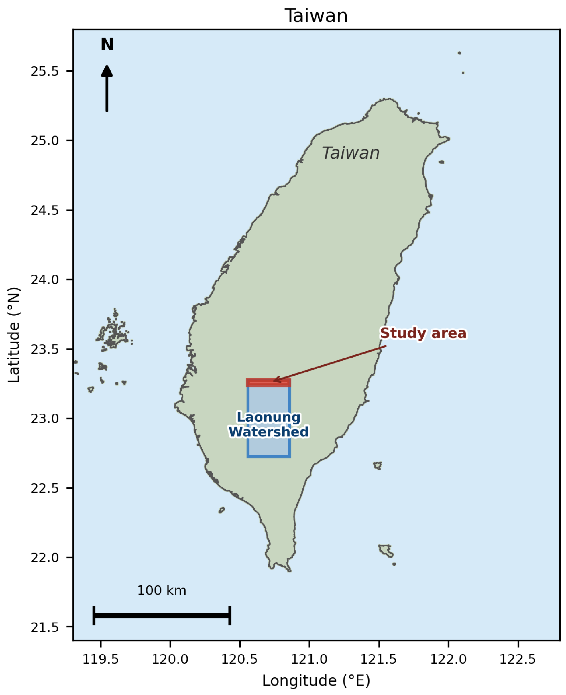
This study focuses on the Laonung (Laonong) Creek Watershed in southern Taiwan (Figure 1), a steep, tectonically active catchment in the southern Central Mountain Range that is highly susceptible to rainfall-triggered landslides. The same dataset described in the companion study [46] is used here without modification; a full description of the data acquisition and annotation procedures is provided therein. For completeness, the key dataset properties most relevant to the present deep learning experiment are summarized below.

The primary elevation data consist of a very high-resolution digital elevation model (DEM), whose resolution is not disclosed for proprietary reasons. The optical imagery consists of SPOT-6 multispectral tiles with four bands (Blue, Green, Red, and Near-Infrared; hereafter B1–B4) acquired at 6 m resolution and resampled to match the DEM. Raw SPOT-6 digital numbers are stored as 12-bit unsigned integers (range 0–4095).

The study domain is partitioned into 2048 tiles of 953 × 947 pixels, arranged in a 64 × 32 grid. Of these, 128 tiles covering rows 1–4 and all 32 columns were manually annotated for landslides by experts, and 96 of them contain landslides. Annotation was performed on a fused composite image, in which a per-band contrast-enhanced SPOT-6 RGB overlay (2nd–98th percentile stretch to 8-bit) was blended at 70% opacity onto a DEM-derived hillshade. Annotators delineated landslide geomorphic units by following optical evidence first and DEM-derived morphology second, with assistance from the Segment Anything Model (SAM 3) [47]. All 96 landslide-positive annotated tiles are used in the current pilot study, and no clean negative tiles within the annotated region are included. The mean landslide areal fraction per tile is 1.7% (range 0.08–9.8%), indicating severe class imbalance at the pixel level. Landslide masks are stored as binary PNG images (0 = background, 255 = landslide).

2.2. Spatially Blocked Train/Validation/Test Split

Spatial autocorrelation is a well-known source of optimistic bias in geospatial model evaluation when training and test samples are drawn from spatially proximate locations [48,49,50,51]. To mitigate this issue, we adopt the same column-quartile spatial blocking strategy used in the companion study [46], partitioning the 96 annotated tiles into four spatially contiguous folds by column range (Figure 2):

• Fold 1: columns 1–8 (23 tiles);
• Fold 2: columns 9–16 (24 tiles);
• Fold 3: columns 17–24 (20 tiles);
• Fold 4: columns 25–32 (29 tiles).

For deep learning, we use a fixed three-way split rather than rotating cross-validation. At this dataset scale, rotating cross-validation would leave fewer than 25 tiles for training in each iteration, which would likely be insufficient for stable U-Net optimization. Folds 1 and 2 (47 tiles) form the training set; Fold 3 (20 tiles) serves as the validation set and is used exclusively for early stopping and model selection; and Fold 4 (29 tiles) serves as the held-out test set and is used only once for final evaluation after all training decisions have been finalized. No tile contributed pixels to more than one split, and tile-level separation was enforced throughout patch extraction, training, and evaluation. The fold assignments used here are identical to those in the companion study [46], ensuring that the test set is spatially matched across both papers and that the comparative analyses in Section 3 and Section 4 are not confounded by evaluation population mismatch.

2.3. Input Modalities

A key element of the present research is the ablation experiment comparing four input modality configurations for the U-Net segmentation model. These four configurations are designed to isolate the contributions of optical imagery, terrain morphology, and their combination to landslide mapping performance (

Table 1. Input modality configurations used in the ablation study. All configurations use an identical U-Net architecture and training procedure; only the input channels differ.

Input	Description	Channels	Source
A	Fused composite (annotation input)	3	Hillshade + SPOT RGB blend
B	SPOT-6 natural color	3	SPOT B3, B2, B1
C	DEM stack	3	Hillshade, slope, curvature
D	Multi-source stack	6	SPOT B1–B4, slope, curvature

).

Input A uses the fused composite image viewed by the annotators during mask delineation. This choice is motivated by annotation coherence: the model is trained on the same visual representation that guided expert landslide delineation, integrating both spectral information and terrain texture into a single three-channel image. In this methodologically informative pilot study, we treat Input A as the primary experiment and the other inputs as ablation comparisons.

Input B uses only SPOT-6 natural color imagery (bands B3, B2, B1 in RGB order), providing a purely spectral baseline without any terrain context. Comparing Input B with Input A isolates the contribution of the embedded hillshade component in the fused composite.

Input C uses a three-channel DEM-derived stack comprising hillshade, slope (in degrees), and profile curvature. Slope angle and profile curvature are physically meaningful predictors of landslide susceptibility because they directly govern the gravitational stress components and hydrological concentration patterns that control slope instability [52]. Steep slopes increase the driving shear force relative to the resisting shear strength of soil, while concave profile curvature promotes pore water pressure accumulation through the convergence of subsurface flow. These morphometric properties are therefore not merely empirical predictors but reflect the mechanical and hydrological processes underlying landslide initiation in the study area. This configuration provides a terrain-only baseline and tests whether morphological features alone are sufficient for landslide delineation in the absence of spectral information, consistent with the annotation protocol in which optical evidence took precedence over DEM-derived features.

Input D combines all four SPOT-6 bands with slope and curvature in a six-channel stack. This configuration provides the richest multi-source input and serves as an exploratory upper bound on performance within the constraints of the available data.

Prior to model input, all channels were normalized using statistics computed exclusively from the 47 training tiles (42.4 million pixels after exclusion of nodata values). SPOT-6 bands were divided by 4095 to map raw 12-bit values to $[0,1]$ and were subsequently z-score-normalized on a per-band basis. Slope and curvature were z-score-normalized directly in their physical units (degrees and raw curvature values, respectively). The fused composite and hillshade channels, both derived from 8-bit PNG images, were divided by 255 and used without z-score normalization. Because no z-score transformation was applied to the fused composite or hillshade channels, their descriptive statistics are not included in

Table 2. Per-channel training-set statistics before z-score normalization, computed from the 47 training tiles (42.4 million pixels after exclusion of nodata values). SPOT-6 values are reported in normalized units (raw digital number divided by 4095). Slope is reported in degrees. Curvature is reported in raw units as output by the terrain analysis software. These statistics were applied identically to validation and test patches.

Modality	Channel	Mean	Std
SPOT-6	B1 (Blue)	0.0724	0.0085
SPOT-6	B2 (Green)	0.0667	0.0146
SPOT-6	B3 (Red)	0.0413	0.0155
SPOT-6	B4 (NIR)	0.1879	0.0858
DEM	Slope (°)	31.61	15.56
DEM	Curvature	$-2.68\times {10}^{-5}$	0.3256

, which reports only the variables for which mean and standard deviation were used in normalization. The training-set normalization statistics were then applied identically to validation and test patches to prevent data leakage. The per-band training statistics before z-score normalization are reported in Table 2.

2.4. Patch Extraction

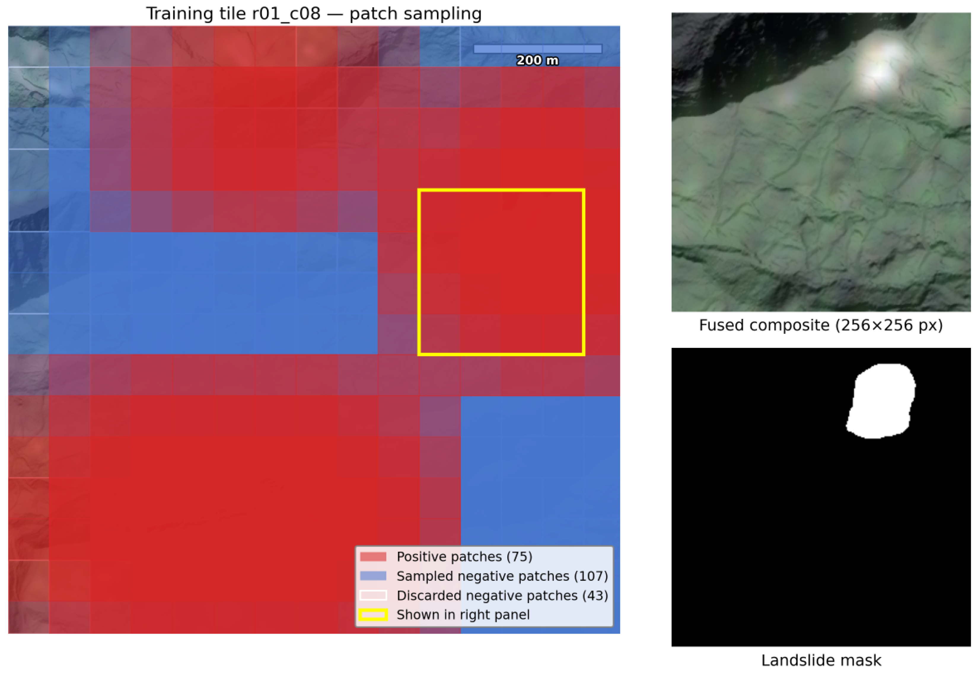
Direct inference on full 953 × 947-pixel tiles is computationally prohibitive for U-Net training because the tile dimensions exceed GPU memory capacity at any practical batch size. We therefore adopt a sliding-window patch extraction strategy (Figure 3).

Patches of 256 × 256 pixels were extracted from all tiles using a stride of 64 pixels, corresponding to a 75% overlap between adjacent patches. Patches extending beyond the tile boundary were zero-padded to 256 × 256 pixels, and the padded areas contained no landslide pixels so that they contributed no gradient during training. A patch was defined as positive if it contained at least one landslide pixel in the corresponding mask.

Patch extraction was applied to all three splits, yielding 10,575 candidate training patches, 1280 validation patches, and 1856 test patches. Because the natural positive patch rate in the training set was 24.6% (2608 positive patches out of 10,575 candidates), we applied stratified subsampling to the training set to increase the frequency with which the model encountered foreground (landslide) pixels during training. All 2608 positive training patches were retained, whereas negative patches were randomly subsampled (seed = 42) so that positive patches constituted 30% of the final training set, yielding 6085 retained negative patches and a total of 8693 training patches. Validation and test patches were not subsampled, thereby preserving the natural class distribution for less biased metric estimation. The resulting patch dataset is summarized in

Table 3. Patch dataset statistics after stratified subsampling of the training set. Positive fraction indicates the proportion of patches containing at least one landslide pixel. The validation and test sets retain the natural class distribution.

Split	Tiles	Patches	Positive	Pos. Fraction
Train (Folds 1 + 2)	47	8693	2608	0.300
Val (Fold 3)	20	1280	220	0.172
Test (Fold 4)	29	1856	496	0.267
Total	96	11,829	3324	0.281

.

During training, patches were loaded from pre-extracted .npy files. Online data augmentation was applied only to the training patches and included random horizontal flipping, vertical flipping, and ${90}^{\circ }$ rotation, each applied with a probability of 0.5. Data augmentation was restricted to the training patches and was not applied to the validation or test sets. These transformations are geophysically reasonable for landslide semantic segmentation because landslide occurrence and morphology do not have a preferred orientation relative to the image acquisition grid.

2.5. Model Architecture

We adopt a U-Net semantic segmentation architecture [31] with an EfficientNet-B0 encoder [53], implemented using the segmentation-models-pytorch library (v0.5.0) [54]. U-Net is built around an encoder component that progressively captures features at multiple spatial scales and an expanding decoder path that recovers spatial resolution through skip connections from the encoder. The EfficientNet-B0 encoder was selected over larger alternatives (e.g., ResNet-50) on the grounds that our training set of 47 tiles would likely be insufficient to support optimization of a substantially larger parameter space without severe overfitting.

The encoder depth was set to 4 (rather than the default of 5) to reduce the receptive field and limit the capacity available for memorizing training patches. This depth setting was chosen based on theoretical considerations regarding receptive field reduction and overfitting mitigation rather than through empirical ablation, and its optimality relative to other depth configurations was not formally evaluated in this pilot study. The corresponding decoder channel configuration is (128, 64, 32, 16), yielding a total of 4,499,405 trainable parameters for three-channel inputs (modalities A, B, and C) and 4,500,269 parameters for the six-channel Input D. The additional 864 parameters in Input D arise from the expanded first convolutional layer, which accepts six input channels instead of three. For all modalities, the encoder was initialized with ImageNet-pretrained weights [55]; for Input D, the first convolutional layer was automatically adapted by segmentation-models-pytorch to accept six channels, with the additional channel weights initialized by averaging the pretrained three-channel weights. A decoder dropout rate of 0.3 was applied to all decoder blocks as a regularization measure. The final layer produces a single-channel output of logits, to which a sigmoid activation is applied externally during loss computation and evaluation.

2.6. Training Procedure

All four modality configurations were trained independently using an identical procedure, differing only in the number of input channels. Model training was conducted for up to 100 epochs, with early stopping used to terminate training when further improvement was not observed. The training hyperparameters are reported in

Table 4. Training hyperparameters. All four modality configurations used identical settings.

Hyperparameter	Value
Architecture	U-Net, EfficientNet-B0 encoder
Encoder depth	4
Decoder channels	(128, 64, 32, 16)
Decoder dropout	0.3
Total parameters (A/B/C)	4,499,405
Total parameters (D)	4,500,269
Encoder initialization	ImageNet pretrained
Loss function	0.5 × Focal + 0.5 × Dice
Focal $\alpha$	0.75
Focal $\gamma$	2
Optimizer	AdamW
Learning rate	$1\times {10}^{-5}$ (encoder and decoder)
Weight decay	$1\times {10}^{-3}$
LR scheduler	ReduceLROnPlateau (factor = 0.5, patience = 7)
Batch size	8
Max epochs	100
Early stopping patience	15
Min AP improvement	0.001
Mixed precision	Yes (torch.cuda.amp)
Random seed	42

. During software implementation, ChatGPT 5 (OpenAI) and Claude Code Opus 4.8 (Anthropic) were used to assist with code development and debugging.

2.6.1. Loss Function

Class imbalance at the pixel level is severe in this dataset: across the 29 test tiles, the positive (landslide) pixel fraction is 2.54%, corresponding to a background-to-foreground ratio of approximately 38:1 at the tile level and a milder ratio at the patch level (2.75:1). To address this issue, we use a combined loss function comprising Focal Loss [56] and Dice Loss [57] in equal proportion:

$$\mathcal{L}=0.5·{\mathcal{L}}_{\mathrm{focal}}+0.5·{\mathcal{L}}_{\mathrm{dice}}$$

(1)

Focal Loss is defined as:

$${\mathcal{L}}_{\mathrm{focal}}=-\alpha {(1-p)}^{\gamma }log\left(p\right)$$

(2)

where p is the predicted sigmoid probability for the positive class, $\alpha =0.75$ is the positive-class weighting factor, and $\gamma =2$ is the focusing parameter that down-weights easily classified background pixels. Dice Loss is defined as:

$${\mathcal{L}}_{\mathrm{dice}}=1-{\displaystyle \frac{2\sum p·y+\epsilon }{\sum p+\sum y+\epsilon }}$$

(3)

where $y\in \{0,1\}$ is the ground-truth mask and $\epsilon =1$ is a smoothing factor used to prevent division by zero. Both loss components were implemented from scratch in PyTorch 2.10.0 (CUDA 12.8 build: 2.10.0+cu128) and operate on raw logits, with the sigmoid applied internally. The combined loss directly encourages foreground overlap (via Dice) while focusing gradient updates on hard and ambiguous pixels (via Focal), which is potentially beneficial for mapping small and low-contrast landslide regions.

The two loss components address class imbalance from complementary perspectives. Focal Loss reduces the contribution of well-classified pixels and places greater emphasis on hard or ambiguous examples, which is particularly useful when easily classified background pixels dominate the training data. In contrast, Dice Loss optimizes the overlap between predicted and ground-truth foreground regions, thereby reducing the influence of foreground–background imbalance compared with purely pixel-wise losses. Nevertheless, each component has limitations when used alone: Focal Loss does not explicitly optimize spatial overlap, whereas Dice Loss may become unstable when the foreground region is very small. Combining the two losses therefore provides a practical way to incorporate both hard-example emphasis and overlap-based optimization. In this study, an equal weighting factor of 0.5 was used as a predefined balanced setting to assign comparable importance to the two objectives, while avoiding the introduction of an additional tunable hyperparameter that would be difficult to justify reliably given the limited training set of 47 tiles.

2.6.2. Optimization

The model was optimized using AdamW [58] with a weight decay of ${10}^{-3}$. Differential learning rates were initially tested (encoder ${10}^{-5}$, decoder ${10}^{-4}$), but they caused the validation AP to peak at epoch 1 across all regularization configurations, suggesting that the decoder was overfitting the training patches before meaningful generalization could develop. 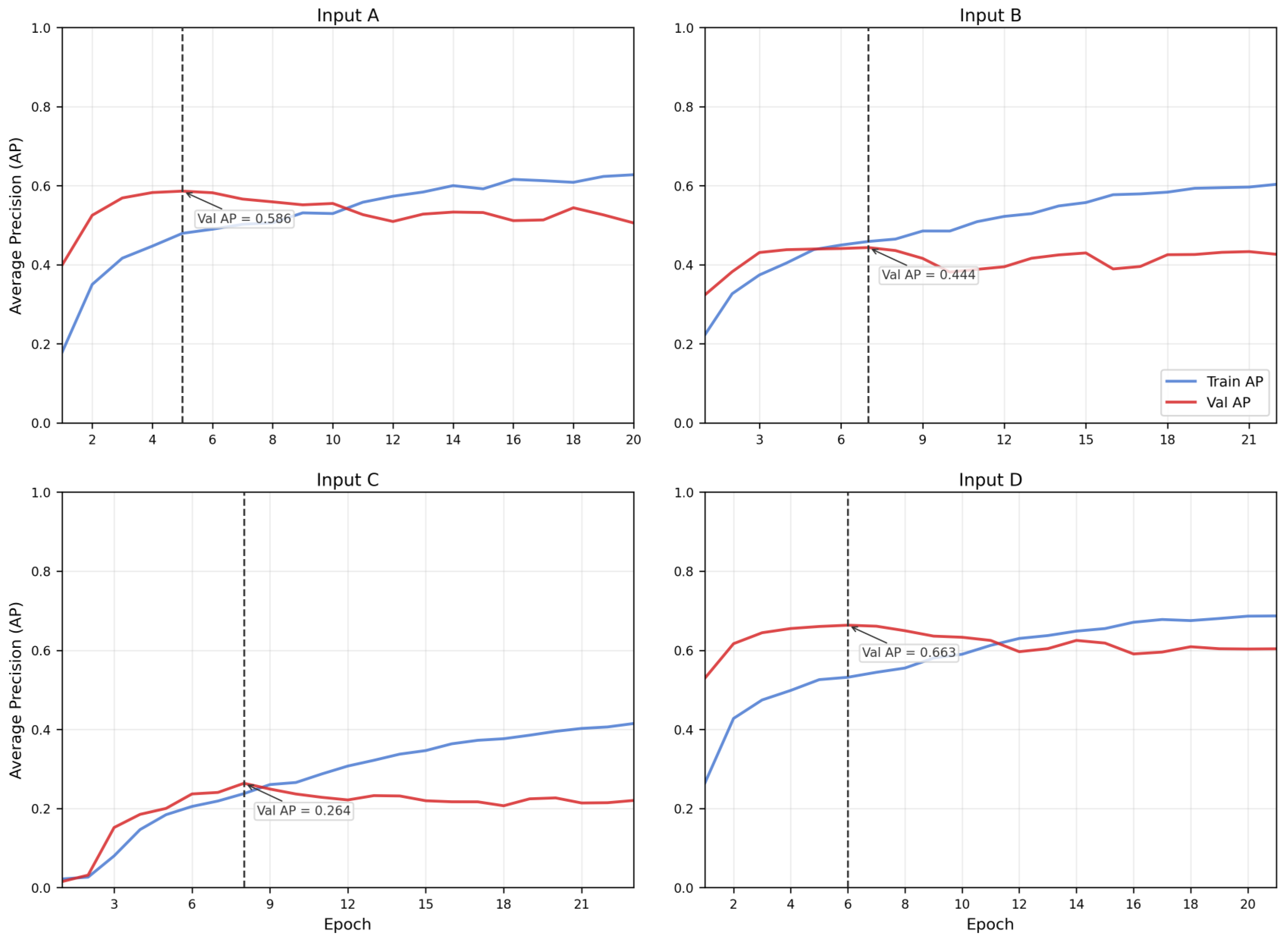Matching the encoder and decoder learning rates at ${10}^{-5}$ mitigated this instability, shifting the best validation epoch from epoch 1 to epochs 5–8 across modalities and nearly doubling the best validation AP for Input A (from 0.306 to 0.586). The matched learning rate of ${10}^{-5}$ was therefore adopted for all modalities in this pilot study. A ReduceLROnPlateau scheduler monitored validation AP with a reduction factor of 0.5, a patience of 7 epochs, and a minimum learning rate of ${10}^{-7}$.

2.6.3. Early Stopping and Model Selection

Early stopping monitored validation AP with a patience of 15 epochs and a minimum improvement threshold of 0.001. For each modality, the checkpoint achieving the highest validation AP was saved and used for all subsequent test-set evaluation. No test-set information was used at any point during training or model selection. Mixed-precision training (torch.cuda.amp) was applied throughout the training process to reduce GPU memory requirements; peak GPU memory usage was 664 MB across all modalities on an NVIDIA GeForce RTX 3050 (8 GB VRAM). Training was conducted with a batch size of 8. All experiments used a fixed random seed of 42 for the random number generators in PyTorch 2.10.0 (CUDA 12.8 build: 2.10.0+cu128), NumPy 2.4.3, and Python 3.11.11, with cudnn.deterministic = True to ensure reproducibility.

2.7. Inference and Evaluation

This subsection describes the inference procedure applied to the held-out test tiles and the metrics used to assess segmentation performance. First, we present the sliding-window inference framework with Gaussian blending used to generate full-tile probability maps and binary predictions. We then describe the evaluation metrics used to assess model performance at both the pixel and tile levels.

2.7.1. Sliding-Window Inference with Gaussian Blending

At inference time, each test tile was processed in full without pre-extraction of patches. A sliding window of 256 × 256 pixels was applied at a stride of 64 pixels, and each patch was passed through the trained model to produce a logit output. To suppress boundary artifacts arising from reduced contextual information near patch edges, predictions from overlapping patches were combined using Gaussian-weighted blending. A 2D Gaussian weight map with a standard deviation of approximately 42.7 pixels (one-sixth of the 256-pixel patch dimension, chosen so that the weight tapers to near zero at the patch edge) was computed once for the 256 × 256 patch size, with unit weight at the patch center and weights tapering smoothly to near zero at the edges. For each pixel in the tile, the blended logit was computed as the weighted mean of all patch logits covering that pixel, with weights given by the Gaussian map at the corresponding within-patch position. A sigmoid function was then applied to the blended logits to obtain a spatially continuous probability map for each tile. Binary predictions were obtained by thresholding at $t=0.5$. Although $t=0.5$ is a customary default for binary segmentation, it remains an arbitrary operating threshold rather than a physically derived cutoff, and different thresholds would shift the precision–recall trade-off. In the present pilot study, we retain $t=0.5$ as a consistent reference threshold across all modalities, while emphasizing probability-based metrics for primary performance comparison. Full-tile probability maps and binary prediction maps were saved as georeferenced GeoTIFF files, inheriting the spatial reference system from the corresponding SPOT-6 tile. Gaussian-weighted blending was adopted over simple averaging or max-pooling because predictions near patch boundaries carry less contextual information than those near the patch center; a formal quantitative comparison of aggregation strategies was not conducted in this pilot study and is identified as a direction for future methodological investigation. On the NVIDIA GeForce RTX 3050 (8 GB VRAM) used in this study, full-tile sliding-window inference at stride 64 required approximately 1.8 min per tile per modality for the 29 test tiles; full-watershed inference across 2048 tiles at a coarser stride required approximately 5–9 s per tile, suggesting that watershed-scale mapping following a triggering event could be completed within a few hours on modest consumer-grade GPU hardware.

2.7.2. Evaluation Metrics

Model performance was assessed primarily using Average Precision (AP), defined as the area under the precision–recall curve. AP was computed from the full precision–recall curve by concatenating predicted probabilities and ground-truth labels across all pixels in all 29 test tiles before computing the curve. Computing AP from the combined full-tile arrays rather than averaging per-patch or per-tile AP estimates is important when positive pixel counts vary substantially across spatial units, as is the case here. Secondary metrics computed at a decision threshold of $t=0.5$ include the F1 score, precision, recall, and intersection over union (IoU). The oracle F1 threshold—the threshold that maximizes F1 on the test-set precision–recall curve—is reported separately as an indicator of the best achievable threshold-dependent performance; it is not used operationally. Per-tile AP was also computed for each of the 29 test tiles to enable spatial analysis of classification performance.

It is important to distinguish this full-tile AP from the matched-pixel AP reported later for comparison with the companion machine learning study. The full-tile AP reported here is computed from all pixels in the held-out test tiles and therefore reflects the natural class prevalence in the study area. By contrast, the matched-pixel AP uses a stratified sample of pixel positions with an elevated positive rate inherited from the companion study design. Because AP is sensitive in practice to class prevalence and sampling composition, these two AP values answer different questions: the full-tile AP is more representative of end-to-end performance on complete tiles, whereas the matched-pixel AP is intended only to support a controlled comparison with the companion pixel-wise classifiers on a common sampled evaluation set.

To quantify uncertainty arising from the small test-set size (29 tiles), 95% bootstrap confidence intervals (CIs) were computed for test AP by resampling the 29 test tiles with replacement (1000 iterations, seed = 42). Tile-level rather than pixel-level resampling was used to preserve the spatial autocorrelation structure of the data. Bootstrap 95% CIs for F1 at $t=0.5$ were computed using the same tile-level resampling procedure, deriving aggregate F1 from summed per-tile true positive, false positive, and false negative pixel counts in each resample rather than averaging per-tile F1 values directly. All metrics were computed in PyTorch on GPU tensors.

2.7.3. Relation to the Companion Study

The companion study [46] evaluated a Random Forest classifier at the pixel level using a stratified sample of pixels drawn from the same 29 test tiles, rather than using all pixels across the full tile extent. Direct comparison of AP between the two studies is therefore complicated by differences in the evaluation populations: the stratified sample used in [46] overrepresents the positive class relative to its natural frequency of 2.54% in the test tiles, thereby inflating AP relative to full-tile evaluation. To enable a like-for-like comparison, we identified the pixel positions sampled in the Random Forest evaluation of [46] within the 29 Fold-4 test tiles and computed DL AP using only those matched positions. This matched-pixel comparison is internally valid for cross-method comparison on a common sampled population, but both values are elevated relative to full-tile AP and should not be interpreted as operationally representative. Accordingly, the primary DL performance metric reported throughout this paper is full-tile AP, whereas the matched-pixel AP is used only to support comparison with the companion study.

3. Results

Although all four models exhibited similarly stable optimization behavior, convergence alone does not indicate whether the learned representations translated into meaningful spatial delineation performance. Because the training set was intentionally limited and the validation criterion was based on Average Precision (AP), it is necessary to examine the extent to which these apparently well-behaved training dynamics were reflected in held-out segmentation performance. The following subsection therefore compares the four input modality configurations in terms of quantitative predictive accuracy and clarifies how differences in input composition affected model performance under the same training and evaluation protocol.

3.1. Training Dynamics

Training curves for all four modality configurations are shown in Figure 4. All models converged within 20 epochs before early stopping was triggered by patience exhaustion. The best validation epochs were epoch 5 (Input A), epoch 7 (Input B), epoch 8 (Input C), and epoch 6 (Input D), indicating stable and consistent training dynamics across the four modality experiments under the chosen seed/configuration. In all cases, training AP continued to increase after the best validation epoch, reflecting a degree of overfitting that is expected given the small training set of 47 tiles. The train-to-validation AP gap was smallest for Input D (best validation AP 0.663, training AP 0.687 at the last epoch), suggesting that the richer multi-source input partially mitigated overfitting by providing a stronger discriminative signal per patch in this pilot-study setting.

An important training instability was identified and resolved during model development. Initial experiments with differential learning rates (encoder ${10}^{-5}$, decoder ${10}^{-4}$) consistently produced the best validation epoch at epoch 1 across all regularization configurations, with validation AP degrading monotonically thereafter despite decreasing training loss. This behavior suggested that the decoder was overfitting the training patches before meaningful generalization could develop, given the strong initial feature representations provided by the pretrained encoder. Reducing both encoder and decoder learning rates to ${10}^{-5}$ mitigated this instability, shifting the best validation epoch to epochs 5–8 and nearly doubling the best validation AP for Input A (from 0.306 to 0.586). This finding has practical relevance for small-sample deep learning with pretrained encoders in this pilot-study context and is discussed further in Section 4.

3.2. Validation-Set Model Selection Results

Validation AP at the best checkpoint followed the ranking D > A > B > C, with values of 0.663, 0.586, 0.444, and 0.264, respectively. This ranking was consistent across the four modality experiments under the chosen seed/configuration and motivated the selection of these checkpoints for final test-set evaluation. The validation results are reported here only as model-selection outcomes and do not constitute the primary performance claim of this study; the test-set results are reported in Section 3.3.

3.3. Test Set Evaluation

Test-set results for all four modality configurations are reported in

Table 5. Test-set performance for all four input modality configurations. AP is computed from the full precision–recall curve over all pixels in all 29 test tiles. Bootstrap 95% confidence intervals (CIs) were computed by tile-level resampling with 1000 iterations. F1, precision, recall, and IoU were computed at a decision threshold of $t=0.5$. Bootstrap 95% CIs for F1 were computed using the same tile-level resampling procedure applied to AP. The oracle threshold is the threshold that maximizes F1 on the test-set precision–recall curve. Val AP is the validation AP at the saved checkpoint and is included for comparison.

Input	Ch.	Test AP	95% CI (AP)	F1	95% CI (F1)	Prec.	Rec.	IoU	Oracle t	Val AP
A	3	0.511	[0.404, 0.601]	0.496	[0.415, 0.570]	0.384	0.698	0.329	0.739	0.586
B	3	0.263	[0.177, 0.366]	0.312	[0.221, 0.424]	0.380	0.265	0.185	0.128	0.444
C	3	0.152	[0.120, 0.198]	0.257	[0.215, 0.296]	0.182	0.437	0.147	0.616	0.264
D	6	0.556	[0.463, 0.643]	0.526	[0.461, 0.587]	0.413	0.723	0.357	0.887	0.663

No-skill baseline AP = 0.025, corresponding to the mean positive pixel fraction in the test set.

and illustrated in Figure 5. The modality ranking on the test set is consistent with the validation ranking: D > A > B > C. Input D achieves the highest test AP of 0.556 (95% CI: 0.463–0.643), followed by Input A at 0.511 (95% CI: 0.404–0.601), Input B at 0.263 (95% CI: 0.177–0.366), and Input C at 0.152 (95% CI: 0.120–0.198). All four modalities exceed the no-skill baseline AP of 0.025, which corresponds to the positive pixel fraction in the test set.

The bootstrap confidence intervals suggest two broad performance tiers. Inputs D and A form the stronger tier, with substantially overlapping CIs, indicating that the observed difference in test AP between these two modalities (0.045) should be interpreted cautiously at this test-set size. Inputs B and C form a clearly weaker tier, with CIs that do not overlap with those of either Input D or Input A. Input C, the terrain-only configuration, is the weakest modality by a substantial margin, with a test AP of 0.152, only modestly above the no-skill baseline.

All models except Input B exhibit a recall-heavy operating profile at the $t=0.5$ threshold: recall ranges from 0.437 (Input C) to 0.723 (Input D), whereas precision ranges from 0.182 (Input C) to 0.413 (Input D). Given the severe class imbalance in the test set, where only 2.54% of pixels are positive, these results indicate that the default threshold favors sensitivity over precision for Inputs A, C, and D. The oracle thresholds further show that the $t=0.5$ operating point is relatively recall-oriented for these modalities: the F1-maximizing thresholds range from 0.739 (Input A) to 0.887 (Input D), with modest F1 gains of approximately 0.033–0.039 over the $t=0.5$ operating point for the better-performing modalities. Input B is an exception to this pattern: at $t=0.5$, it achieves higher precision (0.380) than recall (0.265), indicating that the default threshold suppresses a substantial fraction of true positives. This interpretation is consistent with the low oracle threshold of 0.128 and the complete absence of positive predictions on three of the 29 test tiles (r01_c29, r03_c31, r04_c29), suggesting that the spectral-only input produces probability outputs that are poorly aligned with the default threshold and remain low for many landslide pixels.

A validation-to-test AP drop was observed for all modalities: Input A dropped by 0.075 and Input D by 0.107. This generalization gap likely reflects spatial heterogeneity between the validation fold (columns 17–24) and the test fold (columns 25–32), as well as the inherent optimism associated with model selection on a fixed validation set. The relative ranking of modalities is nevertheless preserved across validation and test, indicating that validation AP served as a useful model-selection criterion in this pilot-study setting even though the absolute values were optimistic.

3.4. Per-Tile Analysis

Per-tile AP for Inputs D and A across the 29 test tiles is shown in Figure 6 and Figure 7. Per-tile AP is highly variable for both modalities: for Input D, per-tile AP ranges from 0.011 to 0.855 (mean 0.552, std 0.220), whereas for Input A, it ranges from 0.003 to 0.836 (mean 0.486, std 0.227). This variability indicates that model performance is strongly tile-dependent and that aggregate test AP can mask substantial spatial heterogeneity in mapping quality.

The relationship between per-tile AP and tile landslide fraction is shown in Figure 6. Pearson correlation coefficients are positive for both modalities (Input D: $r=0.278$, $p=0.144$; Input A: $r=0.350$, $p=0.062$), but neither reaches statistical significance at $\alpha =0.05$ with $n=29$ tiles. The positive direction is consistent with the companion study [46], which found a significant negative correlation between false negative rate and landslide fraction at the pixel level ($r=-0.31$, $p=0.002$), implying that tiles with larger landslide areas tended to be classified more reliably. In the present study, the absence of statistical significance likely reflects the limited test-set size rather than a clear qualitative difference in model behavior; as a result, the pilot test set of 29 tiles provides only limited power to detect a moderate correlation with confidence.

The spatial heatmap in Figure 7 shows that low-AP tiles are not confined to a single geographic subregion within the test fold, suggesting that tile difficulty is more likely to reflect local geomorphic and spectral characteristics than a simple within-fold spatial gradient. Several low-AP tiles also have moderate to high landslide fractions, indicating that landslide classification difficulty depends on factors beyond areal extent, likely including landslide age, vegetation recovery stage, and contrast with the surrounding terrain.

An informative tile-level reversal was observed in the modality ablation: on the representative mid-AP tile r03_c32 (${\mathrm{AP}}_D$ = 0.586, ${\mathrm{AP}}_A$ = 0.789, Figure 8), Input A outperforms Input D despite Input D achieving higher global test AP. This reversal is consistent with the high per-tile AP standard deviation (≈0.22) and indicates that no single modality performs uniformly best across all tiles in this pilot-study setting. It also motivates future investigation of ensemble or adaptive modality-selection approaches.

Figure 9 shows four tiles selected to cover a deliberately diverse set of representative test cases for Input D, rather than only the best predictions. Specifically, tile r02_c28 was selected as a high-AP example near the 85th percentile of the per-tile AP distribution (AP $=0.762$, landslide fraction $=0.0473$), tile r03_c32 was selected as the median-performance example near the 50th percentile (AP $=0.586$, landslide fraction $=0.0485$), and tile r01_c30 was selected as a lower-performing example near the 15th percentile (AP $=0.367$, landslide fraction $=0.0545$). To complement these AP-based cases, tile r04_c32 was additionally selected as a small-landslide example because it contains a very small mapped landslide area (landslide fraction $=0.0028$) while still achieving high per-tile performance (AP $=0.802$). Together, these four tiles illustrate that the probability maps in Figure 9 are intended to represent variation in model behavior across the test set, including strong performance, typical performance, weaker performance, and the special case of successful detection under extremely small landslide extent.

3.5. Comparison with the Companion Study

As described in Section 2.7.3, direct AP comparison between the present study and the companion study [46] is complicated by differences in the evaluation populations. The companion study used stratified pixel sampling, which overrepresents the positive class relative to its natural frequency of 2.54% in the test tiles. On the matched pixel positions from the companion study’s evaluation sample within the 29 Fold-4 test tiles, the Random Forest (RF) model of [46] achieves AP = 0.824, whereas the best DL model (Input D) achieves AP = 0.847. The mean per-tile AP difference (DL − RF) is $+0.019$ (bootstrap 95% CI: $[-0.034,+0.058]$), with the CI crossing zero. At this sample size, the comparison does not provide clear evidence that either model outperforms the other on the matched evaluation set.

These matched-pixel values are elevated relative to full-tile evaluation for both methods and should not be interpreted as operationally representative. Rather, they indicate that the U-Net model achieves pixel-level AP comparable to that of a well-tuned Random Forest on the same sampled spatial test region, without requiring hand-engineered features. Beyond pixel-level accuracy on the matched sample, the DL approach also produces spatially coherent full-tile probability maps (Figure 9) that capture the shape and extent of landslide geomorphic units, whereas pixel-wise classifiers do not directly model such spatial structure.

A direct visual comparison between the best U-Net configuration (Input D) and the companion Random Forest model on representative test tile r01_c25 is shown in Figure 10. Although both models identify a similar central landslide cluster, their spatial prediction behavior differs substantially. The U-Net probability map forms compact and internally coherent high-probability regions that more closely resemble landslide geomorphic units, whereas the Random Forest probability map is more spatially fragmented and exhibits a larger amount of scattered positive response across the surrounding terrain. This difference is further reflected in the binary agreement panel, where disagreement is dominated by RF-only positive pixels outside the central landslide cluster. The tile-level AP values shown in the figure (${\mathrm{AP}}_{\mathrm{U}-\mathrm{Net}}=0.692$, ${\mathrm{AP}}_{\mathrm{RF}}=0.518$) indicate that, for this tile, the U-Net not only provides a more coherent probability field but also achieves stronger tile-level discriminative performance. The example therefore complements the aggregate comparison by illustrating the practical morphological advantage of semantic segmentation over pixel-wise classification in landslide mapping.

4. Discussion

This section interprets the main findings of the study in relation to landslide mapping, model design, and the characteristics of the available dataset. First, the physical implications of the input modality ablation are discussed. Next, we consider annotation coherence as a working hypothesis for modality selection and then examine the implications of overfitting, regularization, and generalization in this small-dataset setting. We then discuss the comparison with the companion pixel-wise machine learning study, followed by the implications of per-tile variability and tile-specific difficulty for interpretation of model performance. Finally, the limitations of the present methodologically informative pilot study and directions for future work are outlined.

4.1. Input Modality Ablation and Physical Interpretation

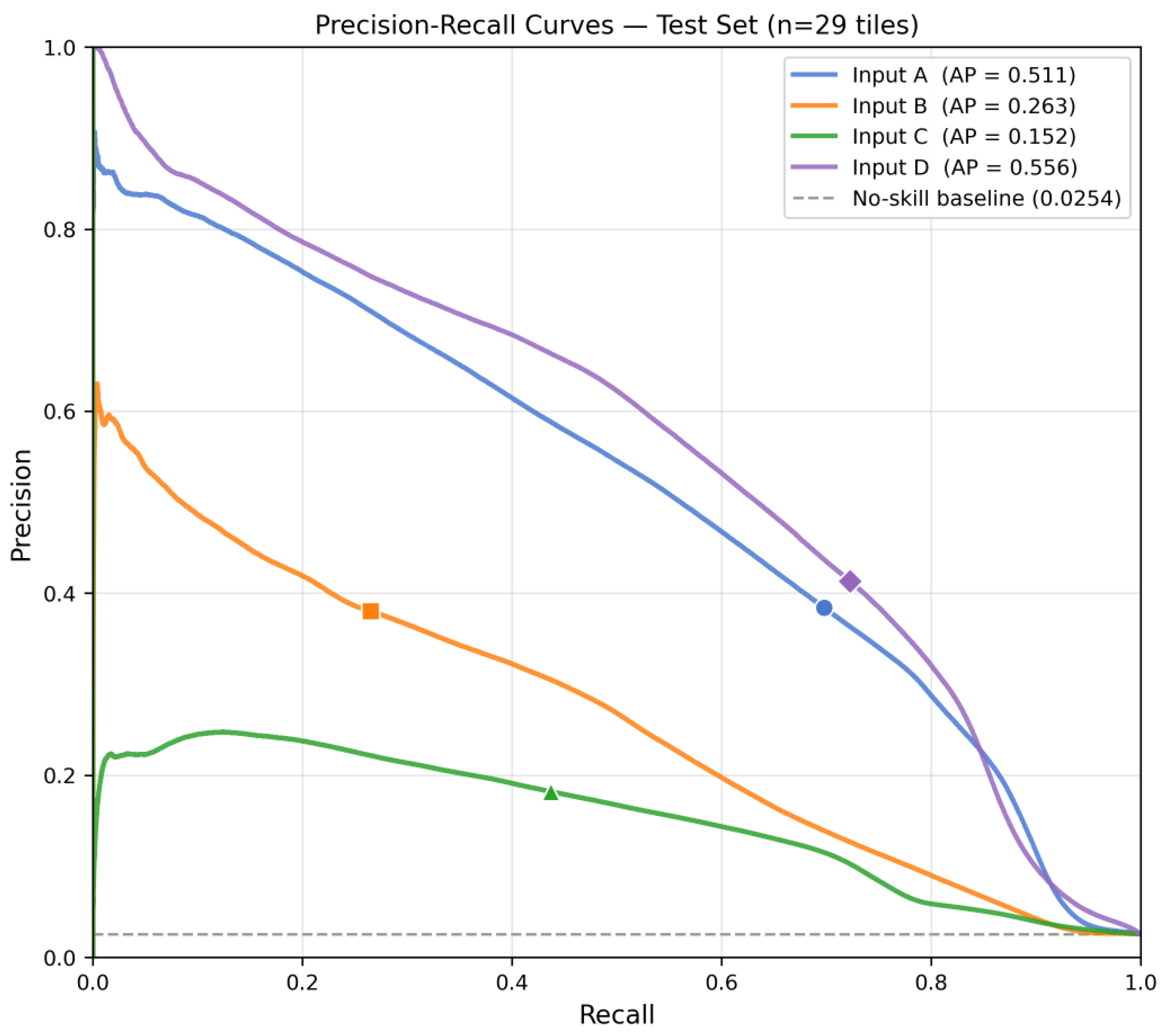
The test AP ranking D > A > B > C is consistent across the validation and test sets and supports a physically coherent interpretation aligned with the known spectral and morphological characteristics of landslides in the study area.

The gap between Input A (fused composite, AP = 0.511) and Input B (SPOT-6 natural color, AP = 0.263) isolates the contribution of the hillshade component embedded in the fused composite. The fused composite blends the hillshade beneath the SPOT-6 RGB overlay at 70% opacity, thereby encoding terrain texture directly into the three input channels. The 0.248 AP difference between A and B therefore provides an empirical indication of the value of this embedded terrain context in the present pilot setting: a U-Net trained on the fused composite can exploit both spectral appearance and terrain surface texture simultaneously, whereas a model trained on natural color imagery alone must rely entirely on spectral discrimination. In the Laonung Creek Watershed, landslide surfaces are often spectrally similar to non-landslide bare soil and exposed bedrock, making pure spectral discrimination inherently ambiguous. The hillshade component appears to provide morphological context that helps reduce this ambiguity, consistent with the annotation protocol in which optical evidence was assessed first, while terrain morphology was used to confirm and refine delineations.

The gap between Input D (multi-source stack, AP = 0.556) and Input A (AP = 0.511) reflects the additional gain obtained by providing terrain features as explicit separate channels rather than as a blended composite. The 0.045 AP difference is modest and falls within the overlapping bootstrap confidence intervals, but it nevertheless suggests a small and consistent benefit from providing slope and curvature as explicit channels rather than relying only on the embedded hillshade representation. This interpretation is physically plausible: slope and curvature encode distinct geometric properties of the terrain surface—gradient magnitude and the rate of change of gradient, respectively—that are not fully captured by a single hillshade channel, which represents illumination from a fixed azimuth and elevation angle. The multi-source stack allows the encoder to exploit these geometric properties independently of the optical signal, which may be particularly helpful for classifying landslides whose spectral contrast with the surrounding terrain is low.

Input C (DEM stack, AP = 0.152) is the weakest modality by a substantial margin, achieving a test AP only modestly above the no-skill baseline of 0.025. In the present pilot-study setting, this result indicates that terrain morphology alone is insufficient for reliable landslide delineation in this watershed at very high resolution. Landslides here are not uniquely defined by terrain shape alone: slope angles and curvature values within landslide boundaries overlap substantially with those of non-landslide steep terrain, gullies, and ridge flanks. Optical evidence therefore appears necessary to distinguish the disturbed, unvegetated surface of a landslide from morphologically similar but vegetated or intact terrain features. This finding is consistent with the annotation protocol, which explicitly prioritized SPOT-6 optical evidence over DEM-derived morphology, and it supports the design choice to treat Input A rather than Input C as the primary experiment in this methodologically informative pilot study.

4.2. Annotation Coherence as a Working Hypothesis for Modality Selection

The selection of Input A as the primary experiment reflects a working hypothesis that we term annotation coherence: when a model is trained on labels produced by human annotators working from a specific visual representation, training the model on that same representation may be preferable to training it on alternative representations, even when those alternatives appear richer in information content. The fused composite was the image viewed by annotators when drawing landslide boundaries; it encodes the visual cues—spectral contrast, terrain texture, and shadow patterns—that expert judgment translated into polygon delineations. A model trained on this representation may therefore be better aligned with the annotation process itself, without requiring the model to bridge a representational gap between its input and the annotation signal. This is an empirical hypothesis that requires further investigation across multiple datasets and annotation protocols.

This principle has practical implications beyond the present study. In remote sensing applications where annotation is expensive and labels are produced from a specific processed product rather than directly from raw sensor data, training on that processed product may yield results that are more consistent with the annotations and more reproducible than those obtained by training on raw or differently processed inputs. The 0.045 AP gap between Input D and Input A on the test set, while favoring the richer multi-source input, is not clearly distinguishable at this sample size, and Input A achieves this performance with a three-channel input that is fully compatible with standard ImageNet-pretrained encoders without any architectural modification. In this pilot-study context, these results suggest that Input A represents a defensible and practically attractive choice when simplicity and reproducibility are prioritized.

4.3. Small-Dataset Deep Learning: Overfitting and Regularization

The training experiments revealed a consistent and practically important finding regarding learning-rate configuration for small-dataset semantic segmentation with pretrained encoders. Initial experiments used differential learning rates, with the randomly initialized decoder updated more rapidly than the pretrained encoder. This strategy was motivated by discriminative fine-tuning approaches, in which different layers are assigned different learning rates to preserve pretrained representations while adapting task-specific layers [59]. However, in the present small-dataset segmentation setting, this configuration caused the validation AP to peak at epoch 1 and degrade monotonically thereafter for all modalities and all regularization configurations tested. The decoder, initialized with random weights and updated at ten times the encoder learning rate (${10}^{-4}$ versus ${10}^{-5}$), appeared to overfit the 8693 training patches within a single epoch, before the encoder had sufficient opportunity to adapt its pretrained representations to the domain-specific characteristics of the DEM and SPOT-6 imagery. Matching both learning rates at ${10}^{-5}$ mitigated this instability, shifting the best validation epoch to epochs 5–8 across all modalities and nearly doubling the best validation AP for Input A.

This finding suggests that differential learning-rate strategies motivated by transfer learning may not transfer directly to small-dataset semantic segmentation when the randomly initialized decoder has sufficient capacity to overfit rapidly. With 47 training tiles and 8693 patches, the decoder may have sufficient capacity to memorize the training distribution rapidly at ${10}^{-4}$, thereby limiting generalization. At ${10}^{-5}$, the slower decoder update rate may encourage the decoder to converge toward solutions that remain more compatible with the encoder’s pretrained feature hierarchy, which may act as an implicit regularizer. In this pilot-study setting, these results suggest that future small-dataset segmentation studies with pretrained encoders should treat the encoder–decoder learning-rate ratio as an important hyperparameter rather than as a fixed design choice, and that matched learning rates may be a reasonable conservative starting point when the training set is limited. We note that this finding is specific to the architecture, dataset, and optimizer configuration employed in this pilot study and should be independently validated before being applied to other segmentation frameworks or datasets.

It is also worth noting that transformer-based architectures and hybrid CNN-transformer models, such as Swin-UNet [60], TransUNet [61], and SegFormer [62], have recently demonstrated strong performance in medical and geospatial image segmentation by exploiting long-range spatial dependencies through self-attention mechanisms. In principle, such architectures could capture broader contextual relationships across the tile extent than a purely convolutional encoder. However, transformer-based models generally require substantially larger training datasets than CNN-based models to converge effectively, and their application in small-sample landslide mapping settings remains an open research question. In the present pilot study, the EfficientNet-B0 encoder was selected specifically for its compact parameter footprint and strong ImageNet-pretrained representations, which are better suited to the available training set of 47 tiles than transformer-based alternatives. Evaluating hybrid CNN-transformer architectures under the same spatial cross-validation framework, when a larger annotated dataset becomes available, is identified as a direction for future work.

Additional regularization measures—decoder dropout of 0.3 and weight decay of ${10}^{-3}$—contributed to training stability but were insufficient on their own to prevent overfitting when the decoder learning rate was set to ${10}^{-4}$. The combination of matched learning rates, dropout, and weight decay produced the best and most consistent results across the four modality experiments under the chosen seed/configuration. Some degree of overfitting remained in all final models—training AP continued to increase after the best validation epoch in every case—but it was reduced to a manageable degree, with the train-to-validation AP gap at the best epoch ranging from −0.132 (Input D) to 0.015 (Input B). The persistence of overfitting is an expected consequence of the pilot-study scale and does not invalidate the test-set results, which were obtained from a checkpoint selected on validation AP without any access to test-set information.

4.4. Comparison with Pixel-Wise Machine Learning

On matched pixel positions from the companion study’s stratified evaluation sample within the 29 test tiles, the U-Net model (Input D) achieves AP = 0.847, compared with the Random Forest’s AP = 0.824. The corresponding mean per-tile AP difference (DL–RF) is +0.019, with a bootstrap 95% CI of $[-0.034,+0.058]$, indicating that the difference is not statistically distinguishable from zero at this sample size. This result should be interpreted cautiously: with 29 test tiles and substantial per-tile AP variability (std $\approx 0.22$), the study has limited power to detect differences of this magnitude. The appropriate conclusion is therefore that the U-Net achieves pixel-level classification performance comparable to that of a well-tuned Random Forest with 13 hand-engineered features, without requiring feature engineering.

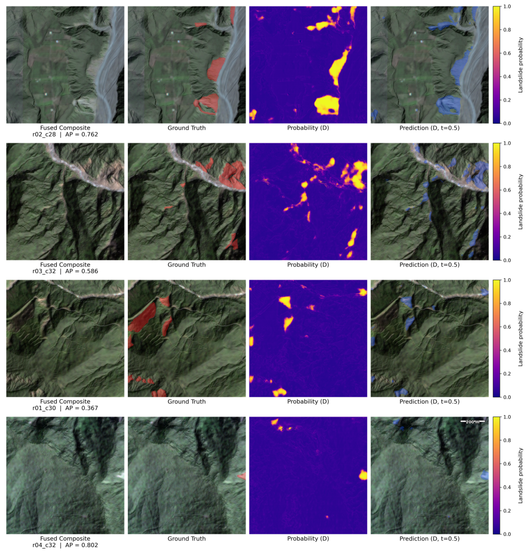
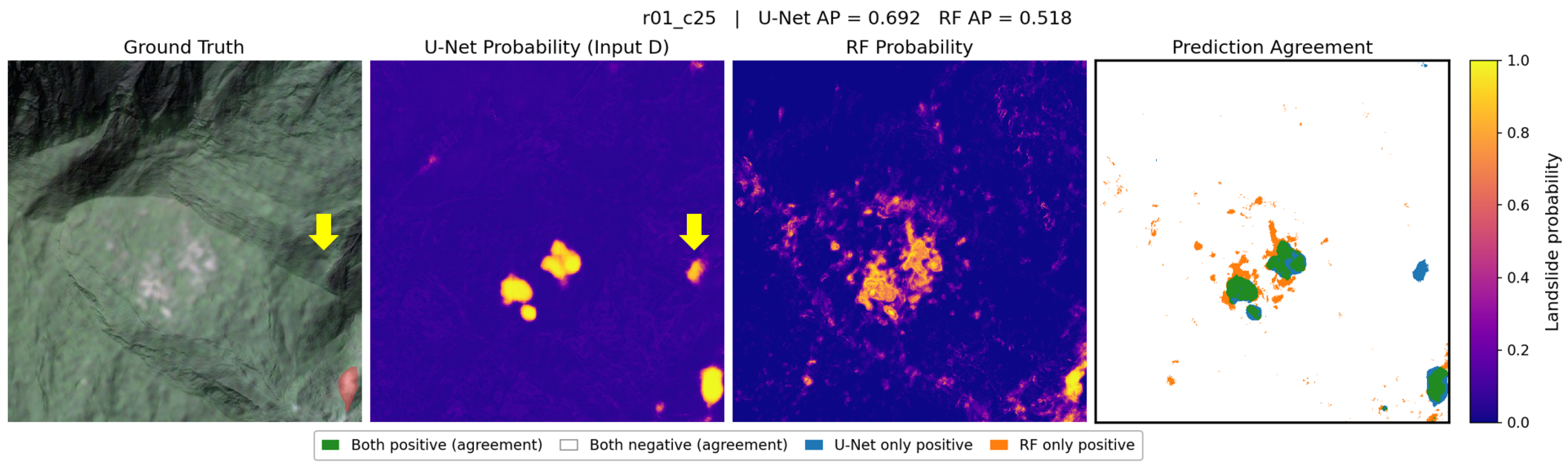
The more substantive distinction between the two approaches lies not in pixel-level AP but in the nature of their predictions. The Random Forest classifies each pixel independently, producing a prediction map in which spatially adjacent pixels are treated as independent observations. The resulting probability maps tend to exhibit salt-and-pepper noise and do not explicitly capture the spatial extent or shape of landslide geomorphic units. The U-Net, operating on 256 × 256-pixel patches with a receptive field spanning tens of meters, learns spatially coherent representations that produce smoother and more geomorphically plausible probability maps (Figure 10). This spatial coherence is not merely aesthetic; it is directly relevant to downstream applications such as landslide inventory compilation, volume estimation, and hazard mapping, all of which require delineation of landslide boundaries rather than only pixel-level binary classification.

A further advantage of the DL approach is its direct applicability to full-tile inference without the need to sample, engineer, and normalize pixel-level features. Once trained, the U-Net processes a full 953 × 947-pixel tile in a single sliding-window pass, producing a georeferenced probability map that can be thresholded, vectorized, and integrated into a GIS workflow without intermediate feature-computation steps. In this pilot-study setting, this operational simplicity, combined with comparable pixel-level accuracy on the matched sampled evaluation set, suggests that the DL approach is a promising direction for future landslide mapping studies in the full Laonung Creek Watershed and similar terrain.

4.5. Per-Tile Variability and Tile Difficulty

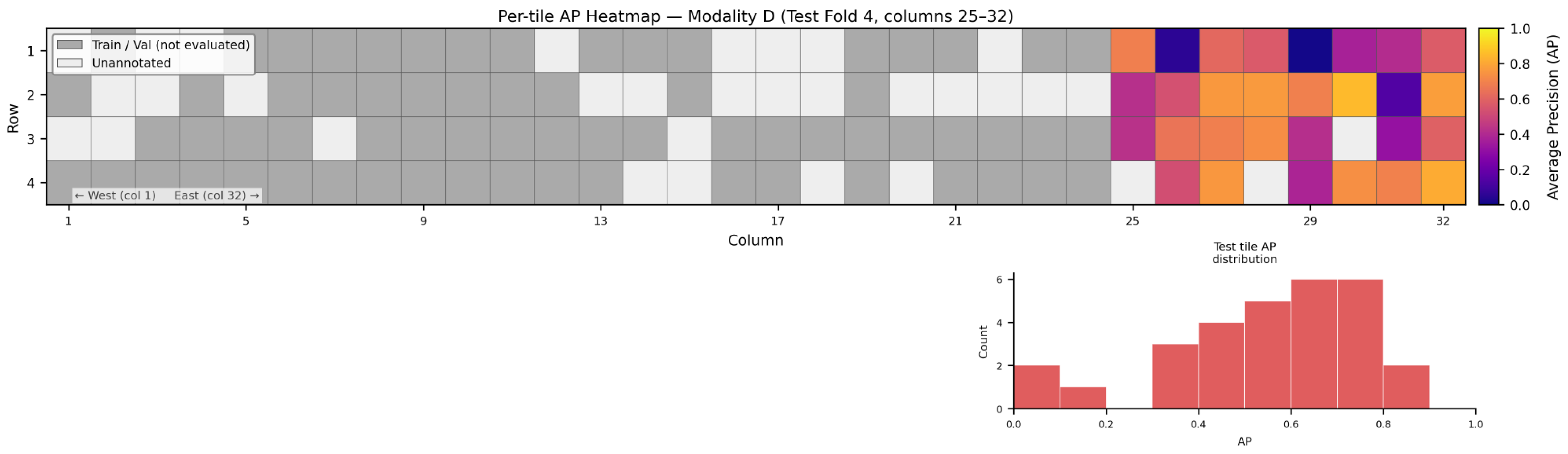
Per-tile AP is highly variable across the 29 test tiles for all modalities (std $\approx 0.22$ for Inputs D and A), indicating that aggregate test AP can mask substantial spatial heterogeneity in classification quality. This variability has two implications. First, aggregate metrics alone are insufficient to characterize model performance for operational interpretation: a model with test AP = 0.556 may achieve AP > 0.85 on some tiles and AP < 0.05 on others, and the spatial distribution of failures is itself geomorphically informative. Second, the wide bootstrap confidence intervals on aggregate test AP (width $\approx 0.18$ for Input D) are a direct consequence of this tile-level variability and reflect genuine uncertainty regarding how the model would perform on a different sample of 29 tiles from the same watershed.

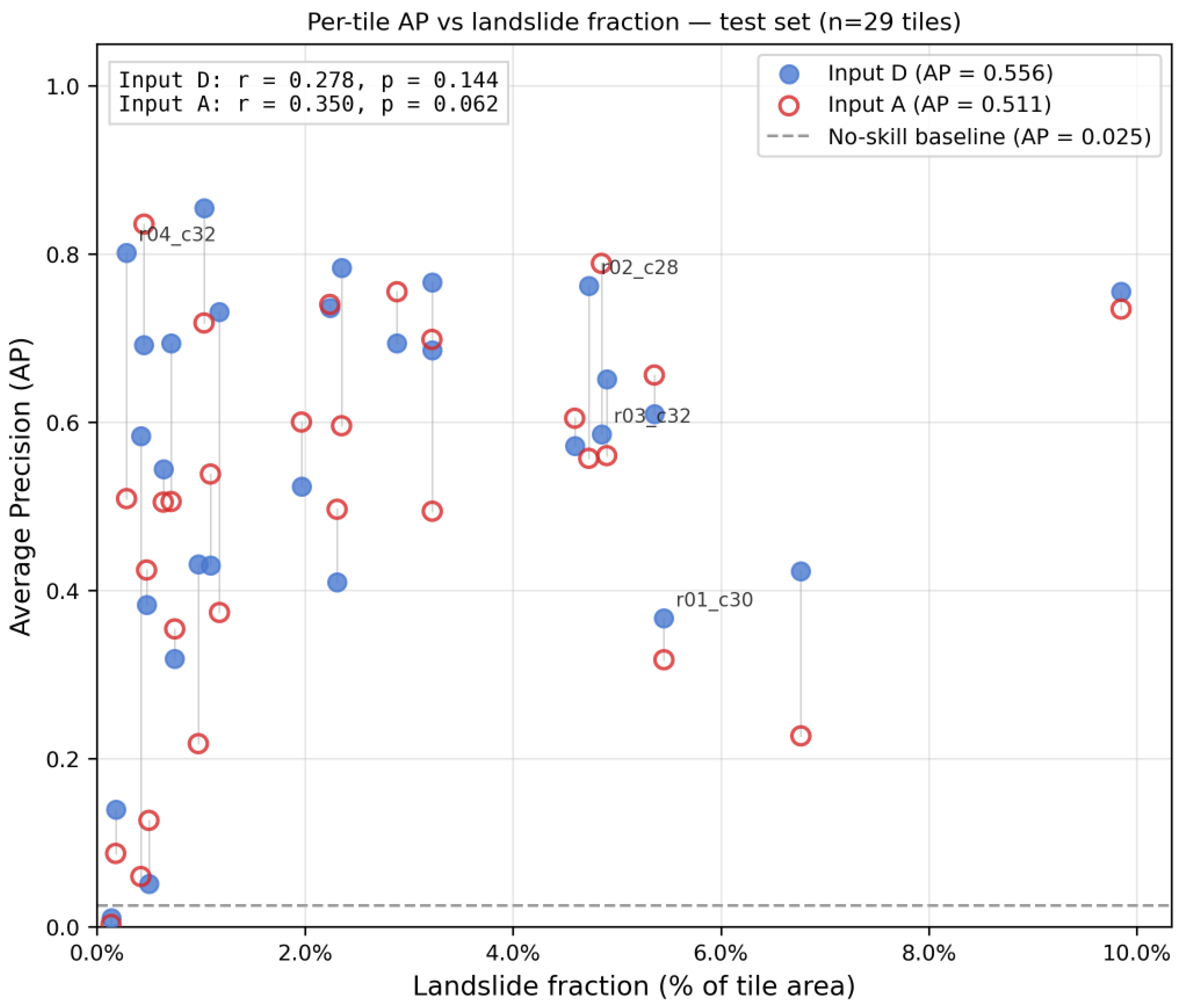
The positive but non-significant correlation between per-tile AP and landslide fraction (Input D: $r=0.278$, $p=0.144$; Input A: $r=0.350$, $p=0.062$) is directionally consistent with the companion study’s finding that false negative rate correlates negatively with landslide fraction [46]. The absence of statistical significance at $n=29$ tiles is not unexpected given the limited statistical power at this sample size and does not contradict the companion study’s finding, which was based on pixel-level analysis across a larger effective sample. The positive direction of the correlation suggests that tiles with larger landslide areas tend to be classified more reliably, likely because larger landslides provide a stronger training signal, are more spectrally and morphologically distinct from their surroundings, and are less sensitive to small boundary-localization errors in the ground-truth mask.

Several low-AP tiles in the spatial heatmap (Figure 7) have moderate to high landslide fractions, indicating that landslide fraction is not the sole determinant of tile difficulty. Other plausible contributing factors include landslide age and vegetation recovery stage—recently triggered landslides with bare, bright surfaces are often more spectrally distinct than older landslides with partial vegetation cover—the degree of spectral contrast between landslide material and the surrounding terrain, the complexity of the landslide boundary relative to the patch size, and possible annotation uncertainty near tile boundaries. Disentangling these factors would require tile-level metadata on landslide age and surface condition that are not available in the present pilot study and is therefore identified as a direction for future work.

The tile-level reversal observed on tile r03_c32—where Input A (AP = 0.789) outperforms Input D (AP = 0.586) despite Input D performing better globally—illustrates that modality superiority is not spatially uniform. This finding motivates future investigation of adaptive or ensemble approaches in which the input modality is selected or weighted according to local terrain and spectral characteristics. A spatially adaptive ensemble that selects between Input A and Input D on the basis of predicted confidence, for example, could in principle outperform either modality alone across the full test set, although this possibility remains to be tested.

4.6. Relevance to Sustainable Disaster Management

Automated landslide mapping contributes to sustainable disaster management by converting remotely sensed imagery and topographic data into spatially explicit information that can support prevention, preparedness, response, and long-term recovery. In mountainous watersheds such as the Laonung Creek Watershed, landslides are recurrent hazards associated with typhoon rainfall, steep terrain, and vulnerable infrastructure corridors. Manually prepared landslide inventories remain essential, but they are labor-intensive and difficult to update frequently over large areas. A scalable deep learning workflow can therefore complement expert interpretation by rapidly identifying candidate landslide areas, producing spatially coherent probability maps, and helping analysts prioritize locations that require detailed inspection. Such information can support disaster management in several ways. First, timely landslide inventories improve post-event situational awareness and help emergency managers identify affected slopes, transportation corridors, and potentially isolated communities. Second, repeated mapping across different image dates can support monitoring of landslide expansion, vegetation recovery, and reactivation, thereby linking short-term disaster response with long-term watershed management. Third, spatially consistent landslide probability maps can inform risk-sensitive land-use planning, slope stabilization priorities, road maintenance, sediment management, and infrastructure resilience planning. Fourth, by reducing the manual burden of inventory compilation, automated mapping can help public agencies allocate limited technical and financial resources more efficiently, especially in regions where recurrent hazards exceed the capacity for exhaustive field investigation. In this context, the present pilot study should not be interpreted as a deployment-ready operational system, because the annotated dataset remains limited and additional validation is still required. Rather, its contribution is methodological: it evaluates how different input representations affect U-Net-based landslide segmentation under a spatially blocked design and identifies practical constraints for small-sample model development. These findings provide a basis for future watershed-scale mapping over the full 2048-tile mosaic, which could support more continuous landslide inventory updating and evidence-based landslide risk management.

4.7. Limitations and Future Work

This study has several constraints that warrant consideration. First, the annotated dataset comprises 96 tiles covering rows 1–4 of the Laonung Creek Watershed, representing a narrow latitudinal strip of the full study area. All 96 tiles are landslide-positive; no clean negative tiles within the annotated region were used, meaning that the model was neither trained nor evaluated on terrain that is entirely free of landslides. The absence of negative tiles may cause the model to overpredict landslides in areas of the watershed where landslides are genuinely absent and precludes evaluation of false positive behavior at the watershed scale. Extending the analysis to include a representative sample of landslide-free tiles is therefore a necessary step before any broader operational use is considered. Future work should also consider pseudo-negative sampling from unannotated tiles outside the annotated region and out-of-distribution detection methods to mitigate the risk of false-positive inflation in landslide-free terrain during operational deployment. Future work should also investigate the probabilistic calibration of the predicted landslide probability maps using metrics such as Expected Calibration Error or Brier Score, which would provide additional insight into the operational utility of the maps beyond the classification metrics reported here.

Second, the fixed three-way spatial split (train: Folds 1 + 2, val: Fold 3, test: Fold 4) does not permit rotating cross-validation, which would provide a more robust estimate of generalization performance across the full annotated domain. At the current dataset scale of 96 tiles, rotating cross-validation would leave fewer than 25 tiles for training in each fold, which would likely be insufficient for stable U-Net optimization. As a consequence, the generalization performance estimated from this fixed partition reflects the specific spatial relationship between the training columns (1–16), validation columns (17–24), and test columns (25–32), and may not be representative of performance under alternative spatial allocations of the same tiles; this sensitivity should be kept in mind when interpreting the test-set results. As the annotation effort expands to cover more rows and columns of the watershed, rotating spatial cross-validation should be adopted in place of the fixed split used here.

Third, the bootstrap confidence intervals on test AP are wide (typical width $\approx 0.18$), reflecting the combined effects of the small test set (29 tiles) and high per-tile AP variability. These intervals quantify genuine uncertainty regarding the generalizability of the results: the predictive performance of the trained models on a different spatial region of the same watershed, or on a different event, remains uncertain. The results reported here should therefore be interpreted as pilot-scale findings that are methodologically informative but do not establish operational readiness. All experiments were conducted under a single fixed random seed (seed = 42), and no multi-seed sensitivity analysis was performed; in small-sample settings, single-run outcomes may be influenced by stochastic initialization effects, and the reported metrics should therefore be interpreted as the result of one specific realization rather than as stable expectations over the initialization distribution. Future work should repeat the full modality-ablation experiment under multiple random initialization seeds, such as 42, 123, and 456, and report the mean ± standard deviation of AP for each input modality to distinguish modality-related performance differences from initialization-induced variability.

Fourth, the decision threshold of $t=0.5$ used for binary prediction maps is retained here as a customary and consistent reference point, but it is not optimized for operational use. The oracle thresholds identified on the test precision–recall curves (0.739 for Input A, 0.887 for Input D) suggest that substantially higher thresholds would improve F1 performance in this dataset, but these thresholds are identified post hoc on the test set and therefore cannot be used operationally without an independent calibration dataset. Future work should include a dedicated threshold-calibration procedure using a held-out calibration tile set.

Future work should prioritize the following directions: expansion of the annotated tile coverage to include multiple rows across the full watershed extent, thereby enabling rotating spatial cross-validation and evaluation on negative tiles; investigation of ensemble and modality-adaptive approaches that exploit the complementary strengths of Inputs A and D at the tile level; incorporation of multi-temporal imagery to capture landslide age and vegetation recovery as additional discriminative features; and application of the trained models to the full 2048-tile watershed mosaic as a first step toward a watershed-scale landslide inventory. Finally, evaluation of the method on independent public landslide segmentation benchmarks, when datasets compatible with the fused DEM–optical input representation become available, would provide external evidence of generalizability beyond the present study area.

5. Conclusions

In this study, landslide mapping is formulated as a semantic segmentation task and addressed using a U-Net model with an EfficientNet-B0 encoder trained on a small annotated dataset of 96 tiles from the Laonung Creek Watershed in southern Taiwan. The primary contributions are an input modality ablation study comparing four configurations spanning fused DEM–optical composites, spectral-only, terrain-only, and multi-source stacked inputs, together with a set of practical findings on training stability and regularization for small-sample deep learning with pretrained encoders.

The main findings are as follows. First, the multi-source six-channel input combining all four SPOT-6 bands with slope and curvature (Input D) achieves the highest test AP of 0.556 (95% CI: 0.463–0.643), followed by the annotation-coherent fused composite input (Input A, AP = 0.511, 95% CI: 0.404–0.601). The confidence intervals of these two top-performing modalities overlap substantially, and neither can be considered definitively superior at this test-set size. The terrain-only input (Input C, AP = 0.152) is the weakest modality, indicating that optical information is important for reliable landslide delineation in this watershed and providing empirical support for the annotation protocol in which SPOT-6 imagery took precedence over DEM-derived morphology.

Second, the fused composite input (Input A) achieves performance comparable to that of the multi-source stack (Input D) while requiring only three input channels that are fully compatible with standard ImageNet-pretrained encoders. This result supports the annotation coherence principle in the context of this pilot study: training on the same visual representation that guided expert annotation can produce models that align effectively with expert judgment without requiring the model to bridge a representational gap between input and label.

Third, a training instability was identified and resolved in which differential learning rates (encoder ${10}^{-5}$, decoder ${10}^{-4}$) caused the decoder to overfit the training patches within a single epoch, thereby limiting generalization. Matching the encoder and decoder learning rates at ${10}^{-5}$ mitigated this instability and nearly doubled the best validation AP for Input A. This finding suggests a practical consideration for small-sample semantic segmentation with pretrained encoders: the encoder–decoder learning-rate ratio should be treated as an important hyperparameter, with matched rates serving as a reasonable conservative starting point when the training set size is limited.

Fourth, on matched pixel positions from the companion study’s evaluation sample, the U-Net (Input D) achieves AP = 0.847, compared with the Random Forest’s AP = 0.824. The corresponding mean per-tile AP difference (DL–RF) is +0.019, which is not statistically distinguishable from zero at $n=29$ tiles (bootstrap 95% CI: $[-0.034,+0.058]$). The DL approach therefore achieves comparable pixel-level classification performance without hand-engineered features while also producing spatially coherent full-tile probability maps that capture the shape and extent of landslide geomorphic units, a capability that pixel-wise classifiers do not directly provide.

Fifth, per-tile AP is highly variable across the 29 test tiles (std $\approx 0.22$ for both top-performing modalities), and the correlation between per-tile AP and landslide fraction is positive in direction but not statistically significant at $n=29$ tiles. This variability underscores the importance of per-tile analysis alongside aggregate metrics and motivates future work to characterize the geomorphic and spectral factors that determine tile-level classification difficulty.

The conclusions drawn from this pilot investigation should be interpreted within the bounds of the annotated Laonung Creek Watershed subset corresponding to rows 1–4 of the tile grid. Three constraints directly limit the reliability of the statistical inferences: the small test set of 29 tiles produces wide bootstrap confidence intervals (typical width ≈ 0.18) that preclude definitive ranking of the top-performing modalities; the fixed three-way spatial split means that generalization estimates reflect one specific spatial allocation of folds rather than an expectation over alternative partitions; and the absence of clean negative tiles means that false-positive behavior in landslide-free terrain remains uncharacterized. Future research should prioritize three directions in order of impact: first, expanding annotation coverage to include negative tiles and multiple watershed rows to enable rotating spatial cross-validation and evaluation under natural class prevalence; second, investigating ensemble and modality-adaptive approaches that exploit the complementary strengths of Inputs A and D at the tile level; and third, applying the trained models to the full 2048-tile watershed mosaic as a first step toward a watershed-scale landslide inventory in support of sustainable hazard management. Together, this study and its companion [46] establish a methodologically rigorous baseline—spanning interpretable pixel-wise machine learning and spatially coherent deep learning—for future landslide mapping studies in the Laonung Creek Watershed.