Research on Traditional Rural Finance, Digital Finance, and Agricultural Economic Resilience: Causal Inference Based on Double Machine Learning

Abstract

Agricultural economic resilience (AER) is not only a key pathway for promoting rural revitalization and ensuring food security, but also an important guarantee for sustainable agricultural development. Based on panel data for 1410 counties in China from 2014 to 2023, this study employs the entropy weight method, a double machine learning model (DML), an instrumental variable model, and a panel threshold model to systematically analyze the impact of traditional rural finance (TRF) on AER and its underlying mechanisms. It also examines the threshold effect of digital finance (DF) in the process through which TRF influences AER, and further explores the roles of DF and TRF in narrowing agricultural development disparities, with the aim of providing scientific evidence for rural revitalization and food security in China and other developing countries, and contributing to the sustainable development of agriculture. The results show that (1) TRF can significantly improve AER, with agricultural technological innovation (ATI) and agricultural socialized services (ASS) playing mediating roles; (2) DF and its dimensions, including coverage breadth, usage depth, and degree of digitalization, exhibit threshold effects in the impact of TRF on AER, and as the levels of DF and its dimensions increase, the positive effect of TRF shows a diminishing marginal trend, indicating a competitive crowding-out effect between the two; (3) the promoting effect of TRF on AER exhibits significant heterogeneity, being stronger in agricultural counties and in the eastern, central, and western regions, following a “Central > Eastern > Western” pattern, while it is not significant in the northeastern region; (4) TRF significantly reduces agricultural development disparities, whereas DF overall significantly exacerbates such disparities, although its different dimensions exhibit clear heterogeneity in their effects, with coverage breadth consistently and significantly widening regional agricultural development gaps.

1. Introduction

Against the backdrop of intensifying global climate change and increasingly stringent resource and environmental constraints, AER serves as an important guarantee for transforming agricultural development from “scale expansion” to “sustainable development”. Rural finance, as the core of the agricultural economy in developing countries, plays an important role in enhancing AER. However, according to Joseph Stiglitz’s theory of imperfect competition, rural financial markets in developing countries are characterized by imperfect information and imperfect competition, and farmers face severe financial exclusion [1,2]. Studies have shown that agriculture in developing countries is predominantly characterized by dispersed smallholder production, which restricts the development of rural financial markets [3]. As one of the developing countries, China has a population of approximately 1.4 billion, accounting for nearly 20% of the world’s total population. However, its per capita arable land area is less than 40% of the global average. Constrained by the widespread distribution of mountainous and hilly terrain and the intergenerational fragmentation of farmland under population pressure [4]. agricultural production in China has long been characterized by fragmented land parcels and small-scale farming operations. According to data from the Third National Agricultural Census released by China’s Ministry of Agriculture and Rural Affairs, more than 98% of agricultural business entities are still smallholders, whose cultivated land accounts for 70% of the total cultivated land, and whose labour force accounts for 90% of the agricultural workforce. According to transaction cost theory, highly fragmented agricultural production increases borrowing costs, thereby significantly reducing the willingness of both lenders and borrowers to participate in credit markets. This not only restricts the growth of rural financial markets but also threatens the sustainability of agricultural economic development. Specifically, the opaque nature of smallholder production, volatile income sources, and a critical lack of acceptable collateral have long posed significant challenges for rural financial institutions in assessing borrowers’ creditworthiness and repayment capacity [5]. This persistent difficulty has restricted the development of China’s rural financial market, furthered the urban-rural loan accessibility gap [6]. impeded agricultural capital formation, and created serious barriers to agricultural technology adoption, productivity gains, and sustainable agricultural economic development [7].

To break this dilemma, China has actively explored a series of solutions by elevating agricultural development to a national strategic level. Through measures such as lowering the entry threshold for rural financial institutions, providing fiscal subsidies for institutions that actively issue agricultural loans, and developing rural DF, China has achieved remarkable results in agricultural development. These efforts have not only strengthened AER but also laid a solid foundation for ensuring food security and promoting rural revitalization. Therefore, taking China as the research object, this paper deeply explores the comprehensive impact of different forms of rural finance on AER, aiming to provide useful experience for the construction of rural financial markets and sustainable agricultural development in China and other developing countries.

Existing studies mainly focus on two aspects: on the one hand, they conduct connotation analysis and quantitative evaluation of AER. The concept of resilience originated in ecology and was later introduced into the analytical framework of economics by C. S. Holling [8]. and further developed into regional economic resilience theory by Ron Martin and others [9,10]. In the field of agricultural economics, AER is defined as the ability of the agricultural system to withstand internal and external shocks, recover from them, and adapt to environmental changes. First, in terms of dimensional division, existing studies generally follow a three-stage analytical paradigm of “resistance-recovery-adaptability.” Specifically, resistance reflects the ability of the agricultural system to maintain normal production and effectively reduce potential losses when facing external risks. This ability is closely related to factors such as basic agricultural production conditions [11]. production scale, and production capacity [12]. Recovery reflects the ability of the agricultural system to adjust its production and management strategies flexibly and to quickly return to its original production level in the face of uncertain shocks [13]. A strong agricultural economic foundation, farmers’ economic strength, government fiscal support, and improved educational levels can provide sufficient economic and human capital to support rapid recovery [14]. Adaptability reflects the ability of the agricultural system to improve productivity through transformation and innovation after experiencing shocks, thereby achieving transformation and upgrading and maintaining sustainable development in a new environment [13]. Second, in terms of measurement methods, existing literature mainly adopts two approaches: one is the composite index method, which constructs a multidimensional indicator system based on entropy weighting or principal component analysis to generate a resilience index; the other is the core variable method, which typically uses agricultural output as a proxy variable. Based on these methods, scholars have conducted systematic evaluations of AER at different spatial scales in China. The results show that China’s AER exhibits an upward trend and a spatial pattern characterized by “higher in the east and lower in the west, higher in plains and lower in mountainous areas.” [11].

On the other hand, some scholars have begun to focus on the empowering effect of financial factors on AER. These studies can be summarized as follows: through the three major functions of resource allocation, risk management, and information production, the financial system can effectively alleviate liquidity constraints and uncertainties faced by agricultural entities when responding to shocks, thereby improving AER. First, regarding TRF, scholars have, based on rural financial development theory, demonstrated that high-quality rural financial development has a positive effect on AER [15]. Its mechanisms can be summarized into three aspects: (i) consumption and investment smoothing, where credit availability helps farmers maintain necessary production inputs after shocks and avoid falling into a “poverty trap”; (ii) risk diversification, where financial tools such as agricultural insurance distribute individual risks across a broader scope through the law of large numbers; (iii) incentives for technology adoption, where long-term and stable financial support reduces the risk premium associated with adopting resilient varieties or adaptive technologies, thereby enhancing adaptability capacity. Second, regarding DF, as an emerging financial form, scholars have begun to examine its empowering effect on AER. Studies show that DF reshapes the risk response logic of agricultural systems through the following channels [16]. (i) reducing information asymmetry, as big data technologies enable credit profiling for smallholders lacking collateral; (ii) reducing transaction costs, as mobile payments significantly lower the cost of accessing financial services; (iii) expanding financial accessibility, as DF breaks geographical constraints and enables remote areas to access financial services.

Although existing studies have made significant progress in TRF, DF, and AER, which provide a solid theoretical foundation for this study, there are still three main limitations. First, from a research perspective, existing studies mostly examine TRF and DF separately and fail to integrate them into a unified framework. In reality, agricultural business entities may both receive offline services from rural financial institutions and use online DF channels. Whether these two financial forms are complementary or substitutive remains unclear. Whether the development of DF alters the effect of TRF on supporting agriculture remains unanswered. Second, in terms of research methodology, most existing studies adopt traditional linear regression models, which make it difficult to identify the net effect in causal inference accurately. This is because AER is a comprehensive indicator influenced by multiple economic and social factors, and traditional models are prone to specification bias when dealing with high-dimensional control variables. Third, regarding data, most studies rely on provincial or municipal-level data. However, there are significant differences in agricultural resource endowments and rural financial development across counties in China. Coarse-grained data are difficult to capture structural characteristics at the county level, and also make it difficult to effectively evaluate the role of different financial forms in narrowing agricultural development disparities.

In view of this, this study, based on panel data from 1410 counties in China from 2014 to 2023, deeply examines the impact and transmission mechanisms of TRF on AER, as well as the threshold effect of DF in this process. Further, it analyzes the role of these two financial forms in narrowing agricultural development disparities. First, based on financial development theory, the theory of creative destruction, and transaction cost theory, this study systematically analyzes the theoretical logic by which TRF and DF affect AER, thereby expanding the research perspective in this field. Second, based on the “pressure-state-response” framework, a comprehensive evaluation index system of AER is constructed, covering risk resistance capacity, recovery and adaptability capacity, and innovation and transformation capacity. Using data from 1410 counties in China, the entropy weight method is employed to measure the development level of AER. Finally, using DML as the core empirical method, this study empirically analyzes the impact of TRF on AER and its transmission mechanisms, and employs a panel threshold model to explore the threshold effect of DF. On this basis, the study further analyzes the role of TRF and DF in narrowing agricultural development disparities.

The remaining structure of this study is as follows: Section 2 presents the theoretical analysis and research hypotheses; Section 3 discusses the research methodology and model construction, and explains variable definitions and data sources; Section 4 reports the baseline regression results, robustness checks, and endogeneity treatment; Section 5 conducts heterogeneity analysis; Section 6 further discusses the role of TRF and DF in narrowing agricultural development disparities; and Section 7 presents the conclusions and policy implications.

2. Theoretical Analysis and Research Hypotheses

2.1. Theoretical Mechanism Between TRF and AER

According to rural financial development theory, TRF can provide credit support to agricultural business entities to alleviate financial constraints, thereby improving agricultural infrastructure and increasing the level of agricultural mechanization, which in turn enhances AER. Specifically, agricultural production usually relies on a relatively high level of agricultural infrastructure and mechanization input. Whether it is the construction and maintenance of farmland irrigation and water conservancy facilities, or the purchase and upgrading of agricultural machinery, all require substantial financial support. TRF, by being rooted in local counties, can shorten the distance between financial institutions and farmers, thereby reducing information asymmetry to some extent and enhancing mutual trust, which, in turn, increases the likelihood of farmers obtaining credit [17].

In addition, according to the theory of optimal financial structure [18]. new agricultural business entities, such as family farms and farmers’ professional cooperatives, often find it difficult to obtain credit from large commercial banks due to the lack of effective collateral and standardized credit records [19]. In this context, TRF can leverage its geographical advantages to obtain “soft information” (such as reputation, social relationships, and community standing) on agricultural business entities to assess their credit risk [6]. thereby promoting the formation of “relationship-based lending” [20]. Continuous credit support helps improve agricultural infrastructure and enhance agricultural mechanization [21].

Based on this, the following hypothesis is proposed:

H1. 

TRF development can enhance AER.

2.2. Mediation Mechanisms of TRF Affecting AER

2.2.1. Agricultural Technological Innovation

Agricultural technological innovation enhances AER by strengthening the agricultural system’s resistance, recovery, and adaptability capacities. Specifically, according to the “creative destruction” theory proposed by Joseph Schumpeter, technological innovation in agriculture optimises the economic structure by eliminating inefficient production methods and promoting the reallocation of factors [22]. First, agricultural technological innovation reduces the impact of natural disasters and market fluctuations on agricultural output by promoting stress-resistant varieties and water-saving irrigation technologies, thereby enhancing the agricultural system’s risk-resistance capacity. Second, agricultural technological innovation improves the efficiency of factor allocation and the speed of information response, enabling agricultural business entities to flexibly adjust production decisions and enhance their adaptability to changes in the external environment. Finally, agricultural technological innovation promotes the continuous evolution of agricultural production methods and industrial structures, facilitating the dynamic reorganization of resources across different production links, and enabling a transition from “recovery-based growth” to “transformational growth,” thereby strengthening the adaptability capacity of the agricultural system after shocks.

In this process, the realisation of agricultural technological innovation depends heavily on sustained financial support. At the same time, TRF creates opportunities for such innovation by alleviating credit constraints and providing risk-sharing mechanisms. On the one hand, improvements in credit availability reduce the financing costs and uncertainties faced by agricultural business entities in adopting technology and investing in R&D, thereby encouraging forward-looking technological investment. On the other hand, long-term financial support based on relationship-based lending helps share the risks in the process of technological innovation, reduces the “trial-and-error cost,” and thus increases the probability of agricultural technological innovation. Therefore, TRF can achieve a multidimensional enhancement of AER by promoting agricultural technological innovation.

Based on this, the following hypothesis is proposed:

H2a. 

TRF development indirectly enhances AER by promoting agricultural technological innovation.

2.2.2. Agricultural Socialized Services

Agricultural socialized services mainly enhance AER by improving the agricultural system’s resistance and recovery capacities. Specifically, based on the division of labor theory and transaction cost theory, as specialization deepens and transaction costs decline, agricultural production has gradually shifted from a self-sufficient model dominated by smallholders to a collaborative production model dominated by socialized services [23,24]. In this process, agricultural socialized services effectively reduce farmers’ risk when facing natural disasters and market fluctuations by providing standardized and large-scale agricultural machinery operations and plant protection services, thereby enhancing the agricultural system’s risk-resistance capacity. At the same time, the service outsourcing mechanism reduces farmers’ decision-making costs in information search, technology selection, and production processes, enabling them to flexibly adjust cropping structures and production arrangements, thereby improving their capacity to recover from external shocks.

In comparison, the impact of agricultural socialized services on the adaptability capacity of the agricultural system is more reflected in the gradual optimization of production organization rather than structural transformation driven by technological breakthroughs, and therefore its effect is relatively lagged. On this basis, the development of agricultural socialized services depends heavily on financial support. TRF guides the allocation of agricultural production resources by alleviating financing constraints on both the supply and demand sides. On the one hand, from the supply side of agricultural socialized services, credit support from TRF helps service organizations invest in equipment and expand scale, thereby improving the stability and coverage of service provision. On the other hand, from the demand side, financial resource allocation reduces constraints on agricultural business entities’ access to socialized services, promotes their integration into a specialized division of labor system, and reduces efficiency losses and risk exposure arising from fragmented operations. Therefore, TRF enhances AER by promoting the development of agricultural socialized services, thereby improving the agricultural system’s resistance capacity and adaptability.

Based on this, the following hypothesis is proposed:

H2b. 

TRF development indirectly enhances AER by promoting agricultural socialized services.

2.3. Theoretical Logic of the Threshold Effect of DF

In the digital era, the rise of DF is reshaping the rural financial ecosystem, making the impact of TRF on AER no longer a simple linear relationship. Treating the DF level as a threshold variable to examine the nonlinear impact of TRF is a necessary supplement and refinement to the mechanism analysis. Specifically, DF exhibits stage-based threshold effects. In the early stage of DF development, due to the need for digital infrastructure support, farmers typically rely on accounts opened in traditional rural financial institutions when using digital financial services [25]. Therefore, DF mainly plays an auxiliary role at this stage, while TRF remains dominant in supporting agriculture. When DF enters a mature stage, the advantages of big data technologies gradually emerge, enabling it to break geographical constraints and reduce information asymmetry and customer acquisition costs [26], thereby generating a competitive crowding-out effect on TRF. As a result, competition from DF suppresses the expansion of traditional rural financial institution outlets. Although such competition may promote the optimization of outlet layouts for rural financial institutions [27]. this optimization is usually constrained by multiple factors such as costs and geographical conditions, and the space and effect of optimization are limited. Therefore, at this stage, DF gradually replaces part of TRF’s service functions, thereby weakening TRF’s positive promotional effect on AER.

Furthermore, different development dimensions of DF also have heterogeneous impacts on the above relationship. First, at a low level of coverage breadth, DF’s accessibility is limited, and TRF remains the main provider of financial services. As coverage breadth increases, DF gradually attracts TRF’s original customers, thereby weakening TRF’s role in supporting agriculture. Second, at a low level of usage depth, the application of DF by agricultural business entities remains at a basic functional level and cannot effectively compete with TRF [28]. as usage depth increases, DF gradually acquires the ability to compete with TRF, thereby crowding out its role. Finally, at a low level of digitalization, DF is not yet well developed in terms of operational efficiency and risk control; as digitalization improves, its service efficiency and risk control capabilities continue to strengthen, thereby forming a competitive crowding-out effect on rural financial institutions.

Based on this, the following hypothesis is proposed:

H3. 

The impact of TRF on AER exhibits nonlinear threshold characteristics depending on the level of DF development.

3. Research Design

3.1. Research Method

3.1.1. DML Model and Logic of Algorithm Selection

This study adopts the DML model to examine the impact of rural financial institutions and DF on AER and its regional heterogeneity. Because traditional linear regression models have substantial limitations in sample requirements and variable selection, and that nonlinear relationships between variables can easily lead to estimation bias, as well as the possibility that a large number of variables may generate multicollinearity and dimensionality issues [29]. DML can effectively compensate for the shortcomings of traditional linear regression models. While flexibly controlling high-dimensional covariates, it can obtain robust estimation and inference of causal effects [30].

Compared to traditional linear regression models, DML is better suited to the research questions of this study. Empirical evidence from Victor Chernozhukov et al. [31]. indicates that when treatment effects are heterogeneous across individuals or control variables change over time, DML can yield more reliable and robust causal estimates than traditional linear regression models. Chen Gang and Chen Yunshan [29]. also argue that DML has unique advantages in capturing heterogeneity in treatment effects and dynamic changes over time, which provides an important methodological foundation for this study. On the one hand, in China, there are significant regional differences in natural resource endowments and economic development foundations, and there are also obvious differences in the development of rural financial institutions and AER across counties, as further confirmed by the heterogeneity analysis later in the study. On the other hand, AER is a complex composite index influenced by multiple socioeconomic factors, and the relationships among variables are often nonlinear. Traditional linear regression models are difficult to capture such high-dimensional features, which may lead to estimation bias.

Therefore, this study follows the DML framework proposed by Chernozhukov et al. [32]. to identify causal effects and constructs the following partially linear model:

$$AE{R}_{it}={\theta }_{0}TR{F}_{it}+g\left(X_{it}\right)+U_{it},E\left(U_{it}\right|TR{F}_{it},X_{it})=0$$

(1)

$$TR{F}_{it}=m\left(X_{it}\right)+V_{it},E\left(V_{it}\right|X_{it})=0$$

(2)

In Equations (1) and (2), i denotes a county, and t denotes a year; Equation (1) is the basic regression equation, and Equation (2) is the auxiliary regression equation; $AE{R}_{it}$ denotes the dependent variable, and $TR{F}_{it}$ denotes the core explanatory variable; ${\theta }_0$ is the coefficient of interest in this study; $X_{it}$ is the set of multivariate control variables for each county; the specific forms of the functions $g\left(X_{it}\right)$ and $m\left(X_{it}\right)$ are unknown and must be estimated using machine learning algorithms to obtain $\widehat{g}\left(X_{it}\right)$ and $\widehat{m}\left(X_{it}\right)$; $U_{it}$ and $V_{it}$ are both error terms, each with a conditional mean of 0.

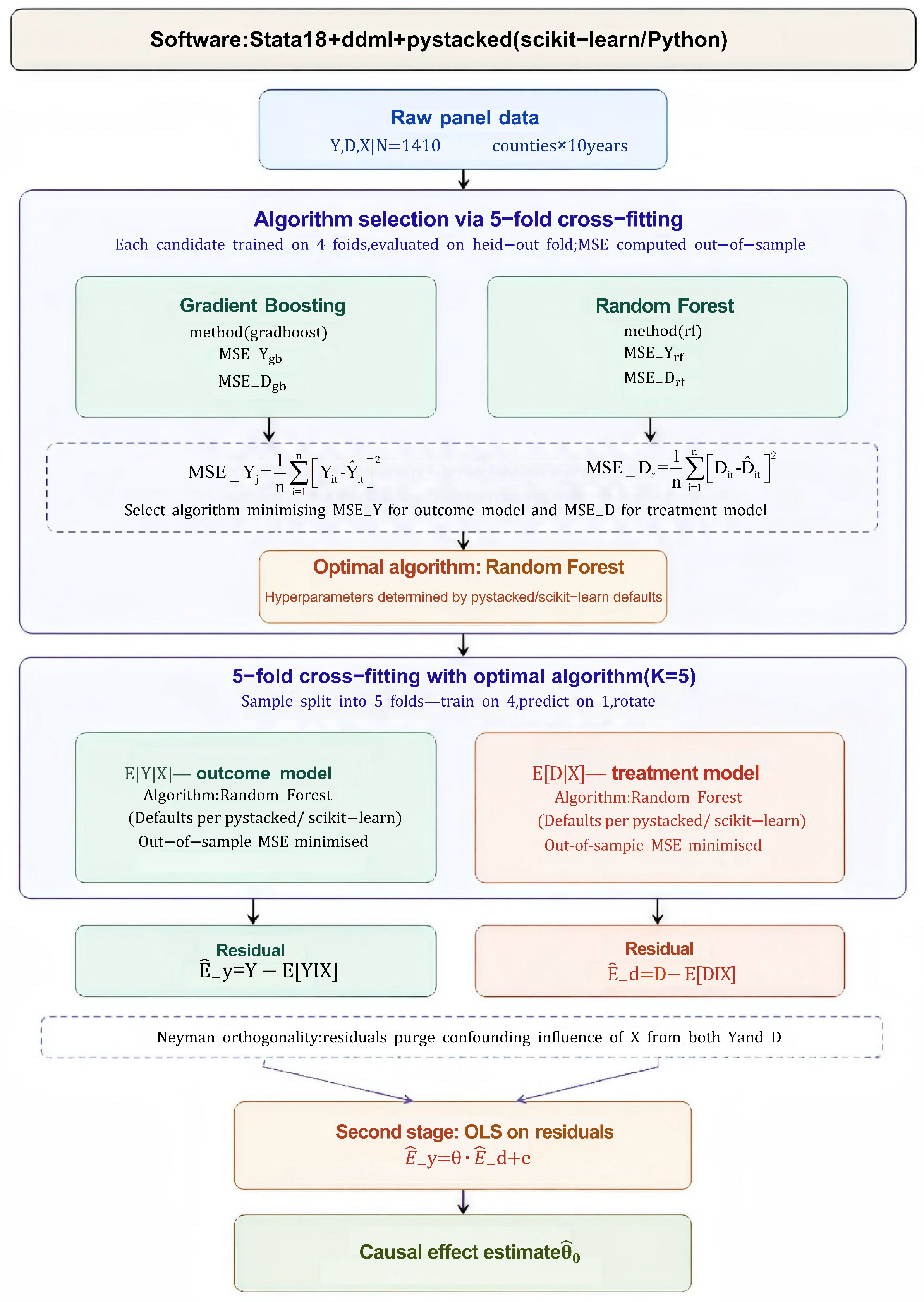
The estimation procedure for the causal effect is as follows. First, the data are partitioned into K mutually exclusive subsamples for cross-fitting. For the k-th subsample, the remaining K − 1 subsamples are used to estimate function $m\left(X_{it}\right)$ in Equation (2) using machine learning algorithms, yielding estimator $\widehat{m}\left(X_{it}\right)$. Subsequently, the estimator $V_{it}$ of the residual term ${\widehat{V}}_{it}=TR{F}_{it}-\widehat{m}\left(X_{it}\right)$ is obtained. Second, following the same procedure, estimator $g\left(X_{it}\right)$ of function $\widehat{g}\left(X_{it}\right)$ in Equation (1) is estimated, yielding $AE{R}_{it}-\widehat{g}\left(X_{it}\right)={\theta }_{0}TR{F}_{it}+U_{it}$. Finally, ${\widehat{V}}_{it}$ is used as an IV for $TR{F}_{it}$ in a linear regression, from which the estimate ${\widehat{\theta }}_0$ of ${\theta }_0$ is obtained. The standard errors, confidence intervals, and statistical inference for ${\theta }_0$ are identical to those in ordinary linear regression:

$${\widehat{\theta }}_0={\left({\displaystyle \frac{1}{n}}\sum _{i\in I,t\in T}{\widehat{V}}_{it}TR{F}_{it}\right)}^{-1}{\displaystyle \frac{1}{n}}\sum _{i\in I,t\in T}{\widehat{V}}_{it}\left(AE{R}_{it}-\widehat{g}\left(X_{it}\right)\right)$$

(3)

It is worth noting that the DML model includes various algorithms, but which is the most optimal? Currently, there is no unified conclusion on this issue. To address this, and different from studies that only adopt a single algorithm, to avoid potential incidental bias caused by using a single model, following Hu et al. [30]. this study uses two commonly applied decision tree-based algorithms, namely random forest and gradient boosting, to calculate the mean squared error (MSE) through cross-fitting. It selects the algorithm with the minimum MSE as the optimal algorithm combination.

In addition, to improve the robustness of the conclusions, this study, based on the above decision tree models, further introduces three major categories of commonly used models: generalized linear models, neural network models, and kernel-based methods. Specifically, for generalized linear models, Lasso regression and elastic net are selected; for neural network models, a standard neural network is used; and for kernel-based methods, the support vector machine (SVM), which has relatively better performance, is selected. The optimal algorithm combination is then re-selected to test the baseline regression results. In this way, the models used in this study cover the four major categories commonly applied in the DML framework, namely generalized linear models, decision tree models, neural network models, and kernel-based methods, to achieve cross-validation among multiple models and improve the reliability of the conclusions of this study. Specifically for this study, the procedure for selecting the optimal algorithm combination is as follows:

First, divide the research data into K mutually exclusive subsamples. For the kth subsample, apply the jth, rth, and sth machine learning algorithms to the remaining $K-1$ subsamples to obtain the estimates ${\widehat{Y}}_{it}$, ${\widehat{D}}_{it}$, and ${\widehat{Z}}_{it}$.

Second, for the jth, rth, and sth machine learning algorithms, we calculate the MSE using cross-validation, as follows:

$$MSE\text{\_}{Y}_j={\displaystyle \frac{1}{n}}{\displaystyle \sum _{i=1}^n}{\left[Y_{it}-{\widehat{Y}}_{it}\right]}^2$$

(4)

$$MSE\text{\_}{D}_r={\displaystyle \frac{1}{n}}{\displaystyle \sum _{i=1}^n}{\left[D_{it}-{\widehat{D}}_{it}\right]}^2$$

(5)

$$MSE\text{\_}{Z}_s={\displaystyle \frac{1}{n}}{\displaystyle \sum _{i=1}^n}{\left[Z_{it}-{\widehat{Z}}_{it}\right]}^2$$

(6)

Next, select the optimal algorithms j, r, and s for Equation (4) through (6), respectively, to form the optimal algorithm combination, as follows:

$$JR=\min \left[MSE\text{\_}{Y}_j+MSE\text{\_}{D}_r\right]$$

(7)

$$JRS=\min \left[MSE\text{\_}{Y}_j+MSE\text{\_}{D}_r+MSE\text{\_}{Z}_s\right]$$

(8)

Finally, based on Equations (7) and (8), the optimal algorithm combination is used to estimate the impact of TRF on AER.

In Equation (4) through (7), K represents the number of subsamples and also serves as the cross-validation split ratio. The variables j, r, and s denote the machine learning algorithms for the base regression equation, the auxiliary regression equation, and the instrumental variable auxiliary regression equation, respectively. i denotes the sample individual, t the year, and n the total number of samples. $Y_{it}$, $D_{it}$, and $Z_{it}$ represent the dependent variable, the core explanatory variable, and the instrumental variable (IV), respectively, ${\widehat{Y}}_{it}$, ${\widehat{D}}_{it}$ and ${\widehat{Z}}_{it}$ represent the predicted values of $Y_{it}$, $D_{it}$ and $Z_{it}$, respectively. Equation (4) is MSE of the base regression equation estimated using algorithm j. Equation (5) is the MSE of the auxiliary regression equation estimated using algorithm r. Equation (6) is the MSE of the IV auxiliary regression equation estimated using algorithm s. In Equation (7), JR is the optimal algorithm combination for the basic and auxiliary regressions, selecting j and r to minimize $MSE\text{\_}{Y}_j+MSE\text{\_}{D}_r$, in Equation (8), JRS is the optimal algorithm combination for the basic, auxiliary, and IV auxiliary regressions, selecting j, r, and s to minimize $MSE\text{\_}{Y}_j+MSE\text{\_}{D}_r+MSE\text{\_}{Z}_s$.

Furthermore, according to Chernozhukov et al. [32]. DML achieves better fit performance when the number of cross-fitting folds (K) is set to 5. Therefore, when estimating the effect of TRF on AER using the DML model, this study primarily reports the results from 5-fold cross-validation. Meanwhile, to visually illustrate the application logic of the above DML approach, a methodological flowchart is presented in Figure 1.

3.1.2. Threshold Effect Model

In addition, to examine the threshold effects of DF and its dimensions—coverage breadth, usage depth, and digitalization level—in the relationship between TRF and AER, this study follows the threshold regression model approach proposed by Hansen [33] and constructs the following threshold panel regression model:

$$AE{R}_{it}={\beta }_0+{\beta }_{1}TR{F}_{it}\times I(q_{it}\le \gamma )+{\beta }_{2}TR{F}_{it}\times I(q_{it}>\gamma )+{\beta }_3{X}_{it}+{\mu }_i+{\delta }_t+{ϵ}_{it}$$

(9)

In Equation (9), $q_{it}$ is the threshold variable, $\gamma$ is the threshold value. ${\beta }_0$ and ${\beta }_1$ are the intercept term and treatment coefficient, respectively. $I(·)$ is an indicator function, equal to 1 if the condition in parentheses holds and 0 otherwise. ${\mu }_i$ and ${\delta }_t$ are the individual fixed effect (time-invariant) and year fixed effect, respectively. ${ϵ}_{it}$ is the random disturbance term. Other variables are as defined in Equations (1) and (2).

Due to space limitations, only the single-threshold case of the threshold panel regression model is presented above. However, multiple thresholds may also exist. Since the multiple-threshold model is similar to the single-threshold model, it will not be elaborated here. However, multiple thresholds were tested and reported in the empirical analysis in the following sections.

3.2. Variable Selection

3.2.1. Dependent Variable

Resilience primarily refers to a system’s ability to withstand and recover from external shocks and disturbances. The concept originated in ecology and was later introduced into the analytical framework of economics by Holling [8]. Subsequently, Martin et al. [9]. developed the theory of regional economic resilience and defined economic resilience as the ability of a region to withstand market shocks, competition, and environmental factors while recovering to its original economic state or achieving structural improvement. Building on the concept of economic resilience, subsequent scholars further defined AER as the ability of an agricultural economic system to withstand, recover from, and adapt to external shocks and disturbances [34].

Given this, it is evident that AER is a multidimensional composite concept, and a single indicator is insufficient to fully capture its core connotation. To address this complexity, and drawing on the “pressure–state–response” theory proposed by Martin et al. [9]. as well as the research findings of multiple scholars [11,13,15,35,36,37,38]. this study constructs a comprehensive evaluation index system for AER (see

Table 1. Comprehensive evaluation index system for AER.

Dimension	Variable Name	Variable Definition	Direction	Weight	Symbol
Resistance	Usable arable land	Usable arable land area	+	0.087	C1
	Primary industry employment	Number of employees in primary industry	+	0.084	C2
	Fiscal self-sufficiency	General public budget expenditure/general public budget revenue	−	0.049	C3
	Agricultural cooperatives	Number of specialized farmer cooperatives	+	0.005	C4
	Scale of agricultural industrialization	Number of active primary industry enterprises	+	0.102	C5
	Grain production capacity	Total grain output	+	0.066	C6
Recovery	Gross output of the primary industry	Gross output of the primary industry	+	0.051	C7
	Fiscal expenditure on agriculture	Expenditure on agriculture, forestry, and water affairs	+	0.038	C8
	Rural income level	Per capita disposable income of rural residents	+	0.029	C9
	Education level	Primary & secondary school enrollment/total county population (year-end)	+	0.021	C10
	Growth rate of primary industry value added	(Value added of the primary industry − base period value)/base period value	+	0.021	C11
Adaptability	Agricultural mechanization level	Total agricultural machinery power	+	0.061	C12
	Informatization level	Broadband subscribers/total number of households at year-end	+	0.032	C13
	Agricultural R&D personnel capacity	Full-Time Equivalent of Research and Experimental Development Personnel in Agriculture	+	0.102	C14
	Intensity of agricultural R&D expenditure	Intramural Expenditure on Research and Experimental Development	+	0.106	C15
	Agricultural entrepreneurship activity	Number of newly established new-type agricultural business entities/administrative region area	+	0.146	C16

Note: “+” indicates a positive indicator; “−” indicates a negative indicator.

). Additionally, to ensure objectivity in measurement, the entropy weight method is employed.

(1) Resistance Capacity: The resistance capacity refers to the ability of the agricultural economic system to maintain normal agricultural production and to effectively mitigate potential losses in the face of external shocks. Its capacity to cope with and absorb risks is often closely associated with factors such as basic agricultural production conditions, production scale, and production capacity. Therefore, commonly used indicators, including cultivated land area, the number of employees in the primary industry, the level of fiscal self-sufficiency, the coverage rate of agricultural cooperatives, the degree of agricultural industrialization, and grain production capacity, are selected as measures of this dimension.

(2) Recovery Capacity: Recovery capacity refers to the ability of the agricultural economic system to flexibly adjust its production and operational strategies and to rapidly return to its original production level in the face of uncertain shocks. A strong agricultural economic foundation, farmers’ economic strength, government fiscal support for agriculture, and improvements in educational attainment can provide sufficient economic and human capital to quickly restore the agricultural system’s production capacity after shocks. Therefore, the total output value of the primary industry, county-level fiscal expenditure on agriculture, rural residents’ income level, educational attainment, and the growth rate of the primary industry’s value added are selected as indicators for measurement.

(3) Adaptive Capacity: Adaptive capacity refers to the ability of the agricultural economic system, after being subjected to uncertain shocks, to improve agricultural productivity through transformation and innovation, achieve structural upgrading of production and operation, and maintain sustainable development in a new environment. Therefore, indicators such as agricultural mechanization productivity, county-level informatization, agricultural science and technology talent support capacity, the intensity of expenditure on agricultural science and technology activities, and the level of agricultural entrepreneurship activity are selected as measurement indicators.

In summary, each of the above indicators is selected based on the core connotations of resistance, recovery, and adaptive capacity in AER. This ensures that the assessment of AER is grounded in a solid theoretical foundation and rooted in the practical needs of sustainable agricultural development, such as food security, cultivating talent in agricultural science and technology, and fostering innovation and entrepreneurship.

3.2.2. Core Explanatory Variable

The core explanatory variable in this study is the level of TRF development. TRF refers to a form of finance that primarily relies on traditional financial institutions, such as rural commercial banks and rural credit cooperatives, and provides credit, savings, settlement, and other financial services to rural residents and agricultural business entities through offline physical outlets and manual approval mechanisms [39,40]. Given that banking institutions have long dominated China’s rural financial system, following Hua and Li [6]. this study uses the number of rural financial institution outlets as a proxy variable. The specific types of institutions include rural commercial banks, rural credit cooperatives, rural cooperative banks, rural mutual aid cooperatives, village and township banks, and loan companies. To mitigate the impact of differences in county size, following Tan and Tian [41]. the number of outlets is standardized by administrative area to construct an indicator of rural financial institution outlet density. It should be noted that this indicator mainly reflects the spatial accessibility of rural financial services.

3.2.3. Mediating Variables

Based on the “creative destruction” and transaction cost theories, this study selects agricultural technological innovation and agricultural socialized services as mediating variables. In terms of agricultural technological innovation, following the study by Sun et al. [36]. the number of agricultural science and technology patent applications is used as the measurement. In terms of agricultural socialized services, considering its important role in promoting the deepening of division of labor, optimizing resource allocation, and reducing transaction costs, and following Yuan et al. [42]. as well as data availability, this study uses the number of newly established agricultural service organizations, and further standardizes it by administrative region area to measure the development level of agricultural socialized services.

3.2.4. Threshold Variables

The threshold variables in this study are the level of DF and its three dimensions: coverage breadth, usage depth, and digitalization level. International studies generally define DF as an important form of financial service provision through emerging channels such as mobile payments, mobile banking, and digital platforms. By integrating modern digital technologies into financial services, DF can effectively expand coverage and improve accessibility [43]. The Peking University Digital Financial Inclusion Index comprehensively reflects the development of DF at the county level and has been widely used in studies on DF in China. Therefore, this study employs this index to measure the level of county-level DF development and further conducts analyses based on its three dimensions: coverage breadth, usage depth, and digitalization level.

3.2.5. Control Variables

To ensure the accuracy of causal identification, this study also controls for other factors that may affect AER, as follows (see

Table 2. Definition and descriptive statistics of main variables.

Variable Name	Variable Definition	Obs	Mean	S.D.
AER	AER composite index	14100	0.1657	0.0782
TRF	Number of RFI branches per km2	14,100	0.0192	0.0216
Agricultural Technological Innovation	Log (Number of agricultural science and technology patent applications)	14,100	2.0638	1.3431
Agricultural Socialized Services	Log (Number of newly established agricultural service organizations/administrative area)	14,100	3.6786	1.1742
Economic development	Log GDP per capita	14,100	1.3975	0.4441
DF	Log (Digital Inclusive Finance Index)	14,100	4.5460	0.3131
DF breadth	Log (coverage breadth)	14,100	4.4367	0.3530
DF depth	Log (usage depth)	14,100	4.7028	0.3959
DF digitalization	Log (digitization index)	14,100	4.4836	0.5089
Loan scale	Log (financial institution loans/GDP) (year-end)	14,100	0.5757	0.2330
State-owned commercial banks	Number of state-owned commercial bank branches per km2	14,100	0.0123	0.0146
Policy banks	Number of policy bank branches per km2	14,100	0.0005	0.0007
Industrial structure	Log (tertiary industry value added/secondary industry value added)	14,100	0.8385	0.4095
Proportion of tertiary industry	Tertiary industry value added/GDP	14,100	0.4230	0.1145

Note(s): The variables Economic development, DF, DF breadth, DF depth, DF digitalization, Loan scale, and Industrial Structure are transformed into logarithmic values after adding 1 to each variable.

for details): (1) economic development level; (2) DF level, including coverage breadth, usage depth, and digitalization level; (3) loan scale; (4) state-owned commercial banks (this study includes Agricultural Bank of China and Postal Savings Bank of China); (5) policy banks (Agricultural Development Bank of China); (6) industrial structure; (7) proportion of the tertiary industry. In addition, to fully leverage the advantages of machine learning algorithms, following Zhang and Li [44]. this study includes squared terms for all the above control variables in the regression analysis to improve model fitting accuracy. Meanwhile, to avoid information loss across counties and time, individual and year fixed effects are included in the model specification.

Table 2 presents descriptive statistics for the AER, TRF, and other variables.

3.3. Data Source and Processing

This study was conducted at the county level in China. Given that the launch of Yu’e Bao in 2013 is widely regarded as the starting point of DF development in China, this study uses 2014 as the starting year for the analysis. Meanwhile, given data availability, the sample period is set from 2014 to 2023. Economic data were sourced from the China County Statistical Yearbook, the China County (City) Social and Economic Statistical Yearbook, the China Regional Economic Statistical Yearbook, and various provincial statistical yearbooks. The data on farmer cooperatives and active primary industry enterprises were obtained from the Zhejiang University CARD-China Agriculture-related Database (CCAD). The data on newly established agricultural service organizations were sourced from the State Administration for Market Regulation. The data on agricultural patent applications were obtained from the National Intellectual Property Administration. The DF data were sourced from the Peking University Digital Financial Inclusion Index. The provincial-level GDP index and the consumer price index (CPI) were obtained from the National Bureau of Statistics website. The data on rural financial institution outlets were sourced from the official website of the National Financial Supervision and Administration for financial license information. This dataset contains outlet information for more than 200,000 financial institutions in China from 1949 to 2023. Based on address information, approval dates, and exit dates for financial institution outlets, this study calculates the annual number of outlets for each county-level administrative unit.

The data were processed as follows: (1) all county-level administrative units under the four municipalities directly under the central government were excluded; (2) municipal districts were excluded; (3) counties that were abolished during the sample period and counties with severe data missing were excluded; (4) economic data were matched with rural financial institution data based on county-level administrative division codes and years, and missing values were supplemented using the interpolation method. After these procedures, a total of 1410 county-level administrative units were retained as the study sample. In addition, to eliminate the impact of inflation, all nominal economic variables are deflated using provincial-level GDP deflators and CPIs, with 2014 as the base year.

4. Empirical Results and Analysis

4.1. Temporal Evolution Characteristics of TRF, DF, and AER

4.1.1. Temporal Evolution Characteristics of TRF and DF

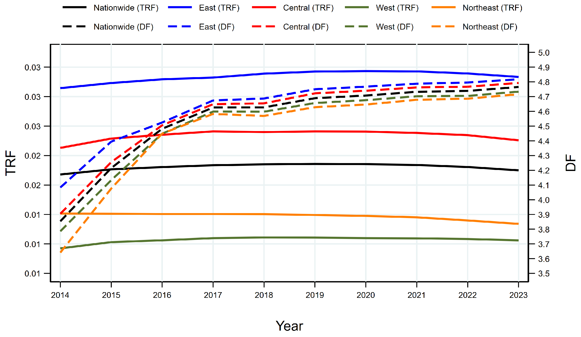
This study, as shown in Figure 2, shows that from 2014 to 2023, both TRF and DF exhibit a dynamic pattern characterized by staged growth followed by stabilization. From a national perspective, TRF shows relatively small fluctuations: a gradual increase from 2014 to 2019, followed by a slight decline, and its marginal growth tends to converge. In contrast, DF experienced a leapfrog growth during 2014–2017 and then entered a stable stage. It is worth noting that the magnitude of improvement in DF is significantly greater than that in TRF, indicating that DF has greater expansion capacity in terms of coverage breadth. In contrast, TRF is more reflected in structural adjustments of existing stock.

From the regional perspective, the development of TRF exhibits strong path dependence. The eastern region has long maintained a high level, and the central region remains relatively stable. In contrast, the western and northeastern regions show limited improvement and a slight decline in the later period. In contrast, during 2014–2016, DF rapidly diffused due to technological advantages, significantly narrowing regional disparities. However, after 2016, its growth began to show structural divergence: the eastern region continued to maintain its leading position and accelerated expansion, while growth rates in the central, western, and northeastern regions slowed, leading to a re-expansion of regional disparities and the re-emergence of the digital divide.

Meanwhile, the development of DF has led to significant crowding out of TRF. With DF’s continued penetration into areas such as payments and credit, it gradually replaces some TRF functions through greater efficiency and lower information-acquisition costs, leading to a slowdown in TRF’s growth after 2016. This, to some extent, reflects the transformation of China’s rural financial system from being dominated by traditional finance to being driven by DF.

4.1.2. Temporal Evolution Characteristics of AER

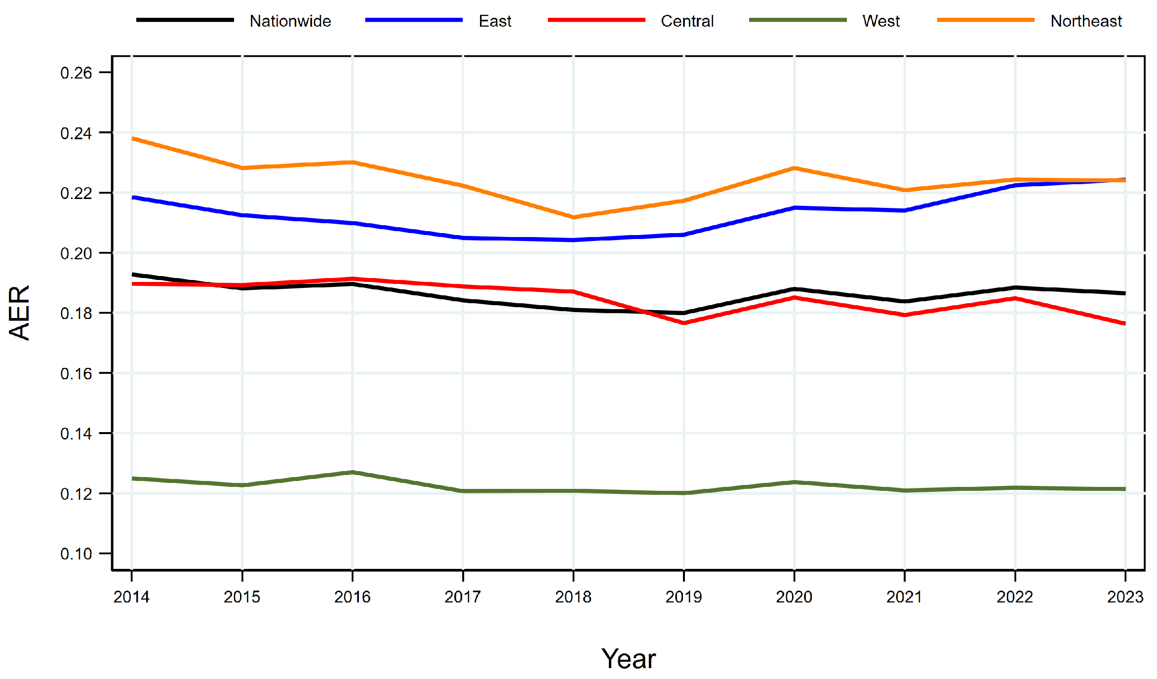
As shown in Figure 3, from 2014 to 2023, AER at the national level exhibits clear stage-based fluctuation characteristics. Overall, AER follows a U-shaped trajectory, first declining and then rebounding. This indicates that the agricultural system is highly sensitive and easily affected by uncertainties, yet possesses the capacity for gradual recovery and adjustment. From the regional distribution, AER shows significant spatial heterogeneity. The northeastern region remains at a relatively high level for a long period, followed by the eastern region. In contrast, the central and western regions are relatively lower, with the western region consistently at the lowest level. Overall, the pattern presents as “Northeast > East > Central > West.”

4.2. Baseline Regression Analysis

Based on the aforementioned optimal algorithm selection method, this section uses random forest and gradient boosting algorithms to compute the MSE of Equations (1) and (2). As shown in

Table 3. Comparison of MSE between RF and GB algorithms.

Algorithm	MSE_Y	MSE_D
RF	0.031	0.000
GB	0.032	0.001
First-order control terms	YES	YES
Second-order control terms	YES	YES
Year FE	YES	YES
County FE	YES	YES
N	14,100	14,100

Note(s): MSE_Y and MSE_D represent the cross-validation errors of the DML model for Equations (1) and (2), respectively; RF and GB denote the algorithms Random Forest and Gradient Boosting, respectively.

, the random forest algorithm yields the smallest MSE in both Equations (1) and (2). Therefore, based on Equation (7), the random forest algorithm is identified as the optimal algorithm combination for Equations (1) and (2), and regression analysis is conducted accordingly. The results are reported in

Table 4. Baseline regression results based on RF algorithm.

Variable	(1)	(2)	(3)	(4)	(5)
	AER	AER	Resistance	Recovery	Adaptability
TRF	0.324 ***	0.328 ***	0.166 ***	0.084 ***	0.184 ***
	(0.098)	(0.097)	(0.039)	(0.028)	(0.064)
First-order control terms	YES	YES	YES	YES	YES
Second-order control terms	NO	YES	YES	YES	YES
Year FE	YES	YES	YES	YES	YES
County FE	YES	YES	YES	YES	YES
N	14,100	14,100	14,100	14,100	14,100

Note(s): *** indicate significance at the 1% level, respectively, with robust standard errors in parentheses. The table is the same as the one below.

, where Column (1) controls for the linear terms of control variables, time fixed effects, and county fixed effects over the full sample period, while Column (2) further includes the squared terms of control variables. The results show that the coefficients in Columns (1) and (2) are both positive and statistically significant at the 1% level, indicating that TRF significantly enhances AER and validating H1.

To further examine the specific effects of TRF on the three dimensions of AER, Columns (3)–(5) in Table 4 report the regression results for resistance capacity, recovery capacity, and adaptability capacity, respectively. The results show that all coefficients are significantly positive at the 1% level, indicating that TRF exerts a significant promoting effect on all three dimensions of AER. Given that the RF algorithm can automatically capture nonlinear relationships and complex interaction effects among variables by integrating a large number of decision trees, it substantially relaxes the stringent assumptions of linear models, thereby reducing the risk of model specification bias and improving prediction stability. Moreover, according to the optimal algorithm selection results, RF achieves the lowest MSE in both the main and auxiliary equations. Therefore, the subsequent analysis primarily relies on the RF algorithm for regression estimation.

In addition, to further verify the robustness of the above results, four commonly used algorithms—Lasso regression (LASSO), elastic net (EN), support vector machine (SVM), and neural network (NN)—are added on the basis of the RF and GB algorithms. The newly selected optimal algorithm combination is SVM and RF, and regression analysis is conducted accordingly. The results are shown in

Table 5. Baseline regression results based on SVM and RF algorithm.

Variable	(1)	(2)	(3)	(4)	(5)
	AER	AER	Resistance	Recovery	Adaptability
TRF	0.531 ***	0.565 ***	0.244 ***	0.147 ***	0.119 *
	(0.121)	(0.135)	(0.065)	(0.047)	(0.071)
First-order control terms	YES	YES	YES	YES	YES
Second-order control terms	NO	YES	YES	YES	YES
Year FE	YES	YES	YES	YES	YES
County FE	YES	YES	YES	YES	YES
N	14,100	14,100	14,100	14,100	14,100

Note(s): *, *** indicate significance at the 10% and 1% levels, respectively, with robust standard errors in parentheses. The table is the same as the one below.

. The impact of TRF on AER and its three dimensions remains significantly positive, consistent with the baseline regression results, thereby confirming the robustness of the baseline findings.

4.3. Robustness Checks

This study conducts eight robustness checks on the baseline regression model. As shown in

Table 6. Additional robustness test results.

Variable	(1)	(2)	(3)					(4)
	Adjusted Folds		Adjust the DML Algorithms					TWFE
	K = 3	K = 8	LASSO	EN	GB	NN	SVM
TRF	0.323 ***	0.291 ***	0.122 ***	0.122 ***	0.189 ***	0.071 ***	0.716 ***	0.173 ***
	(0.084)	(0.089)	(0.043)	(0.043)	(0.052)	(0.023)	(0.044)	(0.051)
Control variables	YES	YES	YES	YES	YES	YES	YES	YES
Year FE	YES	YES	YES	YES	YES	YES	YES	YES
County FE	YES	YES	YES	YES	YES	YES	YES	YES
N	14,100	14,100	14,100	14,100	14,100	14,100	14,100	14,100

Note(s): LASSO, EN, GB, NN, and SVM denote the algorithms LASSO, elastic net, gradient boosting, neural network, and support vector machine, respectively; *** indicates significance at the 1% levels, respectively, with robust standard errors in parentheses. The table is the same as the one below.

and

Table 7. Robustness test results.

Variable	(1)	(2)	(3)	(4)		(5)	(6)
	1% Wins-Orization	5% Wins-Orization	City–Year FE	Core var. ($\mathit{t}\mathbf{-}\mathbf{1}$)	Controls ($\mathit{t}\mathbf{-}\mathbf{1}$)	Excluding Other FIs	Replace Explanatory Variable	Replace Dependent Variable
TRF	0.528 ***	0.582 ***	0.332 ***		0.388 ***	0.328 ***		0.278 ***
	(0.070)	(0.089)	(0.090)		(0.068)	(0.097)		(0.092)
Lagged TRF				0.261 ***
				(0.073)
ln(AgriLoan+1)							0.010 ***
							(0.003)
Control variables	YES	YES	YES	YES	YES	YES	YES	YES
Year FE	YES	YES	YES	YES	YES	YES	YES	YES
County FE	YES	YES	YES	YES	YES	YES	YES	YES
N	14,100	14,100	14,100	12,690	12,690	14,100	14,100	14,100

Note(s): *** indicates significance at the 1% level, respectively, with robust standard errors in parentheses. The table is the same as the one below.

, first, the model fitting method is adjusted by changing the number of cross-fitting folds in the DML framework from the baseline 5-fold setting to 4-fold and 8-fold, respectively, and re-estimating the model. Second, the machine learning algorithms are adjusted by replacing the RF used in the baseline regression with five alternative algorithms, including Lasso regression, EN, GB, NN, and SVM, to validate the robustness of the baseline results across different algorithms. Third, a TWFE model is introduced, and the baseline regression is re-estimated using a conventional TWFE specification. Fourth, the influence of outliers is addressed by winsorizing all variables at the 1% and 5% levels and re-estimating the model. Fifth, interaction fixed effects are introduced by adding city-by-time interactions to the baseline model to control for time-varying heterogeneity across cities. Sixth, a one-period lag specification is applied, lagging both the core explanatory variable and the control variables by one period. Seventh, the potential confounding effects of other financial institutions are controlled for by collecting data on the number of outlets of other financial institutions, standardizing them by county administrative area, and including them as control variables. Eighth, both the explanatory and dependent variables are replaced: the TRF variable is replaced by the logarithm of agricultural loan amounts at the county level, and the AER index is recalculated using the equal-weighting method and used as the new dependent variable in the regression.

4.4. Endogeneity Treatment

Although this study has controlled for factors affecting AER as comprehensively as possible in the baseline regression, endogeneity may still arise due to omitted variables or measurement errors. Therefore, this section further addresses the potential endogeneity issue by employing an instrumental variable (IV) approach. Following the approach of [45]. the average number of rural financial institutions in other counties within the same prefecture-level city in the same year is used as the IV. This IV satisfies both the relevance and exogeneity conditions. On the one hand, compared with counties in other cities, counties within the same prefecture-level city generally share more similar characteristics in terms of economic development, historical background, and cultural context, resulting in relatively similar levels of TRF development. On the other hand, credit financing is typically characterized by geographical segmentation [46]. particularly evident in the lending activities of rural financial institutions in China. The most direct manifestation is that the establishment and operation of rural financial institutions in China are not primarily market-driven but are, to a considerable extent, policy-oriented. The principal function of these institutions is to “take root in counties and serve local communities,” thereby supporting the implementation of national policy arrangements. As a result, the lending activities of rural financial institutions are largely confined to their own counties, making it difficult for them to exert a substantive cross-county impact on AER. This is also consistent with Stiglitz’s theory of imperfect information and imperfect competition in rural financial markets in developing countries.

Additionally, to enhance the robustness of the empirical findings, this study further introduces a second instrumental variable to address endogeneity. Specifically, the natural logarithm of one plus the average number of rural financial institution branches at the county level during 1996–2005 is constructed as an alternative instrumental variable. This instrumental variable satisfies both the relevance and exclusion restrictions. Regarding relevance, the historical distribution of rural financial institution branches in China exhibits strong path dependence. Counties with higher branch density in earlier periods accumulated more developed financial infrastructure, deeper client relationships, and richer credit experience. Under institutional inertia, these advantages continuously reinforce TRF’s current supply capacity, thereby ensuring a strong correlation between the instrumental variable and the core explanatory variable. Regarding the exclusion restriction, the spatial distribution of rural financial institution branches during 1996–2005 was primarily determined by administrative allocation inherited from the planned economy system. For example, the Agricultural Bank of China established county-level branches and Rural Credit Cooperatives set up township-level outlets in accordance with state-directed financial resource allocation rather than market-based responses to county-level agricultural economic potential. Moreover, the construction period of this instrumental variable is at least nine years prior to the sample period (2014–2023). During this interval, China’s rural financial system underwent a series of institutional reforms, including the 2006 incremental reform of rural finance and the establishment of village and township banks in 2007. As a result, the direct channels through which historical rural financial branch distribution could affect current agricultural economic resilience have been largely severed.

Based on this, and following Chernozhukov et al. [32]. A partially linear IV model within the DML framework is constructed as follows:

$$AE{R}_{it}={\theta }_{0}TR{F}_{it}+g\left(X_{it}\right)+U_{it}$$

(10)

$$I{V}_{it}=m\left(X_{it}\right)+V_{it}$$

(11)

Equation (11) is an instrumental variable regression equation, $I{V}_{it}$ is the IV, and the definitions of the other variables are the same as in Equations (1) and (2).

It is worth noting that the IV approach adopted in this section is methodologically innovative. Specifically, it not only integrates the DML framework with the traditional two-stage least squares (2SLS) method, but also follows the idea of an “optimal algorithm combination,” whereby cross-fitting in DML is used to compute the MSE and identify the optimal set of algorithms, which is then applied in the subsequent 2SLS estimation. More specifically, the optimal algorithm combination is first determined based on the selection procedure used in the baseline regression. Second, the study uses DML to remove the effects of control variables on $AE{R}_{it}$, $TR{F}_{it}$, and $I{V}_{it}$. Finally, the 2SLS method is employed for estimation.

Table 8. IV regression results based on GB algorithm.

Variable	(1)	(2)	(3)	(4)
	First Stage	Second Stage	First Stage	Second Stage
	TRF	AER	TRF	AER
IV1: avg. rural financial institutions in other counties (prefecture-level)	1.187 ***
	(0.015)
TRF		1.702 ***
		(0.034)
IV2: Ln (Average Number of Historical Rural Financial Institution Outlets per County + 1) (1996–2005)			0.011 ***
			(0.001)
TRF				3.066 ***
				(0.349)
Underidentification test: Kleibergen-Paap rk LM statistic		2111.688		73.079
(p-value)		(0.0000)		(0.0000)
Weak identification test: Cragg-Donald Wald F statistic		30,930.880		93.866
Endogeneity test: ${\chi }^2\left(1\right)$ statistic		149.169		59.405
(p-value)		(0.0000)		(0.0000)
Control variables	YES	YES	YES	YES
Year FE	YES	YES	YES	YES
County FE	YES	YES	YES	YES
N	14,100	14,100	14,100	14,100

Note(s): *** denotes significance at the 1% level. Values in parentheses are robust standard errors, unless p-values from the underidentification and endogeneity tests (shown in brackets).

reports the 2SLS regression results using two instrumental variables. Columns (1) and (3) present the first-stage results, where both instrumental variables exhibit a statistically significant positive effect on TRF at the 1% significance level, indicating that the relevance assumption is satisfied. Columns (2) and (4) report the second-stage results, showing that TRF has a significantly positive impact on AER. After addressing endogeneity using the two instrumental variables, the estimated results remain consistent with those of the baseline regression.

Admittedly, counties within the same prefecture-level city often share similar agricultural policy environments or face comparable natural disaster risks, both of which may directly affect AER. Therefore, to demonstrate that the IV satisfies the exclusion restriction, this section conducts an indirect test of the exogeneity of the IV, namely, the average number of rural financial institutions in other counties within the same prefecture-level city. Specifically, following the approach of Liu et al. [47]. this study examines whether the IV affects AER in regions where its first-stage relevance is weak. If the IV satisfies the exclusion restriction, its impact on AER should be weak or disappear altogether in areas with low first-stage correlation. Conversely, if the IV remains highly correlated with AER in these areas, this would suggest that it is likely affecting AER through channels other than TRF. Based on this logic, this study conducts a reduced-form regression using a subsample of counties with average numbers of rural financial institutions below the 25th percentile in the same prefecture-level city. As reported in

Table 9. IV exclusion restriction test.

Variable	Bottom 25th Percentile AER
IV: avg. rural financial institutions in other counties (prefecture-level)	−0.000
	(0.002)
Control variables	YES
Year FE	YES
County FE	YES
N	3525

Note(s): Robust standard errors in parentheses. The table is the same as the one below.

, the estimated coefficient is very small and statistically insignificant, indicating that the IV is unlikely to affect AER through channels other than TRF.

4.5. Mediation Mechanism Analysis

Although the baseline regression has empirically demonstrated that TRF significantly enhances AER, and a series of robustness and endogeneity checks further confirm the stability of this conclusion, the specific transmission channels proposed in the theoretical framework have not yet been empirically verified. In this section, we continue to employ the DML approach to construct econometric models and examine the effects of TRF on the proposed mechanism variables, thereby investigating whether TRF enhances AER through stimulating agricultural technological innovation and promoting agricultural socialized services, and testing hypotheses H2a and H2b.

4.5.1. Stimulating Agricultural Technological Innovation

As shown in column (2) of

Table 10. Results of the mediation mechanism test.

Variable	ATI Mediation Mechanism			ASS Mediation Mechanism
	(1)	(2)	(3)	(4)	(5)	(6)
	AER	ATI	AER	AER	ASS	AER
TRF	0.328 ***	6.819 **	0.299 ***	0.328 ***	2.926 **	0.307 ***
	(0.097)	(2.977)	(0.075)	(0.097)	(1.480)	(0.103)
ATI			0.004 ***
			(0.000)
ASS						0.007 ***
						(0.000)
Control variables	YES	YES	YES	YES	YES	YES
Year FE	YES	YES	YES	YES	YES	YES
County FE	YES	YES	YES	YES	YES	YES
N	14,100	14,100	14,100	14,100	14,100	14,100

Note(s): **, *** indicate significance at the 5%, and 1% levels, respectively, with robust standard errors in parentheses. The table is the same as the one below.

, TRF has a coefficient of 6.819 on agricultural technological innovation and is statistically significant at the 5% level, indicating that TRF development can provide financial support for agricultural R&D and effectively promote the improvement of agricultural technological innovation. Column (3), based on column (1), includes the mediator variable (ATI). The coefficient of TRF on AER decreases to 0.299, while the coefficient of agricultural technological innovation on AER is 0.004 and statistically significant. This suggests that agricultural technological innovation plays a partial mediating role, with the mediating effect accounting for 8.23% of the total effect; therefore, Hypothesis H2a is validated.

4.5.2. Promoting Agricultural Socialized Services

As shown in column (5) of Table 10, TRF has a coefficient of 2.926 on agricultural socialized services (ASS) and is statistically significant at the 5% level, indicating that TRF development can effectively promote the improvement of agricultural socialized service capacity. Column (6), based on column (4), includes the mediator variable (ASS). The coefficient of TRF on AER decreases to 0.307, while the coefficient of agricultural socialized services on AER is 0.007 and statistically significant. This suggests that agricultural socialized services play a partial mediating role, with the mediating effect accounting for 6.1% of the total effect; therefore, Hypothesis H2b is validated.

4.6. Threshold Effect Analysis

4.6.1. Existence Test

Based on the theoretical analysis above, the impact of TRF on AER exhibits nonlinear threshold behaviour that varies with DF’s development level. Following Equation (9), we sequentially test the single-threshold, double-threshold, and triple-threshold effects.

Table 11. Threshold effect: significance test and CIs (bs = 500).

Threshold Variable	Threshold Count	F-Value	10%	5%	1%	Threshold Value	95% CIs
DF	Single threshold	55.29 ***	15.99	19.67	26.08	4.1501 ***	[4.1295, 4.1608]
	Double threshold	10.98	15.25	19.20	24.52	4.52	—
DF breadth	Single threshold	76.84 ***	14.56	16.89	24.38	4.4653 ***	[4.4638, 4.4662]
	Double threshold	14.35 *	12.82	14.36	18.60	4.4653 *	[4.4614, 4.4662]
						4.5024 *	[4.4962, 4.5031]
	Triple threshold	10.75	19.15	22.34	29.37	—	—
DF depth	Single threshold	97.75 ***	17.03	19.75	24.39	3.9697 ***	[3.9453, 3.9882]
	Double threshold	19.04 **	15.76	18.76	27.86	3.9697 **	[3.9453, 3.9882]
						4.5086 **	[4.4447, 4.5145]
	Triple threshold	16.28	29.93	34.96	44.18	—	—
DF digitalization	Single threshold	21.89 **	16.84	19.39	26.84	4.0762 **	[4.0519, 4.0831]
	Double threshold	3.17	13.44	16.92	20.41	—	—

Note(s): *, **, *** indicate significance at the 10%, 5%, and 1% levels, respectively. F-stats and critical values (10%, 5%, 1% sig. levels) are from 500 bootstrap replications. CIs denote confidence intervals.

reports the threshold significance tests, estimated threshold values, and corresponding confidence intervals for DF and its three dimensions (coverage breadth, usage depth, and degree of digitalization). The results show that DF and its degree of digitalization exhibit a single-threshold effect, but no double-threshold effect is found. In contrast, the coverage breadth and usage depth of DF exhibit both single- and double-threshold effects, while no triple-threshold effect is detected.

4.6.2. Test Results

As shown in

Table 12. Threshold effect results.

Variable	(1)	(2)	(3)	(4)
	DF	DF Breadth	DF Depth	DF Digitalization
First threshold estimate	4.1501 ***	4.4653 *	3.9697 **	4.0762 **
Second threshold estimate	—	4.5024 *	4.5086 **	—
$TR{F}_{it}I(q_{it}\le {\gamma }_1)$	0.293 ***	0.259 ***	0.476 ***	0.175 ***
	(0.048)	(0.043)	(0.056)	(0.042)
$TR{F}_{it}I({\gamma }_1<q_{it}\le {\gamma }_2)$	—	0.157 ***	0.163 ***	—
	—	(0.044)	(0.041)	—
$TR{F}_{it}I(q_{it}>{\gamma }_2)$	0.097 **	0.076 **	0.095 **	0.092 **
	(0.039)	(0.039)	(0.039)	(0.039)
Control variables	YES	YES	YES	YES
Year FE	YES	YES	YES	YES
County FE	YES	YES	YES	YES
N	14,100	14,100	14,100	14,100

Note(s): *, **, *** indicate significance at the 10%, 5%, and 1% levels, respectively. F-stats and critical values (10%, 5%, 1% sig. levels) are from 500 bootstrap replications. CIs denote confidence intervals.

, the impact of TRF development on AER differs significantly across different levels of DF and its dimensions. As the development level of DF and its dimensions increases, the positive effect of TRF development on AER gradually weakens. Taking DF as an example, when the level of DF is below the first threshold value, the regression coefficient of TRF is 0.293; after crossing the threshold value, the coefficient declines to 0.097. Similarly, across different threshold intervals of coverage breadth, usage depth, and degree of digitalization, the effect coefficient of TRF gradually decreases as the development level of these dimensions increases, thereby validating Hypothesis H3. A possible explanation is that, by leveraging its technological advantages, DF breaks geographical constraints and provides agricultural business entities with more diversified and convenient financing channels through expanding financial service coverage and enriching financial product offerings, thereby reducing their dependence on rural financial institutions. However, the regression coefficients of TRF remain significantly positive at least at the 5% level across all threshold intervals, indicating that TRF continues to be an important force in enhancing AER. Therefore, efforts should be made to promote the coordinated development of DF and TRF and to build a multi-level rural financial service system, thereby ensuring that agricultural business entities can access high-quality financial services.

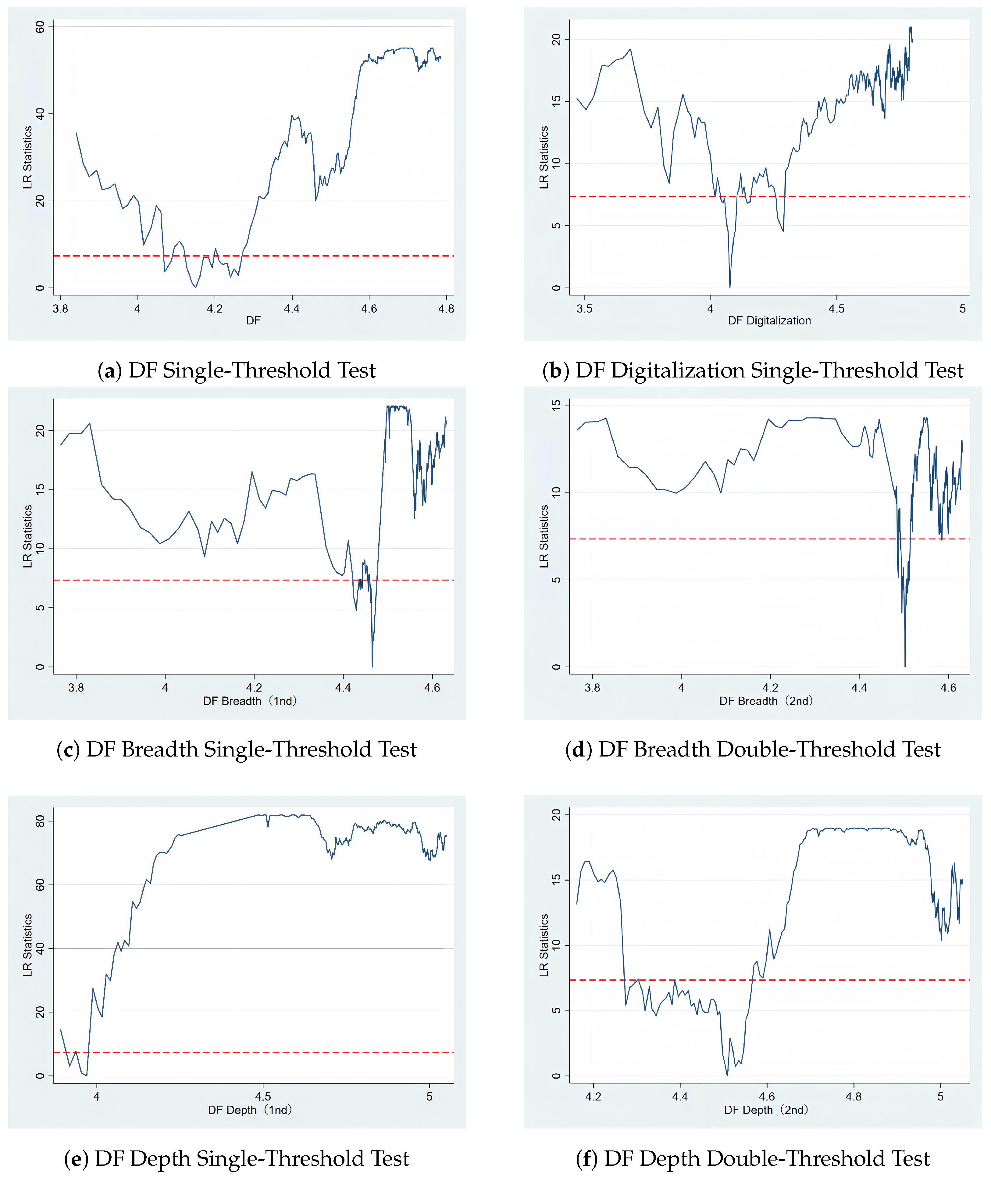
In addition, we present the threshold effect test figures to provide a more intuitive illustration of the significance of the threshold effects. As shown in Panels a–f of Figure 4, in both the single-threshold and double-threshold tests for DF and its dimensions—coverage breadth, usage depth, and degree of digitalization—the LR statistics in most intervals are substantially higher than the critical values (dashed lines), indicating significant threshold effects.

4.6.3. Robustness Test of Threshold Effects and Endogeneity Treatment

For panel threshold models, some studies employ the dynamic panel threshold model proposed by Seo and Shin [48]. to alleviate endogeneity concerns. However, this model cannot estimate multiple-threshold specifications. In reality, the relationship between DF and TRF is often dynamic and evolving. Applying a dynamic panel threshold model may overlook the existence of multiple thresholds and thus fail to reflect actual conditions, making it unsuitable for this study. Therefore, to ensure the robustness of the baseline threshold regression results, and following the approach of Ye et al. [49]. we use the composite AER index calculated by the equal-weighting method as a new dependent variable for robustness testing, thereby enhancing the reliability of the findings. The results are reported in

Table 13. Robustness test of threshold effects by replacing the dependent variable.

Variable	(1)	(2)	(3)	(4)
	DF	DF Breadth	DF Depth	DF Digitalization
First threshold estimate	3.9082 ***	4.0305 ***	3.9697 ***	4.2887 ***
Second threshold estimate	4.7640 ***	—	5.0320 ***	4.7870 ***
$TR{F}_{it}I(q_{it}\le {\gamma }_1)$	0.302 ***	0.230 ***	0.376 ***	0.156 ***
	(0.056)	(0.053)	(0.058)	(0.042)
$TR{F}_{it}I({\gamma }_1<q_{it}\le {\gamma }_2)$	0.100 ***	—	0.113 ***	0.081 **
	(0.040)	—	(0.040)	(0.040)
$TR{F}_{it}I(q_{it}>{\gamma }_2)$	−0.012	0.063	0.003	−0.036
	(0.041)	(0.040)	(0.041)	(0.041)
Control variables	YES	YES	YES	YES
Year FE	YES	YES	YES	YES
County FE	YES	YES	YES	YES
N	14,100	14,100	14,100	14,100

Note(s): **, *** indicate significance at the 5%, and 1% levels, respectively. F-stats and critical values (10%, 5%, 1% sig. levels) are from 500 bootstrap replications. CIs denote confidence intervals.

. It can be seen that, as the level of DF and its dimensions increases, the effect coefficient of TRF on AER gradually declines, becomes statistically insignificant, and even turns negative in some cases. These findings are consistent with the conclusions obtained from the baseline threshold regressions.

Additionally, Regarding endogeneity treatment, this section further employs two approaches based on the first instrumental variable in this study. First, following Wooldridge [50]. the endogeneity of each threshold variable is addressed using an IV approach before conducting the threshold effect analysis. Specifically, in the first stage, each threshold variable is regressed on the instrumental variable (IV), and the resulting residuals are then included as additional control variables in the panel threshold model. This procedure removes the endogenous component of the threshold variables from the error term, thereby ensuring the consistency of the threshold estimates. The regression results are reported in Table S2 of Supplementary Materials A. Overall, as DF increases, the estimated coefficients of TRF on AER decrease, indicating a diminishing marginal effect, consistent with the main findings of this study. Second, following Feng Yongqi et al. [51]. the threshold values are first estimated using the panel threshold model. The sample is then divided into subgroups according to the estimated threshold values, and IV regressions are conducted within each subsample. Specifically, based on the threshold values of DF and its three dimensions identified above, the sample is divided into two or three groups (two groups for a single threshold and three groups for double thresholds). This allows for an endogeneity-robust examination of the effect of TRF on AER under different levels of DF. As shown in Tables S3–S6 in Supplementary Materials B, the results indicate that as DF and its dimensions increase, the estimated coefficients of TRF on AER decline, demonstrating a clear diminishing marginal effect, consistent with the main conclusions of this study.

4.6.4. Interaction Term Analysis

The diminishing marginal effect of TRF on AER may also be driven by the fact that regions with higher levels of DF tend to possess a more developed financial ecosystem. Therefore, to further test Hypothesis H3, this section introduces interaction terms for analysis. In addition, to avoid multicollinearity, TRF and DF as well as their respective dimension indicators are first mean-centered before constructing the interaction terms for regression analysis. As shown in

Table 14. Interaction term analysis.

Variable	(1)	(2)	(3)	(4)
	AER	AER	AER	AER
TRF_DFII	−0.171 ***
	(0.052)
TRF_Breadth		−0.176 ***
		(0.061)
TRF_Depth			−0.102 ***
			(0.037)
TRF_Digitization				−0.043 *
				(0.022)
Control variables	YES	YES	YES	YES
Year FE	YES	YES	YES	YES
County FE	YES	YES	YES	YES
N	14,100	14,100	14,100	14,100

Note(s): *, *** indicate significance at the 10% and 1% levels, respectively, with robust standard errors in parentheses. The table is the same as the one below.

, the results indicate that the coefficients of all interaction terms are statistically significant at least at the 10% level and are consistently negative. This suggests that, with the development of DF, the promoting effect of TRF on AER weakens, indicating a “competitive crowding-out effect” between the two. This finding is also consistent with the results of the threshold effect analysis; therefore, Hypothesis H3 is further validated.

Additionally, to further enhance the robustness of the conclusions, this section controls for regional time trends and conducts interaction term analysis. The results are reported in Supplementary Materials C. The coefficients of the interaction terms across all specifications remain negative and statistically significant at the 1% level, further supporting the findings of this study: DF and TRF exhibit a competitive crowding-out effect on AER.

5. Heterogeneity Analysis

5.1. Regional Heterogeneity

To examine the heterogeneous effects of TRF on AER, the full sample is divided into four regions—eastern, central, western, and northeastern China—for separate regressions. As shown in Columns (1) of

Table 15. Heterogeneity analysis.

Variable	(1)				(2)
	Eastern	Central	Western	Northeastern	Agricultural Counties	Industrial Counties
TRF	0.229 ***	0.361 ***	0.192 ***	0.282	0.594 ***	0.191 *
	(0.074)	(0.131)	(0.041)	(0.291)	(0.102)	(0.089)
Control variables	YES	YES	YES	YES	YES	YES
Year FE	YES	YES	YES	YES	YES	YES
County FE	YES	YES	YES	YES	YES	YES
N	3300	3150	6530	1120	10,970	3130

Note(s): *, *** indicate significance at the 10% and 1% levels, respectively, with robust standard errors in parentheses. The table is the same as the one below.

, the results indicate that, except for the northeastern region, TRF has a significantly positive impact on AER at the 1% significance level in the other three regions, with the effect exhibiting a clear gradient pattern of “central > eastern > western.”

Possible explanations are as follows. First, in the central region, where household-based farming dominates, farmers generally lack effective collateral and credit records, making it difficult for them to obtain credit from large commercial banks. Rural financial institutions, however, leverage their geographical proximity to acquire farmers’ soft information, enabling better credit assessment and differentiated financial services, thereby significantly enhancing AER. Second, in the eastern region, agriculture accounts for a relatively small share of the economy, and the industrial structure is highly diversified; agricultural operators are therefore less dependent on rural financial institutions, leading to a weaker supporting role. Third, although the western region faces harsh natural conditions and weak agricultural infrastructure, with limited non-farm employment opportunities, rural financial institutions remain a key financial support for agricultural operators in coping with uncertainty shocks. However, due to relatively underdeveloped rural financial systems and limited service coverage, the effectiveness of financial support remains weak. Finally, the northeastern region is dominated by state-owned farms and large agricultural enterprises, which enjoy high creditworthiness and easier access to funding from large commercial banks. Moreover, AER in this region is relatively high, and dependence on rural financial institutions is limited.

To verify the validity of the explanation for the heterogeneity in Northeast China, this study follows Wang Xiuhua and Peng Derong [52] by using the number of agricultural enterprises with registered capital of RMB 10 million or above as a proxy for state-owned farms and large agricultural enterprises (hereinafter referred to as “agricultural enterprise count”). Based on the median value of agricultural enterprise count, the full sample is divided into a high-agricultural-enterprise group and a low-agricultural-enterprise group to separately examine the impact of TRF on AER, as shown in Supplementary Materials D. The results indicate that in counties with a high number of agricultural enterprises, the effect of TRF on AER is positive but not statistically significant, whereas in counties with a low number of agricultural enterprises, the estimated coefficient of TRF on AER is positive and statistically significant at the 5% level. This finding, to some extent, validates the rationality of the heterogeneity explanation for Northeast China.

5.2. Agricultural vs. Industrial Counties Heterogeneity

Differences in county-level economic orientation lead to variations in financial resource allocation, which may, in turn, generate significant differences in productivity. Following Sun et al. [28], the sample is divided into agricultural counties and industrial counties (i.e., county-level cities) based on whether a county is designated as a county-level city.

As shown in Columns (2) of Table 15, the positive effect of rural financial institutions on AER is significantly stronger in agricultural counties than in industrial counties. A possible explanation is that agricultural counties are dominated by the agricultural sector, with a larger number of agricultural operators and strong credit demand rigidity. In contrast, industrial counties are dominated by industrial activities, where credit resources are primarily allocated to the industrial sector, while agricultural production is relatively fragmented. This increases the lending costs of rural financial institutions and reduces their incentives to provide agricultural credit, thereby weakening their supporting effect on agriculture.

6. Further Discussion

6.1. Relative Disparities in Agricultural Development

The preceding analysis has verified that TRF development can significantly enhance AER. However, in the digital era, what roles do TRF and DF play in narrowing regional disparities in agricultural development? To address this question, this section draws on the research framework of Xie et al. [53]. and constructs the following spatial coordination effect model to examine whether TRF and DF can reduce regional disparities in agricultural development and promote coordinated regional development.

$${\displaystyle \frac{Y_{it}}{Y_{mt}}}={\theta }_{it}TR{F}_{it}+g\left(X_{it}\right)+U_{it},E\left(U_{it}\right|TR{F}_{it},X_{it})=0$$

(12)

$$TR{F}_{it}=m\left(X_{it}\right)+V_{it},E\left(V_{it}\right|X_{it})=0$$

(13)

$${\displaystyle \frac{Y_{it}}{Y_{mt}}}={\theta }_{it}D{F}_{it}+g\left(X_{it}\right)+U_{it},E\left(U_{it}\right|D{F}_{it},X_{it})=0$$

(14)

$$D{F}_{it}=m\left(X_{it}\right)+V_{it},E\left(V_{it}\right|X_{it})=0$$

(15)

where $Y_{it}$ denotes the county-level AER, and $Y_{mt}$ represents the maximum value within the corresponding regional AER set. The ratio of $Y_{it}$ to $Y_{mt}$ is the Agricultural Development Relative Disparity Index, which measures the degree of disparity in agricultural development between regions. A value closer to 1 indicates a smaller relative disparity between the two regions, whereas a value closer to 0 indicates a larger relative disparity. The indicator constructed using this method can effectively measure the relative disparities in agricultural development among counties at the national level, among counties within major grain-producing functional regions, among counties across the four major regions, among counties in northern and southern regions, and among counties in coastal and inland regions, thereby comprehensively evaluating the regional coordination effects of TRF and DF. It should be noted that the primary objective of this section is to identify the effects of TRF and DF on relative disparities in county-level agricultural development. Therefore, the measure of agricultural development relative disparity must retain individual variation at the county level. In contrast, disparity indicators such as the Theil Index and the coefficient of variation measure disparities at the regional level and are thus not suitable for the research objective of this section.

As shown in

Table 16. Regression results for inter-regional disparities in AER.

Variable	(1)	(2)	(3)	(4)	(5)
	Inter-County Disparity	Grain Zone Disparity	Four-region Disparity	North-South Disparity	Coastal-Inland Disparity
TRF	0.653 ***	0.755 ***	0.508 ***	0.682 ***	0.586 ***
	(0.198)	(0.239)	(0.201)	(0.210)	(0.181)
DF	−0.007 **	−0.017 ***	−0.025 ***	−0.011 ***	−0.009 **
	(0.003)	(0.004)	(0.005)	(0.004)	(0.004)
Control variables	YES	YES	YES	YES	YES
Year FE	YES	YES	YES	YES	YES
County FE	YES	YES	YES	YES	YES
N	14,100	14,100	14,100	14,100	14,100

Note(s): **, *** indicate significance at the 5%, and 1% levels, respectively. In the model with DF as the core explanatory variable, the original DF controls (including its components) were replaced by the first- and second-order terms of rural financial institutions; all other controls remain unchanged.

, TRF significantly narrows regional disparities in agricultural development, and this effect is generally observed nationwide. However, overall, DF does not reduce agricultural development disparities; instead, it exacerbates them, and this effect is also prevalent across the country. Specifically, the effects of different dimensions of DF on regional disparities exhibit substantial heterogeneity. First, regarding the breadth of coverage dimension, as reported in Columns (1)–(3), DF breadth significantly enlarges agricultural development disparities across all five regional classifications, making it the most prominent dimension contributing to regional divergence. This finding suggests that the expansion of accessibility to digital financial services may be characterized by considerable spatial unevenness. Second, regarding the depth of use dimension, Columns (1) and (5) show that DF depth significantly reduces agricultural development disparities at the national level and between coastal and inland regions, whereas Column (3) indicates that it significantly enlarges disparities across the four major regions. These results suggest that, as the intensity of DF use increases, it may, to some extent, help narrow regional development gaps. Third, the degree of digitalization is insignificant across all five levels of regional disparity, indicating that improvements in digitalization have not yet generated a systematic impact on regional agricultural development disparities.

A possible explanation for this finding is as follows: According to financial geography theory, geographical proximity helps reduce information acquisition costs and improve risk assessment efficiency [54,55]. Rural financial institutions accumulate farmers’ “soft information” through long-term interactions, enabling relationship-based lending that helps alleviate regional disparities in agricultural development [20]. In contrast, DF tends to widen agricultural development gaps through both the “digital divide” and the “financial siphon” effect. On the one hand, the diffusion of DF heavily depends on internet infrastructure, digital literacy, and financial knowledge. These conditions are relatively well-developed in advanced regions such as eastern coastal areas, where farmers are more likely to access DF services, thereby further strengthening local agricultural resilience. In contrast, underdeveloped regions in central and western China face constraints such as weak digital infrastructure and low adoption capacity, limiting access to DF and resulting in a “Matthew effect” [56]. which widens regional disparities in agricultural development. On the other hand, DF facilitates highly efficient capital mobility. Combined with the inherent vulnerability of agriculture and the profit-seeking nature of financial capital, funds tend to flow toward more profitable regions or non-agricultural sectors [57,58]. This “financial siphon” effect intensifies capital outflow from financially constrained regions [59]. further widening the gap between agricultural and non-agricultural production efficiency. As this gap increases, the willingness of agricultural operators to engage in agricultural production declines [60]. thereby further exacerbating regional disparities in agricultural development.

Notably, this study finds that DF, overall, does not reduce agricultural development disparities; rather, it aggravates them to some extent. Existing studies generally argue that DF can overcome the spatial and temporal constraints of traditional financial services, reduce information asymmetry and transaction costs, improve the efficiency of financial resource allocation, and promote high-quality agricultural development across regions [61,62]. However, the inclusiveness of DF is not automatically realized and largely depends on individual and regional conditions. Research has shown that disparities in digital infrastructure, digital skills, and access to digital resources affect the effective use of DF services and may lead to an “elite capture” phenomenon, thereby weakening DF’s role in narrowing development gaps [63]. In addition, DF possesses both “digital dividend” and “digital divide” characteristics simultaneously. The benefits generated by DF are often captured first by regions with stronger digital capabilities and more favorable development foundations, whereas regions with relatively weaker digital capacities struggle to fully realize the development dividends of DF. Consequently, a “Matthew effect” may emerge [64]. widening regional disparities in agricultural development. Therefore, although DF helps reduce information asymmetry and transaction costs, its development dividends have not been distributed evenly across regions. Instead, DF may reinforce disparities in agricultural development, resulting in a phenomenon whereby “the strong become stronger, while the weak become weaker.”

Furthermore, because the relative disparity index measured with the maximum value as the benchmark may be more sensitive to extreme values, thereby affecting the reliability of the estimation results, this section also conducts a robustness test by recalculating the relative disparity index using the regional mean AER instead of the maximum value. The results, reported in

Table 17. Robustness test using alternative measures of agricultural development disparities.

Variable	(1)	(2)	(3)	(4)	(5)
	Inter-County Disparity	Grain Zone Disparity	Four-Region Disparity	North-South Disparity	Coastal-Inland Disparity
TRF	2.155 ***	1.780 ***	1.198 ***	2.183 ***	1.414 ***
	(0.641)	(0.553)	(0.433)	(0.654)	(0.414)
DF	−0.146 ***	−0.051 ***	−0.086 ***	−0.115 ***	−0.115 ***
	(0.049)	(0.005)	(0.014)	(0.045)	(0.046)
Control variables	YES	YES	YES	YES	YES
Year FE	YES	YES	YES	YES	YES
County FE	YES	YES	YES	YES	YES
N	14,100	14,100	14,100	14,100	14,100

Note(s): *** indicate significance at the 1% level. The robustness check re-estimates the relative disparity index by replacing the regional maximum value with the regional mean AER; the resulting measure is used as the dependent variable. All other specifications remain the same as in Table 16.

, show that even after changing the measurement method for relative disparity, the conclusions remain largely consistent with the above findings, indicating robustness.

6.2. Research Limitations and Future Directions

This study provides a scientific basis for improving the rural financial service system in China and other developing countries and for bridging the agricultural development gap, but certain limitations remain.

First, due to data availability constraints at the county level, this study measures agricultural technological innovation using the number of agricultural technology patent applications and measures the level of agricultural socialized services using the number of newly established agricultural operating service organizations. However, these proxies also have certain limitations. Specifically, on the one hand, although the number of patent applications can relatively well reflect the output level of agricultural technological innovation, it cannot capture differences in the quality of innovation outcomes or their actual application effects in agricultural production. Similarly, while the number of newly established agricultural operating service organizations can characterize the development of service supply, it cannot reflect service quality and efficiency. On the other hand, the relatively low proportion of mediating effects from agricultural technological innovation and agricultural socialized services indicates that the transmission mechanism through which TRF affects AER is complex, and the channels examined in this study do not fully capture the picture. Therefore, future research may leverage AI large language models or more advanced data processing technologies to obtain more diversified datasets, introduce alternative indicators that better reflect the quality of technological innovation and the actual effectiveness of services, and incorporate potential mediating variables such as agricultural insurance and infrastructure investment into the analytical framework, so as to more comprehensively reveal the underlying mechanisms through which TRF affects AER.

Second, compared with provincial- and prefecture-level data, county-level data can better reflect regional agricultural development, but it is difficult to identify the micro-level operational mechanisms within counties, including farmers’ financing behavior, agricultural technology adoption decisions, and risk response strategies. Future research can use micro-survey data of farmers to conduct more detailed studies on the internal agricultural economic mechanisms within counties, thereby deepening the micro-level understanding of how TRF affects AER.

Third, although this study adopts a cutting-edge DML method that effectively mitigates the model specification biases inherent in traditional econometric models, causal identification still relies on the assumption that all key confounding factors have been controlled for. If there exist unobserved or hard-to-quantify omitted variables, the estimation results may still be somewhat affected. Therefore, future research can leverage pilot policies, such as promoting rural inclusive finance and digital rural construction, to construct quasi-natural experiments and combine DML methods with causal identification strategies to enrich and consolidate empirical research on the relationships among TRF, DF, and AER.

Fourth, this study focuses on causal identification at the county level. However, constrained by the availability of county-level data, the analysis assumes spatial independence across counties and does not incorporate potential spillover effects of TRF and DF across neighboring counties into the analytical framework. In reality, adjacent counties may be interconnected in terms of agricultural technology diffusion, digital financial service coverage, and market competition, thereby affecting local AER through channels such as knowledge spillovers or resource competition. Therefore, future research, subject to the availability of relevant county-level data, could employ methods such as spatial DML to further investigate spatial interaction mechanisms, thereby more comprehensively revealing the spatial transmission pathways through which TRF and DF affect AER.

7. Conclusions and Policy Implications

7.1. Conclusions

Enhancing AER provides strong support for advancing rural revitalization and ensuring food security, and is of great practical significance for sustainable agricultural development. The main findings are as follows:

(1)

TRF can significantly improve AER, with agricultural technological innovation and agricultural socialized services playing mediating roles.

(2)

DF and its dimensions, including coverage breadth, usage depth, and degree of digitalization, exhibit threshold effects in the impact of TRF on AER, and as the levels of DF and its dimensions increase, the positive effect of TRF shows a diminishing marginal trend, indicating a competitive crowding-out effect between the two.

(3)

The promoting effect of TRF on AER exhibits significant heterogeneity, being stronger in agricultural counties and in the eastern, central, and western regions, following a “Central > Eastern > Western” pattern, while it is not significant in the northeastern region.

(4)

TRF significantly reduces agricultural development disparities, whereas DF overall significantly exacerbates such disparities, although its different dimensions exhibit clear heterogeneity in their effects, with coverage breadth consistently and significantly widening regional agricultural development gaps.

7.2. Policy Implications

Based on the above findings, the following policy implications are proposed:

First, most developing countries should strengthen the rural financial system and encourage the development of rural financial institutions. Governments can provide credit guarantees and tax incentives to encourage market entities to establish rural financial institutions at the county level. For institutions established in industrialized countries and less developed regions, time-limited tax exemptions may be granted, together with green-channel services for business registration and tax declaration.

Second, coordinated development between DF and TRF should be promoted to build a multi-tier rural financial service system. Specifically, (i) a farmer information-sharing platform should be established to facilitate the sharing of “soft information” held by rural financial institutions and transaction data from DF platforms, thereby alleviating information asymmetry in rural credit markets. Specifically, local governments can lead the integration of agricultural data from agricultural businesses, banks, tax authorities, and other departments to establish a unified farmer credit database. Information on farmers’ business operations and land transfers should be incorporated into dynamic management systems to improve the efficiency of credit assessment and lending decisions by rural financial institutions. (ii) Differentiated regulatory policies should be implemented, with the “outstanding balance of agriculture-supporting loans” serving as a key performance indicator for rural financial institutions and the “coverage rate of agriculture-supporting services in remote areas” serving as a key performance indicator for DF platforms. The assessment results should be linked to incentives such as agriculture-supporting relending quotas, regulatory ratings, and tax preferences. (iii) An innovative “online + offline” joint lending model should be developed, in which DF platforms are responsible for online customer acquisition and preliminary screening, while rural financial institutions undertake offline investigations and post-loan management, with both parties sharing risks and returns. Drawing on the practical experience of Zhejiang Province’s “Internet platform + rural commercial bank” model, DF platforms can use payment records, e-commerce transaction data, and other information for online customer acquisition and credit evaluation, while rural commercial banks conduct field investigations and post-loan monitoring. This approach can fully leverage the data advantages of DF platforms and the localized service advantages of rural financial institutions, thereby improving the efficiency of rural financial services.

Third, given that the promoting effect of TRF on AER is not significant in Northeast China, efforts should focus on coordinating the optimization of financial resource allocation with the development of a modern agricultural system that aligns with the region’s agricultural operating characteristics and financial demand structure. Specifically, (i) a diversified agricultural financing system should be improved to better align financial resources with modern agricultural development. Large commercial banks and policy banks should be encouraged to establish long-term and stable financing partnerships with agricultural business entities, with priority given to supporting high-standard farmland construction, smart agriculture, and agricultural product processing industries, thereby directing more financial resources toward agricultural modernization. (ii) Financial products and service models should be innovated around the needs of large-scale agricultural operations. Given the financing characteristics of modern agricultural business entities, financing models based on agricultural orders, warehouse receipts, agricultural machinery and equipment, and land management rights should be actively explored to broaden financing channels and strengthen the risk-resistance of the agricultural economic system. (iii) Coordinated development between DF and traditional finance should be promoted to improve the efficiency of rural financial resource allocation. In response to challenges such as population outflow and rural population aging in Northeast China, the advantages of DF in information acquisition, risk identification, and targeted service provision should be fully utilized. Technologies such as digital risk control, agricultural big data, and intelligent credit services can be employed to optimize financial resource allocation and enhance the endogenous resilience and sustainable development capacity of the modern agricultural system in the region.

Fourth, attention should be paid to the “digital divide” and “financial siphon” effects to prevent the widening of agricultural development disparities. Since DF and its dimensions of coverage breadth and usage depth generally exacerbate agricultural development disparities, priority should be given to strengthening digital infrastructure construction and farmer education and training in less developed regions. By improving digital infrastructure and enhancing the financial literacy and digital application capabilities of agricultural business entities, policymakers can prevent “digital dividends” from evolving into a “digital divide.” Meanwhile, institutional arrangements for DF support for agriculture should be actively explored, and regulatory mechanisms governing capital flows between DF platforms and rural financial institutions should be strengthened to prevent excessive diversion of funds from the agricultural sector.

7.3. Supplementary Note

Based on the “Financial License Institution Code Compilation Rules (Trial)” published by the former China Banking Regulatory Commission, this study organizes data from 17 types of financial institutions, including rural commercial banks, rural cooperative banks, rural credit cooperatives, mutual aid societies, village and township banks, loan companies, state-owned commercial banks, policy banks, other commercial banks, urban credit cooperatives, trust companies, automobile finance companies, financial leasing companies, financial asset management companies, money brokerage companies, financial companies, and other types of financial institutions. “Other FIs” refers to the remaining 9 types of financial institutions excluding the first 6 types of rural financial institutions, state-owned commercial banks, and policy banks.

Since data on agricultural loan amounts at both the county and prefecture levels are not publicly available, this study follows the approach of Huang et al. [20]. Specifically, the county-level agricultural loan amount is constructed by using the ratio of county-year-end financial institution loan balances to provincial-year-end financial institution loan balances as a weight, multiplied by the provincial-year-end agricultural loan amount. The resulting value serves as a proxy for the scale of county-level agricultural loans.

Due to space limitations, the LR statistic plots and the threshold existence test results are not reported in the text.

References

1. Huang, H.; Bai, C.; Yi, X. Financial Exclusion, Agricultural Science and Technology Investment and Agricultural Economic Development. Manag. World 2018, 34, 67–78. [Google Scholar] [CrossRef]
2. Qin, F.; Liu, J.; Sun, B. The Impact of Rural Industrial Integration on Agricultural Economic Resilience—Evidence from the National Rural Industrial Integration Pilot Policy. World Agric. 2025, 559, 105–117. [Google Scholar] [CrossRef]
3. Wang, S. Rural Finance, 3rd ed.; Peking University Press: Beijing, China, 2023. [Google Scholar]
4. Zhao, N.; Chen, K.; Wu, X.; Zhang, L.; Wang, W. Cropland Fragmentation Change across China over the Last Two Decades. Agric. Syst. 2024, 218, 104010. [Google Scholar] [CrossRef]
5. Khan, F.U.; Nouman, M.; Negrut, L.; Abban, J.; Cismas, L.M.; Siddiqi, M.F. Constraints to Agricultural Finance in Underdeveloped and Developing Countries: A Systematic Literature Review. Int. J. Agric. Sustain. 2024, 22, 2329388. [Google Scholar] [CrossRef]
6. Hua, H.; Li, Y. Rural Financial Institutions, Resident Loan Availability and Urban-Rural Income Gap. J. Financ. Res. 2022, 510, 112–129. [Google Scholar]
7. Wen, T.; Liu, Y. The Common Rules, Development Logic and Obstacle Breakthrough of Rural Digital Finance—A Multi-Case Study Based on Rural Financial Reform Pilot Zones. Issues Agric. Econ. 2025, 27–43. [Google Scholar] [CrossRef]
8. Holling, C.S. Resilience and Stability of Ecological Systems. Annu. Rev. Ecol. Syst. 1973, 4, 1–23. [Google Scholar] [CrossRef]
9. Martin, R.; Sunley, P.; Gardiner, B.; Tyler, P. How Regions React to Recessions: Resilience and the Role of Economic Structure. Reg. Stud. 2016, 50, 561–585. [Google Scholar] [CrossRef]
10. Liao, L.; Du, M.; Huang, J. The Effect of Urban Resilience on Residents’ Subjective Happiness: Evidence from China. Land 2022, 11, 1896. [Google Scholar] [CrossRef]
11. Zhang, M.; Hui, L. Spatial Differences and Influencing Factors of Agricultural Economic Resilience in China. World Agric. 2022, 513, 36–50. [Google Scholar] [CrossRef]
12. Zhang, H.; Bai, X.; Zhao, M. How Does Agricultural Machinery Socialization Service Affect Agricultural Economic Resilience: Theoretical Mechanism and Macro Evidence. J. Agrotech. Econ. 2025, 57–79. [Google Scholar] [CrossRef]
13. Hao, A.; Tan, J. The Mechanism and Effect Measurement of Rural Industrial Integration Enabling Agricultural Resilience. J. Agrotech. Econ. 2023, 88–107. [Google Scholar] [CrossRef]
14. Chen, Q.; Xie, J.; Zhang, M. Social Vulnerability of Agricultural Natural Disasters and Its Measurement. J. Agrotech. Econ. 2016, 94–105. [Google Scholar] [CrossRef]
15. Zhao, W.; Zhao, T.; Ma, J. Digital Inclusive Finance, Rural Industrial Integration and Agricultural Economic Resilience. J. Agro-For. Econ. Manag. 2023, 22, 555–565. [Google Scholar] [CrossRef]
16. Zhang, X.; Mai, Q. Research on High-Quality Development of Rural Finance and Agricultural Economic Resilience. Mod. Agric. 2025, 50, 46–55. [Google Scholar] [CrossRef]
17. Leyshon, A.; Thrift, N. Financial Exclusion and the Shifting Boundaries of the Financial System. Environ. Plan. A 1996, 28, 1150–1156. [Google Scholar] [CrossRef]
18. Lin, Y.; Sun, X.; Jiang, Y. A Preliminary Study on the Optimal Financial Structure Theory in Economic Development. Econ. Res. J. 2009, 44, 4–17. [Google Scholar]
19. Huang, Z.; Song, W.; Ye, C. The Impact and Mechanism of Digital Inclusive Finance on the Establishment of New Agricultural Business Entities—Evidence from 1845 Counties in China. J. Financ. Res. 2023, 514, 92–110. [Google Scholar]
20. Song, W.; Huang, Z.; Li, X. The Impact of New Rural Financial Institution Development on Farmers’ Agricultural Credit—An Empirical Study Based on Large Sample Micro Farmers. Rural Econ. 2025, 66–76. [Google Scholar] [CrossRef]
21. Mo, Y.; Zhou, Y.; Zhang, X. Spatial Effects of County Bank Branch Layout—A Perspective on Understanding the Imbalance of Rural Financial Resources. J. Agrotech. Econ. 2019, 123–136. [Google Scholar] [CrossRef]
22. Liu, Z.; Guo, H. Innovation, Creative Destruction and Endogenous Economic Change—The Development of Schumpeterian Economic Theory. J. Financ. Econ. 2008, 34, 18–30. [Google Scholar] [CrossRef]
23. Nie, H. New Classical Division of Labor Theory and Division of Labor Choice in Underdeveloped Regions. Econ. Sci. 2002, 112–120. [Google Scholar] [CrossRef]
24. Xu, H. Financial Gap and Transaction Cost Minimization: Research on the Causes and Policy Pathways of SMEs’ Financing Difficulties—Theoretical Analysis and Ningbo Case Study. J. Financ. Res. 2001, 257, 47–53. [Google Scholar]
25. Guo, F.; Wang, J.; Wang, F.; Kong, T.; Zhang, X.; Cheng, Z. Measuring China’s Digital Financial Inclusion Development: Index Compilation and Spatial Characteristics. China Econ. Q. 2020, 19, 1401–1418. [Google Scholar] [CrossRef]
26. Wang, Y.; Feng, X.; Zhao, C. Digital Finance, Information Asymmetry and Small and Micro Enterprise Financing—Evidence from Lending Institutions. J. Quant. Technol. Econ. 2026, 43, 242–264. [Google Scholar] [CrossRef]
27. Shao, Z.; Zhao, S.; Tu, K. Digital Finance, Bank Competition and Liquidity Creation. Stud. Int. Financ. 2024, 63–74. [Google Scholar] [CrossRef]
28. Sun, X.; Yu, T.; Yu, F. The Impact of Digital Inclusive Finance on Agricultural Mechanization—Evidence from 1869 Counties in China. China Rural. Econ. 2022, 6, 416–441. [Google Scholar]
29. Chen, Z.; Chen, Y. The Application of Double Machine Learning in Social Science Causal Inference. Zhejiang Soc. Sci. 2025, 72–85+158. [Google Scholar] [CrossRef]
30. Hu, S.; Jiang, H.; Xie, H. Theory and Application of Double Machine Learning—A Practical Guide from “Black Box” to “Toolbox”. J. Quant. Technol. Econ. 2026, 43, 154–179. [Google Scholar] [CrossRef]
31. Chernozhukov, V.; Chetverikov, D.; Demirer, M.; Duflo, E.; Hansen, C.; Newey, W.; Robins, J. Double/Debiased Machine Learning for Treatment and Structural Parameters. Econom. J. 2018, 21, C1–C68. [Google Scholar] [CrossRef]
32. Chernozhukov, V.; Hansen, C.; Kallus, N.; Spindler, M.; Syrgkanis, V. Applied Causal Inference Powered by ML and AI. arXiv 2024, arXiv:2403.02467. [Google Scholar] [CrossRef]
33. Hansen, B.E. Threshold Effects in Non-Dynamic Panels: Estimation, Testing, and Inference. J. Econom. 1999, 93, 345–368. [Google Scholar] [CrossRef]
34. Morkūnas, M.; Žičkienė, A.; Volkov, A.; Skvarciany, V. What do we (not) know about agricultural economic resilience? Insights from the systematic literature review. Bus. Theory Pract. 2025, 26, 287–304. [Google Scholar] [CrossRef]
35. Zhao, W.; Xu, X. The Effect and Mechanism of Digital Economy on Agricultural Economic Resilience. J. S. China Agric. Univ. (Soc. Sci. Ed.) 2023, 22, 87–96. [Google Scholar]
36. Sun, Z.; Kan, R.; Chen, J. The Impact of Digital Economy on Agricultural Economic Resilience. J. Northeast. Univ. (Soc. Sci.) 2025, 27, 37–48. [Google Scholar] [CrossRef]
37. Chen, Z.; Ma, X. Digital Economy, Agricultural Technological Innovation, and Agricultural Economic Resilience: A Sustainable Agricultural Development Perspective. Sustainability 2026, 18, 3973. [Google Scholar] [CrossRef]
38. Jiao, Z.; Zhang, W. Fiscal Support for Agriculture and Agricultural Economic Resilience: Empirical Evidence from the Yangtze River Delta Urban Agglomeration. Sustainability 2026, 18, 3594. [Google Scholar] [CrossRef]
39. Lent, B.; Zhang, C. (Eds.) Economic and Business Management 2022: Proceedings of the 7th International Conference on Economic and Business Management (FEBM 2022); CRC Press: London, UK, 2023. [Google Scholar] [CrossRef]
40. Xu, Y.; Sun, Z.; Li, S. Digital Inclusive Finance and Traditional Rural Finance: Substitution or Complementarity?—Based on the Perspective of Easing Farmers’ Financing Constraints. J. Financ. Econ. 2022, 48, 34–48. [Google Scholar] [CrossRef]
41. Tan, D.; Tian, L. Private Finance Development and Enterprise Financialization. World Econ. 2021, 44, 61–85. [Google Scholar] [CrossRef]
42. Yuan, Y.; Zhang, L.; He, P.; Wei, J. Can Agricultural Socialized Services Significantly Improve Farmers’ Enthusiasm for Rapeseed Planting? Chin. J. Agric. Resour. Reg. Plan. 2025, 20, 2323. [Google Scholar]
43. Kurdyś-Kujawska, A.; Soliwoda, M.; Grzelczak, M.; Apanel, A. Financial Innovation in Building Agricultural Sector Resilience: New Horizons and Challenges for Blended Finance in Poland. Agriculture 2025, 15, 754. [Google Scholar] [CrossRef]
44. Song, K.; Liu, J.; Li, Z. County-Level Financial Accessibility and Digital Inclusive Finance: A Perspective Based on New Financial Institutions. Financ. Trade Econ. 2022, 43, 36–52. [Google Scholar] [CrossRef]
45. Li, C.; Yan, X.; Song, M.; Yang, W. Fintech and Corporate Innovation: Evidence from NEEQ-Listed Companies. China Ind. Econ. 2020, 81–98. [Google Scholar] [CrossRef]
46. Liu, C.; Wang, W.; Xie, B.; Bo, S. Scientific and Technological Talents, Technology Diffusion and Economic Transformation: The Impact of Overseas Students on Modern China’s Industrial Development. China Econ. Q. 2025, 25, 1–17. [Google Scholar] [CrossRef]
47. Ye, C.; Zhang, Q.; Ma, K. Breaking the “Innovation Paradox”: How Can Government Subsidies Effectively Promote Corporate Innovation? China Ind. Econ. 2025, 40–58. [Google Scholar] [CrossRef]
48. Wooldridge, J.M. Control Function Methods in Applied Econometrics. J. Hum. Resour. 2015, 50, 420–445. [Google Scholar] [CrossRef]
49. Feng, Y.; Zhang, H.; Ni, J. The Motivation of Real Enterprise Financial Asset Investment: The Heterogeneous Impact of Monetary Policy and the Moderating Effect of Digital Finance. China Ind. Econ. 2024, 118–136. [Google Scholar] [CrossRef]
50. Wang, X.; Peng, D. Can the Establishment of New Rural Financial Institutions Promote the Creation of New Agricultural Business Entities? J. Agrotech. Econ. 2025, 23–42. [Google Scholar] [CrossRef]
51. Wang, X.; Zhao, Y. Is There a Matthew Effect in Digital Finance Development? A Comparative Analysis of Poor and Non-Poor Households. J. Financ. Res. 2020, 481, 114–133. [Google Scholar]
52. Zhou, Z.; Wu, Z.; Kong, X. The Mechanism, Scale and Trend of Net Rural Capital Outflow in China: 1978–2012. Manag. World 2015, 63–74. [Google Scholar] [CrossRef]
53. Tan, Y.; Liu, X.; Zhao, D. Rural Financial Outlet Expansion and County-Level Capital Outflow: Empirical Evidence from 2005–2012. China Econ. Probl. 2018, 307, 72–82. [Google Scholar] [CrossRef]
54. Wang, W.; Zhu, Y. Inclusive Finance and County-Level Capital Outflow: Poverty Alleviation or Poverty Creation?—A Study Based on 592 National-Level Poor Counties in China. Econ. Theory Bus. Manag. 2018, 98–108. [Google Scholar]
55. Liu, Y.; Liu, C.; Zhou, M. Does Digital Inclusive Finance Promote Agricultural Production for Rural Households in China? Research Based on the Chinese Family Database (CFD). China Agric. Econ. Rev. 2021, 13, 475–494. [Google Scholar] [CrossRef]
56. Xiong, Q.; Guo, X.; Yang, J. Digital Financial Inclusion, Land Circulation and High-Quality Development of Agriculture. Sustainability 2024, 16, 4775. [Google Scholar] [CrossRef]
57. Feng, J.; Wang, Y. Does Digital Inclusive Finance Promote Agricultural Development? A Test Based on Threshold and Spillover Effects. Financ. Res. Lett. 2024, 69, 106104. [Google Scholar] [CrossRef]
58. Ye, S.; Tu, A.; Ye, Y.; Liao, F. Digital Divide, Agricultural Supply Chain Finance, and the Urban-Rural Income Gap in China. Sustain. Futur. 2025, 10, 100863. [Google Scholar] [CrossRef]
59. Xiao, Y.; Yin, M.; Wang, H.; Xiang, Y. Digital Finance, Digital Usage Divide, and Urban–Rural Income Gap: Evidence from China. Systems 2025, 13, 145. [Google Scholar] [CrossRef]
60. Tobler, W.R. A Computer Movie Simulating Urban Growth in the Detroit Region. Econ. Geogr. 1970, 46, 234–240. [Google Scholar] [CrossRef] [PubMed]
61. Porteous, D.J. The Geography of Finance: Spatial Dimensions of Intermediary Behaviour; Avebury: Aldershot, UK, 1995. [Google Scholar]
62. Seo, M.H.; Shin, Y. Dynamic Panels with Threshold Effect and Endogeneity. J. Econom. 2016, 195, 169–186. [Google Scholar] [CrossRef]
63. Xie, S.; Fang, K.; He, J. Can Smart City Construction Promote the Integration of Digital and Real Economies?—Causal Inference Based on Double Machine Learning. Ind. Econ. Res. 2024, 131, 100–113. [Google Scholar] [CrossRef]
64. Ye, L. Digital Economy and High-Quality Agricultural Development. Int. Rev. Econ. Financ. 2025, 99, 104028. [Google Scholar] [CrossRef]
Figure 1. Flowchart of the DML method.
Sustainability 18 06585 g001
Figure 2. Trends in TRF and DF levels in China, 2014–2023.
Sustainability 18 06585 g002
Figure 3. Trends in AER in China, 2014–2023.
Sustainability 18 06585 g003
Figure 4. Threshold effect LR statistics plots.
Sustainability 18 06585 g004