A Feasible Region-Based Space–Time Network Modeling Approach for Adding Inspection Train to Existing Schedules

Abstract

Adding inspection trains to existing railway timetables is a complex task that must balance operational efficiency and service reliability, which are essential for the sustainable operation and maintenance of high-speed railway infrastructure. To address this challenge, a feasible region-based space–time network modeling approach is proposed for incorporating Comprehensive Inspection Trains (CITs) into existing railway schedules, aiming to enhance inspection efficiency while minimizing operational disruptions. Firstly, the constraints that need to be considered when scheduling for CIT are comprehensively analysed and modelled, and a mixed-integer nonlinear model with the objective of minimizing the total number of stops is constructed. In order to eliminate the difficulty of solving this model, based on the original space–time network method, more kinds of train event arcs are introduced to accurately portray the train operation process; in particular, the extra time consumed due to the acceleration and deceleration process is also reflected in the network construction process. The feasibility of various event arcs is evaluated with time windows, and the original problem finally transforms into the equivalent shortest path problem on a feasible event arc network. The processing procedure includes key stages, such as station space–time discretization, interval operation event processing, station capacity handling, and network simplification. The experimental results indicate that the approach effectively resolves all station capacity conflicts, compresses inspection durations, and optimizes the number of stops. Remarkably, the number of non-full-speed inspection sections is reduced by 43.16%, demonstrating the model’s efficiency. Additionally, the proposed approach is computationally efficient, improves timetable capacity utilization for infrastructure inspection, and supports the sustainable operation of high-speed railway systems.

1. Introduction

1.1. Motivation

Ensuring the safe and sustainable operation of high-speed railway (HSR) systems requires regular infrastructure inspection and condition monitoring [1]. As a crucial technical tool in this context, the Comprehensive Inspection Train (CIT) conducts regular, dynamic, and full-coverage inspections to monitor infrastructure status and promptly detect potential track defects. Effective CIT scheduling is therefore closely related to preventive maintenance: It supports early defect identification, reduces the likelihood of service disruptions caused by infrastructure failures, and helps maintain the long-term reliability of railway assets. At the same time, because CIT services must be added to already dense passenger timetables, efficient path scheduling can reduce unnecessary capacity occupation and operational interference with passenger services. This linkage makes CIT scheduling an important operational issue for sustainable railway maintenance and capacity utilization.

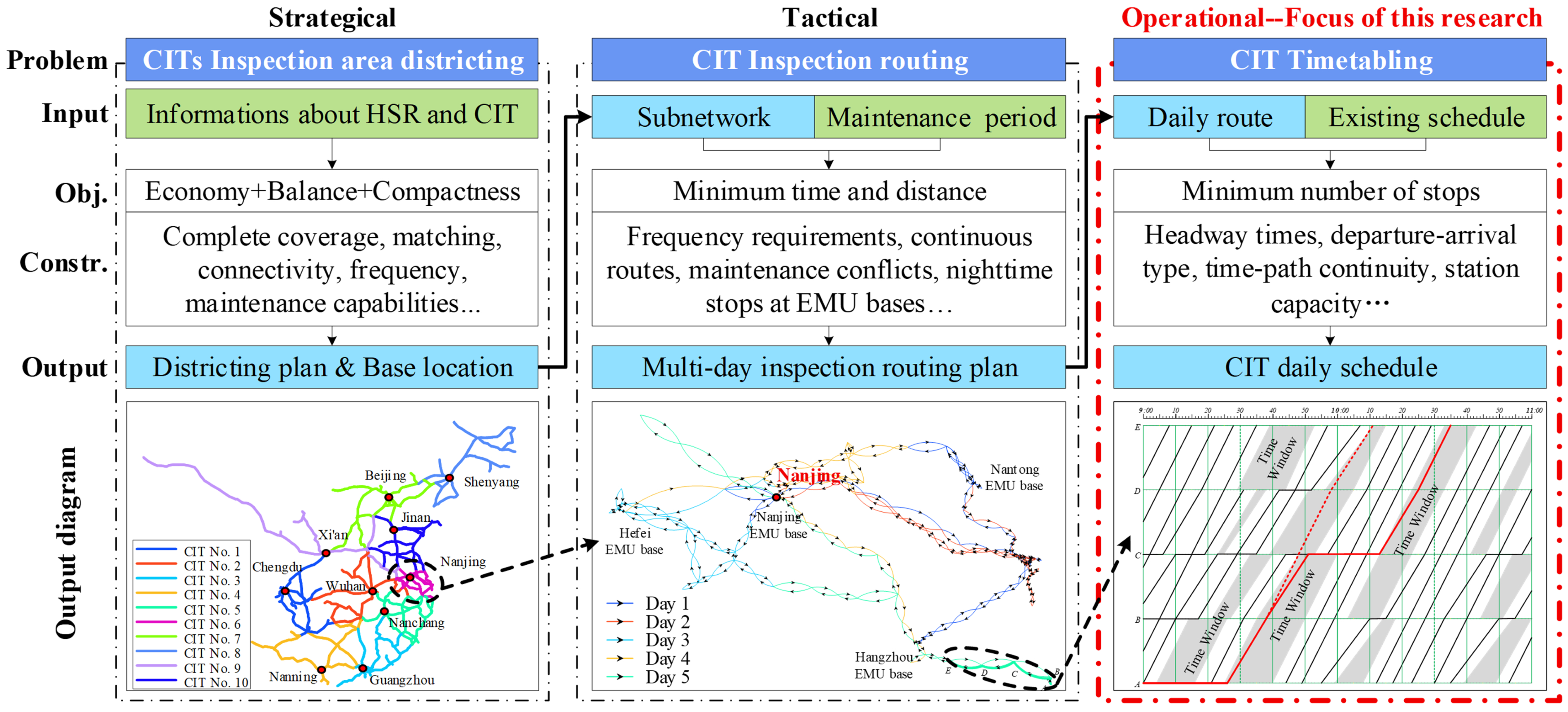
The planning of CIT operations can be conceptually divided into three hierarchical decision-making levels to reduce modeling complexity [2], as shown in Figure 1. (1) Strategic Level: Based on the heterogeneity between CIT attributes and HSR section characteristics, inspection regions are allocated to each CIT to simplify the multi-train collaboration problem into a single-train routing problem. (2) Tactical Level: Within each inspection region, the inspection paths and overnight electric multiple unit (EMU) bases for CIT are determined, considering factors such as required inspection frequencies, technical compatibility, and nighttime maintenance windows. (3) Operational Level: Given the inspection path for each day, detailed arrival and departure times at each station must be arranged such that CIT can be inserted into existing timetables without disrupting passenger train operations. The goal is to minimize unnecessary stops and ensure as many track segments as possible are inspected at the target operating speed.

This study focuses on the operational-level planning problem, where one of the most critical challenges lies in integrating CIT into pre-established, passenger-centric train schedules. In practice, CIT timetable planning is usually a highly experience-dependent and iterative task. Timetable planners must manually search for feasible time intervals in a dense passenger timetable, check headway requirements section by section, avoid conflicts with station capacity-saturated periods, and ensure that the CIT can complete the inspection path within the prescribed daily time range. This process becomes particularly difficult when the inspection path contains multiple intermediate stations, turnaround operations, and discrete feasible time windows. A local decision, such as adding one intermediate stop or delaying the CIT by several minutes at one station, may change the departure-arrival type of the following sections and further trigger new conflicts in downstream sections. Therefore, manual scheduling requires repeated trial-and-error adjustments and extensive conflict checking, which is time-consuming and may fail to fully exploit the residual capacity of the existing timetable. These practical challenges demonstrate the need for a systematic modeling approach that can explicitly describe feasible operating regions and efficiently generate a conflict-free CIT timetable.

The high density of scheduled passenger services, combined with the rigidity imposed by advance ticket sales, substantially restricts the feasible solution space for integrating CIT operations. Any viable inspection timetable must be developed without altering the trajectories or timings of existing passenger trains, thereby necessitating strict adherence to multiple operational constraints, including headway separations, directional track usage conflicts, and station capacity limits [3]. Under such tightly constrained temporal and spatial conditions, generating conflict-free and operationally feasible CIT timetables, while simultaneously ensuring the integrity of regular passenger train services, presents a highly complex and time-critical optimization problem.

Although the Additional Train Scheduling Problem (ATSP) is a common practice in railway timetable planning and adjustment, there is still no universally standardized definition of this term in the railway literature [4,5,6,7,8]. In this study, ATSP refers to the problem of scheduling one or more additional trains within an existing timetable to satisfy new operational demands while maintaining the feasibility of the overall train schedule. It is a complex programming problem at the network level that requires consideration of many factors, such as network constraints for railroads, the tracking headway time, conflicts in station capacity, passenger demand, turnover of Electric Multiple Units (EMUs), etc.

Research on the ATSP can be broadly categorized into two types: (1). problems that allow adjustments of other train lines [6,7,8]; (2). problems under the condition of an unchanged existing schedule [5,9,10,11,12]. The first category of problems mainly arises at the preparation stage of the operation plan: When scheduling additional trains, if all trains have not sold tickets in advance, the timetable of other trains can be adjusted. The latter application scenario is mainly for temporary additional trains operated on holidays and high-speed express trains, both of which have the common characteristic of being scheduled on short notice. At this time, the timetable of other trains has already been announced, and the tickets have been sold in advance; therefore, the timetable of the original train cannot be changed in principle. In this research, adding CIT’s train line is carried out under the condition of passenger train priority, which belongs to the new application scenario of the second category; this is essentially the problem of temporal and spatial resource conflict deconfliction under the condition of time windows.

1.2. Contribution

Efficient integration of CIT services can improve infrastructure inspection efficiency without requiring additional railway capacity resources, thereby contributing to the sustainable operation of high-speed railway systems. The main contributions of this study are summarized as follows:

• A Mixed-Integer Linear Programming (MILP) model is developed to address the problem of inserting a CIT into an existing high-density passenger timetable. The model explicitly captures the CIT’s arrival and departure times at intermediate stations, as well as its operational departure–arrival type, as decision variables. A novel linear formulation of time-window-based headway constraints is proposed, which offers improved tractability over traditional train-to-train headway constraints, especially under high traffic density conditions. The objective is to minimize the number of CIT stops—subject to station capacity and without disrupting scheduled passenger trains—in order to maximize inspection coverage at the highest possible operational speed. This enables more efficient diagnostics of potential infrastructure defects along the inspected route.
• To further enhance computational efficiency and scalability, this paper introduces a feasible region-based discrete space–time network modeling approach, which abstracts residual capacity within the timetable into a feasible event arc network (FEAN). Different from conventional space–time network methods that first generate a large number of candidate arcs and then identify conflicts through additional constraints, the proposed FEAN approach embeds feasibility screening directly into the network construction process. Specifically, event arcs are generated only when they satisfy the corresponding departure/pass and arrival/pass time windows, which makes the arc generation process explicitly time-window-driven. Moreover, the acceleration and deceleration effects associated with different departure–arrival types are incorporated into the travel time of event arcs rather than being simplified as fixed minimum or maximum running times. In addition, station capacity-saturated periods are handled during network construction by deleting the corresponding dwell arcs, so station capacity constraints are reflected structurally in the generated network. Consequently, the original scheduling problem is equivalently transformed into a classical shortest path problem on a customized feasible subnetwork, significantly reducing the computational burden while retaining modeling fidelity.

The remainder of this paper is organized as follows. Section 2 reviews the relevant literature on train scheduling and the ATSP. Section 3 presents the traditional mixed-integer programming formulation for the CIT timetable insertion problem. Section 4 develops the proposed feasible region-based space–time network modeling approach and reformulates the original problem as a shortest path problem. Section 5 reports the computational experiments and analyzes the effectiveness and efficiency of the proposed method. Finally, Section 6 concludes this paper and outlines directions for future research.

2. Literature Review

Compared with classical train timetabling and rescheduling problems, ATSP has received relatively less attention [4,7,8]. It dates back to the research of Ingolotti [10], Burdett [4], and Cacchiani [5], who focused on ATSP for freight trains. In recent years, the growing and time-varying passenger travel demand for high-speed railway has brought new requirements for the formulation of schedules and timely adjustment, which has focused increasing attention on the problem of adding additional lines [6,7,8,13].

Table 1. Literature review on ATSP.

Modelling Approaches	Author	Passenger /Freight	Other Trains Can Be Adjusted	Optimization Objectives	Single/Double-Track (1/2 Way)	Additional Time for Start/Stop	Station Capacity	Model Features	Solving Methods
Event–Activity Network	Ljunggren [12]	Freight	×	Improve robustness	Mix (2)	/	/	Nonlinear	Computer simulation
	Tan [8]	Passenger	√	1. Min time spent 2. Min adjustment	Double (1)	√	/	MIP	Genetic algorithm
	Flier [9]	Passenger	×	Improve robustness	Single (2)	/	/	Nonlinear	Shortest paths in conflict graphs
Alternative Graph	Burdett [4]	Freight	√ & ×	Finding viable solutions	Single (2)	/	/	Nonlinear	SA
	Tan [14]	Passenger	√	Min adjustment	Double (1)	√	√	ILP	Branch delimitation + local search
Space–Time Network	Cacchiani [5]	Freight	×	Min time spent	Mix (2)	/	/	ILP	HA based on Lagrangian
	Jiang [7]	Passenger	√	1. Max No. of adding trains 2. Min adjustment	Double (2)	√	√	ILP	HA based on Lagrangian
	Liu [11]	Passenger	×	1. Min operating costs 2. Max passenger satisfaction	Double (1)	/	/	MIP	CPLEX
	Gao [13]	Passenger	√	Min time spent	Double (1)	/	/	ILP	HA based on Lagrangian
	Jiang [15]	Passenger	√	1. Max No. of adding trains 2. Min adjustment	Double (2)	/	/	ILP	HA based on Lagrangian
Modelling Directly	Gao [6]	Passenger	√	1. Min time spent 2. Min adjustment	Double (2)	√	√	MIP	Gurobi + three-stage processing
	Ingolotti [10]	Freight	×	Min time spent	Single (2)	/	√	ILP	HA with sequential decision-making
	Liu [16]	Passenger	×	1. Min operating costs 2. Min time spent 3. Max passenger satisfaction	Double (1)	/	/	MIP	CPLEX

Remarks: ILP—integer linear programming model; MIP—mixed integer linear programming model; HA—heuristic algorithms; SA—simulated annealing algorithm.

provides a comprehensive overview of the studies on ATSP in the past 20 years, and it categorizes and summarizes them according to different modelling approaches.

2.1. Modelling Approach Based on Event–Activity Network

Event–activity networks are a widely used method for scheduling problems with time constraints [17,18,19]. This approach abstracts events as nodes and represents conflicts between activities and events over time as edges, thus constructing an abstract graph that describes the scheduling problem [20,21]. Tan [8] aimed to minimize the adjustment of existing trains and the running time of new trains, considering constraints such as train tracking intervals, stop duration ranges, and departure and arrival times. She developed a mixed-integer programming model based on the event–activity graph and designed an improved genetic algorithm, adding 10 new trains to a schedule of 186 trains. Ljunggren [12] and Flier [9] focused on the robustness of new train operation plans, but their models were nonlinear, leading them to use computer simulations and shortest path methods in conflict identification graphs for their solution approaches.

2.2. Modelling Approach Based on Alternative Graph

D’Ariano et al. [22,23] proposed the use of alternative graphs to study conflict resolution in railway transport organization, naming it “Railway Traffic Optimization by means of Alternative Graph” (ROMA). Since then, ROMA has become a commonly used tool in train timetable research [24,25,26]. The problem of adding tracks is a branch of timetable problems; thus, the relevant research methods also apply to the ATSP. Burdett [4], based on the method of alternative graphs, abstracted the ATSP in train operation diagrams as a hybrid job shop scheduling problem with time window constraints, defining the earliest and latest times for the start and end of train operation and stop events and constructing a corresponding analytical model. In terms of the solution algorithm, a constructive algorithm was first used to schedule new trains, followed by a conflict resolution repair program based on simulated annealing. The author also discussed two scenarios, fixed and non-fixed train timetables, with the maximum scale of the designed case being 11 stations, 54 existing trains, and five additional trains. Building on this, Tan [14] conducted more refined and detailed modeling down to each track, switch, and block section, aiming to minimize the adjustment of existing trains. They designed a phased iterative solution algorithm that combines branch-and-bound with local search, achieving the goal of adding 1 to 15 train lines to the timetable of eight stations with 36 existing trains.

2.3. Modelling Approach Based on Space–Time Network

The method based on space–time networks is also widely used in timetable problems, with principles closely aligned with the definition of train operation diagrams [27]. This method constructs stations as discrete nodes at a certain precision to represent the arrival and departure of trains; arcs connecting adjacent station nodes represent train operations in the intervals, and arcs between nodes of the same station represent the stopping process of trains [28,29]. Cacchiani [5] was the first to apply this method to ATSP while researching freight train operation planning. Given that the context involves a mixed single and double track network, he considered not only the tracking intervals for arrivals and departures at stations but also the passing intervals and different arrival intervals. However, due to a lack of constraints, arcs connecting arbitrary departure and arrival nodes between interval terminal stations were included in the model, resulting in a vast scale of conflict constraints between trains. Building on this, Jiang [7,15] explored a scenario where the existing train timetable and stopping schedules are adjustable, aiming to maximize the number of new trains and minimize the adjustments of existing trains. He constructed an integer linear programming model and designed a Lagrangian-based heuristic algorithm, also incorporating additional time segments for stops in the dynamic programming process. Furthermore, Liu [16] and Gao [13] employed similar methods to study the ATSP in high-speed rail operation diagrams under the constraints of non-adjustable and adjustable existing train timetables, respectively, but neither considered additional stop time segments or station capacity constraints.

2.4. Non-Graphical Modeling Approach

In addition to methods based on graphical analysis, some researchers construct models directly according to train operation organization rules. This type of method is also known as the big-$M$ formulation [30]. It typically represents the arrival and departure times of trains as discrete or continuous decision variables and additionally introduces binary sequence variables to handle potential headway conflict relationships between trains [31]. Ingolotti et al. [10] proposed an integer linear model to minimize the traversal time of newly added freight trains under fixed passenger schedules, incorporating constraints such as station capacity and single-track conflicts. To improve efficiency, they designed a sequential heuristic using reference-station-based priority rules. Building on this, Gao et al. [6] developed a bi-objective mixed-integer model for high-speed rail operations, balancing new train runtime and disruption to existing services. Their model accounted for track conflicts, stop decisions, and acceleration constraints, and they employed a three-stage solution method with Gurobi. Liu and Cao [11] further incorporated passenger demand, formulating a multi-objective model to minimize operational cost, travel time, and unmet demand. Their approach jointly optimized train count, operational zones, and stop patterns and was solved using CPLEX.

Recent studies have further shown that railway operation optimization is moving toward integrated planning and intelligent decision-support frameworks. For example, integrated optimization has been applied to coordinate train scheduling with rolling stock circulation planning [32] and to jointly optimize line planning and additional train scheduling under fluctuating passenger demand [33,34]. Station-level operational decision support has also been strengthened through real-time train rescheduling and replatforming models, which can generate high-quality dispatching plans for complex passenger stations within short computation times [35]. In addition, the coordination between transportation and maintenance has received increasing attention, with recent studies integrating train timetabling, maintenance window setting, and maintenance activity scheduling to balance train operation efficiency and infrastructure maintenance requirements [36,37]. Alongside these railway-specific studies, recent transportation optimization research has also emphasized data-driven forecasting, intelligent decision support, and hybrid optimization strategies for complex and dynamic operational scenarios [38,39]. These developments indicate that railway and transportation operation optimization is increasingly characterized by integrated modeling, data-driven decision support, and rapid solution techniques. However, most existing studies focus on passenger or freight service planning, rolling stock circulation, station rescheduling, or maintenance-window coordination, while the operational insertion of CIT paths into a fixed high-density passenger timetable remains insufficiently explored.

2.5. Gaps Analysis

Existing research on the ATSP provides valuable references for the formulation of CIT inspection plans. However, due to the specific backgrounds applicable to various methods, these cannot be directly applied to address the scheduling for CIT. The following summarizes the differences and limitations of existing ATSP research compared to CIT planning:

(1) Inconsistent Consideration of Whether Existing Train Timetables Are Adjustable: In passenger train ATSP, existing train schedules are generally adjustable, typically aiming to minimize the amount of adjustment. In contrast, in freight train ATSP, existing train schedules are generally non-adjustable, mainly due to the lower priority of freight trains compared to passenger trains. Considering the high proportion of cross-line trains in China’s high-speed rail operation, long pre-sale ticket cycles, and changes in CIT inspection demands, the planning of CIT inspection operations is more suitable in the background of fixed passenger train timetables.

(2) The Additional Time for Train Stops Must Be Considered: Given the high speed of trains, neglecting or simplifying the time taken for acceleration and deceleration will lead to discrepancies in actual planning. Few existing studies account for the additional time for train stops, but related methods require the introduction of stop decision variables and depend on large-scale constraints for identifying conflicts between trains, or they require algorithmic improvements for implementation. For CIT, consideration of additional stop time is essential, necessitating simpler modeling approaches and solution methods to enhance rapid decision-making capabilities.

(3) Although alternative graph-based modeling is effective for micro-level operational conflict identification, it is less suitable for large-scale network-level ATSP due to its limited capacity to handle many stations. Event–activity graphs and discrete space–time network methods, while intuitive and conceptually simple, rely heavily on large-scale conflict arc identification, which becomes computationally challenging as the network size increases. The process of manually constructing conflict sets in these models is particularly complex and may introduce significant computational overhead. Similarly, direct modeling approaches, while capable of handling specific operational constraints, also encounter challenges related to complex constraints and large-scale network requirements. These methods need further refinement and adaptation to effectively address the needs of network-level integration for CIT inspection routes and train scheduling.

3. Traditional Modeling

3.1. Assumptions

To enhance the operability of model formulation and solution, the following assumptions are adopted in this study:

(1) The arrival and departure times, as well as the operating sequence of passenger trains at intermediate stations in the existing timetable, are considered fixed and non-adjustable. This assumption reflects practical constraints in the Chinese HSR system, where passenger tickets are typically sold up to two weeks in advance. Modifying scheduled timetables would cause significant inconvenience to passengers. Furthermore, a large number of passenger trains operate across multiple lines, meaning that even minor adjustments could lead to widespread disruptions. This assumption has been thoroughly discussed in the motivation section of this paper.

(2) Only the inter-station operation plan of the CIT is considered in this model. The entry and exit operations related to the EMU base are not modelled explicitly, as these activities are generally handled by train dispatchers and station personnel based on operational needs and real-time conditions.

(3) The time windows representing conflicts in station capacity are assumed to be pre-processed and provided as input. These time windows are derived in advance based on the track occupancy plan and station interlocking scheme, thereby simplifying the modeling of station capacity constraints. In practical railway operations, such capacity-saturated periods can be obtained from the existing train timetable, station track-use plan, and interlocking route arrangement. Specifically, for each station, the occupation intervals of scheduled passenger trains on candidate receiving/departure tracks and related approach/departure routes are first identified. These intervals are then expanded according to the required route setting, release, and safety separation times. If all track-route combinations available for CIT reception or departure are occupied or blocked during a certain period, this period is recorded as a station capacity-saturated period and used as an input to the proposed model.

3.2. Symbol Definition

The definitions of the symbols used in the model and their value ranges are described in

Table 2. Symbol definition.

Type	Symbol	Description	Range
Set	$E$	$E=\left\{\left(i_r,j_r\right)|1\le r\le \left|E\right|\right\}$, the set of sections in inspection path.	/
	${TWQ}_r$	${TWQ}_r=\left\{\left[{TWQ}_r^{S,ti},{TWQ}_r^{E,ti}\right]\left|\right|ti\in {\mathbb{N}}^{+}\right\}$, the set of time ranges corresponding to the departure/pass time window of the r-th section.	/
	${TWD}_r$	${TWD}_r=\left\{\left[{TWD}_r^{S,ti},{TWD}_r^{E,ti}\right]\left|\right|ti\in {\mathbb{N}}^{+}\right\}$, the set of time ranges corresponding to the arrival/pass time window of the r-th section.	/
	${BH}_r$	${BH}_r=\left\{\left[{BH}_r^{S,tj},{BH}_r^{E,tj}\right]\left|\right|tj\in {\mathbb{N}}^{+}\right\}$, the set of capacity-saturated periods at the origin station of the r-th section.	/
	$R$	The set of sections that require turnaround after the CIT finishes the inspection task.	/
Index	$m$	Indicate the departure–arrival type of CIT at the stations of the section. Pass–pass taken as 1; start–pass taken as 2; pass–stop taken as 3; start–stop taken as 4.	{1,2,3,4}
	$r$	Indicates section order.	${\mathbb{N}}^{+}$
	$ti$	Indicates time window order.	${\mathbb{N}}^{+}$
	$tj$	The order of the capacity saturation time window, with the special note that there are differences in $tj$ for different sections.	${\mathbb{N}}^{+}$
Parameter	${BT}_r$	Indicate the time spent when CIT passes through at both stations in section $r.$	${\mathbb{N}}^{+}$
	$t_m^{\mathrm{F}\mathrm{J}}$	The additional time spent corresponding to the departure–arrival type $m$. When $m$ is taken to be 1–4, this parameter is, respectively, taken to be 0, 2, 3, and 5.	{0,2,3,5}
	$t^{\mathrm{S}\mathrm{T}}$	Earliest check-in time; if 8:00, then take the value 480.	${\mathbb{N}}^{+}$
	$t^{\mathrm{T}\mathrm{C}\mathrm{D}}$	Last check-out time; if 20:00, then takes the value 1200.	${\mathbb{N}}^{+}$
	$t^{\mathrm{T}\mathrm{B}}$	Minimum time for turnaround, usually taken as 15 min.	${\mathbb{N}}^{+}$
Variable	${MO}_r^m$	Decision variable, which indicates inspection of the $r$th section with type $m$.	{0,1}
	$T_r^{\mathrm{L}}$	Decision variable, which indicates the departure time of the CIT leaving the first station of section $r$.	${\mathbb{N}}^{+}$
	$T_r^{\mathrm{W}}$	Auxiliary decision variable, which indicates the waiting time of the CIT at the first station of section $r$.	$\mathbb{N}$
	$T_r^{\mathrm{A}}$	Auxiliary decision variable, which indicates the arrival time of the CIT at the end station of section $r$.	${\mathbb{N}}^{+}$
	${TQ}_r^{\mathrm{S},ti}$	Auxiliary decision variable, which indicates whether the $ti$th lower bound of departure/pass time window is less than or equal to $T_r^{\mathrm{L}}$, if it is taken as 1; otherwise, it is taken as 0.	{0,1}
	${TQ}_r^{\mathrm{E},ti}$	Auxiliary decision variable, which indicates whether the $ti$th upper bound of departure/pass time window is less than or equal to $T_r^{\mathrm{L}}$, if it is taken as 1; otherwise, it is taken as 0.	{0,1}
	${TD}_r^{\mathrm{S},ti}$	Auxiliary decision variable, which indicates whether the $ti$th lower bound of arrival/pass time window is less than or equal to $T_r^{\mathrm{A}}$ if it is taken as 1; otherwise, it is taken as 0.	{0,1}
	${TD}_r^{\mathrm{E},ti}$	Auxiliary decision variable, which indicates whether the $ti$th upper bound of arrival/pass time window is less than or equal to $T_r^{\mathrm{A}}$ if it is taken as 1; otherwise, it is taken as 0.	{0,1}

below.

3.3. Objective Function

Operators expect the CIT to inspect each section at the maximum speed permitted by the line, because full-speed inspection is more beneficial for detecting potential infrastructure defects. The reason is that frequent stops interrupt the continuous running state of the CIT and introduce repeated deceleration, stopping, and re-acceleration processes. These processes reduce the proportion of sections inspected at the target operating speed and may affect the continuity and stability of inspection data. Therefore, the formulation of the CIT timetable aims to improve the technical speed of CIT operations. From the perspective of inspection effectiveness, a higher proportion of full-speed inspection sections is beneficial for obtaining continuous and stable dynamic detection data, which supports more reliable infrastructure condition diagnosis. Some defects or performance abnormalities can be accurately identified only under target-speed operating conditions, such as pantograph–catenary interaction abnormalities, communication latency, and other dynamic system responses. In this study, the inspection path and total inspection mileage are given in advance; therefore, the main factor affecting the technical speed is not the route length but the additional running time caused by deceleration, stopping, and acceleration at intermediate stations.

Directly maximizing technical speed would introduce a fractional objective involving total inspection mileage and total running time, which would increase the complexity of the model. Moreover, in practical CIT operations, reducing intermediate stops directly increases the number of sections that can be inspected at the target operating speed. Thus, stop reduction contributes not only to higher operational efficiency but also to improved inspection data continuity, stability, and diagnostic reliability. Therefore, minimizing the number of stops is adopted as a linear and operationally interpretable surrogate objective for improving technical speed. Accordingly, the objective function is formulated to minimize the total number of sections operated under the start–stop and pass–stop types.

$$\min Z=\sum _{r=1}^{\left|E\right|}\sum _{m=3}^4{MO}_r^m.$$

(1)

3.4. Constraints

There are numerous constraints to consider when scheduling for CIT, including the following 13 categories:

(1) Departure–Arrival Type Unique Constraints: Each section can be detected only once with a unique departure–arrival type.

$$\sum _{m=1}^4{MO}_r^m=1 1\le r\le \left|E\right|.$$

(2)

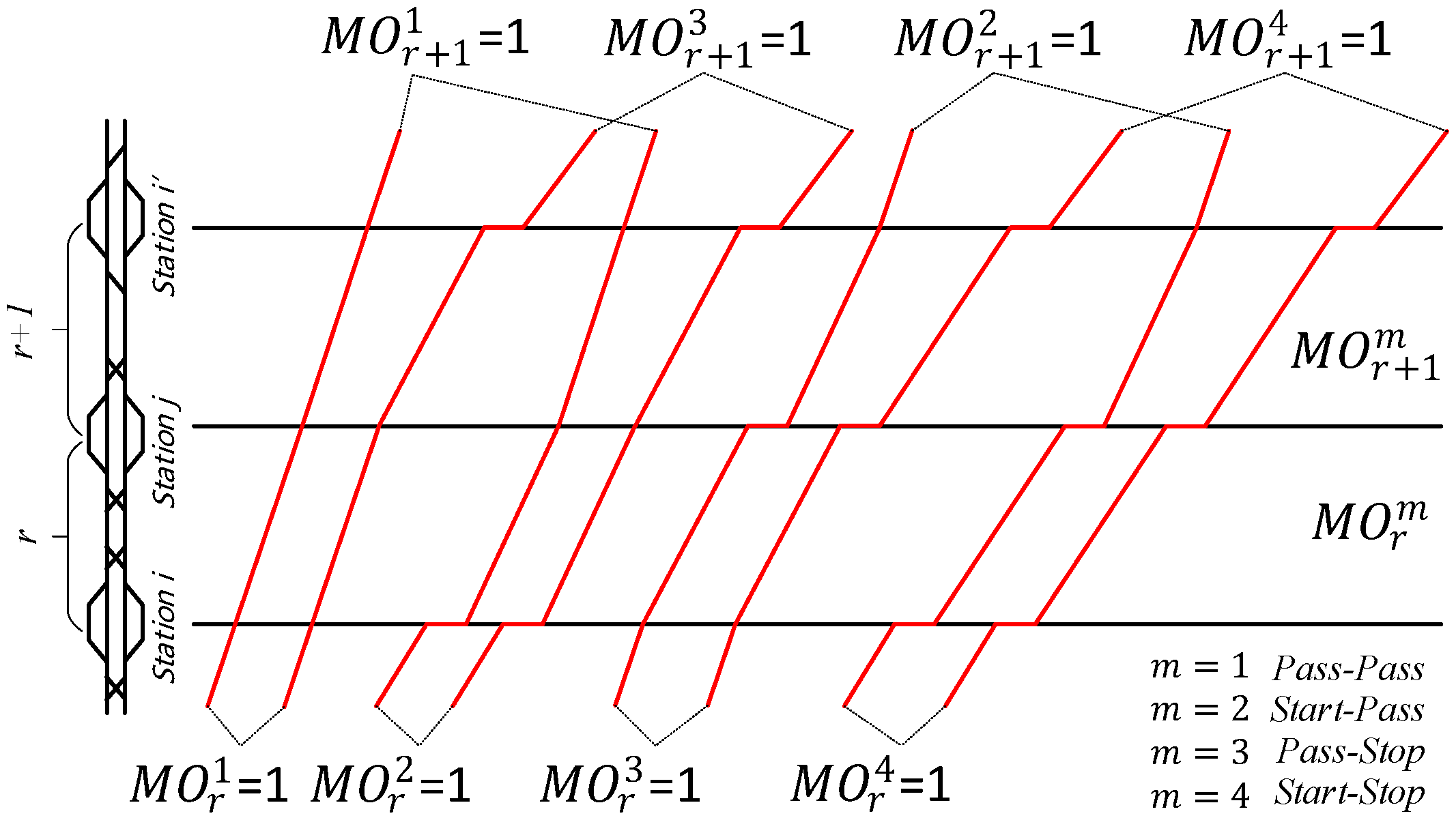
(2) Departure–Arrival Type Association Constraints: The departure–arrival type applied in each section is closely related to the type of the previous section. As shown in Figure 2, taking station j as an example, after the CIT completes the inspection task of the rth section, the type that can be chosen is either passing or stopping, while it further determines the type that can be chosen for the r + 1th section.

$${MO}_r^1+{MO}_r^2={MO}_{r+1}^1+{MO}_{r+1}^3 1\le r\le \left|E\right|-1.$$

(3)

$${MO}_r^3+{MO}_r^4={MO}_{r+1}^2+{MO}_{r+1}^4 1\le r\le \left|E\right|-1.$$

(4)

(3) Departure–Arrival Type Constraints for Check-In/Out: Since the check-in/out of the inspection team needs to be performed at the station, the first section can only choose the start–stop or start–pass mode; the last section can only choose the start–stop or pass–stop mode.

$${MO}_1^2+{MO}_1^4=1.$$

(5)

$${MO}_{\left|E\right|}^3+{MO}_{\left|E\right|}^4=1.$$

(6)

(4) Departure–Arrival Type Constraints at Turnaround Stations: Turnarounds at stations require the driver to transfer the direction of the CIT’s operation. In this case, the departure–arrival type of the previous section can only be pass–stop or start–stop, and the next section can only be start–stop or start–pass.

$${MO}_r^3+{MO}_r^4=1 \forall r\in R.$$

(7)

$${MO}_{r+1}^2+{MO}_{r+1}^4=1 \forall r\in R.$$

(8)

(5) Constraints Between Schedule and Departure–Arrival Type: CIT must follow the basic rules of train operation, and the inspection time cost of each section is not only related to the pure operation time but also related to the departure–arrival type of the train at the first and last station of the section. The different modes correspond to different additional time spent, where the check-in station is initialized to $T_1^{\mathrm{L}}=t^{\mathrm{S}\mathrm{T}}$.

$$T_r^{\mathrm{A}}=T_r^{\mathrm{L}}+{BT}_r+\sum _{m=1}^4\left(t_m^{\mathrm{F}\mathrm{J}}{MO}_r^m\right) 1\le r\le \left|E\right|.$$

(9)

(6) Recursive Constraints for Arrival and Departure Times: The arrival and departure times of CIT at each station are related to the dwell time.

$$T_{r+1}^{\mathrm{W}}=T_{r+1}^{\mathrm{L}}-T_r^{\mathrm{A}} 1\le r\le \left|E\right|-1.$$

(10)

$$T_r^{\mathrm{W}}\ge 0 1\le r\le \left|E\right|.$$

(11)

(7) Relationship Between Departure–Arrival Type and Waiting Time: The dwell time is closely related to the departure–arrival type of the previous section: when CIT passes through the station, the dwell time can only be taken as 0; only when CIT stops at the station can the dwell time be taken as a positive value.

$$M\left(\sum _{m=3}^4{MO}_r^m\right)\ge T_{r+1}^{\mathrm{W}} 1\le r\le \left|E\right|-1.$$

(12)

(8) Turnaround Time Constraint: When CIT turns around at a station, the waiting time shall not be less than the minimum time $t^{\mathrm{T}\mathrm{B}}$.

$$T_{r+1}^{\mathrm{W}}-t^{\mathrm{T}\mathrm{B}}\ge 0 \forall r\in R.$$

(13)

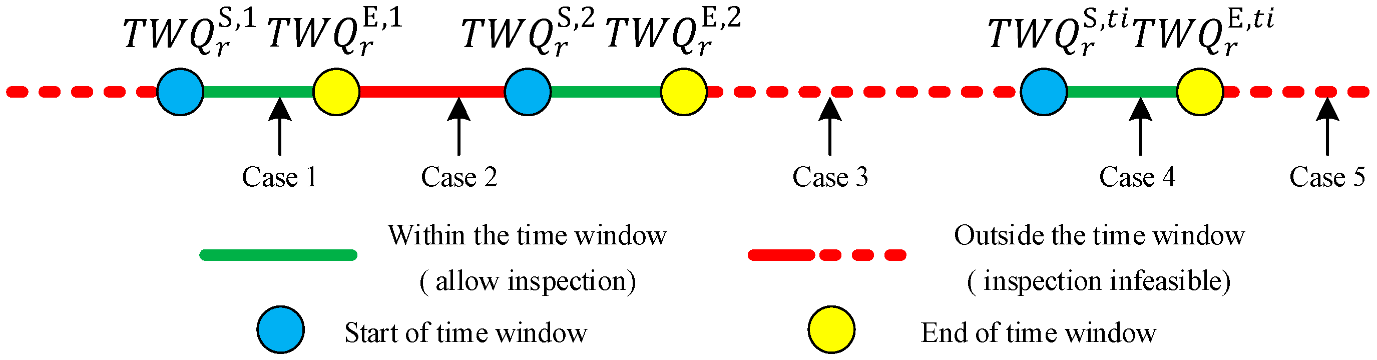
(9) Departure/Pass Time Window Constraints: To avoid operational conflicts between CIT and passenger EMUs, the time for CIT to leave the station and enter the section for inspection must meet the headway time requirement, meaning that the departure time must fall within the departure/pass time window. Unlike existing studies, which typically consider a single time window (Figure 3) with only one time range constraint, the CIT is influenced by passenger trains, resulting in large, discrete time windows for the section, with no unified patterns for description. This significantly increases the complexity of modeling.

Further analyses of the structural characteristics of time windows reveal that the left and right endpoints of the time windows always appear in pairs, as shown in Figure 3. When the departure time is outside the time window, the number of left endpoints and right endpoints to the left of the departure time is equal. When the departure time is within the time window, the number of left endpoints (including overlaps) to the left of the departure time is exactly one more than the number of right endpoints. Based on this analysis, the departure/pass time window constraint can essentially be transformed into a determination of the positions and quantities of the left and right endpoints of the time windows.

$${TWQ}_r^{\mathrm{S},ti}{TQ}_r^{\mathrm{S},ti}\le T_r^{\mathrm{L}} \forall ti, 1\le r\le \left|E\right|.$$

(14)

$${TWQ}_r^{\mathrm{S},ti}+{TQ}_r^{\mathrm{S},ti}M>T_r^{\mathrm{L}} \forall ti, 1\le r\le \left|E\right|.$$

(15)

$${TWQ}_r^{\mathrm{E},ti}{TQ}_r^{\mathrm{E},ti}<T_r^{\mathrm{L}} \forall ti, 1\le r\le \left|E\right|.$$

(16)

$${TWQ}_r^{\mathrm{E},ti}+{TQ}_r^{\mathrm{E},ti}M\ge T_r^{\mathrm{L}} \forall ti, 1\le r\le \left|E\right|.$$

(17)

$$\sum _{ti}{TQ}_r^{\mathrm{S},ti}-\sum _{ti}{TQ}_r^{\mathrm{E},ti}=1 1\le r\le \left|E\right|.$$

(18)

(10) Departure/Pass Time Window Constraints: Similarly to the departure/pass time window constraint, the main purpose of the arrival/pass time window constraint is to avoid operational conflicts between the CIT and passenger trains, which can be modelled with reference to the departure/pass time window constraint.

$${TWD}_r^{\mathrm{S},ti}{TD}_r^{\mathrm{S},ti}\le T_r^{\mathrm{A}} \forall ti, 1\le r\le \left|E\right|.$$

(19)

$${TWD}_r^{\mathrm{S},ti}+{TD}_r^{\mathrm{S},ti}M>T_r^{\mathrm{A}} \forall ti, 1\le r\le \left|E\right|.$$

(20)

$${TWD}_r^{\mathrm{E},ti}{TD}_r^{\mathrm{E},ti}<T_r^{\mathrm{A}} \forall ti, 1\le r\le \left|E\right|.$$

(21)

$${TWD}_r^{\mathrm{E},ti}+{TD}_r^{\mathrm{E},ti}M\ge T_r^{\mathrm{A}} \forall ti, 1\le r\le \left|E\right|.$$

(22)

$$\sum _{ti}{TD}_r^{\mathrm{S},ti}-\sum _{ti}{TD}_r^{\mathrm{E},ti}=1 1\le r\le \left|E\right|.$$

(23)

(11) Availability of Track to Receive CIT: When CIT chooses to stop at the station, the dwell period cannot intersect with the capacity-saturation period.

$$\left\{\begin{array}{cc}\mathrm{i}\mathrm{f}& T_r^{\mathrm{W}}>0\\ \mathrm{t}\mathrm{h}\mathrm{e}\mathrm{n}& \left[T_{r-1}^{\mathrm{A}},T_r^{\mathrm{L}}\right]\cap \left[{BH}_r^{\mathrm{S},tj},{BH}_r^{\mathrm{E},tj}\right]=\mathrm{\varnothing }\end{array}\right. \forall tj, 2\le r\le \left|E\right|.$$

(24)

(12) Termination Constraint: The inspection must be completed within the time limit of the check out.

$$T_{\left|E\right|}^{\mathrm{A}}\le t^{\mathrm{T}\mathrm{C}\mathrm{D}}.$$

(25)

(13) Other Constraints:

$${MO}_r^m{,TQ}_{\left(i,j\right),r}^{\mathrm{S},ti},{TQ}_{\left(i,j\right),r}^{\mathrm{E},ti},{TD}_{\left(i,j\right),r}^{\mathrm{S},ti},{TD}_{\left(i,j\right),r}^{\mathrm{E},ti}\in \left\{\mathrm{0,1}\right\}.$$

(26)

$$T_r^{\mathrm{L}},T_r^{\mathrm{A}},T_r^{\mathrm{W}}\in \mathbb{N}.$$

(27)

4. Feasible Region-Based Space–Time Network Modeling

The model formulated in Section 3 is a nonlinear mixed-integer programming model with high complexity, especially when the inspection path involves a large number of stations, and there are numerous time windows for each section. Directly solving the model under these conditions is extremely challenging. The main difficulty lies in the fact that the operational rules of CIT path scheduling, including headway requirements, departure/pass and arrival/pass time windows, acceleration/deceleration effects, station dwell decisions, turnaround constraints, and station capacity restrictions, are expressed as a large number of interrelated algebraic constraints in the traditional formulation.

In related studies on train scheduling and adjustment, some researchers have re-modelled the problem using methods such as event–activity network and space–time network. However, these methods often rely on establishing large-scale cluster constraints when dealing with different train arrival and departure intervals, leading to a dramatic increase in the number of constraints as the problem size grows [15]. Most modeling approaches based on space–time networks simplify the additional time by only using the maximum and minimum section times, neglecting the impact of the specific arrival and departure patterns at adjacent stations. The additional time refers to the extra running time incurred when a train stops at a station compared to the scenario where the train passes through without stopping. This deviation may result in the timetable being inexecutable in the actual transportation organization [13,15,28]. In addition, established space–time network modelling methods fail to consider conflict scenarios, such as station capacity saturation, and they do not incorporate relevant constraints into the network construction and subsequent modelling process.

To address the aforementioned challenges, this section draws on the analytical and modeling approaches of existing event–activity networks and space–time networks while also implementing necessary improvements. The essential idea of the proposed FEAN-based model is to transform the complex algebraic constraints in the traditional formulation into graph-based feasibility rules during network construction. In other words, the feasibility of CIT operations is no longer mainly guaranteed by adding large-scale constraints to the optimization model but by constructing a network that only retains feasible nodes and event arcs. A rapid decision-making theoretical framework will be constructed that is better suited for scheduling CIT, thereby addressing the limitations of current methods.

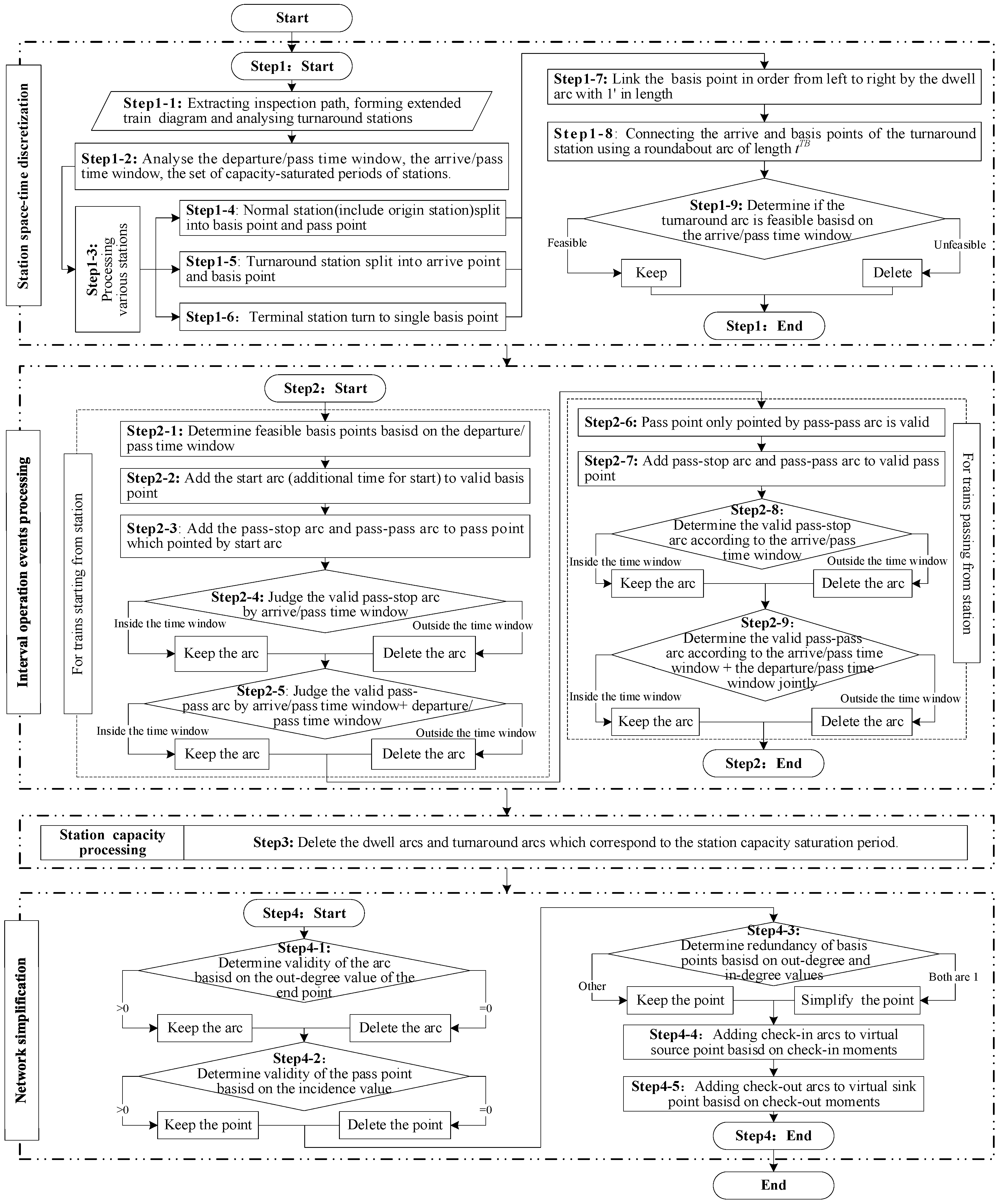
In the context of CIT operations, the schedules of passenger trains are non-adjustable, and time windows represent a critical characteristic of the problem. Therefore, the processing concepts from event–activity networks can be leveraged to utilize time-window information for determining the feasibility of various event arcs. Specifically, headway constraints are reflected by departure/pass and arrival/pass time-window screening, acceleration and deceleration effects are embedded in the travel times of different event arcs, and station capacity constraints are incorporated by deleting dwell arcs that overlap with capacity-saturated periods. The core principle of the improved space–time network modeling method is to identify all event arcs that satisfy the time-window conditions, thereby constructing a graphical representation of the feasible operating region for CIT path scheduling. On this basis, the original constrained scheduling problem is converted into a shortest path problem on the constructed FEAN, which strengthens the connection between the traditional mathematical formulation and the proposed graph-based model. This entire processing procedure encompasses four main components: station space–time discretization, interval operation events processing, station capacity processing, and network simplification (illustrated in Figure 4).

4.1. Station Space–Time Discretization

Firstly, analyze the CIT inspection task, including paths, turnaround stations, passenger train timetable, etc., and integrate them in section order to obtain an extended train operation diagram. Then, based on the headway time and station track allocation plan, the departure/pass time window, arrival/pass time window, and capacity-saturated periods for stations that are available for CIT are derived section by section.

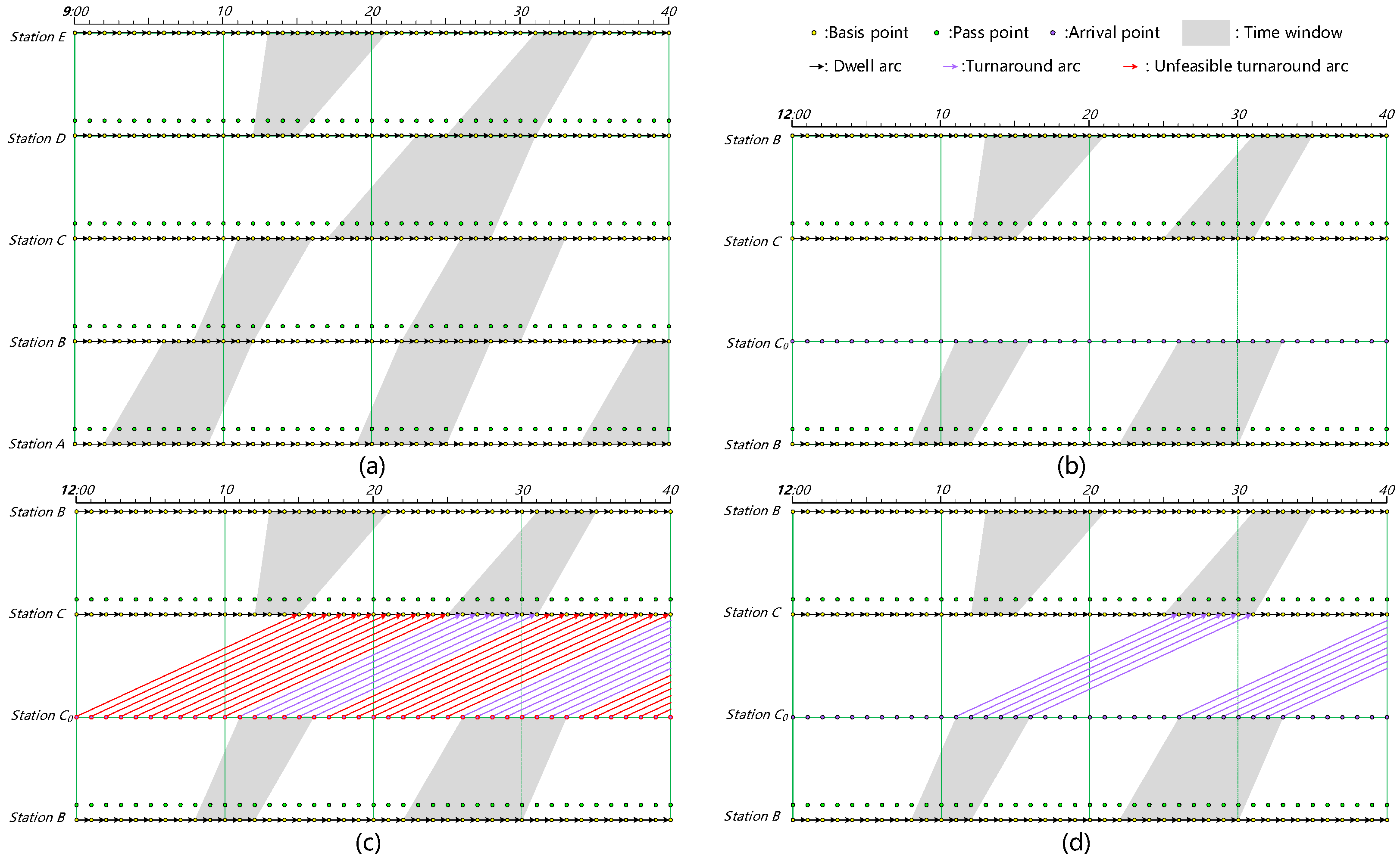
The next step will correspond to differentiated processing methods based on the different types of stations. For general stations, including daily check-in stations, such as stations A–D in Figure 5a, they are divided into basis points (yellow) and pass points (green) with an accuracy of 1 minute. When the inspection path involves a turnaround process, for the turnaround station C, it is necessary to refer to Figure 5b and place a virtual arrival point (purple C0) in front of station C. The original station is treated as a basis point (yellow) and a pass point (green) based on the general station. For the daily departure terminal station, as shown in station E in Figure 5a, it only needs to be discretized into basis points (yellow).

The basis points of each station are sequentially connected from left to right using dwell arcs (as shown in Figure 5a) to represent the stopping state of the train at the station. The number of dwell arcs occupied corresponds to the number of stopping minutes. For the turnaround operation station, based on the shortest required time for the operation, a turnaround arc is added between each virtual arrival point (purple C0) and the basis point, as shown in Figure 5c.

Further analysis shows that not all of the constructed turnaround arcs are feasible, which mainly depends on the arrival/pass time window of station C. As shown in Figure 5c, the start point of the red turnaround arc is not within the arrival/pass time window range of station C. Each virtual arrival point must be an isolated point with an in-degree of 0, so it can be deleted to reduce the network size. The final simplified result is shown in Figure 5d.

4.2. Interval Operation Events Processing

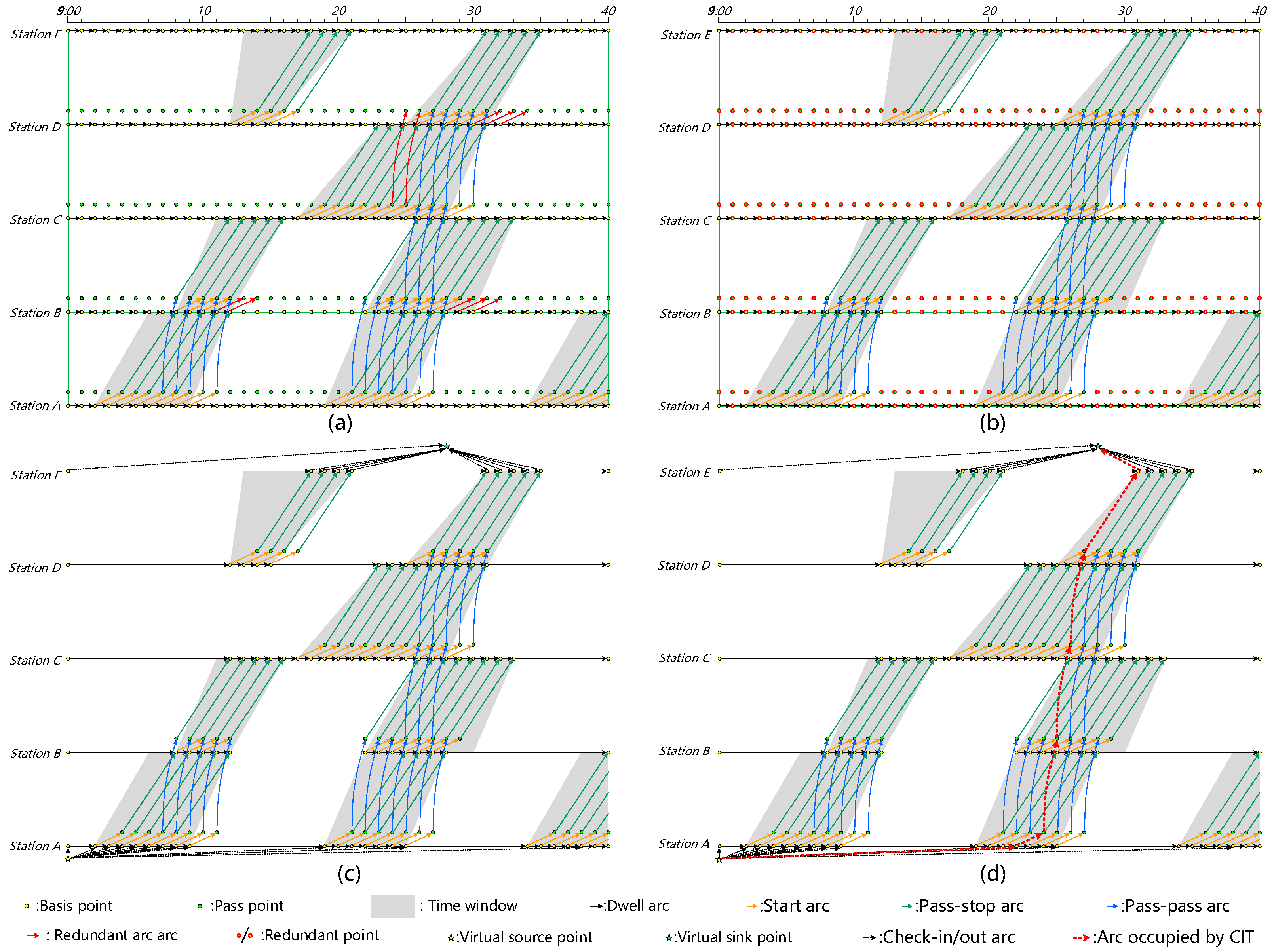
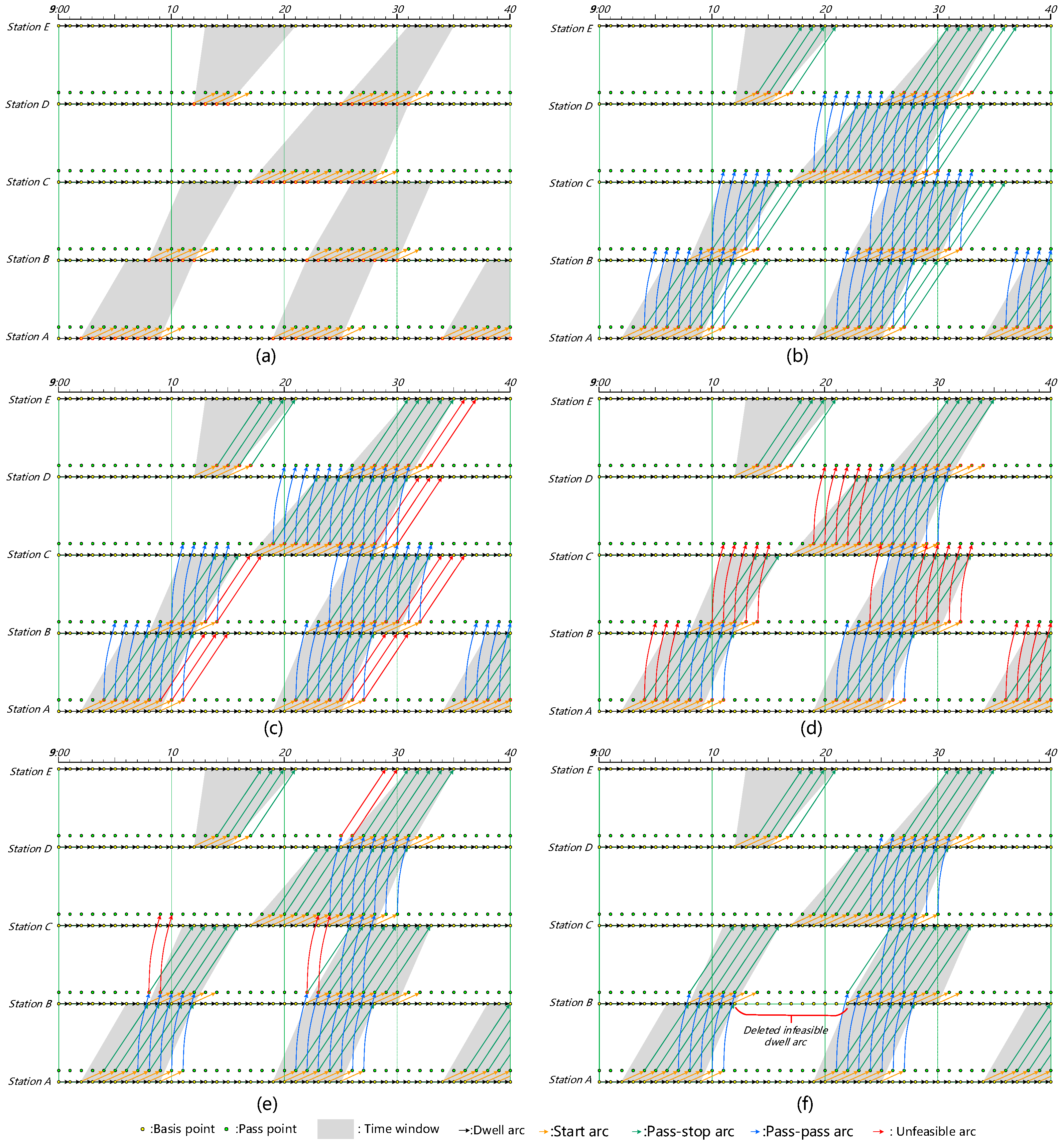
The expression of the operating status of trains in a section is the key to space–time network processing, and here, it is divided into trains starting from a station and trains passing from station to station. As shown in Figure 6a, each base point is determined to be a valid base point (yellow point on the red border) according to the departure/pass time window of the station, and then, the start arc (orange) is added to each valid base point according to the additional time of the starting time (2 min in the example). After completing the above steps, pass–stop arcs (green) and pass–pass arcs (blue) are added to the passing points activated by start arcs (green points on the red boundary) according to the basic time and the additional minutes of stopping, as shown in Figure 6b. The added arcs may not fulfill the time window restriction. Firstly, the infeasible pass–stop arcs are determined: If the end point of the pass–stop arc is outside the station arrival/pass time window, it is determined as an infeasible pass–stop arc (e.g., the red arc in Figure 6c); secondly, the infeasible pass–pass arcs are determined: The end point of the pass–stop arc is outside the station arrival/pass time window, and it is determined to be an infeasible pass–pass arc (e.g., the red arc in Figure 6)). Finally, the infeasible arcs are deleted.

The additional running time is used in the FEAN construction process to distinguish different departure–arrival types. Compared with a pass–pass operation, start–pass, pass–stop, and start–stop operations involve additional time losses caused by acceleration and/or deceleration. In this study, these additional time values are treated as empirical parameters and are set to 0, 2, 3, and 5 min for pass–pass, start–pass, pass–stop, and start–stop operations, respectively. These values are used to represent the relative time differences among different operating states. In practical applications, they can be recalibrated according to specific CIT operating performance, line speed conditions, train control requirements, and railway technical standards.

Although the above process involves some trains passing from station, there are still some pass–pass arc end points with out-degree 0 (e.g., the green point on the red boundary in Figure 6e), and these valid pass points can still be added with pass–stop arcs and pass–pass arcs. After the above addition steps, it is still necessary to refer to the arc feasibility determination rules to delete the infeasible event arcs to obtain a feasible event arc network, as shown in Figure 6f.

4.3. Station Capacity Processing

For station capacity constraints, the dwell arc of each station for the corresponding time period is deleted based on the station’s capacity-saturated time period, e.g., Station B [9: 12, 9: 22], as shown in Figure 6f.

4.4. Network Simplification

Further analysis indicates that there are still a large number of invalid arcs and isolated nodes in the feasible event arc network, so the network can be further simplified to improve the search speed. Firstly, the invalid arcs are determined and deleted according to the out-degree values of the arc endpoints, as shown in Figure 7a; the invalid passing points are determined and deleted according to the in-degree values, as shown in Figure 7b; the network is simplified for the large number of redundant basic points with out-degree and in-degree values of 1, as shown in Figure 7b. After the above steps, the streamlined feasible event arc network can be obtained. Finally, according to the check-in/out moments, the virtual source points, virtual sink points, check-in arcs (arc lengths are taken as 0), and check-out arcs (arc lengths are taken as 0) are added, as in Figure 7c.

Any reachable path from the source point to the sink point in Figure 7c corresponds to a feasible train line. It is easy to find the train line with the highest technical speed from station A to station E in the figure, as shown by the bolded red dashed arc in Figure 7d. Using the improved space–time network method in this paper and setting the length of all the dwell arcs to 0, the problem of adding additional train lines with the goal of obtaining the maximum technical speed of the CIT can be transformed into a classical shortest path problem. If the dwell arcs take the actual time length, the shortest path corresponds to the train line with the fastest average speed. Using the improved space–time network method, multiple optimal or similar paths can also be obtained, which can be further analysed for robustness, etc.

4.5. Model Reconstruction

Based on the FEAN, the original problem can be transformed into a classical shortest path problem, but it is still necessary to obtain a new model in order to easily solve the problem and improve the portability of the method.

i.

Symbol definition

The definitions of the symbols used in the new model and the range of values are described in

Table 3. Symbol definition.

Type	Symbol	Description	Range
Set	$G^{\mathrm{D}}$	The space–time network, $G^{\mathrm{D}}=\left(V^{\mathrm{D}},E^{\mathrm{D}}\right)$	/
	$E^{\mathrm{D}}$	Denote the set with event arcs, $E^{\mathrm{D}}=E^{{\mathrm{D}}_1}\cup E^{{\mathrm{D}}_2}\cup E^{{\mathrm{D}}_3}\cup E^{{\mathrm{D}}_4}\cup E^{{\mathrm{D}}_5}\cup E^{{\mathrm{D}}_6}$. $E^{{\mathrm{D}}_1}$ denotes the dwell arc; $E^{{\mathrm{D}}_2}$ denotes the turnaround arc; $E^{{\mathrm{D}}_3}$ denotes the start arc; $E^{{\mathrm{D}}_4}$ denotes the pass–stop arc; $E^{{\mathrm{D}}_5}$ denotes the pass–pass arc; $E^{{\mathrm{D}}_6}$ denotes the check-in/out arc.	/
	$V^{\mathrm{D}}$	Denote the set of points $V^{\mathrm{D}}=V^{\mathrm{B}}\cup V^{\mathrm{P}}\cup V^{\mathrm{A}}\cup v^{\mathrm{s}}\cup v^{\mathrm{m}}$. $V^{\mathrm{B}}$ denotes the set of basis points; $V^{\mathrm{P}}$ denotes the set of pass points; $V^{\mathrm{A}}$ denotes the set of arrival points; $v^{\mathrm{s}}$ denotes the virtual source point; $v^{\mathrm{m}}$ denotes the virtual sink point.	/
Index	$i,j$	Index of points, $i,j\in V^D$. Note that when taken as 1, it corresponds to the virtual source point $v^{\mathrm{s}}$; when taken as $\left|V^{\mathrm{D}}\right|$, it corresponds to the virtual sink point $v^{\mathrm{m}}$	/
	$\left(i,j\right)$	Index of event arcs, $\left(i,j\right)\in E^{\mathrm{D}},i\ne j$.	/
Parameter	$L_{\left(i,j\right)}$	Denote the time spent on the event arcs. When $\left(i,j\right)$ does not exist, it is taken as $+\infty$.	$\mathbb{N}$
	${\lambda }^k$	Corresponds to the weights of the different types of event arcs, $k\in \left\{\mathrm{1,2},\mathrm{3,4},\mathrm{5,6}\right\}$.	$\mathbb{R}$
Variable	$s_{ij}$	Decision variable corresponding to whether the event arc $\left(i,j\right)$ is used by CIT: taking 1 means use, and taking 0 means vice versa.	{0,1}

below.

iii.

Modelling

Based on the classical shortest path model, the objective function is improved so that the new model can express different optimization requirements. The model is shown in Equation (28), where the objective function is represented as the weighted sum of the costs of different types of event arcs, and the constraints mainly limit the continuity of the CIT from the virtual source to the virtual sink and the range of values of the decision variable $s_{ij}$.

$$\left.\begin{array}{c}\min Z={\displaystyle \sum _{k=1}^5}\left({\lambda }^k{\displaystyle \sum _{\left(i,j\right)\in E^{D_k}}}\left(L_{\left(i,j\right)}{s}_{ij}\right)\right),\\ \begin{array}{cc}s.t.& \left\{\begin{array}{c}{\displaystyle \sum _{\begin{array}{c}j=1\\ \left(i,j\right)\in E^{\mathrm{D}}\end{array}}^{\left|V^{\mathrm{D}}\right|}}{s}_{ij}-{\displaystyle \sum _{\begin{array}{c}j=1\\ \left(i,j\right)\in E^{\mathrm{D}}\end{array}}^{\left|V^{\mathrm{D}}\right|}}{s}_{ji}=\left\{\begin{array}{cc}1& i=1,\\ -1& i=\left|V^{\mathrm{D}}\right|,\\ 0& i\ne 1,\left|V^{\mathrm{D}}\right|,\end{array}\right.\\ s_{ji}\in \left\{\mathrm{0,1}\right\},\end{array}\right.\end{array}\end{array}\right\}.$$

(28)

When the arc weights (${\lambda }^1-{\lambda }^5$) are all taken as 1, the objective function accounts for the time costs of all types of event arcs. In this case, the shortest path corresponds to the train path with the minimum total travel time, namely the path with the fastest overall average speed. If ${\lambda }^1$ and ${\lambda }^2$ are set to 0 while ${\lambda }^3, {\lambda }^4, \mathrm{a}\mathrm{n}\mathrm{d} {\lambda }^5$ are set to 1, the dwell- and waiting-related costs are excluded from the objective function, and the model focuses on minimizing the number of operation-state changes associated with intermediate stops. This setting corresponds to improving the average speed after deducting stopping and waiting times, and it is consistent with the objective of reducing the number of CIT stops. Conversely, if ${\lambda }^1$ and ${\lambda }^2$ are set to 1 while ${\lambda }^3, {\lambda }^4, \mathrm{a}\mathrm{n}\mathrm{d} {\lambda }^5$ are set to 0, the objective function only penalizes dwell- and waiting-related arcs, so the model minimizes the total stopping and waiting duration. Therefore, the same FEAN structure can support different operational objectives by adjusting the values of the arc weights. For example, a timetable planner may choose the first setting when the priority is to complete the whole inspection task as early as possible, the second setting when the priority is to maximize the proportion of full-speed inspection sections, and the third setting when the priority is to reduce station occupation time.

A feasible CIT path is not guaranteed under all operational conditions. In the proposed FEAN-based framework, infeasibility can be identified through network reachability: If no path exists from the virtual source node to the virtual sink node, then no conflict-free CIT path can be generated under the current inspection path, check-in/check-out time limits, passenger timetable, headway requirements, and station capacity constraints. This may occur when the passenger timetable is extremely dense, feasible time windows are highly fragmented, key stations remain capacity-saturated for long periods, or the required inspection and turnaround tasks cannot be completed within the prescribed daily time range. For such infeasible instances, the disconnected sections or bottleneck stations in the FEAN can be identified first, and the network can then be regenerated after operational adjustments, such as extending the check-in/check-out time range, splitting the inspection task, changing the inspection order or turnaround arrangement, selecting alternative overnight bases, or allowing limited adjustments to low-priority train paths when operationally acceptable.

5. Numerical Experiments

5.1. Experiment Description

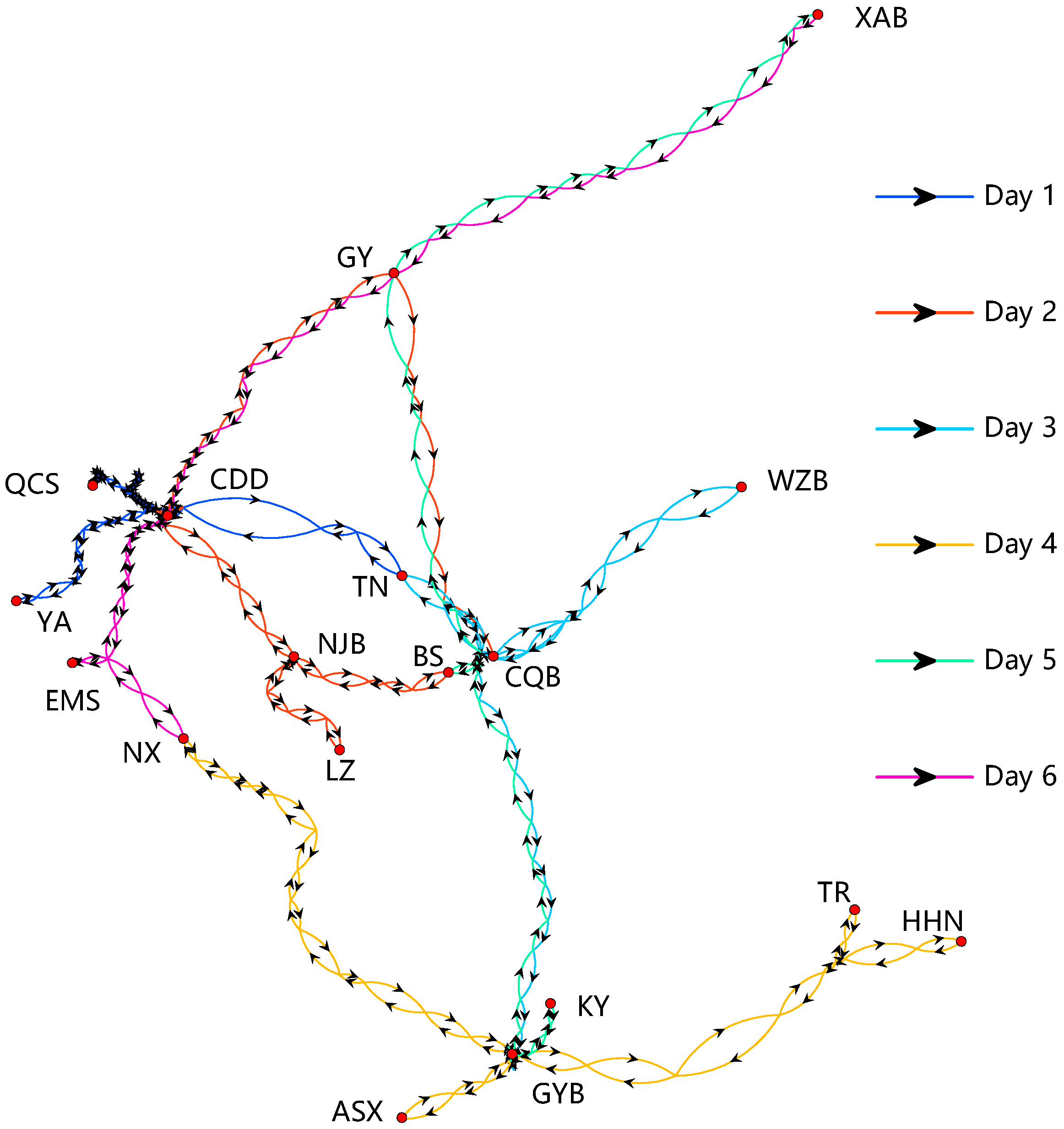
Multi-day inspection paths for a CIT are used as the test experiments, as shown in Figure 8 and

Table 4. Information about major stations on the inspection paths of the experiments.

Days	Inspection Paths
Day 1	CDD → AJ → PXX → PZ → PXX → LDGY → QCS → AJ → CDX → YA → CD → SBT → SN → TN → SN → CDD
Day 2	CDD → NJB → BS → NJB → LZ → NJB → CDD → GY → NCB → CQB
Day 3	CQB → WZB → CQB → TN → CQX → GYB → GY → GYB
Day 4	GYB → ASX → GYB → NX → GYB → TRN → TR → TRN → HHN → GYD
Day 5	GYD → CQX → BS → SPB → NCB → GY → XAB
Day 6	XAB → GY → CDD → LS → EMS → LS → NX → CDD

below. The information on the capacity-saturated periods at each station is shown in

Table 5. Information on station capacity-saturated periods in the test (partial).

No.	Station	Station Capacity-Saturated Periods
1	XP	[335, 363], [371, 379], [395, 403], [412, 496], [498, 538], [545, 710], [717, 736], [742, 766], [770, 823], [827, 877], [879, 946], [948, 968], [977, 997], [1000, 1067], [1072, 1090], [1093, 1110], [1113, 1138], [1140, 1160], [1162, 1187], [1189, 1212], [1225, 1235], [1240, 1248], [1256, 1285], [1291, 1310], [1320, 1328], [1336, 1359], [1382, 1390]
2	ZYB	[461, 463], [477, 480], [484, 484], [534, 537], [621, 624], [671, 671], [1252, 1252]
3	JYB	[564, 573], [593, 601], [639, 654], [672, 682], [702, 745], [749, 763], [777, 790], [815, 824], [861, 869], [875, 884], [899, 914], [963, 971], [987, 1000], [1027, 1035], [1061, 1070], [1075, 1087], [1089, 1098], [1287, 1295]
4	SLJC	[543, 544], [629, 634], [713, 721], [723, 731], [733, 737], [774, 782], [872, 875], [946, 948], [1021, 1023], [1045, 1045], [1088, 1092], [1195, 1197], [1199, 1207]
……	……	……

. The CIT used in the example has a speed class of 300 km/h, the earliest check-in and latest check-out times of the day are 8:00 and 20:00 respectively, and the minimum turnaround time is taken to be 15 min.

5.2. Analysis of Results

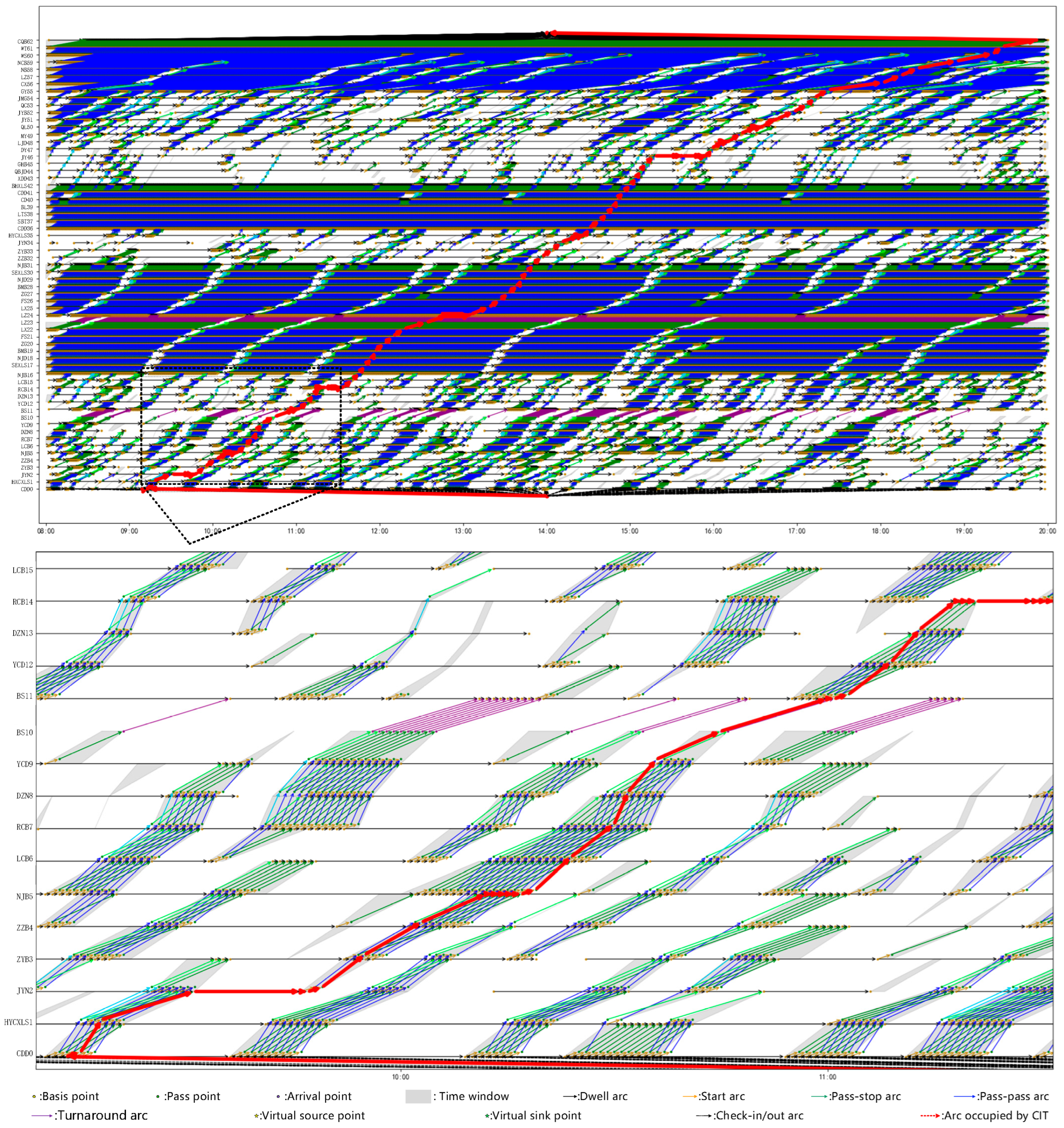
The experiment is based on PyCharm (21.0.5) IDE, using Python 3.7 programming language, and the CIT train line is added for each day’s inspection path. The computing platform is a personal computer with Intel(R) Core(TM) i7-9700K CPU @ 3.60 GHz and 16 GB of RAM. The results are shown in

Table 6. Comparative analysis of the quality of the inspection plan before and after optimization.

Day	No. of Turnaround Stations	Before Optimization					After Optimization
		Check-In Time	Check-Out Time	Total Inspection Duration	No. of Stops	No. of Capacity-Saturated Conflicts	Check-In Time	Check-Out Time	Total Inspection Duration	No. of Stops
Day 1	5	8: 10	19: 42	692 min	19	2	8: 45	19: 50	665 min	8
Day 2	2	8: 02	19: 57	715 min	19	1	9: 13	19: 53	640 min	11
Day 3	5	8: 03	20: 00	717 min	12	0	8: 13	19: 42	689 min	6
Day 4	6	8: 00	19: 51	711 min	19	0	8: 07	19: 49	702 min	14
Day 5	3	8: 00	18: 26	626 min	8	0	8: 05	18: 21	616 min	5
Day 6	3	8: 05	19: 02	657 min	18	1	9: 06	19: 02	596 min	10

. The feasible event arc network and CIT train line are visualised for the second day, as shown in Figure 9.

In the experiment, the primary objective is to minimize the number of stops, and under this premise, the daily inspection duration is compressed as much as possible, so the weights of each type of arc are taken as ${\lambda }^1=0.001, {\lambda }^2=0$, ${\lambda }^3, {\lambda }^4, {\lambda }^5=1$. From the comparison before and after optimization, it can be observed that the proposed method significantly reduces the number of CIT stops and eliminates station capacity conflicts. As shown in Table 6, the total number of CIT stops over the six experimental days decreases from 95 before optimization to 54 after optimization. Therefore, the reduction ratio of non-full-speed inspection sections is calculated as (95−54)/95 × 100% = 43.16%. In addition, the total number of station capacity conflicts is reduced from 4 to 0, indicating that the optimized CIT paths satisfy the station capacity constraints. The total inspection duration is also reduced from 4118 min to 3908 min, corresponding to a total reduction of 210 min. For individual days, the inspection duration is reduced by up to 75 min, as observed on Day 2. Therefore, the optimized plan improves the proportion of full-speed inspection sections while maintaining timetable feasibility.

5.3. Analysis of Solving Time

The experimental process recorded the time consumption for each step in detail, as shown in

Table 7. Analysis of time consumed in sub-solution steps.

Day	No. of Section	Time Consumed (s)
		Step 1	Step 2	Step 3	Step 4	Total Time
Day 1	77	0.26	225.21	48.37	1755.12	2028.96
Day 2	60	0.21	50.49	32.84	642.13	725.67
Day 3	43	0.15	25.24	17.76	314.56	357.72
Day 4	60	0.21	57.58	38.99	621.65	718.44
Day 5	51	0.20	50.87	22.50	564.81	638.38
Day 6	53	0.18	32.53	32.58	422.12	487.41

. Analyses reveal a positive correlation between the time taken for each algorithmic step and the number of sections, with time consumption in Steps 2 and 4 increasing exponentially as the number of sections grows. Further analysis of time consumption distribution indicates that Step 4 is the most time-intensive. This is due to the requirement to assess the in-degree and out-degree of each arc, an operation that must be iteratively performed over multiple cycles. Therefore, the main computational bottleneck of the proposed method lies in FEAN construction and network simplification rather than in the final shortest path search.

In theory, iterations should continue until no invalid arcs remain for deletion; however, due to time constraints, only two deletion cycles were conducted in the experiment. The first two cycles remove the majority of invalid arcs, significantly reducing the feasible event-arc network. The resulting network retains only a few invalid arcs (a small number of which can be observed in Figure 9), but this has minimal impact on subsequent applications of the Dijkstra algorithm. Future applications can further improve computational efficiency by adopting more efficient graph data structures and indexing mechanisms for node-degree calculation, invalid-arc identification, and arc deletion. In addition, event-arc generation and feasibility checking for different sections can be parallelized because these operations are largely independent before path continuity is checked.

It should be noted that the computation times reported in Table 7 cover the complete experimental procedure, including station space–time discretization, interval event-arc generation, station capacity processing, and network simplification. In practical railway timetable planning, these network construction steps do not need to be repeatedly performed during the online decision-making stage. Since the passenger train timetable, headway requirements, and station capacity-saturated periods are known in advance, the corresponding feasible event arc network can be constructed and stored through offline preprocessing. On this basis, the online task for timetable planners or dispatchers is reduced to solving a shortest path problem on the preprocessed FEAN, which can be completed within seconds. Therefore, although the full network construction procedure requires several minutes to tens of minutes in the experimental environment, the actual online response time is acceptable for practical CIT timetable planning and adjustment applications.

To further quantify the effect of infeasible-arc deletion and network simplification, the number of invalid event arcs removed during the construction of the feasible event arc network was recorded. During the iterative event-arc supplementation process, each newly generated event arc is immediately checked against the corresponding departure/pass and arrival/pass time windows. The experimental records show that approximately 10% of the newly supplemented event arcs are identified as infeasible and removed during this feasibility-screening process. After station capacity processing, two additional invalid-arc deletion cycles are conducted to further simplify the network. As shown in

Table 8. Reduction in invalid event arcs during network simplification.

Day	Event Arcs After Interval-Event Processing	Invalid Arcs Deleted in Simplification	Arc Reduction Ratio
Day 1	173,254	4672	2.70%
Day 2	110,500	3445	3.12%
Day 3	91,869	2674	2.91%
Day 4	105,284	4529	4.30%
Day 5	104,330	2677	2.57%
Day 6	74,740	4076	5.45%
Average	109,996	3679	3.34%

, these two cycles remove 2674–4672 invalid event arcs across the six experimental days, corresponding to an arc reduction ratio of 2.57–5.45%. On average, 3679 invalid event arcs are removed, with an average reduction ratio of 3.34%. These results demonstrate that infeasible-arc deletion and network simplification effectively reduce redundant event arcs before applying the shortest path algorithm.

6. Conclusions

The proposed approach improves the utilization of existing railway capacity for inspection operations, enhances infrastructure maintenance efficiency, and supports the sustainable and reliable operation of high-speed railway systems. To minimize the number of CIT stops, achieve full-speed inspections across more sections, and ensure timetable feasibility, this study carefully considers station capacity saturation constraints. Under these conditions, we investigate the model and solution approach for CIT scheduling, constructing a nonlinear mixed-integer programming model. To address the challenge of nonlinear constraints, we apply event–activity network concepts, using time windows to determine the feasibility of various event arcs. We then improve the existing space–time network construction method by identifying all arcs that meet the time window and operational rules, forming a feasible event-arc network and transforming the original problem into an equivalent shortest path problem. This processing procedure encompasses four main stages: station space–time discretization, interval operation event processing, station capacity handling, and network simplification. To facilitate the solution process, we also develop a train line addition model based on the feasible event-arc network, allowing for the expression of different optimization objectives by adjusting the weights of various event arcs. The testing results indicate that all station capacity conflicts are resolved, inspection duration is reduced, the number of stops is optimized, and the number of non-full-speed inspection sections is decreased by 43.16%. Moreover, the solution time is acceptable for practical applications.

Although the proposed method is developed and tested for planned CIT path scheduling, its application is not limited to this specific case. The key premise of the method is that the existing train paths are treated as fixed or only slightly adjusted, while the task is to find a feasible path for an additional or adjusted train within the remaining timetable capacity. Therefore, the framework can also provide methodological support for temporary additional train path scheduling, minor delay recovery, and timetable capacity assessment. For example, when temporary passenger or freight train paths need to be added without modifying the published passenger timetable, the time windows and station capacity-saturated periods can be derived from the existing timetable, and a feasible additional path can then be searched on the constructed FEAN. Similarly, when a CIT path or a small number of train paths need to be adjusted due to limited delays, the corresponding time windows can be updated, and the feasible path can be regenerated by solving the shortest path problem on the updated network.

However, for severe disruption management scenarios involving large-scale train cancellations, rerouting, changes in platform-track assignment, or simultaneous adjustment of multiple passenger trains and CIT paths, the current framework requires further extension. In such cases, the fixed-timetable assumption may no longer hold, and the FEAN-based model should be integrated with real-time train rescheduling, station route assignment, and rolling-horizon optimization methods. In addition, although stop reduction is selected as the primary objective in this study because of its direct relationship with full-speed inspection and data quality, other operational objectives, such as inspection duration, timetable robustness, energy consumption, and operational margins, can be further incorporated into the proposed framework through multi-objective optimization or adjusted event-arc weights.

The scalability of the proposed framework also deserves further investigation. For larger railway networks and more complex inspection paths, the FEAN construction logic remains applicable, but the number of event arcs may increase rapidly as the number of stations, sections, and fragmented feasible time windows grows. Therefore, more efficient graph storage structures, parallel event-arc generation, and local network updating strategies are needed to improve computational efficiency. For multiple CITs, additional coupling constraints related to shared infrastructure capacity, station occupation, inspection task allocation, and inter-train conflicts should be considered. In this case, the current single-CIT shortest path formulation can be extended to a multi-source and multi-sink network flow model, an iterative path generation framework, or a coordinated multi-train optimization model. These extensions will be important directions for future research.

References

1. Garmabaki, A.H.S.; Thaduri, A.; Famurewa, S.; Kumar, U. Adapting Railway Maintenance to Climate Change. Sustainability 2021, 13, 13856. [Google Scholar] [CrossRef] [Scilit]
2. Xu, M.; Shuai, B.; Wang, X.; Li, J.; Huang, W. A Two-Stage Optimization Approach for Inspection Plan Formulation of Comprehensive Inspection Train: The China Case. Comput. Ind. Eng. 2021, 159, 107465. [Google Scholar] [CrossRef] [Scilit]
3. Wang, J.; Zhao, W.; Liu, C.; Huang, Z. A System Optimization Approach for Trains’ Operation Plan with a Time Flexible Pricing Strategy for High-Speed Rail Corridors. Sustainability 2023, 15, 9556. [Google Scholar] [CrossRef] [Scilit]
4. Burdett, R.L.; Kozan, E. Techniques for Inserting Additional Trains into Existing Timetables. Transp. Res. Part B Methodol. 2009, 43, 821–836. [Google Scholar] [CrossRef] [Scilit]
5. Cacchiani, V.; Caprara, A.; Toth, P. Scheduling Extra Freight Trains on Railway Networks. Transp. Res. Part B Methodol. 2010, 44, 215–231. [Google Scholar] [CrossRef] [Scilit]
6. Gao, Y.; Kroon, L.; Yang, L.; Gao, Z. Three-Stage Optimization Method for the Problem of Scheduling Additional Trains on a High-Speed Rail Corridor. Omega 2018, 80, 175–191. [Google Scholar] [CrossRef] [Scilit]
7. Jiang, F.; Cacchiani, V.; Toth, P. Train Timetabling by Skip-Stop Planning in Highly Congested Lines. Transp. Res. Part B Methodol. 2017, 104, 149–174. [Google Scholar] [CrossRef] [Scilit]
8. Tan, Y.-Y.; Li, Y.-X.; Wang, R.-X. Scheduling Extra Train Paths into Cyclic Timetable Based on the Genetic Algorithm. IEEE Access 2020, 8, 102199–102211. [Google Scholar] [CrossRef] [Scilit]
9. Flier, H.; Graffagnino, T.; Nunkesser, M. Scheduling Additional Trains on Dense Corridors. In Proceedings of the Experimental Algorithms; Vahrenhold, J., Ed.; Springer: Berlin/Heidelberg, Germany, 2009; pp. 149–160. [Google Scholar]
10. Ingolotti, L.; Barber, F.; Tormos, P.; Lova, A.; Salido, M.A.; Abril, M. An Efficient Method to Schedule New Trains on a Heavily Loaded Railway Network. In Proceedings of the Advances in Artificial Intelligence—IBERAMIA 2004; Lemaître, C., Reyes, C.A., González, J.A., Eds.; Springer: Berlin/Heidelberg, Germany, 2004; pp. 164–173. [Google Scholar]
11. Liu, Y.; Cao, C.; Feng, Z.; Zhou, Y. A Cost and Passenger Responsible Optimization Method for the Operation Plan of Additional High-Speed Trains in a Peak Period. J. Adv. Transp. 2020, 2020, e3602727. [Google Scholar] [CrossRef] [Scilit]
12. Ljunggren, F.; Persson, K.; Peterson, A.; Schmidt, C. Railway Timetabling: A Maximum Bottleneck Path Algorithm for Finding an Additional Train Path. Public Transp. 2021, 13, 597–623. [Google Scholar] [CrossRef] [Scilit]
13. Gao, R.; Niu, H. Study on Additional Train Timetable Algorithm in Flexible Manner Based on ADMM Approach. J. China Railw. Soc. 2021, 43, 21–29. [Google Scholar]
14. Tan, Y.; Jiang, Z. A Branch and Bound Algorithm and Iterative Reordering Strategies for Inserting Additional Trains in Real Time: A Case Study in Germany. Math. Probl. Eng. 2015, 2015, e289072. [Google Scholar] [CrossRef] [Scilit]
15. Jiang, F.; Ni, S.; Lv, H. A High-Speed Railway New-Added Train Timetable Partial Adjustment Model Based on Lagrangian Relaxation. J. Transp. Syst. Eng. Inf. Technol. 2018, 18, 163–170. [Google Scholar] [CrossRef]
16. Liu, Y.; Cao, C. A Multi-Objective Train Operational Plan Optimization Approach for Adding Additional Trains on a High-Speed Railway Corridor in Peak Periods. Appl. Sci. 2020, 10, 5554. [Google Scholar] [CrossRef] [Scilit]
17. Nachtigall, K. Periodic Network Optimizationi and Fixed Interval Timetables. Habilitation Thesis, Universität Hildesheim, Hildesheim, Germany, 1999. [Google Scholar]
18. Dollevoet, T.; Huisman, D.; Schmidt, M.; Schöbel, A. Delay Management with Rerouting of Passengers. Transp. Sci. 2012, 46, 74–89. [Google Scholar] [CrossRef] [Scilit]
19. Liu, X.; Zhou, M.; Dong, H.; Wu, X.; Li, Y.; Wang, F.-Y. ADMM-Based Joint Rescheduling Method for High-Speed Railway Timetabling and Platforming in Case of Uncertain Perturbation. Transp. Res. Part C Emerg. Technol. 2023, 152, 104150. [Google Scholar] [CrossRef] [Scilit]
20. Sparing, D.; Goverde, R.M.P. A Cycle Time Optimization Model for Generating Stable Periodic Railway Timetables. Transp. Res. Part B Methodol. 2017, 98, 198–223. [Google Scholar] [CrossRef] [Scilit]
21. Yin, J.; Ren, X.; Su, S.; Yan, F.; Tao, T. Resilience-Oriented Train Rescheduling Optimization in Railway Networks: A Mixed Integer Programming Approach. IEEE Trans. Intell. Transp. Syst. 2023, 24, 4948–4961. [Google Scholar] [CrossRef] [Scilit]
22. D’Ariano, A.; Pranzo, M.; Hansen, I.A. Conflict Resolution and Train Speed Coordination for Solving Real-Time Timetable Perturbations. IEEE Trans. Intell. Transp. Syst. 2007, 8, 208–222. [Google Scholar] [CrossRef] [Scilit]
23. D’Ariano, A.; Corman, F.; Pacciarelli, D.; Pranzo, M. Reordering and Local Rerouting Strategies to Manage Train Traffic in Real Time. Transp. Sci. 2008, 42, 405–419. [Google Scholar] [CrossRef] [Scilit]
24. D’Ariano, A. Innovative Decision Support System for Railway Traffic Control. IEEE Intell. Transp. Syst. Mag. 2009, 1, 8–16. [Google Scholar] [CrossRef] [Scilit]
25. Corman, F.; D’Ariano, A.; Pacciarelli, D.; Pranzo, M. A Tabu Search Algorithm for Rerouting Trains during Rail Operations. Transp. Res. Part B Methodol. 2010, 44, 175–192. [Google Scholar] [CrossRef] [Scilit]
26. Xu, P.; Corman, F.; Peng, Q.; Luan, X. A Train Rescheduling Model Integrating Speed Management during Disruptions of High-Speed Traffic under a Quasi-Moving Block System. Transp. Res. Part B Methodol. 2017, 104, 638–666. [Google Scholar] [CrossRef] [Scilit]
27. Caprara, A.; Fischetti, M.; Toth, P. Modeling and Solving the Train Timetabling Problem. Oper. Res. 2002, 5, 851–861. [Google Scholar] [CrossRef] [Scilit]
28. Zhang, Y.; Peng, Q.; Yao, Y.; Zhang, X.; Zhou, X. Solving Cyclic Train Timetabling Problem through Model Reformulation: Extended Time-Space Network Construct and Alternating Direction Method of Multipliers Methods. Transp. Res. Part B Methodol. 2019, 128, 344–379. [Google Scholar] [CrossRef] [Scilit]
29. Liao, Z.; Li, H.; Miao, J.; Corman, F. Railway Capacity Estimation Considering Vehicle Circulation: Integrated Timetable and Vehicles Scheduling on Hybrid Time-Space Networks. Transp. Res. Part C Emerg. Technol. 2021, 124, 102961. [Google Scholar] [CrossRef] [Scilit]
30. Higgins, A.; Kozan, E.; Ferreira, L. Optimal Scheduling of Trains on a Single Line Track. Transp. Res. Part B Methodol. 1996, 30, 147–161. [Google Scholar] [CrossRef] [Scilit]
31. Huang, Y.; Mannino, C.; Yang, L.; Tang, T. Coupling Time-Indexed and Big-M. Formulations for Real-Time Train Scheduling during Metro Service Disruptions. Transp. Res. Part B Methodol. 2020, 133, 38–61. [Google Scholar] [CrossRef] [Scilit]
32. Zhao, X.; Li, D.; Bao, X. A Deep Reinforcement Learning Approach for Integrated Optimization of Train Scheduling and Rolling Stock Circulation Planning. Comput. Ind. Eng. 2026, 213, 111784. [Google Scholar] [CrossRef] [Scilit]
33. Pan, J.; Liu, R.; Lin, Z.; Zhan, S. Scheduling Extra Trains to an Existing Timetable along a Railway Corridor: An ADMM-Based Optimisation Approach. Expert Syst. Appl. 2026, 319, 132033. [Google Scholar] [CrossRef] [Scilit]
34. Zhao, T.; Zhang, Y.; Bešinović, N.; Zhan, S.; Zhang, S.; Peng, Q. A Lagrangian Relaxation-Based Approach for Integrated Optimization of Line Planning and Additional Trains Scheduling. Comput. Ind. Eng. 2026, 212, 111667. [Google Scholar] [CrossRef] [Scilit]
35. Mannino, C.; Nakkerud, A. Optimal Train Rescheduling in Oslo Central Station. Omega 2023, 116, 102796. [Google Scholar] [CrossRef] [Scilit]
36. Ye, X.; Du, Y.; Yang, H.; Pan, J.; Ni, S.; Chen, D. Collaborative Optimization of Train Timetabling with Maintenance Window Setting and Maintenance Scheduling Considering Fluctuating Daily Train Volumes and Dynamic Maintenance Demands. Transp. Res. Part C Emerg. Technol. 2026, 185, 105552. [Google Scholar] [CrossRef] [Scilit]
37. Guo, J.; Wang, Y.; Guo, X.; Guo, J.; D’Ariano, A.; Bosi, T.; Zhang, Y. Structure-Optimized Deep Forest Model for Railway Port Container Reloading Time Prediction: A Hybrid Integer Programming and Bayesian Optimization Approach. Adv. Eng. Inform. 2026, 71, 104309. [Google Scholar] [CrossRef] [Scilit]
38. Zhan, Y.; Zhang, X.; Ye, M. Demand-Driven Integrated Optimization of Train Route, Timetable and Rolling Stock Scheduling in Urban Rail Transit: A Flexible Composition Strategy for in-Service and Additional Trains. Transp. Res. Part E Logist. Transp. Rev. 2026, 212, 104959. [Google Scholar] [CrossRef] [Scilit]
39. Guo, J.; Wang, Y.; Chen, Z.-S.; Chiclana, F.; Pedrycz, W. Enhancing Multivariate Time Series Forecasting for Container Reloading Operations: An Improved Adaptive Multi-Granularity Cascade Forest Model Integrating. Transp. Res. Part E Logist. Transp. Rev. 2026, 211, 104847. [Google Scholar] [CrossRef] [Scilit]
Figure 1. Three-level planning framework for CIT operations.
Sustainability 18 06505 g001
Figure 2. Analysis of the departure–arrival type association constraints.
Sustainability 18 06505 g002
Figure 3. Characterisation of the time window structure.
Sustainability 18 06505 g003
Figure 4. The process of constructing the space–time network.
Sustainability 18 06505 g004
Figure 5. The process of station space–time discretization: (a) discretization of general stations; (b) discretization of turnaround station; (c) construction of turnaround arcs between the virtual arrival points and basis points; (d) simplified result after removing infeasible turnaround arcs and isolated virtual arrival points.
Sustainability 18 06505 g005
Figure 6. The process of interval operation events: (a) determination of valid basis points according to the departure/pass time window and addition of start arcs; (b) addition of pass–stop arcs and pass–pass arcs from the passing points activated by the start arcs; (c) identification of infeasible pass–stop arcs whose end points fall outside the arrival/pass time window; (d) identification of infeasible pass–pass arcs whose end points fall outside the arrival/pass time window; (e) further addition of pass–stop arcs and pass–pass arcs from valid pass points with out-degree 0; (f) final feasible event arc network after deleting infeasible arcs.
Sustainability 18 06505 g006
Figure 7. The process of network simplification: (a) deletion of invalid arcs according to the out-degree values of the arc endpoints; (b) deletion of invalid passing points according to the in-degree values and simplification of redundant basic points with both in-degree and out-degree equal to 1; (c) addition of the virtual source point, virtual sink point, check-in arcs, and check-out arcs to obtain the streamlined feasible event arc network; (d) shortest path result corresponding to the feasible train line with the highest technical speed.
Sustainability 18 06505 g007
Figure 8. Inspection paths of the experiments.
Sustainability 18 06505 g008
Figure 9. Example of adding CIT train line approach based on space–time network (Day 2).
Sustainability 18 06505 g009