Environmental Tax Races in a Decentralised System: Evidence of Regional Interaction in Climate Policy

Abstract

Environmental taxation constitutes a key instrument of climate policy and plays an increasingly important role in decentralised governance systems. Using Spain as an empirical setting characterised by high fiscal decentralisation and pronounced territorial heterogeneity, we analyse the determinants of regional environmental taxation, accounting for both internal regional conditions and cross-regional policy interaction. Employing spatial panel econometric techniques, we provide robust evidence of spatial interaction and temporal persistence in regional environmental taxation at both the intensive and extensive margins. We also find that regional environmental taxation depends not only on domestic economic, institutional, and political characteristics, but also on those of neighbouring regions. These patterns are consistent with key theoretical mechanisms in fiscal federalism and public economics, including tax competition, yardstick competition, the double dividend hypothesis, NIMBY-type responses, and development–environment dynamics. Fur-ther analysis at the intensive margin reveals adjustment patterns consistent primarily with upward dynamics, although some evidence of downward responses is also found. In particular, upward adjustments appear to be more systematic, while downward responses are limited to regions with relatively lower environmental taxation. This asymmetry sug-gests that competitive pressures do not operate uniformly across jurisdictions. From a sustainability and governance perspective, the findings show that environmental tax policies in decentralised systems are shaped by strategic inter-regional interdependence, influencing the trajectories of regional sustainability transitions rather than reflecting isolated policy choices.

1. Introduction

In the context of accelerating climate change and the growing prominence of environmental policy objectives, regions have become key arenas for the design and implementation of climate policies. In decentralised systems of governance, subnational governments play a central role in contributing to these objectives through a combination of policy instruments, including environmental regulation, public investment, and environmental taxation. These instruments are increasingly viewed not only as tools for internalising environmental externalities, but also for addressing environmental challenges.

Subnational governments do not design their policies in isolation; rather, they take into account the policy choices adopted by other jurisdictions. In the field of taxation, these interactions have been analysed mainly for capital and income taxes, reflecting governments’ desire to attract capital and firms (See [1,2,3]) and/or to please voters, in order to get re-elected, since citizens pay attention to the type of income and spending of analogous jurisdictions to assess the performance of their own rulers ([4,5,6,7]). This literature has also considered additional dimensions such as budget constraints, welfare considerations, differences in regional costs, and even vertical interactions [8,9].

A closely related strand of research has examined interjurisdictional interaction in environmental regulation, particularly in contexts characterised by environmental externalities and pollution spillovers. This literature can be broadly classified into three main strands according to the direction of the relationship identified. First, a substantial body of work highlights the potential risk of a “race to the bottom”, whereby jurisdictions relax environmental standards in order to attract economic activity (e.g., [5,10,11,12,13]). Empirical evidence supporting this behaviour has been documented for the United States [14,15] and for China [16,17]. Second, another strand of the literature argues that these concerns may be overstated, since burden imposed by regulations is usually a negligible part of firms’ total costs, and in consequence there is little incentive for industries to change location according to differences in the cost of environmental regulations (although there is also empirical evidence for such delocalisation (e.g., [18])). This perspective is reflected in both theoretical [19,20] and empirical studies [21,22,23] that find no systematic evidence of regulatory relaxation. More recent contributions also suggest that the interaction between environmental regulation and tax competition does not necessarily lead to pollution havens (e.g., [24]). Third, a growing body of work provides evidence that has been interpreted as consistent with a “race to the top”, where competition between jurisdictions may improve environmental quality and discourage highly polluting activities (e.g., [25,26,27,28]). In addition, some literature affirms that, given the heterogeneity of regions, races to the bottom and to the top may coexist in the environmental regulation of jurisdictions (e.g., [29,30,31]) (however, there are also studies which find no evidence for spatial interaction (e.g., [32])). From a sustainability perspective, these contrasting dynamics are crucial, as they imply that interjurisdictional competition can either undermine or reinforce subnational contributions to climate mitigation and sustainable development goals.

Despite the growing use of environmental taxation as a core policy instrument of climate policy, empirical analyses of interjurisdictional interaction in environmental taxation remain scarce. Existing empirical evidence is limited to a small number of studies. Levinson [33] obtains a positive association (1.1) between the rates of taxes on hazardous waste deposits in the USA for the period 1989–1995. To do this, he uses a two-stage least squares estimator (2SLS) and estimates the taxation of a state depending on that of its neighbouring states, weighted with a spatial weights matrix. Ashworth et al. [34], within the framework on the diffusion of an innovation or new policy [35,36,37], analyse for the first time the decision to introduce an environmental tax for Flemish municipalities in the period 1991–1999, using a discrete time hazard logit model. They find that the probability of a municipality introducing an environmental tax is higher if its geographical and ideological neighbours already have one. Zhang [38] extends this diffusion perspective to the analysis of environmental taxation in an international context, focusing on a sample of 29 OECD countries. Renard and Xiong [39] find a positive relationship (with coefficients ranging from 0.069 to 1.9) among the environmental tax revenues, measured in terms of industrial GDP, of 30 Chinese provinces for the period 2004–2009. For this estimate, they use a two-stage least squared instrumental variables (2SLS-IV) method and, like Levinson [33], a spatial weights matrix.

A related strand of the literature has examined convergence in environmental taxation, suggesting that tax levels may evolve towards similar patterns across countries, partly driven by catch-up dynamics and spatial spillovers, although without directly addressing interjurisdictional interaction in tax-setting behaviour (e.g., [40,41]).

Recent contributions have also analysed the effects of environmental policies within the European Union, particularly in the context of the EU Emissions Trading Scheme, highlighting how such policies interact across jurisdictions and how overlapping national measures can affect aggregate outcomes (e.g., [42,43,44,45]). While most of this literature does not focus directly on environmental taxation, it nonetheless provides relevant insights into interjurisdictional policy interaction in multi-level governance settings. In parallel, although also in contexts different from environmental taxation, methodological advances have introduced new approaches to identifying policy spillovers, including machine learning techniques and related causal inference methods (e.g., [46,47]).

Taken together, these strands of research indicate that, while interjurisdictional interaction is well established in the context of environmental regulation, comparatively little is known about how such interaction operates in the domain of environmental taxation. This gap is especially relevant given the increasing reliance on environmental taxes as policy instruments in environmental governance. Insights from the literature on tax competition and environmental policy point to several mechanisms through which spatial interdependence may arise in subnational environmental taxation, including competition for mobile capital and industrial activity, strategic tax-setting aimed at preserving regional competitiveness, policy emulation under yardstick competition, and the management of environmental externalities that transcend administrative borders. These mechanisms make regional environmental taxation a fertile ground for spatial interaction, particularly in decentralised systems such as Spain.

Against this background, this paper examines the nature of spatial interaction in the environmental tax effort of Spanish regions and, in particular, whether such interaction is consistent with upward or downward adjustment dynamics, often associated in the literature as race to the top or race to the bottom processes. Using Spain as an empirical setting characterised by pronounced territorial heterogeneity and extensive fiscal decentralisation, we analyse the environmental taxation experience of the 17 autonomous communities over the period 2005–2019, through a dynamic spatial econometric model.

Spain provides a particularly suitable empirical setting for examining these issues. It is a highly decentralised country with three levels of government (central, regional, and local), in which environmental damage is regulated through centrally established standards, based on both European and national legislation, while implementation and monitoring are largely carried out at the regional level. As a result, regional governments enjoy considerable autonomy in shaping their environmental policies, despite the presence of federal-level legislation. In practice, Spanish regions have made extensive use of environmental taxes, not only as instruments to address environmental damage but also as sources of public revenue. This multi-level governance framework, together with the fiscal autonomy of regions to introduce their own taxes, creates a context of significant territorial heterogeneity in environmental taxation. These features make Spain an especially appropriate setting to analyse interregional interaction in environmental tax policy. Therefore, our study contributes to addressing this empirical gap and provides new evidence from a European context on this phenomenon. In this framework fragmented or strategically driven regional tax policies may either hinder or reinforce coherent environmental policy and regional development.

While environmental taxation is often considered a relevant instrument for sustainability-oriented governance, this paper does not assess environmental outcomes, but instead focuses on spatial interaction of environmental tax policies across regions within a decentralised fiscal framework. In particular, it goes beyond the mere identification of spatial dependence to examine patterns of interregional interaction that may be consistent with different underlying mechanisms. To this end, it analyses how regional environmental taxation at both the intensive margin—related to tax effort—and the extensive margin—related to the decision to adopt environmental taxes—are shaped by interregional dynamics rather than by isolated policy choices.

The remainder of the paper is structured as follows: Section 2 provides context by reviewing the environmental taxes of the Spanish regions. Section 3 presents the empirical model and hypotheses. Section 4 discusses the results, while Section 5 provides a sensitivity analysis. Section 6 explores asymmetrical behaviour in spatial interaction. The paper concludes with a section of concluding remarks.

2. Study Framework

In Spain, environmental tax revenues reached 19.75 billion euros in 2020, which represented 1.75% of GDP, but according to EUROSTAT, it was below the European Union (EU) average of 2.24% of GDP. Although the environmental tax policies of each member state vary widely, as each one has a different definition of what an environmental tax is, across EU countries as a whole, most of this revenue (78%) comes from taxes on energy, while taxes on transport represent 19%, and taxes relating to environmental damage just 3.2%. However, energy taxes in Spain represent a slightly higher percentage (82.9%). This is established in the Report on energy taxation, carbon pricing and energy subsidies, which the European Court of Auditors presented in early 2022.

Of the three levels of government in Spain, only the central and regional levels have made use of environmental taxes as an economic instrument to incentivise changes in behaviour considered to be positive for the environment. Local governments have gone no further than setting a tax allowance in some local taxes to encourage clean energy use.

At the state level, the role of environmental taxes, until a few years ago, was fairly limited [48], as until 2012 Spain collected only the Special Hydrocarbon Tax, the Electricity Tax, and the Tax on Certain Means of Transport. In 2012 Spain approved the Tax on the Production of Spent Nuclear Fuel and Radioactive Waste, the Tax on the Storage of Spent Nuclear Fuel and Radioactive Waste, the Tax on the Value of Electricity Production, and the Tax on the Use of Inland Water for Electricity Production. In 2013 it introduced the Tax on Fluorinated Greenhouse Gases. In 2023 a Tax on Waste Disposal in Landfills and Incineration, a Special Tax on Single-Use Packaging, and a temporary Energy Levy came into force.

Meanwhile, legislative activity at the regional level has been more intense. It should be borne in mind that the Spanish regions or autonomous communities have broad autonomy in their tax policies. They have the regulatory power not only to modify the rates of some state taxes, whose collection is totally or partially ceded to them, and to establish their own rebates on them, but they can also introduce new taxes, as long as these ‘own’ taxes do not levy items already taxed by the central government, as stipulated in the Organic Law on the Financing of Autonomous Communities (LOFCA). To get around this restriction, the Spanish regions have approved taxes on some form of pollution: on emissions, waste (as the new state Tax on Waste, in force since 2023, taxes items already taxed by the regions, these regional taxes are no longer in force and have been replaced by the state tax, with the same structure and terms, throughout the country), water treatment, large shopping centres, electricity transportation, and so on. In fact, each Spanish region has established the environmental taxes it has deemed appropriate, regulating them as it has wished, hence the term ‘own’ environmental taxes.

The result of this tax autonomy is the enormous diversity of the Spanish regions’ taxation system. As shown in

Table A1. Green taxes by region and year of introduction.

	Emissions	Waste						Water			Energy			Territory
	Emissions	Municipal Waste Incineration	Municipal Waste Deposit	Construction Waste Deposit	Industrial Waste Deposit	Radioactive Waste Storage	Plastic Bags	Sanitation Levy	Coastal Water Runoff	Reservoir Water Use	Electricity Generation	Fixed Energy Transport and/or Telephony Elements	Wind Power Levy	Cable Cars	Hunting	Mining Tax	Commercial Establishments	Tourist Establishments
Andalusia	2003				2003	2003 *	2010	2010	2003
Aragon	2005							2001		2017		2017		2005 *			2005
Asturias								1994				2010					2002
Balearics		2020	2020					1991										2016
Canary Islands									1994			2012 *					2012 *
Cantabria					2009		2011 *	2002
Castilla y León			2012		2012	2012				2012		2012	2012
Castilla-La Mancha	2000					2000)		2002			2000		2011
Catalonia	2015	2009	2004	2009 *	2014			2000									2000	2011
Autonomous Region of Valencia	2012				2012			1992			2012	2012
Extremadura			2012	2012	2012		2012 *				1998	1998			1991
Galicia	1996							1993		2008			2009			2014
Madrid					2003			1984
Murcia	2005			2005	2005			2000	2005
Navarre			2018	2018	2018			1988									2018
Basque Country								2006
La Rioja					2012			2000				2012

* Later suspended.

of the Annex, the 17 regions have different tax structures (even though 80% of their tax revenue comes from state income and consumption taxes), to such an extent that there are currently around 80 different regional taxes in force in Spain. Most of these regional taxes are environmental in nature, mostly levied on industries, often with growing tax rates according to their pollution levels. This means that environmental taxes are being used as active policy instruments intended to lead to changes in polluter behaviour; furthermore, the link with environmental policy is reinforced because in practically all environmental taxes, their collection must be used to fund regional initiatives to remedy or reduce the environmental damage. However, there is a widespread opinion that the tax collection–environmental purposes relationship is touted as making their adoption less costly politically, when they actually have a revenue-gathering purpose which permits the allocation of resources for other purposes (fungibility effect).

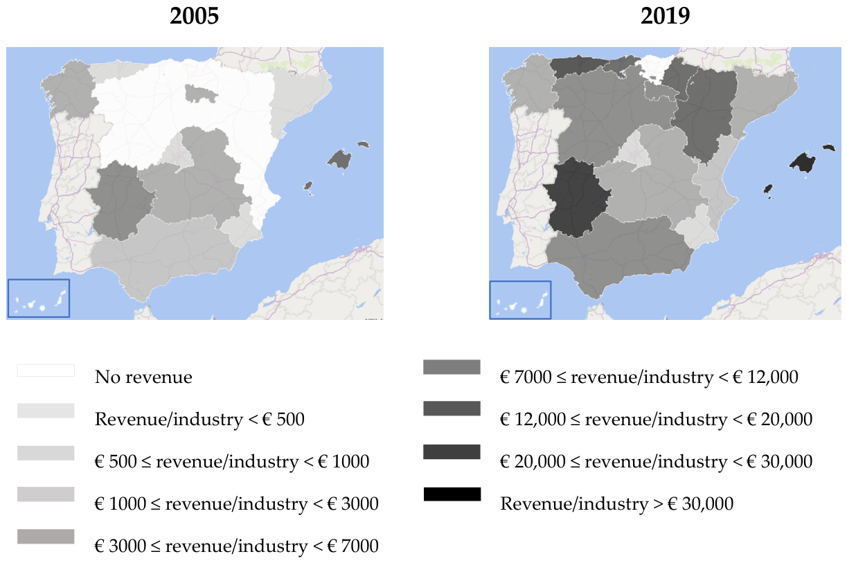
Figure 1 shows a tax revenue map of two moments in time, 2005 and 2019, suggesting several ideas. First, the gradual introduction of environmental taxes by the regions has increased the revenue from these taxes in practically all the regions of Spain. Second, while in 2005 this tax revenue was practically confined to the southern half of the country, by 2019 environmental taxes were in force almost everywhere in Spain, with notably high revenues in the northern regions. And third, in 2019 the central and eastern regions of mainland Spain were producing the lowest revenues from environmental taxes. These data seem to suggest the existence of a spatial correlation in the environmental tax effort of Spanish regions, which we will examine empirically in the next section.

3. Model and Hypothesis

The theoretical model underlying our estimates is the classic tax competition model [49,50], according to which regions compete with each other to attract investment and economic activity by reducing taxes. In this context of tax competition, where regions seek to balance tax revenue with the need to maintain an attractive economic environment, and also considering other relevant theories in the field of taxation and fiscal federalism, such as the double dividend theory [51] or yardstick competition [4], each region i will take decisions regarding its environmental taxation that will depend primarily on the characteristics of that region, such as its environmental problem, regulation, level of development, financial health, and political and demographic circumstances, but also on certain characteristics of its neighbouring regions, such as the severity of their environmental taxation. More recent studies have also used this approach [52,53], although as we mentioned earlier, in the field of environmental taxation, such works are anecdotal.

Our aim in this paper is to explore spatial interdependence in both margins of environmental tax decision-making. Accordingly, the paper first examines whether regional environmental tax policies exhibit spatial interaction at both the intensive margin—related to tax effort—and the extensive margin—related to the decision to adopt environmental taxes. Building on this evidence, the analysis then focuses on the intensive margin to characterise the nature of spatial interaction, assessing whether regional environmental taxation is consistent with upward or downward adjustment dynamics. In line with Woods [14] and Konisky [29], our objective is not to estimate the effects of such interactions, but rather to identify and classify their form.

To do this, we will estimate regional environmental taxes with a dynamic spatial model, using a sample consisting of the 17 Spanish regions in the period 2005–2019. By using a dynamic model, we are considering the possibility that a region’s environmental taxes may depend on those of previous years, given that these taxes are not established for a single year, but are usually implemented on a continuous basis over time. The use of a spatial model enables us to analyse whether the environmental tax policy of a region is affected by the environmental taxes of neighbouring regions (global spatial dependence), by the individual characteristics of the neighbouring regions (local spatial dependence), and even whether there is spatial dependence between omitted variables (spatial dependence in the error term). Additionally, with this model, we can consider the possibility that the spatial dependence continues over time and/or requires time (non-contemporaneous global spatial dependence). Otherwise, we would be assuming that the regions’ environmental tax decisions are simultaneous (contemporaneous), when the reality is that approving a tax in response to one established in a neighbouring region can take some time (usually longer than needed to adopt a certain degree of stringency in regulatory compliance, which could take place contemporaneously), as it requires legislative action.

To capture the spatial dimension, we construct a 17 × 17 spatial weights matrix (W) based on the five geographically closest regions. This proximity matrix is grounded in Tobler’s [54] First Law of Geography—everything is related to everything else, but nearby things are more related than distant things—and provides a simple and exogenous way to capture spatial interdependence across regions. Alternative specifications present limitations in this context. A contiguity matrix in Spain would leave island regions without neighbours, while an inverse distance matrix would assign them negligible weights due to their geographic isolation, artificially limiting their influence in the spatial structure, and would introduce additional parameters and risk overparameterization. Although the geographical position of the island regions may imply relatively weaker spatial linkages, their exclusion would be problematic. These regions belong to the same institutional and fiscal framework as the rest of the autonomous communities and are involved in processes of policy comparison, learning, and diffusion at the national level. In addition, their exclusion would further reduce the degrees of freedom, which is particularly relevant given the limited sample size. Nevertheless, estimations excluding island regions yield qualitatively similar results. To address concerns about arbitrariness, we conducted a robustness analysis using alternative number of neighbours, as well as a placebo matrix. This analysis is presented in Section 5. Weighting schemes based on economic similarity (e.g., industrial structure) may raise identification problems, as they rely on variables closely related to both the dependent variable and the regressors, making it difficult to disentangle genuine spatial interaction effects from underlying structural similarities. Thus, each of the elements, ${\omega }_{ij}$, of the spatial matrix, W, takes the value 1 if region j is one of the five closest to region i, so by definition w_ii = 0 (for simplicity’s sake, we will suppose that the spatial weights matrix is the same as the spatio-temporal weights matrix).

Therefore, the model we will estimate with panel data would have the following general specification:

$$\begin{array}{c}{green\_taxes}_{it}=\rho {\displaystyle {\sum }_{j=1}^{17}}{\omega }_{ij}{green\_taxes}_{jt}+\partial {\displaystyle {\sum }_{j=1}^{17}}{\omega }_{\left(ij\right)t-1}{green\_taxes}_{jt-1}+\gamma {green\_taxes}_{it-1}+\\ {\displaystyle {\sum }_{k=1}^K}{x}_{itk}{\beta }_k+{\displaystyle {\sum }_{s=1}^S}{\displaystyle {\sum }_{j=1}^{17}}{\omega }_{ij}{x}_{jts}{\phi }_s+{\delta }_i+{\tau }_t+u_{it}\end{array}$$

(1)

$$u_{it}=\lambda {\displaystyle {\sum }_{j=1}^{17}}{\omega }_{ij}{u}_{it}+{\epsilon }_{it,}$$

With i = 1,…17, j ≠ i, and t = 2005,…2019.

where the dependent variable, green_taxes_it, captures the environmental tax level of region i in year t, measured as environmental tax revenue relative to the number of industrial firms, which are the main taxpayers of these instruments. We construct this variable using total environmental tax revenue at the regional level, because interregional tax interaction does not necessarily occur within a single tax instrument. The unique qualities of each region may lead each one to focus on a different type of environmental damage, and interregional interaction may therefore take place between different environmental taxes, so that if one region has established an emissions tax, a neighbouring region concerned, for example, with waste generation could be encouraged to establish a tax on waste. Along these lines, Berry and Berry [55] find that the more taxes are established in neighbouring regions, the more likely a given region is to establish a tax, while Fredriksson et al. [56] find evidence of cross-policy interactions between US states in such diverse policies as taxes, spending, and regulation. Accordingly, our dependent variable should be interpreted as a proxy for the average environmental tax burden borne by the industrial firms in each region. At the same time, it is important to acknowledge that this revenue-based measure may also reflect differences in pollution intensity, industrial composition, and the size of the tax base across regions, in addition to policy choices. Although the empirical specification includes controls for these factors, their influence cannot be fully disentangled. As a result, the estimated spatial interaction effects should be interpreted with caution, as they may be upward biassed if higher revenues partly capture greater pollution intensity or a larger industrial base, rather than stricter tax policy alone.

Table A2. Definition of variables, expected effect and source.

	Definition	Expected Effect	Source
DEPENDENT VARIABLE
green_taxes	Revenue from environmental taxes in each region/number of industrial firms		Liquidación de presupuestos de las CCAA (Ministry of Finance and Civil Service)—Regional Budget Allocations and National Statistics Institute (INE)
EXPLANATORY VARIABLES
ENVIRONMENTAL CONTEXT
Environmental problem
environmental_problem	Percentage of population stating that they have environmental problems	+	Encuesta de Condiciones de Vida (INE)—Living Conditions Survey
Environmental regulation stringency
environmental_regulation	Environmental expenditure by industrial firms to prevent and monitor pollution	?	Encuesta del gasto de la industria en protección ambiental (INE)—Survey of Industry Spending on Environmental Protection
ECONOMIC CHARACTERISTICS
Development level
pcincome	GDP per capita	?	INE
Economic cycle
Unemployment_rate	Unemployment rate	-	INE
Financial health
public_expending	Per capita spending	+	Liquidación de presupuestos de las CCAA (Ministry of Finance and Civil Service)
direc_tax	Direct tax revenue/GDP	-
STAKEHOLDERS—PRODUCTIVE STRUCTURE
industrialGDP_rate	Industrial GDP/GDP	?	INE
ind_density	Number of industrial firms/km2	?
agglomeration	industrialGDP_rate x ind_density	?
SOCIO-DEMOGRAPHIC ASPECTS
rural_rate	Percentage of population in towns under 1000 inhabitants	-	INE
higher_education_rate	Percentage of population aged 25–65 with higher education	+
young_rate	Percentage of population under 15	+
POLITICAL ASPECTS
left_wing	=1 if the governing party is left-wing =0 otherwise	+	https://www.historiaelectoral.com (accessed on 11 May 2026)
votes_rate	% of votes_rate obtained in the last regional election by the party in government	+
coalition	=1 if the government is a coalition =0 otherwise	-
legislature	Years remaining until the next regional elections	+

of the Annex shows the definition and source of all the variables used in the estimate, and

Table A3. Descriptive statistics.

Variable	Obs	Mean	Std. Dev.	Min	Max
green_taxes	255	4253.023	6504.719	0	42,090.53
environmental_problem	255	9.996863	5.022962	0.4	23.8
environmental_regulation	255	11,016.46	6364.171	915.3627	32,850.82
pcincome	255	23,538.03	4794.634	15,081.24	34,906.55
unemployment_rate	255	16.25112	7.173903	4.72	36.22
public_expending	255	4132.695	799.4453	2729.315	7481.126
direct_tax	255	3.630358	1.872304	1.82	12.44596
industrialGDP_rate	255	16.7542	5.802038	5.278912	28.14593
inddensity	255	0.7552836	0.7438213	0.1140654	3.434355
rural_rate	255	4.657438	5.278467	0.0323195	20.04947
higher_education_rate	255	32.70314	7.140011	20.5	50.8
young_rate	255	15.16982	1.833545	10.6101	18.84456
left_wing	255	0.3686275	0.4833814	0	1
votes_rate	255	38.3215	10.92915	15.83243	58.78918
coalition	255	0.3882353	0.488307	0	1
legislature	255	1.423529	1.108768	0	3

and

Table A4. Correlation coefficients.

	Environmental_Problem	Environmental_Regulation	Pcincome	Unemployment_Rate	Public_Expending	Direct_Tax	IndustrialGDP_Rate	Inddensity	Rural_Rate	Higher_Education_Rate	Young_Rate	Left_Wing	Votes_Rate	Coalition	Legislature
environmental_problem	1.000
environmental_regulation	−0.164 ***	1.000
pcincome	0.286 ***	0.148 **	1.000
Unemployment_rate	−0.303 ***	−0.286 ***	−0.666 ***	1.000
public_expending	−0.353 ***	0.371 ***	0.277 ***	−0.281 ***	1.000
direct_tax	−0.235 ***	0.258 ***	0.139 **	0.000	0.502 ***	1.000
industrialGDP_rate	−0.320 ***	0.662 ***	0.290 ***	−0.405 ***	0.591 ***	0.251 ***	1.000
inddensity	0.367 ***	0.099	0.688 ***	−0.315 ***	−0.024	−0.268 ***	0.213 ***	1.000
rural_rate	−0.470 ***	0.040	−0.029	−0.130 **	0.384 ***	0.168 ***	0.421 ***	−0.355 ***	1.000
higher_education_rate	−0.123 *	0.479 ***	0.639 ***	−0.281 ***	0.266 ***	0.229 ***	0.451 ***	0.556 ***	0.006	1.000
young_rate	0.091	−0.440 ***	−0.040	0.294 ***	−0.038	0.077	−0.298 ***	0.038	−0.229 ***	−0.230 ***	1.000
left_wing	0.022	0.078	−0.132 **	−0.068	0.151 **	−0.031	−0.059	−0.235 ***	−0.007	−0.207 ***	−0.071	1.000
votes_rate	−0.057	−0.255 ***	−0.238 ***	0.079	−0.192 ***	−0.154 **	−0.039	−0.053	0.144 **	−0.313 ***	0.098	−0.219 ***	1.000
coalition	0.150 **	0.234 ***	0.276 ***	−0.249 ***	0.211 ***	0.106 *	0.058	0.032	−0.109 *	0.139 **	−0.122 *	0.242 ***	−0.622 ***	1.000
legislature	−0.055	−0.021	−0.015	0.049	−0.014	−0.002	0.015	0.034	−0.010	−0.034	0.010	−0.013	0.050	−0.058	1.000

Statistical significance is denoted by *** p < 0.01, ** p < 0.05, and * p < 0.1.

of the Annex show their main descriptive statistics and correlation coefficients, respectively.

γ is the coefficient of persistence or dynamic component, which reflects the possibility that the tax effort of region i depends on the same region’s tax effort in previous years. $\rho$ is the contemporaneous global spatial dependence coefficient, which captures whether the tax effort of region i depends on the current tax effort of the neighbouring regions, j, and $\partial$ denotes the non-contemporaneous global spatial dependence coefficient, which will measure the dependence of the neighbouring regions’ tax effort in previous years. ${\omega }_{ij}$ is each element of the spatial matrix relating region i to j. β_k are the coefficients of the variables x_ik, which represent the k observable characteristics of region i; and φ_s are the s local spatial dependence coefficients, which capture the spatial effect of the x_js observable characteristics of the neighbouring regions j. We will suppose that γ, $\rho$, ∂, β_k and φ_s are constant in space and time. λ is the coefficient of spatial autocorrelation of error, with u_it = ε_it in the absence of spatial dependence in the error term. We will use fixed regional effects, ${\delta }_i$, to control the time-invariant individual circumstances of each region; and annual fixed effects, ${\tau }_t$, to account for national or supranational shocks, such as economic crises, policy reforms, or EU regulations, that are assumed to impact all regions equally.

According to this model, and as expression (1) indicates, a region’s environmental taxes will not depend only on the environmental taxes of their neighbouring jurisdictions (which is analysed by regional diffusion models), which we measure using the estimators $\rho$ and ∂; but it will also be conditioned by a series of that region’s internal determinants (as models of internal determinants postulate), which would correspond with the observable characteristics k of the region i, and by a series of internal, observable determinants, s, of the neighbouring regions, j.

The internal determinants or observable characteristics of the region itself, which we have considered in our estimate, are those identified in the literature and which we have grouped in several hypotheses we explain below.

First, we have considered two aspects relating to the region’s environmental situation. On the one hand, the environmental problem, because as indicated in Ashworth et al. [34], regions presenting greater environmental degradation may be more likely to adopt stricter environmental tax policies that penalise and disincentivise pollution. Meanwhile, adopting a new environmental tax or toughening an existing one already in force is unlikely to encounter opposition from the public, or to put it another way, should not have a political cost, in areas where environmental damage is a problem [57]. To test this hypothesis, we included the variable environmental_problem, which reports the percentage of the population stating they have environmental problems in the Encuesta de Condiciones de Vida (Living Conditions Survey) of the Spanish National Statistics Institute (INE). On the other hand, given that regional governments also use regulation to reach their environmental goals, we included the degree of stringency of the region’s environmental regulations, environmental_regulation, using the expenditure of industrial firms on pollution prevention and control as a proxy, as in Fredriksson and Millimet [23] and Levinson [33]. The positive or negative sign of environmental_regulation will indicate whether regulation and tax policy are complementary or substitutes.

Second, we have considered several economic characteristics of the region, such as its development level, economic cycle, and financial health. The development level has been captured by per capita income, pcincome, such that, insofar as environmental damage and environmental tax revenue go hand in hand, the inclusion of this variable, in levels and squared, will enable us to explore potential non-linearities between income and environmental taxation, in line with the environmental Kuznets literature (for a review of the Kuznets hypothesis, see Dinda [58]). We measure the region’s economic cycle with the unemployment_rate, expecting that in times of economic difficulties, regions will reduce their environmental tax efforts, being more inclined to give up the benefits of their environmental policies in exchange for greater economic development [33,59]. As shaky public finances can make governments more likely to increase the severity of environmental taxation [29,60], we have taken into account the region’s financial health with the inclusion of per capita public spending, public_expending, and direct tax revenues, direct_tax. The expected effect of public_expending would be positive, while, in line with the double dividend literature (See Bento [61]), the effect of direct_tax could be expected to be negative.

Third, following Ringquist [62], Potoski and Woods [63], and Konisky [29], we have considered the role that lobbying by industries may play in the level of environmental taxes. To do this, the model includes the weight of industry in the regional GDP, industrialGDP_rate, as regions with a large industrial sector may be less inclined to adopt stringent environmental tax policies, using the threat of businesses relocating to areas with laxer policies to influence the jurisdiction’s behaviour. However, this variable can have the opposite effect, as the greater environmental damage that probably exists in most industrialised regions [64] can lead to a policy of heavier environmental taxes with the goal of reducing that damage. To capture the effect of industrial agglomeration, agglomeration, we interacted the variable industrialGDP_rate with the density of industrial firms, ind_density. But the expected effect of this interaction could also be undetermined, as on the one hand, the greater the agglomeration of industrial firms, the more pressure the sector will exert against the environmental tax system, and on the other, the larger the localization economies, the less risk there will be of companies relocating due to high taxes.

Fourth, to account for the region’s socio-demographic characteristics, we included the variable rural_rate, which measures the percentage of the regional population living in small towns and villages. If we consider the fixed administrative costs involved in managing a tax, the expected effect of this variable should be negative. As Ashworth et al. [34] stated, when tax collection is organised on a larger scale, i.e., in large jurisdictions, these costs are spread across a larger population, so the net tax revenue is higher, and thus the environmental taxes are more productive from the point of view of politicians seeking re-election. We have included other variables such as the percentage of the population with higher education qualifications, higher_education_rate, and the younger population, young_rate, collectives who in principle are more aware of and concerned about environmental problems.

Finally, we have considered different political variables. On the one hand, political ideology, measured with the variable left_wing, which takes the value of 1 when the regional government is left-wing. Insofar as the literature seems to suggest that left-wing parties are more in favour of government intervention than right-wing ones, which are more likely to support market mechanisms [29,65,66], and that left-wing voters tend to have a more positive attitude towards environmental policy [67,68], we expect the environmental label of the tax to be more persuasive for left-wing governments. On the other hand, we have included the variable votes_rate, which measures the percentage of votes won by the governing party, and coalition, a dummy which takes the value of 1 if the government is a coalition. There is empirical evidence suggesting that on the one hand, the more electoral support a government has, the easier it will find it to establish new taxes or raise existing ones, and on the other hand, that weak or split governments (coalitions) are less flexible when responding to exogenous macroeconomic shocks, as they experience more conflicts leading to government indecision (“paralysis effect”) and face more institutional obstacles when introducing new policies, such as new taxes [29,34,60,69]. Another variable, legislature, measures the years remaining until the next regional elections to test the hypothesis that politicians avoid making decisions about taxes when an election is imminent, as the electorate has less time to ‘forget’ about it [34,70]. Thus, a positive result for this variable would suggest the presence of some sort of electoral myopia.

As we indicate above, and as shown in Equation (1), our model considers the possibility of local spatial dependence, in other words, that a region’s environmental tax policy can be influenced by certain observable characteristics, s, of the neighbouring regions. We based this local spatial dependence on hypotheses that have been extensively discussed in fiscal federalism and public economics theory. This way, according to the NIMBY (Not In My Backyard) philosophy, if the neighbouring regions, j, have serious environmental problems, φ.environmental_problem, the region i may adjust upwards its environmental tax policy, which could be interpreted as consistent with NIMBY-type behaviour. Meanwhile, if the neighbouring regions have high non-financial expenses, φ.nonfin_public_expenditure, the region i may adjust its environmental policy in a way that could be interpreted as consistent with yardstick competition dynamics. Furthermore, if the weight of the industrial sector in the neighbouring regions, φ.industrialGDP_rate, is high, taxation in the region i may be relatively lower, in line with potential tax competition mechanisms. Finally, the effect of neighbouring regions making their environmental regulation tougher, φ.environmental_regulation, would be indeterminate, as it depends both on the relationship, whether complementary or substitute, of environmental taxes and regulation, and on the type of strategic interaction in play in regional taxation. These variables are lagged one period to account for their probable delayed impact on the dependent.

Although the inclusion of multiple explanatory variables, spatially lagged terms, and interaction and quadratic components could raise concerns about multicollinearity, the correlation analysis presented in Table A4 and the variance inflation factor (VIF) results reported in

Table A5. Variance inflation factor (VIF).

Variable	VIF	1/VIF
pcincome	5.26	0.190240
higher_education_rate	3.81	0.262512
industrialGDP_rate	3.63	0.275516
environmental_regulation	3.33	0.300317
unemployment	3.26	0.306915
public_expending	2.56	0.390722
environmental_problem	2.19	0.456661
votes_rate	1.98	0.504730
rural_rate	1.97	0.508088
coalition	1.92	0.520675
young_rate	1.64	0.608344
direct_tax	1.51	0.661479
left_wing	1.30	0.769025
legislature	1.02	0.978971
Mean VIF	2.53

do not indicate problematic levels of collinearity among the variables.

4. Estimate and Results

Before beginning the estimate, we checked for endogeneity problems in certain explanatory variables (environmental_problem, environmental_regulation, public_expending, direct_tax, and industrialGDP_rate), which could potentially have a causal relationship with the dependent variable, following the Hausman procedure in two stages and using other variables as instruments. The instruments were selected based on their theoretical and empirical relevance to the potentially endogenous regressors, while ensuring that they have no direct relationship with the dependent variable. Examples include demographic structure, such as the percentage of the population living in urban areas, or sectoral composition, such as the share of industrial companies in the regional economy. As shown in

Table A6. Endogeneity analysis.

	Panel A: Endogeneity Tests		Panel B: Validity Tests of the Instruments Used
Variable	Durbin	Wu-Hausman	Sargan	Basmann
environmental_regulation	0.314 (0.57)	0.292 (0.58)	5.135 (0.16)	4.829 (0.18)
environmental_problem	2.340 (0.12)	2.178 (0.14)	1.506 (0.68)	1.379 (0.71)
public_expending	0.438 (0.50)	0.408 (0.52)	2.391 (0.12)	2.244 (0.13)
direct_tax	2.013 (0.15)	1.886 (0.17)	1.230 (0.53)	1.152 (0.56)
industrialGDP_rate	0.303 (0.58)	0.282 (0.59)	1.801 (0.17)	1.686 (0.19)
Joint endogeneity	9.423 (0.09)	1.277 (0.12)	0.219 (0.61)	0.229 (0.63)

Note: p-values are shown in brackets.

in the Annex, the Durbin and Wu–Hausman statistics suggest that we cannot reject the null hypothesis of exogeneity in any of these variables. Furthermore, the Sargan and Basmann tests confirm the validity of the instruments, as the null hypothesis of instrument validity cannot be rejected. Table A6 also provides a complete list of the instruments used in the analysis.

At the same time, we have verified that, as Figure 1 suggested, the degree of severity of environmental taxes in the regions shows a spatial dependence relationship, i.e., it is not distributed randomly in the space, but rather, there is a significant association of values between regions. For this, we used the Pesaran and Moran tests. As can be seen in

Table 1. Spatial dependence tests.

Pesaran test (Pr)	5.071 (0.0000)
Absolute average value of the off-diagonal elements	0.393
Moran MI error test (Pr)	2.1796 (0.0293)

, these tests let us reject the null hypothesis of no spatial autocorrelation, which is key, given that it reveals that for the environmental taxes estimate to be unbiassed and consistent, we must use spatial dependence models instead of OLS models.

However, these tests offer no information as to what type of spatial structure the model explaining the environmental tax should have. To find this out, we used the Lagrange Multiplier (LM) tests, shown in

Table 2. LM tests of identification of spatial effects.

	Χ2	p-Value
LM error robust (error has no spatial correlation)	1.9512	0.1625
LM lag robust (spatial lagged dependent variable has no spatial correlation)	4.5094	0.0337

. The LM lag test shows the presence of a spatial lag in the dependent variable, and the LM error test suggests the absence of spatial correlation in the error. For this reason, based on LeSage and Pace’s [71] and Elhorst’s [72] work, which shows that the best model is the one that captures the spatial dimension in the dependent variable and the explanatory variables (this last being an aspect we believe to be relevant here, given the spillover effects arising in environmental issues), we used the dynamic spatial Durbin model (DSDM).

We have estimated this model with panel data and regional and time fixed effects (to account for the fact that temporal shocks are unlikely to affect all parts of Spain uniformly, we included interactions between the year dummies and the NUTS 1 macro-regions, without any change to the main results; however, we ultimately discarded a model including these interactions, as it would entail a further loss of degrees of freedom) for the period 2005–2019, using quasi-maximum likelihood (QML) techniques, which implement Lee and Yu’s [73] data transformation for fixed effect models (as Wu et al. [16] state, when panel data are short, estimating fixed effects produces biassed estimates, which are corrected if using the method of Lee and Yu [73]; using the Lee and Yu [73] transformation also helps mitigate the risk of overfitting, which is particularly relevant in panels with a limited number of cross-sectional units, such as ours), and using Driscoll–Kraay standard errors, which produce heteroscedasticity-robust estimators. Although this maximum likelihood spatial approach is demanding from the computational point of view, due to the large matrices needed to estimate the strategic interaction term, it is a good way to take into account the problem of simultaneity or endogeneity between the values of the variable capturing environmental tax policy.

The results of this estimate, which can be seen in

Table 3. Results of the estimate (DSDM).

Panel A: Spatial Effects and Temporal Persistence
Temporal persistence (γ)				0.6863 (5.44) ***
Contemporaneous global spatial dependence (ρ)				0.5539 (9.06) ***
Non-contemporaneous global spatial dependence (δ)				0.4149 (4.52) ***
Local spatial dependence (φ)
environmental_problem				0.1446 (2.18) **
nonfin_public_expending				0.0021 (1.92) *
environmental_regulation				−2.3310 (−1.46)
industrialGDP_rate				−0.5826 (−1.64)
Variance sigma2_e				1.1261 (2.52) **
Panel B: Mean Direct, Indirect and Total Effects of the Control Variables
	Short-Term				Long-Term
	Direct Effects	Indirect Effects	Total Effects		Direct Effects	Indirect Effects	Total Effects
ENVIRONMENTAL CONTEXT
environmental_problem	0.0311 (0.96)	0.0838 ** (1.94)	0.1149 ** (1.00)		0.1019 (1.00)	0.2867 ** (2.06)	0.3886 ** (2.12)
environmental_regulation	−0.9838 ** (−1.90)	0.3764 * (1.82)	−0.6075 ** (−1.89)		−3.1167 * (−1.89)	1.0353 (1.44)	−2.0814 ** (−1.94)
ECONOMIC CHARACTERISTICS
pcincome	130,276 *** (2.96)	−49.5890 *** (−2.70)	80.6870 *** (2.92)		412.3727 *** (2.92)	−134.0569 * (−1.80)	278.3158 *** (3.10)
pcincome2	−6.6791 *** (−2.85)	2.5433 *** (2.61)	−4.1358 *** (−2.81)		−21.1429 *** (−2.81)	6.88 * (1.77)	−14.2590 *** (−2.98)
unemployment_rate	0.0323 (0.76)	−0.0120 (−0.75)	0.0203 (0.76)		0.1019 (0.76)	−0.0302 (−0.66)	0.0718 (0.77)
direc_tax	−0.4444 ** (−2.08)	0.1675 ** (2.05)	−0.2769 ** (−2.08)		−1.4046 ** (−2.08)	0.4370 (1.64)	−0.9676 ** (−1.97)
public_expending	3.5450 ** (2.00)	−1.3669 * (−1.86)	2.1781 ** (1.98)		11.2443 ** (1.98)	−3.8605 (−1.42)	7.3838 ** (2.17)
STAKEHOLDERS—PRODUCTIVE STRUCTURE
industrialGDP_rate	−0.1403 * (−1.70)	0.0537 * (1.65)	−0.0866 * (−1.70)		−0.4444 * (−1.70)	0.1478 (1.35)	−0.2966 * (−1.72)
agglomeration	−0.1763 ** (−2.06)	0.0671 ** (1.97)	−0.1092 ** (−2.05)		−0.5581 ** (−2.05)	0.1813 (1.50)	−0.3768 ** (−1.94)
SOCIO-DEMOGRAPHIC ASPECTS
higher_education_rate	0.0386 (0.61)	−0.0142 (−0.60)	0.0244 (0.61)		0.1216 (0.61)	−0.0336 (−0.51)	0.0881 (0.61)
rural_rate	−0.2901 * (−1.83)	0.1101 * (1.78)	−0.1800 * (−1.82)		−0.9180 * (−1.82)	0.2941 (1.52)	−0.6239 * (−1.79)
young_rate	−0.7833 ** (−2.09)	0.2987 ** (1.99)	−0.4847 ** (−2.07)		−2.4803 ** (−2.07)	0.8116 (1.52)	−1.6687 ** (−2.11)
POLITICAL ASPECTS
left_wing	−0.1176 (−0.45)	0.0461 (0.47)	−0.0715 (−0.45)		−0.3738 (−0.45)	0.1376 (0.50)	−0.2362 (−0.42)
votes_rate	−0.0219 (−0.84)	0.0082 (0.84)	−0.0136 (−0.84)		−0.0691 (−0.84)	0.0216 (0.78)	−0.0475 (−0.83)
coalition	−0.0532 (−0.30)	0.0200 (0.30)	−0.0332 (−0.30)		−0.1679 (−0.30)	0.0515 (0.28)	−0.1164 (−0.30)
legislature	0.0050 (0.06)	−0.0024 (−0.07)	0.0026 (0.06)		0.0164 (0.06)	−0.0111 (−0.12)	0.0052 (0.03)

Note: This table reports estimates from a spatial and dynamic Durbin model (SDM) using panel data for the 17 Spanish regions over the period 2005–2019. The model includes both region and year fixed effects. The spatial weights matrix is constructed by defining neighbours as the five geographically closest regions. Estimation is conducted using quasi-maximum likelihood (QML) techniques which implement Lee and Yu’s [73] data transformation for fixed-effect models. We also use Driscoll–Kraay standard errors. t-statistics are reported in parentheses. Statistical significance is denoted by *** p < 0.01, ** p < 0.05, and * p < 0.1.

, corroborate that there is a dynamic component (γ) in environmental taxes, which suggests the idea of stability or inertia in tax policy, i.e., that a region’s current environmental tax depends positively on its past environmental tax. This result is no surprise if we consider that these taxes, as they are based on environmental motives, are not terribly unpopular, and that once they have been established and the political cost/bar to entry arising from their introduction has been overcome, the cost of making them stricter, or extending or diversifying them (by bringing in new environmental taxes) is probably not as high as the initial cost of entry. Although it does not study environmental taxes, Ramajo et al.’s [74] work also found a dynamic component in local tax rates set in municipalities in Extremadura (a region of Spain).

The results provide consistent evidence of spatial interaction in environmental tax levels. The global spatial dependence coefficient, ρ, indicates the existence of a positive contemporaneous relationship in the green tax between nearby regions, which may reflect coordination or information spillovers between them [29]; although it may also be associated with a similar specialisation in the production of these neighbouring regions, and consequently, similar environmental damage [16]. The positive and statistically significant coefficient of the non-contemporaneous global spatial dependence coefficient, ∂, is consistent with patterns of interregional imitation; in other words, the regions are looking today at the environmental tax policies their neighbours adopted in the past, which could lead to a convergence of regional environmental taxes over time (two-year lags of the spatially lagged dependent variable were tested and found to be statistically insignificant). In fact, some green taxes have eventually become practically universal after being introduced in one region. Levinson [33], Ashworth et al. [34], and Renard and Xiong [39] find significant spatial dependence relationships in environmental taxes in the USA, Belgium, and China, respectively, although they do not analyse non-contemporaneous interactions. Although in the field of environmental regulation, Fredriksson and Millimet [23], like us, find a higher contemporaneous than non-contemporaneous response, but Konisky [29] does not find the non-contemporaneous response significant.

Many of the internal factors of the region were shown to be relevant in the explanation of its environmental tax level, usually with the expected sign. However, in Durbin spatial models like ours, a change in the explanatory variable of a region has an effect on the same region (direct effect) and, potentially, an effect on all the other regions (indirect effect) via the spatial multiplier mechanism. Because of this, the spatial interrelations which appear in these models are complex, and the interpretation of the effect of each variable cannot simply be based on its regression coefficient, but requires estimating the direct effects, the indirect effects, and the total effects as the sum of both [71]. The direct effect captures the influence of the independent variable x_k of region i on the environmental tax of region i and is shown in the diagonal of the total effects matrix. The indirect impact measures the influence of the change in the independent variable x_s of a region j on the dependent variable of region i (due to the spatial dynamic generated by ρ y ${\phi }_s$) and is shown outside the diagonal of the total effects matrix [71]. Meanwhile, as we use a dynamic model, all these effects are determined in both the short and the long term. Panel B of Table 3 shows that the sign of the coefficients is the same in both the short and the long term, although the effects are intensified over the long term.

If we focus on short-term effects, specifically, our model shows that in the regions where 10% more of the population say there are pollution problems, environmental_problem, environmental taxes are 1.14% higher. Potoski and Woods [63] and Renard and Xiong [39] also obtain a positive result for a similar variable in their studies of the severity of environmental regulations and environmental taxes, respectively. Ashworth et al. [34] and Woods [14], in contrast, find the environmental problem is not significant for the decision to introduce a tax, nor for stringency in environmental regulatory compliance, respectively. The significance of the indirect effect of this variable is consistent with behaviour that could be interpreted as NIMBY-type responses, insofar as regions make their environmental tax policies tougher when there is a larger environmental problem in neighbouring regions, to avoid attracting polluting industries to their own territories.

In addition, the model suggests the existence of a partial trade-off between environmental taxation and environmental regulation, environmental_regulation, indicating that regions use both instruments to combat pollution, although they do not appear to use them simultaneously, perhaps in order to remain competitive and attract companies. We find the regional interdependence between both instruments to be positive, which is consistent with the literature suggesting that regional interaction may extend across different policy instruments [23].

Insofar as environmental damage and revenue from environmental taxes are closely related, the results indicate a non-linear association between environmental tax severity and regional income (pcincome). Specifically, the model suggests that higher income levels are associated with stronger environmental taxation, which may reflect increased demand for environmental quality (List and Gerking [21]) found a similar behaviour for spending on environmental protection in the USA). However, the negative coefficient of the squared term suggests that this relationship weakens at higher income levels. These results are consistent with a non-linear relationship; however, they do not provide sufficient evidence to characterise it as a well-defined inverted U-shaped pattern, since the slope conditions at the lower and upper bounds of the income distribution are not statistically significant [75]. Regarding the indirect effect, its negative sign may be consistent with tax competition mechanisms, insofar as higher per capita income levels in neighbouring regions are associated with relatively lower environmental taxation in region i, probably with the goal of having more competitive taxes and attracting companies to its territory.

The region’s budgetary pressure also has the expected impact on the dependent variable, as environmental taxes are heavier both when the region’s per capita spending is higher, public_expending, and when revenue from direct taxes is lower, direct_tax. This negative relationship between environmental tax and direct tax may reflect substitution patterns between tax instruments, although alternative explanations such as fiscal pressure or political economy factors cannot be ruled out. Berry and Berry [55] similarly conclude that budgetary pressure is relevant in a study of tax innovation, although Konisky [29] does not find that this factor influences environmental regulation.

The model also shows that environmental tax policy is less severe when there is a greater weight of the industrial sector, industrialGDP_rate, and greater agglomeration of industrial firms, agglomeration, which may reflect the influence of industrial structure on environmental tax policy. Engel [12] already stated that whether or not companies relocate in response to tougher environmental policies, lawmakers make decisions as if they do. This idea would be in harmony with the majority rule of Oates and Schwab [5], referenced by Levinson [33], indicating that if the median voter works in a polluting industry, environmental regulations will be laxer. Potoski and Woods [63] and Konisky [29] obtain a similar result in their studies of environmental regulation stringency, although Konisky [29] does so only when the analysis focuses on emissions regulation (for water pollution they obtain a positive relationship). However, Woods [14] and Wu et al. [16] do not find this factor to be significant. The positive sign of the indirect effect of these variables is consistent with interpretations related to NIMBY-type responses, given that the model suggests that when there is an agglomeration of industrial companies in neighbouring regions, the region i will make its environmental taxes heavier, probably to avoid attracting such industries and their pollution to its territory.

The negative relationship shown between the young_rate and green taxation is compatible with the fact that Spain’s most demographically dynamic regions are those with less industrial development. No other variables, whether socio-demographics, politics, or the economic cycle, were relevant in the model. Renard and Xiong [39] found that education is not significant in their explanation of environmental taxation in Chinese provinces; similarly, Ashworth et al. [34] found no evidence that political support or a split government have any influence on environmental taxes in Flemish municipalities, although it does for political colour and the time until the next elections. Konisky [29] and Wu et al. [16] found that the economic cycle is not relevant in their studies of environmental regulation in the USA and China, respectively, although Levinson [33] did obtain the expected relationship for this variable in the USA. However, some studies obtained the opposite results [14].

Finally, our model suggests the existence of local spatial dependence, as it identifies two variables in neighbouring regions, j, which seem to directly and significantly influence the environmental taxes of the region i. On one hand, the model seems to show as more environmental problems arise in neighbouring regions, φ.environmental_problem, region i’s green taxes become more severe, which is again consistent with NIMBY-type behaviour. On the other hand, although with an almost null effect due to its small coefficient, the model suggests that when the non-financial spending of neighbouring regions, φ.nonfin_public_expenditure, is high, environmental taxes are raised in the region i. Governments’ concerns over re-election could be behind this latter behaviour, as the yardstick competition theory indicates: this concern may lead them to increase their public spending to keep up with their neighbours and not lose votes (here we must take into account that environmental taxes do not affect the whole population, but are usually borne by industrial companies) (voters compare elements such as the environmental quality, abatement levels, capital stock, or spending of the neighbouring regions (Fredriksson et al., [56]). Fredriksson et al. [23], however, obtain the opposite result, with the justification that a region may compensate its inhabitants for the higher public expenditure of its neighbours, by reducing its environmental taxes.

Beyond the immediate effects captured by the short-term coefficients, our dynamic spatial Durbin model also estimates long-term effects, which are generally stronger than their short-term counterparts. These are obtained accounting for the recursive feedback mechanisms embedded in the spatial structure of the model. From a policy perspective, the magnitude of these long-term effects is particularly relevant, as it may amplify or attenuate the initial impact of a given measure. In other words, short-term assessments may underestimate the true spatial reach of policy interventions.

5. Sensitivity Analysis

In this section we test the sensitivity of the global spatial component and the temporal persistence of the specification to the modification of several elements of the estimate, without observing substantial changes in the main findings.

First, we assess the robustness of the baseline specification to alternative spatial and dynamic model specifications, including SAC, SEM, and dynamic SAR specifications.

Table 4. Sensitivity to alternative spatial and dynamic specifications.

	SAC	Dynamic SAR	SEM	DSDM
Temporal persistence (γ)		0.749 *** (6.650)		0.686 *** (5.44)
Contemporaneous global spatial dependence (ρ)	0.285 * (1.770)	−0.504 *** (−11.210)		0.554 *** (9.06)
Non-contemporaneous global spatial dependence (δ)		0.387 *** (4.260)		0.415 *** (4.52)
Error term spatial dependence ($\lambda )$	−1.250 *** (−5.270)		−0.893 *** (−6.020)
Local spatial dependence (φ)
environmental_problem				0.1446 (2.18) **
nonfin_public_expending				0.0021 (1.92) *
environmental_regulation				−2.3310 (−1.46)
industrialGDP_rate				−0.5826 (−1.64)
Variance sigma2_e	2.058 *** (11.330)	1.205 *** (2.390)	2.118 *** (6.350)	1.1261 (2.52) **
Control variables	−56.261 (−0.740)
pcincome	2.792 (0.760)	86.674 ** (1.910)	−66.593 (0.480)	122.608 *** (43.344)
pcincome2	−0.075 (−0.970)	−4.441 ** (−1.940)	3.284 (0.473)	−6.286 *** (2.323)
unemployment_rate	−0.345 (−1.050)	0.021 (0.530)	−0.109 (0.317)	0.031 (0.029)
direc_tax	1.955 (0.920)	−0.370 ** (−2.040)	−0.353 (0.295)	−0.437 ** (0.206)
public_expending	0.006 (0.050)	2.270 * (1.820)	1.476 (0.453)	3.441 ** (1.669)
industrialGDP_rate	0.008 (0.120)	−0.048 (−0.690)	0.071 (0.627)	−0.138 * (0.075)
agglomeration	0.000 (0.010)	−0.112 (−1.560)	0.056 (0.517)	−0.181 ** (0.077)
environmental_problem	−0.314 (−0.550)	0.026 * (1.850)	−0.011 (0.722)	0.038 * (0.020)
environmental_regulation	0.106 (0.680)	−0.633 ** (−2.000)	−0.056 (0.937)	−0.963 ** (0.467)
higher_education_rate	−0.451 (−0.650)	0.045 (0.630)	0.105 (0.506)	0.041 (0.063)
rural_rate	0.890 *** (3.470)	−0.401 *** (−2.380)	−0.907 ** (0.025)	−0.292 ** (0.161)
young_rate	0.071 (0.200)	−0.592 * (−1.710)	1.021 *** (0.001)	−0.780 * (0.360)
left_wing	−0.002 (−0.190)	−0.007 (−0.030)	0.056 (0.882)	−0.102 (0.257)
votes_rate	0.040 (0.130)	−0.014 *** (−2.760)	0.004 (0.632)	−0.021 *** (0.007)
coalition	0.233 (1.310)	0.107 (0.550)	−0.077 (0.815)	0.062 (0.159)
legislature	−56.261 (−0.740)	0.010 (0.110)	0.238 (0.223)	−0.003 (0.085)
R2 (within)	0.1605	0.6539	0.088	0.522
R2 (between)	0.0707	0.6943	0.070	0.4206
R2 (overall)	0.0206	0.6732	0.0352	0.4062
AIC	18.228	16.228	16.228	16.227
BIC	71.347	64.839	65.805	64.839
Log-pseudolikelihood	−516.5387	−377.2671	−377.2671	−516.5387

Statistical significance is denoted by *** p < 0.01, ** p < 0.05, and * p < 0.1.

reports these alternative spatial models alongside the baseline DSDM, and reveals that the results are, in general, consistent across specifications, particularly with respect to the persistence of environmental tax effort and the presence of spatial interaction effects. Overall, the dynamic specifications show a better fit than the static alternatives, and the DSDM provides the best performance according to information criteria, supporting its use as the preferred specification in the subsequent analysis.

Second, we tested the robustness of the model to the choice of spatial matrix. The spatial matrix of our model considered the five closest regions to be neighbours. For the robustness analysis, we tested matrices considering the closest two, three, four or six regions to be neighbours, alternatively. As can be seen in the first five estimates of

Table 5. Sensitivity analysis of the spatial matrix.

	2 Neighbours Matrix (1)	3 Neighbours Matrix (2)	4 Neighbours Matrix (3)	5 Neighbours Matrix (4)	6 Neighbours Matrix (5)	Placebo Matrix (6)
Temporal persistence (γ)	0.6474 ***	0.6850 ***	0.6867 ***	0.6862 ***	0.7769 ***	0.7371 ***
Contemporaneous global spatial dependence (ρ)	0.3162 ***	0.3974 ***	0.5231 ***	0.5538 ***	0.3025 ***	0.1101
Non-contemporaneous global spatial dependence (δ)	0.0976	0.2062 ***	0.2796 ***	0.4148 ***	1.0281 ***	0.25

Statistical significance is denoted by *** p < 0.01.

(estimate 4 would correspond to our previous estimate or reference model), the spatial dependence and temporal persistence relationships are robust to the choice of spatial matrix.

Third, to test whether the spatial interaction in the environmental tax policies of regional governments occurs due to the statistical procedure, in which case the spatial dependence would not really exist, we used a placebo matrix [16]. This placebo matrix is constructed by randomly assigning five neighbouring regions to each region. In this case, as can be seen in the estimate (6) of Table 5, although the model’s dynamic component is maintained, no evidence of spatial dependence is found, given that the global spatial dependence coefficients, ρ and δ, are not found to be significant. These results suggest that the spatial dependence identified by the model is not driven by the estimation procedure.

Fourth, we tested the sensitivity of the model to the dependent variable used. So far, our study clearly suggests that the severity or intensity of the aggregate environmental tax policy of a region in Spain depends on that of the neighbouring regions. For this analysis, as explained above in Section 3, our dependent variable was the total revenue collected in the region from its environmental taxes, as imitative behaviour needs not necessarily be limited to the field of a single environmental tax, given the different industrial situations and pollution levels facing the regions. However, we wanted to check whether this imitative behaviour arises for the environmental taxes considered individually. To this end, we focused on two of Spain’s most important regional-level green taxes: the emissions tax and the waste tax, analysing spatial dependence for each of them, in both the intensive and the extensive margin.

For the intensive margin, our dependent variable was the revenue collected per industrial firm in each region from the tax under analysis. For this analysis, we used a DSDM and the same control variables as in our reference estimate. The results, shown at the top of estimate (4) in

Table 6. Spatial dependence and temporal persistence in emissions tax and waste tax.

	Emissions Tax					Waste Tax
	Panel A: Intensive Margin
	2 Neighb. Matrix (1)	3 Neighb. Matrix (2)	4 Neighb. Matrix (3)	5 Neighb. Matrix (4)	6 Neighb. Matrix (5)	2 Neighb. Matrix (1)	3 Neighb. Matrix (2)	4 Neighb. Matrix (3)	5 Neighb. Matrix (4)	6 Neighb. Matrix (5)
Temporal persistence (γ)	0.59 ***	0.58 ***	0.60 ***	0.57 ***	0.57 ***	0.86 ***	0.77 ***	0.73 ***	0.80 ***	0.83 ***
Contemporaneous global spatial dependence (ρ)	0.06	0.24 ***	0.32 ***	0.37 ***	0.35 ***	0.25 ***	0.57 ***	0.73 ***	0.88 ***	0.86 ***
Non-contemporaneous global spatial dependence (δ)	0.07	0.25 ***	0.32 ***	0.25 ***	0.35 ***	0.38 ***	0.45 ***	0.49 ***	0.68 ***	0.68 ***
	Panel B: Extensive Margin
Temporal persistence (γ)	0.64 ***	0.65 ***	0.67 ***	0.65 ***	0.65 ***	0.83 ***	0.73 ***	0.70 ***	0.76 ***	0.79 ***
Contemporaneous global spatial dependence (ρ)	0.19 ***	0.28 ***	0.28 ***	0.27 ***	0.20 ***	0.28 ***	0.52 ***	0.65 ***	0.76 ***	0.69 ***
Non-contemporaneous global spatial dependence (δ)	0.17 ***	0.35 ***	0.46 ***	0.32 ***	0.51 ***	0.43 ***	0.37 ***	0.34 ***	0.45 *	0.54 ***

Statistical significance is denoted by *** p < 0.01 and * p < 0.1.

(Panel A), indicate that spatial dependence and temporal persistence not only appear at the aggregate level of environmental taxes, but also individually for each of the two taxes analysed: emissions and waste. The magnitude of the coefficients ρ and δ suggests that spatial dependence is greater in waste tax.

The analysis at the extensive margin can be framed in the literature on the diffusion of innovation or new policy, where the seminal paper is Berry and Berry [55], and which Ashworth et al. [34] applied for the first time to environmental taxation, although without using spatial econometrics. For this analysis, we analysed whether the decision to introduce the emissions tax, and, alternatively, the waste tax, depended on whether neighbouring regions already had a similar tax. Here the dependent variable was a dummy taking the value of 1 for years where the tax in question is in force in the region, and 0 otherwise. The estimation method and explanatory variables are the same as in our reference estimate. The results, shown at the bottom of estimate (4) in Table 6 (Panel B), indicate that when introducing each of these taxes, regions look both at what their neighbours are doing today, ρ, and what they did in the past, δ; in other words, the results are consistent with bandwagon, diffusion, or imitation-type effect, making it more probable that a region will introduce an emissions tax (and alternatively, a waste tax) if their neighbouring regions already apply one. This is reasonable, given that it considerably reduces the economic, administrative and political uncertainty involved in adopting a new tax if it is already in force in other regions [34], while it creates information externalities for political decision-makers. Moreover, opposition among the electorate can be tempered if politicians can refer to the example of neighbouring jurisdictions who have adopted similar decisions [55]. The diffusion effect we find in the extensive margin is greater for waste tax. The results obtained in both the intensive and the extensive margin are robust to variations in the spatial dependence matrix used (estimates 1, 2, 3 and 5 of Table 6), all of which corroborates the validity of our estimate technique and model.

In any case, and despite having taken several precautions to mitigate the risk of overfitting arising from the sample size and the complexity of the dynamic spatial Durbin model—such as applying the Lee and Yu’s [73] transformation to address potential bias in short panels, conducting robustness checks with alternative spatial models and spatial matrices, and validating our findings through placebo tests—the conclusions of our study should be interpreted with caution. In particular, greater emphasis should be placed on the consistency and economic plausibility of the estimated effects, rather than on statistical significance alone. In this context, the results should be understood as evidence of systematic patterns consistent with spatial interaction in environmental taxation across regions, rather than as precise estimates of individual parameters.

6. Asymmetrical Behaviour in Regional Interaction

The previous sections have provided evidence of a significant spatial dependence relationship in the environmental taxation of the Spanish regions. However, the positive sign of the global spatial dependence parameter is compatible with different underlying mechanisms, including both upward and downward adjustment dynamics.

To explore potential asymmetries in these responses, we consider two dimensions: first, whether environmental taxation in a given region is higher or lower than in neighbouring regions, and second, whether neighbouring regions are increasing or decreasing their environmental taxes, in line with the approach followed in the spatial interaction literature (e.g., [23,28,29]). These dimensions are captured through dummy variables that are interacted with the spatial lag of environmental taxes, as specified in model (2):

$$\begin{array}{ll}{\mathrm{g}\mathrm{r}\mathrm{e}\mathrm{e}\mathrm{n}\mathrm{t}\mathrm{a}\mathrm{x}\mathrm{e}\mathrm{s}}_{\mathrm{i}\mathrm{t}}=& \mathsf{\rho }{\displaystyle \sum _{\mathrm{j}=1}^{17}}{\mathsf{\omega }}_{\mathrm{i}\mathrm{j}}{\mathrm{g}\mathrm{r}\mathrm{e}\mathrm{e}\mathrm{n}\mathrm{t}\mathrm{a}\mathrm{x}\mathrm{e}\mathrm{s}}_{\mathrm{j}\mathrm{t}}+{\mathsf{\rho }}_1{\displaystyle \sum _{\mathrm{j}=1}^{17}}{\mathsf{\omega }}_{\mathrm{i}\mathrm{j}}{\mathrm{g}\mathrm{r}\mathrm{e}\mathrm{e}\mathrm{n}\mathrm{t}\mathrm{a}\mathrm{x}\mathrm{e}\mathrm{s}}_{\mathrm{j}\mathrm{t}}{\mathrm{R}}_{\mathrm{i}}{\mathrm{I}}_{\mathrm{j}}\\ & +{\mathsf{\rho }}_2{\displaystyle \sum _{\mathrm{j}=1}^{17}}{\mathsf{\omega }}_{\mathrm{i}\mathrm{j}}{\mathrm{e}\mathrm{g}\mathrm{r}\mathrm{e}\mathrm{e}\mathrm{n}\mathrm{t}\mathrm{a}\mathrm{x}\mathrm{e}\mathrm{s}}_{\mathrm{j}\mathrm{t}}{\mathrm{R}}_{\mathrm{i}}(1-{\mathrm{I}}_{\mathrm{j}})\\ & +{\mathsf{\rho }}_3{\displaystyle \sum _{\mathrm{j}=1}^{17}}{\mathsf{\omega }}_{\mathrm{i}\mathrm{j}}{\mathrm{g}\mathrm{r}\mathrm{e}\mathrm{e}\mathrm{n}\mathrm{t}\mathrm{a}\mathrm{x}\mathrm{e}\mathrm{s}}_{\mathrm{j}\mathrm{t}}(1-{\mathrm{R}}_{\mathrm{i}}){\mathrm{I}}_{\mathrm{j}}\\ & +{\mathsf{\rho }}_4{\displaystyle \sum _{\mathrm{j}=1}^{17}}{\mathsf{\omega }}_{\mathrm{i}\mathrm{j}}{\mathrm{g}\mathrm{r}\mathrm{e}\mathrm{e}\mathrm{n}\mathrm{t}\mathrm{a}\mathrm{x}\mathrm{e}\mathrm{s}}_{\mathrm{j}\mathrm{t}}(1-{\mathrm{R}}_{\mathrm{i}})(1-{\mathrm{I}}_{\mathrm{j}})\\ & +\partial {\displaystyle \sum _{\mathrm{j}=1}^{17}}{\mathsf{\omega }}_{\left(\mathrm{i}\mathrm{j}\right)\mathrm{t}-1}{\mathrm{g}\mathrm{r}\mathrm{e}\mathrm{e}\mathrm{n}\mathrm{t}\mathrm{a}\mathrm{x}\mathrm{e}\mathrm{s}}_{\mathrm{j}\mathrm{t}-1}+\mathsf{\gamma }{\mathrm{g}\mathrm{r}\mathrm{e}\mathrm{e}\mathrm{n}\mathrm{t}\mathrm{a}\mathrm{x}\mathrm{e}\mathrm{s}}_{\mathrm{i}\mathrm{t}-1}+{\displaystyle \sum _{\mathrm{k}=1}^{\mathrm{K}}}{\mathrm{x}}_{\mathrm{i}\mathrm{t}\mathrm{k}}{\mathsf{\beta }}_{\mathrm{k}}\\ & +{\displaystyle \sum _{\mathrm{s}=1}^{\mathrm{S}}}{\displaystyle \sum _{\mathrm{j}=1}^{17}}{\mathsf{\omega }}_{\mathrm{i}\mathrm{j}}{\mathrm{x}}_{\mathrm{j}\mathrm{t}\mathrm{s}}{\mathrm{\phi }}_{\mathrm{s}}+{\mathsf{\delta }}_{\mathrm{i}}+{\mathsf{\tau }}_{\mathrm{t}}+{\mathrm{u}}_{\mathrm{i}\mathrm{t}}\end{array}$$

(2)

where R_i and (1 − R_i) capture the relative position of environmental taxation in region i, with respect to its neighbours, while I_j and (1 − I_j) reflect whether neighbouring regions are increasing or decreasing their environmental tax revenues.

$${\mathrm{R}}_{\mathrm{i}}=\left\{\begin{array}{l}1, {\mathrm{g}\mathrm{r}\mathrm{e}\mathrm{e}\mathrm{n}\mathrm{t}\mathrm{a}\mathrm{x}\mathrm{e}\mathrm{s}}_{\mathrm{i}\mathrm{t}}<\sum _{\mathrm{j}}{{\mathrm{w}}_{\mathrm{i}\mathrm{j}}\mathrm{g}\mathrm{r}\mathrm{e}\mathrm{e}\mathrm{n}\mathrm{t}\mathrm{a}\mathrm{x}\mathrm{e}\mathrm{s}}_{\mathrm{j}\mathrm{t}},\mathrm{j}\ne \mathrm{i}\\ 0, \mathrm{otherwise}\end{array}\right.$$

and

$${\mathrm{I}}_{\mathrm{j}}=\left\{\begin{array}{l}1, \sum _j{w_{ij}greentaxes}_{jt-1}<\sum _j{w_{ij}greentaxes}_{jt}, j\ne i\\ 0, otherwise\end{array}\right.$$

These indicators are constructed using the dependent variable, and therefore represent an ex post classification of the data. As a result, when interacting these terms with the spatial lag of the dependent variable, part of the estimated relationship may reflect mechanical correlation (we thank a reviewer for this insightful comment), which calls for caution in interpreting the coefficients. Accordingly, they should be interpreted as capturing patterns of interdependence rather than causal relationships.

Table 7. Asymmetry in the regional interaction of environmental tax.

ρ	0.36087 **
ρ1	0.2409 *
ρ2	0.2313 *
ρ3	0.1970 **
ρ4	−0.0218

Statistical significance is denoted by ** p < 0.05, and * p < 0.1.

presents the main results. First, the contemporaneous global spatial dependence parameter (ρ) remains positive and statistically significant, confirming the existence of spatial interaction in environmental taxation. Second, the coefficients ρ₁ and ρ₃ are positive and significant, indicating positive co-movement in environmental taxes across regions when neighbouring jurisdictions increase their environmental tax revenues. This pattern is consistent with upward adjustment behaviour and may reflect processes such as policy imitation, diffusion, or strategic interaction, although it does not uniquely identify the underlying mechanism [23,29]. Moreover, the estimates suggest that this upward adjustment is not uniform, as responses tend to be stronger when regions are initially below their neighbours in terms of environmental tax levels (i.e., ρ₁ > ρ₃), which is consistent with a catching-up pattern.

Second, the coefficient ρ₂ is positive and statistically significant, whereas ρ₄ is negative and not statistically significant. This indicates that only regions with relatively lower environmental taxation exhibit a systematic downward response when neighbouring regions reduce their tax levels. This asymmetry is informative, as it suggests that downward adjustment pressures do not affect all jurisdictions equally. In particular, regions with relatively stringent environmental taxation do not appear to be systematically “pulled down” by decreases in neighbouring regions, thereby weakening the evidence in favour of a generalised downward adjustment mechanism. This finding is in line with the empirical literature (e.g., [29]), where strategic interaction is present but does not translate into a consistent or generalised race to the bottom dynamic.

Overall, the results provide stronger support for upward adjustment dynamics, although they also reveal that upward and downward responses may coexist, consistent with the findings of Konisky [29]. More broadly, the asymmetry observed across all these coefficients points to heterogeneous and context-dependent response patterns, rather than to a clear and consistent asymmetric reaction function structure or a well-defined strategic mechanism.

7. Concluding Remarks

This paper has analysed spatial interaction in environmental taxation in a decentralised setting, showing how subnational tax policies are shaped by interregional dynamics relevant for environmental policy design. Using Spain as an empirical setting characterised by extensive tax decentralisation and pronounced territorial heterogeneity, the analysis provides robust evidence that regional environmental taxation displays significant inertia over time and responds to the tax behaviour of neighbouring jurisdictions. These patterns emerge at both the intensive margin, related to tax effort, and the extensive margin, related to the decision to adopt environmental taxes.

Focusing on the intensive margin, the results reveal adjustment patterns consistent primarily with upward dynamics, although some evidence of downward responses is also found. In particular, upward adjustments appear to be more systematic, while downward responses are limited to regions with relatively lower environmental taxation. This asymmetry suggests that competitive pressures do not operate uniformly across jurisdictions. While downward adjustments may reflect conventional tax competition mechanisms aimed at preserving regional competitiveness, upward adjustments may be associated with strategic positioning, whereby jurisdictions signal environmental commitment in order to attract less-polluting economic activities. In this sense, environmental taxation can be understood as a part of broader regional policy strategies, in which environmental quality is considered alongside other factors when competing for mobile capital, particularly from relatively clean sectors. However, given the reduced-form nature of the analysis, alternative interpretations cannot be ruled out.

Beyond spatial interaction effects, environmental tax decisions are also shaped by regional economic structures, levels of development, and institutional characteristics. The patterns identified are consistent with several mechanisms discussed in the literature, including yardstick competition, NIMBY-type responses, and broader development–environment dynamics, although the empirical framework does not allow for their direct identification. Accordingly, the contribution of the paper lies in documenting systematic patterns of interregional dependence rather than establishing causal relationships.

From a governance perspective, the results indicate that environmental tax policies in decentralised systems evolve within a context of interregional interdependence, whereby policy changes in one region may induce responses in neighbouring jurisdictions, potentially generating heterogeneous outcomes across the territory. This also implies that uncoordinated policy changes may have unintended consequences, as local decisions can propagate beyond the originating region. Importantly, the absence of a systematic downward response among regions with relatively stringent environmental taxation indicates that these jurisdictions are not necessarily “pulled down” by competitive pressures. This finding points to a more limited risk of a generalised race to the bottom than is often assumed and suggests that some regions retain the capacity to sustain relatively ambitious environmental tax policies.

In this context, the effectiveness of environmental tax policies depends not only on their design at the regional level, but also on the broader institutional and intergovernmental framework in which they operate. Although the analysis does not directly assess environmental outcomes, it highlights the importance of incorporating spatial interdependence into policy design and coordination. These findings suggest potential benefits from strengthening coordination mechanisms, including interregional cooperation, the exchange of best practices, and the establishment of common reference frameworks. Finally, the dynamic nature of the estimated relationships suggests that such interactions may persist over time, reinforcing the importance of considering their medium- and long-run implications.