Salt Marsh Plant Community Response to Freshwater Inflow Management: Implications for Sustainable Coastal Lagoon Restorations in the Northern Venice Lagoon, Italy

Abstract

Coastal lagoons are increasingly affected by altered salinity regimes due to river diversion and hydrological regulation, with major impacts on ecosystem structure and functioning. The Venice Lagoon is a paradigmatic case, where centuries of river diversion have reduced freshwater inputs, causing widespread marinization and the decline of brackish habitats such as reedbeds (Phragmites australis). Within the LIFE Lagoon Refresh project, controlled freshwater inputs from the Sile River (300–1000 L s⁻¹ since 2020) were reintroduced into the Ca’ Zane Valley to restore salinity gradients. Vegetation responses were assessed by comparing pre-diversion (2018) and post-diversion (2024) conditions across 28 salt marsh platforms (9.82 ha) using field surveys, UAV imagery, satellite data and GIS analysis. Both freshwater inflow, which reduced salinity from values > 30 psu to mean values of 0.22 and 5.6 psu near the canal inlet and within a few hundred meters, respectively, and reed transplants triggered rapid changes in plant communities. Hypersaline species such as Salicornia procumbens subsp. veneta, Limonium narbonense, and Sarcocornia fruticosa declined, while brackish species such as Galatella tripolium and Phragmites australis expanded, reaching up to 75% cover in areas with salinity < 10 psu. These findings demonstrate that controlled freshwater inflows and transplants of suitable species can represent an effective nature-based solution for the sustainable restoration of coastal lagoons, habitat diversity, ecosystem functionality, biodiversity conservation, and long-term resilience to environmental change.

1. Introduction

The Venice Lagoon (Italy), until the fifteenth century, received substantial freshwater inputs from several rivers, most notably the Piave, Brenta and Sile (flow rate mean values: 135–155, 70–90 and 25–35 m³ s⁻¹, respectively) [1]. Their sediment loads progressively accumulated within the lagoon, reducing the mean water depth to half a meter. To prevent silting that threatened port accessibility, lagoon navigation, and the natural defense of the city, the Republic of Venice gradually diverted these rivers into the northern Adriatic Sea (Brenta: 1488–1507; Piave: 1568–1683; Sile: 1680–1684) [2].

River diversion, resulting in a mean freshwater inflow reduction of approximately 250 m³ s⁻¹, led to the disappearance of the natural salinity gradients that once characterized this transitional environment [3,4]. This alteration triggered profound morphological and ecological changes, including a sediment budget deficit, the predominance of erosional processes, salt marsh loss, and channel deepening. Today, the Venice Lagoon is a predominantly marine system, and except for areas influenced by minor freshwater inputs, salinity is generally close to marine values (>30 psu) and may exceed 40 psu in choked areas during summer due to evaporation.

Halophytic plant species constitute the main biological component of salt marsh ecosystems, where water as well as soil salinity acts as a primary environmental filter shaping species composition, spatial distribution, and community structure. In Mediterranean lagoons, salinity gradients result from the interaction between tidal exchange, freshwater inflows, inundation frequency, evaporation, subsidence and basin morphology. Consequently, salt marsh vegetation is organized along fine-scale salinity gradients, with species occupying relatively narrow ecological optima.

In the Venice Lagoon, lagoon margins and salt marshes (locally known as “barene”) support diverse halophytic assemblages whose distribution closely reflects salinity stress. Species patterns show a hierarchical response to salinity, which can induce rapid shifts in vegetation composition, affecting both marsh functioning and geomorphological stability. For this reason, halophytic vegetation represents a sensitive indicator of environmental change in transitional ecosystems.

High salinity restricts plant diversity in marshes and intertidal mudflats and limits the establishment of freshwater species such as Phragmites australis (Cav.) Trin. ex Steud. Historically, before the diversion of the Brenta River, which once crossed the historic center of Venice (Giudecca Canal and Grand Canal are old Brenta branches), P. australis extended into the urban core, as reflected in the toponym “Cannaregio”. Today, this species persists mainly near freshwater inputs, where it plays a crucial ecological role by creating humid habitats suitable for priority bird species such as Botaurus stellaris L., Phalacrocorax pygmeus Pallas, Ardea purpurea L., Ixobrychus minutus L., Circus aeruginosus L., C. cyaneus, Vieillot, and Alcedo atthis L. (Annex I, Birds Directive 2009/147/EC). Reedbeds also function as effective carbon sinks and contribute organic matter to surface sediments [5]. The long-term increase in salinity, reduction in reedbeds, and deepening of lagoon bottoms have progressively shifted flora and fauna toward more marine assemblages. Concurrently, salt marsh erosion and reed decline have reduced the filtering capacity of riparian vegetation, limiting its ability to trap nutrients and pollutants entering the lagoon.

To counteract these trends, the LIFE Lagoon Refresh project (LIFE16 NAT/IT/000663—Coastal lagoon habitat (1150*) and species recovery by restoring the salt gradient increasing freshwater input) established a hydraulic connection with the Sile River, reintroducing freshwater, recreating a salinity gradient, and promoting reedbed recovery.

In Ca’ Zane Valley (northernmost area of the northern lagoon) freshwater input began in May 2020 (300 L s⁻¹), increased to 500 L s⁻¹ in December 2020, and reached 1000 L s⁻¹ from February 2021 to today. As a result, the lagoon edge and the adjacent salt marsh vegetation progressively shifted toward communities typical of lower salinity conditions. To accelerate this transition, 5400 sods of P. australis were transplanted along the lagoon margins and across the salt marshes located near the freshwater input.

The aim of this study was to assess the relationships between the salinity gradient and the composition, zonation, and dynamics of halophytic communities in the lagoon margins and salt marshes of the Ca’ Zane Valley before and after freshwater diversion and sod transplants. Vegetation changes were monitored across the entire area influenced by freshwater inputs (approximately 70 ha) and within zones where salinity decreased below 10 psu. This is the most suitable threshold for P. australis establishment and expansion, a species that has undergone a sharp decline over the course of two centuries and which in SCI 3250031 (Upper Venice Lagoon, surface area approximately 20,365 ha), in 2018, covered only 34 ha, with a greater extension near the Dese River mouth. Vegetation monitoring allows us to evaluate species changes and salinity tolerance of the different species, as well as to quantify reedbed recovery in a restored brackish transitional ecosystem.

2. Materials and Methods

2.1. Study Area

The Venice Lagoon (coordinates: 45°11–34′ N, 12°08–37′ E) is a large basin (approx. 549 Km²) located in the northwestern Adriatic Sea (Italy) that communicates with the sea through 3 large (400–900 m) and deep (10–16 m up to >50 m) lagoon mouths (Lido, Malamocco, and Chioggia). On average, the annual tidal exchange is ±31 cm, and about half of waters are exchanged with the sea each tidal cycle (12 h), although water exchange in the choked areas can take up to 30–40 days [6]. Therefore, salinity is high and waters are predominantly polyhalyne (18–30 psu) and euhaline (30–40 psu), whereas low-salinity (mesohaline: 5–18 psu and oligohaline: 0.5–5 psu) environments, after the river diversion into the sea since the fifteenth century [2], have been reduced from about three hundreds of m³ s⁻¹ to only three dozen m³ s⁻¹.

Currently, freshwater inputs (approx. 31.3 m³ s⁻¹) into the lagoon occur from some minor rivers (Dese: 7.7 m³ s⁻¹, Naviglio del Brenta: 7.5 m³ s⁻¹; Silone: 5 m³ s⁻¹, Zero: 4.3 m³ s⁻¹; Marzenego: 3 m³ s⁻¹, Bondante: 2.5 m³ s⁻¹; Osellino: 1.3 m³ s⁻¹) [4], and the lagoon is now considered a marinized basin even if morphological barriers (islands, canals, and salt marshes) subdivide the lagoon into a heterogeneous set of habitats and ecological conditions [7,8,9].

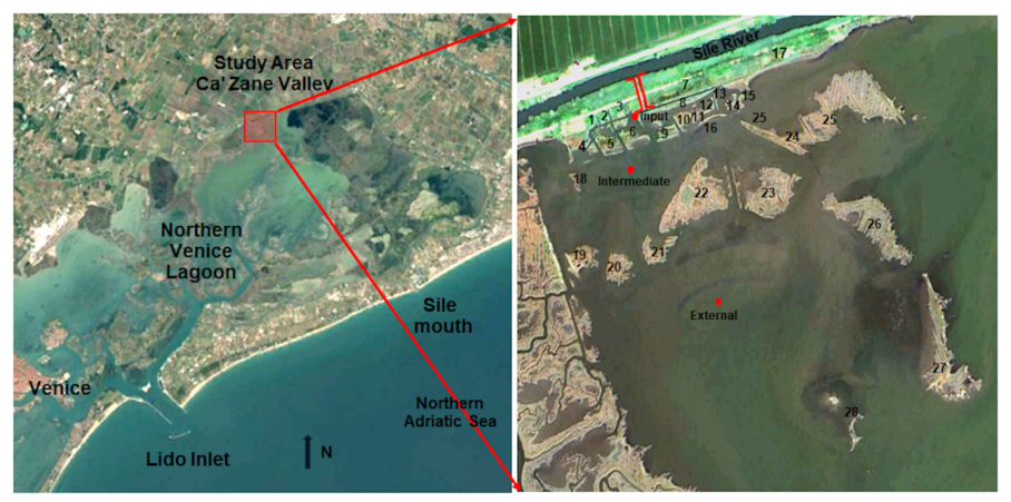
The freshwater diversion canal from the Sile River is in the innermost region of the northern lagoon basin in Ca’ Zane Valley. Before (October 2018) and after (monthly: from June 2020 to October 2021 and occasionally in subsequent periods) freshwater inputs, salinity values were measured at three stations (input station, intermediate station and external station, Figure 1) approx. 15 m in diameter.

2.2. Mapping of Halophytic Habitats

Prior to restoration, this area was predominantly characterized by halophytic vegetation typical of poly- to euhaline environments [10,11,12,13], although frequent flooding from the Sile River at the lagoon margin during particularly rainy conditions allowed the presence of species typical of intermediate salinity.

Halophytes are plant species adapted to grow in soils characterized by high salinity levels, with salt concentrations that may reach up to 20%, generating considerable osmotic stress. These physiological constraints select for specialized taxa capable of tolerating and regulating internal salt concentrations. Halophytic species form structured plant communities whose composition and spatial organization depend on several environmental drivers, including sediment texture, elevation, frequency and duration of tidal inundation, and the mean annual salinity of the interstitial waters saturating the substrate [14].

Because each species is characterized by a specific tolerance range within which its physiological performance and ecological fitness reach optimal conditions, the coexistence of multiple halophytic taxa occurs only when their tolerance thresholds partially overlap [15]. Consequently, even minor variations in hydrological or salinity regimes may lead to substantial shifts in species composition, vegetation zonation, and habitat structure.

The mapping of halophytic habitats was conducted by first establishing a baseline spatial framework of emergent salt marsh vegetation distribution in 2018 (pre-restoration conditions). This baseline was subsequently compared with the spatial configuration recorded in 2024 (post-restoration conditions), following the implementation of hydraulic–morphological interventions for freshwater diversion from the Sile River and the transplantation of reedbeds [16].

Field campaigns were conducted along the lagoon margin and the adjacent salt marshes for a total of 31 salt marsh platforms (S-MPs) located in proximity to the freshwater input (Figure 1). Repeated boat-based and ground-based surveys across the lagoon margins and adjacent salt marshes were carried out between April and October 2018 for the baseline pre-restoration mapping; the same approach was followed during the post-restoration mapping in October 2024. Where accessibility allowed, consolidated marshes were also surveyed on foot following linear transects. Vegetation surveys included the identification of dominant and accompanying species, the estimation of percentage cover, and the delineation of habitat boundaries using georeferencing, in-field data collection, UAV-assisted observations, and GIS-based mapping. Vegetation cover was estimated using visual Point Intercept/Step-Point [17] procedures adapted for salt marsh vegetation, while photographic documentation and UAV imagery were used to support the interpretation of vegetation mosaics and inaccessible areas.

This integrated field- and GIS-based approach allowed a quantitative comparison between pre- and post-restoration conditions and supported the evaluation of salinity-driven vegetation dynamics. Additional field validation surveys were subsequently performed to confirm polygon attribution and vegetation boundaries.

2.3. Field Campaigns and GIS Workflow

Following the acquisition and preprocessing of field survey data, the digital cartographic product was developed using the open-source GIS software QGIS (versions 2.18 “Las Palmas” and 3.0 “Girona”), integrated with GRASS GIS 7.4.4 [18].

Spatial analyses and georeferencing procedures were conducted in EPSG:32632 (WGS84/UTM zone 32N), while local cartographic layers originally provided in EPSG:3004 were reprojected within the QGIS environment.

In the initial phase, Landsat 8 OLI imagery (Collection 1 Tier 1, TOA Reflectance) collected from July to December 2017 was used as preliminary cartographic support to distinguish water-covered areas, emerged landforms, and salt marsh systems at low spatial resolution. Subsequently, Sentinel-2A orthoready Level-2A imagery acquired from April to October 2018 was used to refine shoreline delineation and marsh boundaries under mean tidal conditions, providing baseline polygons of the study area.

To further improve spatial resolution and increase the accuracy of vegetation boundary delineation, additional high-resolution orthophotos provided by Magistrato alle Acque (now ALV, Authority for the Venice Lagoon)—Consorzio Venezia Nuova (MAV-CVN), together with Veneto Region WMS/WMTS orthophotos from the 2018 regional aerial survey (with a spatial resolution of approximately 18 cm), were integrated within the GIS environment.

Data acquired during UAV field campaigns were additionally used to improve the interpretation of dense or poorly accessible vegetation assemblages, particularly reedbeds dominated by Phragmites australis located near the freshwater intervention embankment. UAV surveys were conducted following linear flight paths at an approximate 45–50 m altitude, allowing orthophoto generation with an estimated spatial resolution with an approximate 24 cm ground resolution.

Subsequent spatial processing involved the manual digitization and polygon delineation of raster datasets into vector layers. Vegetation polygons were delineated manually according to in-field observations, floristic composition, photographic documentation, and UAV-assisted interpretation derived from in situ surveys. In highly heterogeneous areas characterized by intermingled vegetation assemblages, polygons were classified as mixed vegetation mosaics according to the dominant co-occurring taxa rather than attempting species-level micro-segmentation. In S-MPs characterized by more complex vegetation assemblages, GPS-based perimeter acquisition (gpx tracks) was additionally performed during field surveys to improve polygon delineation accuracy.

Given that the cartographic representation included both a general overview map at a 1:10,000 scale and higher-detail patch-based interpretation of individual S-MPs, the effective minimum mappable unit (MMU) varied according to the mapping scale and local vegetation complexity. Very small or poorly distinguishable vegetation patches were not always represented individually in the general overview map; however, these patches were considered during detailed field interpretation and polygon delineation of individual S-MPs. Where vegetation assemblages formed highly fragmented patterns, polygons were attributed according to the dominant species composition or classified as mixed vegetation mosaics.

Finally, for each mapped polygon, geometric and vegetation-related attributes were calculated using QGIS geoprocessing tools. These included the total patch area and the estimated surface (m²) occupied by the dominant genus or, where taxonomic resolution allowed, by the dominant species. The resulting geodatabase provides a spatially explicit representation of vegetation distribution suitable for ecological assessment, habitat monitoring, and quantitative analysis of habitat extent.

2.4. Phragmites Australis Transplant Protocol

Phragmites australis was transplanted into the S-MPs using 15–20 cm sods collected along the banks of the Siloncello River, which flows into the lagoon a few kilometers from the restoration area. Sods were collected and transplanted by fishermen and hunters selected through a public tender from eroding riverbanks, where they would otherwise have naturally detached and fallen into the river bed during seasonal floods. The sods, collected in spring and autumn, were immediately transported to the transplant sites and embedded into the sediments of the S-MPs. Their establishment success was monitored every six months, increasing the number of transplants in the areas where the initial transplants proved successful.

2.5. Halophytic Cover Determination

Vegetation cover was quantified for each S-MP by subdividing the area into homogeneous sub-units based on species composition and cover; field-based cover estimations were integrated with polygon interpretation supported by UAV imagery and photographic documentation. Within each sub-area, vegetation cover was visually estimated using visual Point Intercept/Step-Point procedures adapted for salt marsh vegetation and phytosociological procedures [19,20].

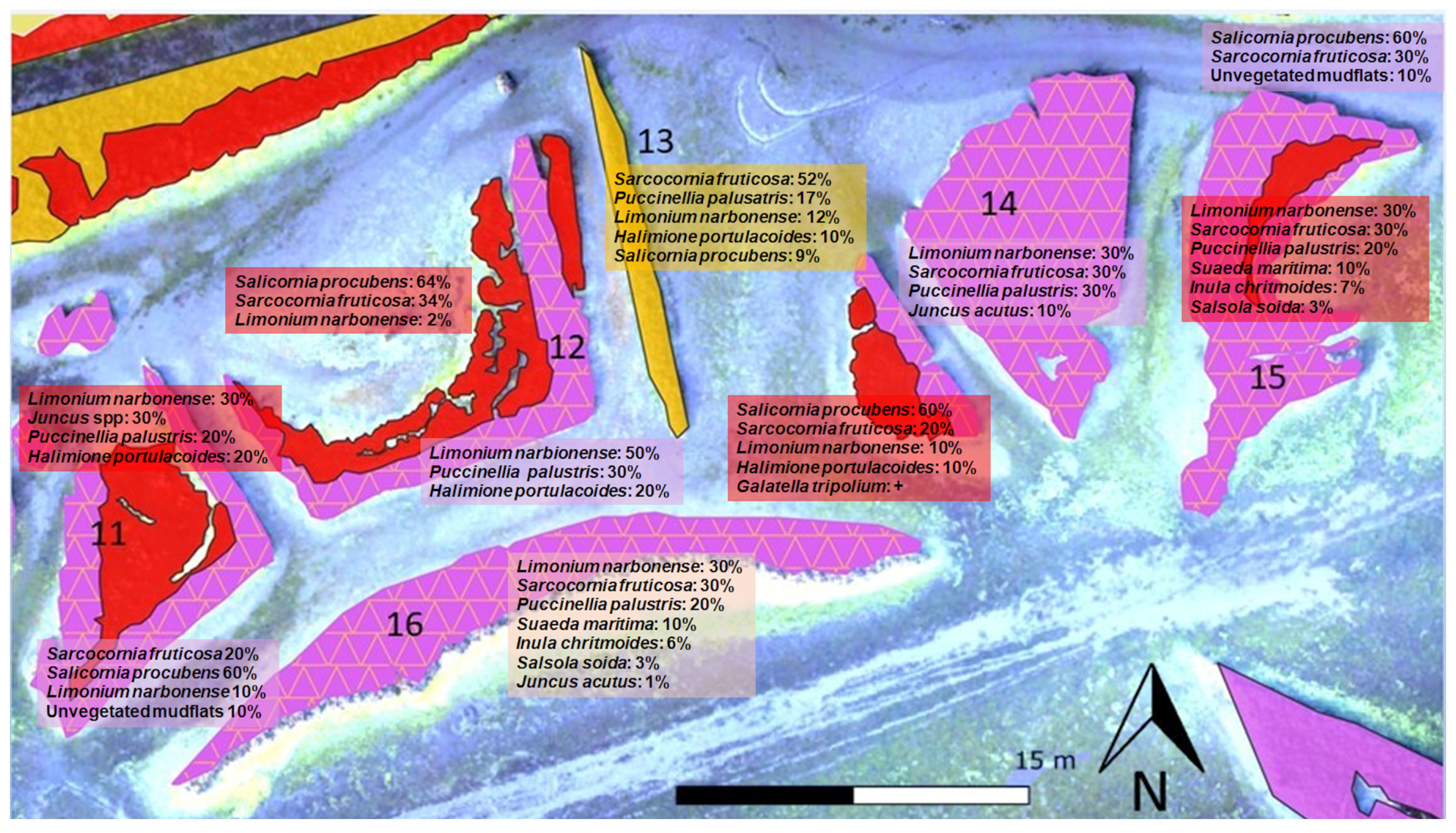
An example of vegetation mapping regarding salt marshes 11–16 in October 2018 is reported in Figure 2.

The overall vegetation cover for each S-MP was subsequently calculated by weighting the percentage cover values recorded in each sub-area according to its proportional surface area. Final cover percentages were therefore normalized to the total area of the respective S-MP, ensuring comparability among sites of different sizes and internal heterogeneity. Values were subsequently weighted according to polygon area; therefore, cumulative cover values did not exceed 100% at the S-MP scale.

For the analysis of temporal changes, data collected under baseline conditions (2018, pre-restoration) were compared with those obtained under final conditions (2024, post-restoration). The comparison focused on S-MPs 1–31. S-MPs 1–28, where measurable changes in vegetation composition and cover were observed, were analyzed together. S-MPs 29–31, where salinity levels remained consistently high and no significant vegetation changes occurred during the study period, were analyzed separately and considered as control S-MPs (blank).

In S-MPs 1–28 vegetation dynamics was assessed at two spatial scales: (1) global scale analysis, including all 28 S-MPs affected by the restoration measures, in order to evaluate the overall response of halophytic vegetation to freshwater diversion; (2) reduced analysis restricted to S-MPs 1–17, where salinity values following freshwater diversion decreased to values < 6 psu, allowing for a targeted assessment of vegetation shifts under markedly salinity-reduced conditions.

This dual analytical approach enabled the distinction between generalized vegetation trends across the intervention area and specific responses associated with substantial salinity decline, thereby improving the interpretation of ecological trajectories following hydraulic restoration.

2.6. Statistical Analyses

Vegetation data were analyzed to assess changes in plant community composition between 2018 (pre-intervention) and 2024 (post-intervention). The dataset consisted of species relative cover values (%) collected at the same S-MPs in both years, thus allowing a paired/repeated-measures design.

All statistical analyses were performed in R using the packages vegan, stats, and pairwise Adonis [21].

Species cover data (% relative cover) were arranged in a species-by-sample matrix and transformed using square-root ($y^{\prime }=\sqrt{y}$) transformation to reduce the influence of dominant taxa and improve the balance between common and rare species [22].

Community dissimilarity was calculated using the Bray–Curtis index [23] $(B{C}_{ij}=1-{\displaystyle \frac{2C_{ij}}{S_i+S_j}})$ where $C_{ij}$ is the sum of the shared abundances between samples $i$ and $j$ and $S_i$, $S_j$ are the total abundances in each sample. This index is widely used for ecological abundance and cover data because it is robust to zero inflation and ignores joint absences [22].

Differences in vegetation composition between 2018 and 2024 were tested using a paired PERMANOVA (Permutational Multivariate Analysis of Variance) implemented with the adonis2 function in the vegan package [21,24]. Statistical significance was assessed through permutation tests (999 permutations) [24].

To verify whether significant PERMANOVA results were due to differences in centroid location rather than differences in dispersion, a PERMDISP (Permutational Analysis of Multivariate Dispersions) analysis (betadisper) was also conducted following [25].

Changes in community diversity were evaluated using.

-

The Margalef species richness index (R = (S − 1)/ln N) [26];

-

The Shannon diversity index ($H^{\prime }=-{\sum }_{i=1}^S{p}_i\mathrm{l}\mathrm{n}{p}_i)$ [27];

-

The Simpson diversity index ($D=1-\sum p_i^2$) [28];

-

Pielou’s evenness (J = H’/ln S) [29].

Where S is the number of species, N is the number of individuals, and $p_i$ is the relative abundance of species $i$.

Species-specific temporal changes were assessed using paired non-parametric Wilcoxon signed-rank tests [30], followed by Benjamini–Hochberg False Discovery Rate (FDR) correction for multiple comparisons [31].

The magnitude of temporal compositional change at each S-MP was quantified using paired Bray–Curtis dissimilarity values, and differences among S-MPs groups were compared using Mann–Whitney U tests [32].

To identify species contributing most strongly to temporal changes, species-specific paired analyses were performed for each taxon.

In addition to the full set of S-MPs 1–28 located within the intervention area, two additional subsets were analyzed separately:

• S-MPs 1–17, representing the area expected to experience the strongest impact of the intervention due to a mean salinity < 6 psu;
• S-MPs 29–31 (control S-MPs), located outside the main impact area and expected to remain relatively stable over time.

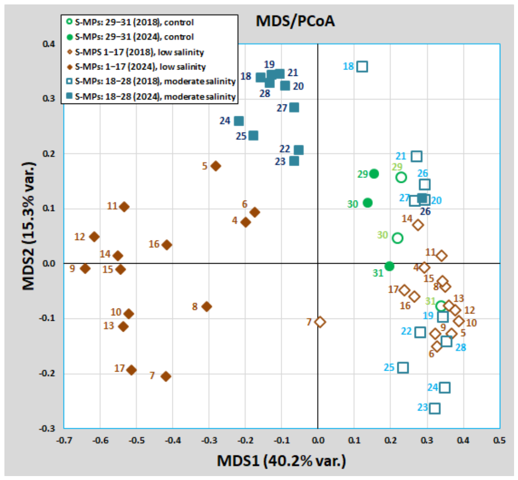
Finally, multidimensional scaling (MDS) was performed using Principal Coordinates Analysis (PCoA) based on a Bray–Curtis dissimilarity matrix calculated from square-root-transformed species cover data [23]. Analyses included all S-PMs and both sampling years (2018 and 2024). The first two ordination axes were used to visualize compositional differences among S-MPs and treatment groups.

3. Results

3.1. Venice Lagoon Surveys

Before freshwater diversion into the lagoon (May 2020), the upper area of the northern basin, namely the Ca’ Zane Valley, was not affected by freshwater inflow, except for occasional inundations from the Sile River during periods of intense rainfall. In this area, S-MPs (lagoon border and adjacent salt marshes) cover a total surface of 98,175 m² (9.82 ha). Salinity showed a relatively narrow gradient, with values ranging from 25–30 to 43 psu in the more confined areas and from 33–38 psu in zones characterized by higher water exchange.

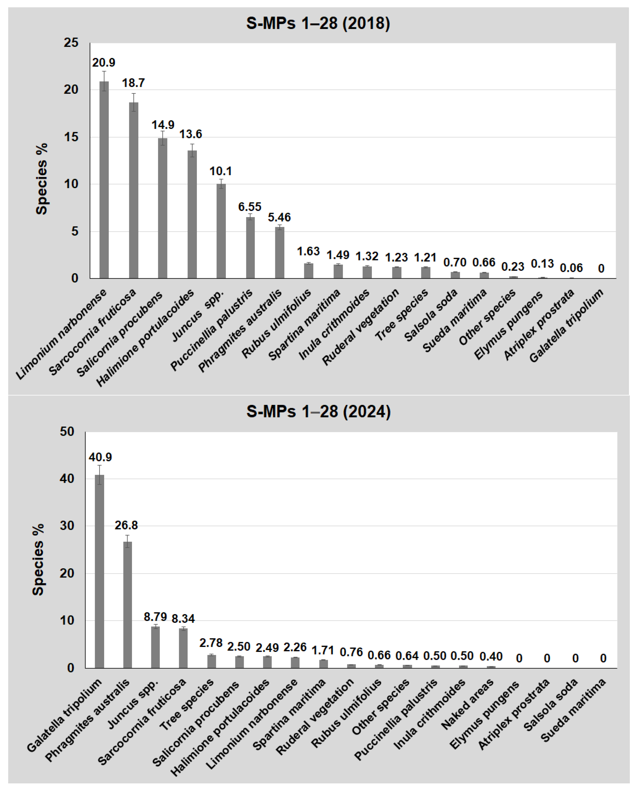
Under these salinity conditions, in October 2018 S-MPs 1–28 were mainly colonized by the halophytic species Limonium narbonense (20.9%), Sarcocornia fruticosa (18.7%), Salicornia procumbens subsp. veneta (14.9%), Halimione portulacoides (13.6%), and Juncus maritimus and J. acutus considered together (10.1%), followed by the other species shown in Figure 3. Phragmites australis colonized approximately 5.46% of the total area along the lagoon border (5363 m²) and was completely absent from the salt marshes.

These percentage covers of halophytic vegetation were calculated by weighting each S-MP according to its surface area (

Table 1. Surface of S-MPs 1–28.

S-MP	Surface	S-MP	Surface	S-MP	Surface	S-MP	Surface
	m2		m2		m2		m2
1	860	8	1917	15	407	22	11,355
2	760	9	1143	16	373	23	8948
3	1512	10	1105	17	1813	24	4415
4	2176	11	356	18	571	25	17,562
5	2168	12	417	19	2940	26	12,731
6	1687	13	75	20	3030	27	10,685
7	5512	14	474	21	2332	28	851
Total area 98,175 m2

), as derived from QGIS under mean water level conditions.

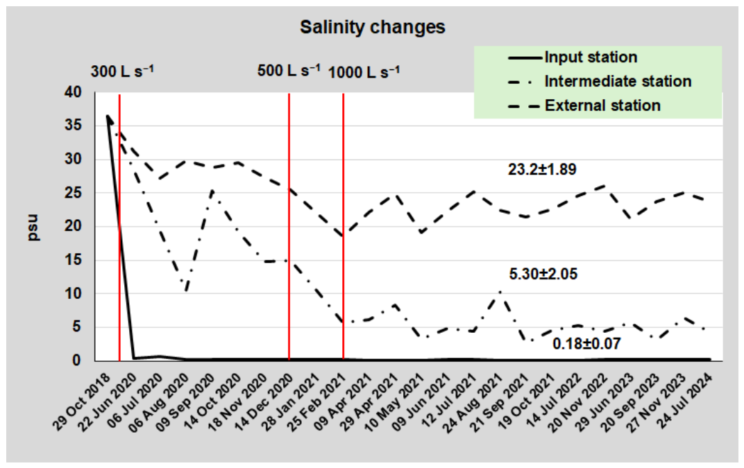
In May 2020, the introduction of approx. 300 L s⁻¹ of freshwater from the Sile River in the lagoon began. In December 2020, water input increased to 500 L s⁻¹, and from February 2021 to the present, freshwater input has been raised to approx. 1000 L s⁻¹. Salinity values before and during the three flow regimes (300, 500, and 1000 L s⁻¹) at the three monitoring stations (St. 1: input canal; St. 2: intermediate station; St. 3: external station) are shown in Figure 4.

Following the initiation of freshwater inputs in May 2020, salinity decreased significantly, and after February 2021, when freshwater input increased to approx. 1000 L s⁻¹, mean salinity values at stations 1, 2 and 3 were: 0.18 ± 0.07, 5.30 ± 2.05 and 23.2 ± 1.89 psu, respectively.

In some S-MPs more exposed to the reduction in water salinity, the salinity of the soil porewater was also verified, and in those where P. australis established and expanded, it was always less than 5 psu (usually 0.5–3.0 psu).

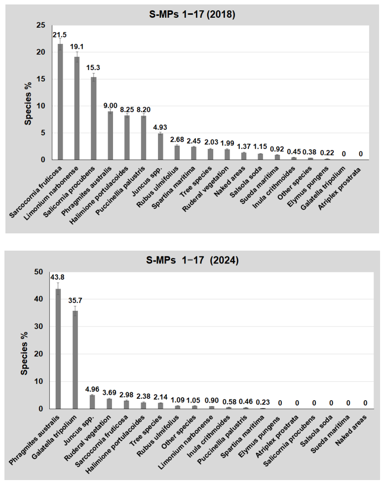
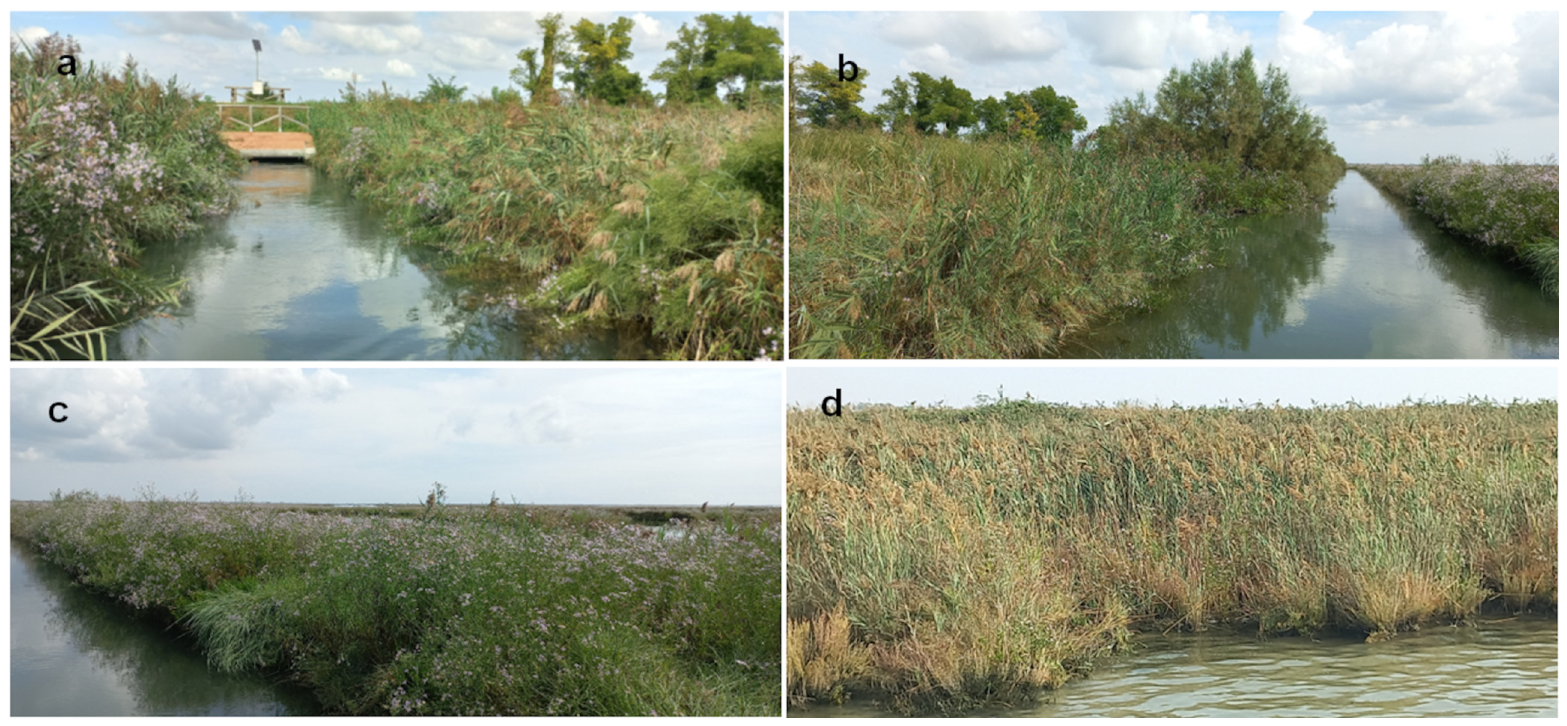
Consequently, vegetation dominance within total S-MPs changed markedly between 2018 and 2024 (Figure 3). The most evident change was the expansion of Galatella tripolium (Figure 3 and Figure 5), a species that was either absent or negligible in 2018. It was abundant only near the mouths of rivers such as the Dese and Siloncello, where salinity is naturally lower. In autumn 2024, after the salinity decrease, G. tripolium accounted for 40.9% (approx. 4.02 ha) of total vegetation cover in S-MPs 1–28 (approx. 9.82 ha), giving the salt marshes an intense blue coloration due to its 1–2 m high inflorescences, which overtopped most other species.

Simultaneously, Phragmites australis increased from 5.46% to 26.8%, colonizing mainly the areas closest to the freshwater inlet (Figure 4 and Figure 5). However, to promote its faster diffusion this species was transplanted in all the 28 S-MPs, and this favored its expansion especially in those characterized by a lower salinity (S-PMs 1–17).

In contrast, the percent cover of Limonium narbonense decreased from 20.9% to 2.26%, Sarcocornia fruticosa from 18.7% to 8.34%, Salicornia procumbens subsp. veneta from 14.9% to 2.50%, and Halimione portulacoides from 13.6% to 2.49%. The remaining species underwent less pronounced changes.

If we consider S-MPs 1–17, which after freshwater input were exposed to mean salinity values < 6 psu (Figure 6), the changes were even more pronounced, especially for P. australis, for which diffusion was enhanced by 5400 transplants of 15–20 cm plant sods.

In 2018, this area was dominated by Sarcocornia fruticosa (21.5%), Limonium narbonense (19.1%), and Salicornia procumbens subsp. veneta (15.3%). By autumn 2024, these species had been largely replaced by Phragmites australis (43.8%) and Galatella tripolium (35.7%), while the cover of all other species fell below 5% or became negligible.

Species such as Salicornia procumbens, Suaeda maritima, Elymus pungens, Salsola soda, and bare areas recorded in 2018 disappeared in 2024. Atriplex prostrata Boucher ex de Candolle subsp. latifolia was absent both before and after salinity changes.

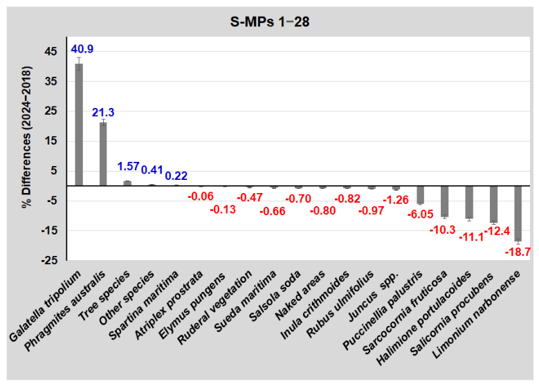
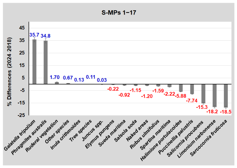
The extent of vegetation changes is highlighted by Figure 7, which shows the percent differences between surveys conducted in 2018 and 2024 in both S-MPs 1–28 and S-MPs 1–17 (salinity < 6 psu).

In S-MPs 1–28, G. tripolium and P. australis increased by 40.9% and 21.3%, respectively, together accounting for 62.2% of total vegetation cover. Conversely, significant decreases were observed for L. narbonense (−18.7%), S. procumbens (−12.4%), H. portulacoides (−11.1%), S. fruticosa (−10.3%), and P. palustris (−6.05%), while other species showed only negligible variations (<1.3%).

In S-MPs 1–17 (salinity < 6 psu), G. tripolium (+35.7%) and P. australis (+34.8%) together showed an overall increase of approx. 70%, with reed expansion progressively replacing halophytic communities. The species most negatively affected by salinity reduction were S. fruticosa (−18.5%) and L. narbonense (−18.2%), followed by S. procumbens (−15.3%), P. palustris (−7.74%), and H. portulacoides (−5.88%), whereas the remaining species exhibited only minor changes. Atriplex prostrata in S-PMs 1–17 was missing.

3.2. Statistical Analyses

The results of the statistical analyses are shown in

Table 2. Results of statistical analyses.

Analyses	Number of S-MPs	Test	Results	Ecological Significance
PERMANOVA paired	S-MPs 1–28	Bray–Curtis + sqrt transformation	F = 32.50; R2 = 0.376 p < 0.0001	Highly significant compositional change between 2018 and 2024
PERMDISP		Dispersion Analysis	n.s.	No significant difference in dispersal
Diversity—Richness		Wilcoxon paired	p < 0.01	Significant reduction in species number
Diversity—Shannon		Wilcoxon paired	p < 0.0001	Significant reduction in diversity
Diversity—Simpson		Wilcoxon paired	p < 0.0001	Significant reduction in diversity
Diversity—Evenness		Wilcoxon paired	p < 0.01	Community dominated by a few species
PERMDISP	S-MPs 1–17	Dispersion analysis	p = 0.752	No significant difference in dispersal
	S-MPs 18–28	Dispersion analysis	p = 0.544	No significant difference in dispersal
	S-MPs 29–31	Dispersion analysis	p = 0.145	No significant difference in dispersal
Comparison of change intensity	S-MPs 1–17 vs. S-MPs 18–28	Mann–Whitney	p = 0.017	The S-MPs1–17 showed a significantly stronger change
Control	S-MPs 29–31	Bray–Curtis paired	Mean distance = 0.145 p = 1.00	No significant change

.

The PERMANOVA analysis shows a highly significant difference in vegetation composition between 2018 and 2024 across S-MPs 1–28 (F = 32.5, R² = 0.376, p < 0.0001), with a strong temporal shift in vegetation structure following the diversion waters from the Sile River. Approximately 38% of the total variation was explained by the factor “Year”. In contrast, the PERMDISP analysis was not significant (p = 0.615), indicating that the observed differences were not due to changes in multivariate dispersion (i.e., variability among samples) but instead reflect a real species change in vegetation rather than increased heterogeneity.

All diversity metrics showed a consistent and significant decline from 2018 to 2024. Margalef species richness decreased significantly (p < 0.01), indicating a reduction in the number of species per station. The Shannon diversity index decreased strongly (p < 0.0001), reflecting both reduced richness and increased dominance. The Simpson diversity index also decreased significantly (p < 0.0001), confirming stronger dominance by a few species. Evenness significantly decreased (p < 0.01), indicating that species abundances became more unevenly distributed. Overall, the community in 2024 showed less diversity, was more simplified, and was dominated by a lower number of taxa than in 2018.

A clear spatial gradient of salinity/species pattern change was observed. S-MPs 1–17, S-MPs 18–28 and S-MPs 29–31 showed a decreasing mean Bray–Curtis dissimilarity ranging from 0.752 (high change) to 0.544 (moderate change) and 0.145 (no significant change). In contrast, S-MPs 29–31, which showed no statistically significant changes in community composition or diversity between 2018 and 2024, were considered the “control S-MPs”.

The plot of the multidimensional scaling by considering all S-MPs (1–31) and both sampling years, 2018 and 2024, is shown in Figure 8.

The variance explained from MDS1 and MDS2 was 40.2 and 15.3%, respectively. The ordination shows a clear separation between pre-intervention (2018 on the right side, empty markers) and post-intervention (2024 on the left side, full markers) communities, particularly in the low-salinity S-MPs. These 2024 S-MPs cluster clearly on the left side of the ordination space, while the corresponding 2018 S-MPs are predominantly positioned on the right side, indicating a strong directional change in vegetation composition following the intervention driven by salinity change and P. australis transplants.

In contrast, moderate S-MPs show a smaller displacement between years, suggesting a weaker but still detectable compositional change over time.

The control S-MPs remain closely grouped across years on the right side with a limited separation between 2018 and 2024, indicating relative temporal stability in the absence of strong intervention effects. It is interesting to note that S-MP 26 also shows minimal variations and could be considered as a control station.

Overall, the ordination suggests that vegetation change was spatially structured and proportional to the expected intensity of the intervention, with the strongest compositional shifts occurring in S-MPs 1–17 where the decrease in salinity was greatest.

4. Discussion

The ecology of halophytic and semi-halophytic plants, as well as selected tree and shrub species recorded in the lagoon margins and salt marshes (namely S-MPs), are summarized in

Table 3. Halophytic and semi-halophytic species of the Venice Lagoon S-MPs and their relationship with salinity.

Species	Life Form	Salinity Tolerance (psu)	Salinity Optimum	Preferential Marsh Zone	Indicator Meaning	Main References
Rubus ulmifolius Schott	Perennial shrub	<5	Very low	Terrestrial ecotone	Freshwater influence, stable soils	[33,34]
Populus alba Linnaeus	Tree	<5	Very low	Marsh margins/islands	Stable soils	[33,34]
Phragmites australis (Cav.) Trin. ex Steud	Perennial reed	<5–10	Very Low to Low	Ecotone	Freshwater input	[33,35]
Juncus acutus Linnaeus	Perennial rush	≤10	Very Low to Low	Ecotone	Moderate halophytism	[33,36]
Tamarix gallica Linnaeus	Shrub/small tree	5–15	Low	Upper marsh	Episodic salinity	[34,37]
Elymus pungens (Pers.) Melderis	Perennial rush	5–15	Low	Upper marsh	Competitive species	[33,36]
Juncus maritimus Lam.	Perennial rush	5–15	Low	High marsh	Low flooding	[33,36]
Limonium narbonense Mill.	Perennial rosette	5–20	Low to Moderate	High marsh	Marsh maturity, stability	[38,39]
Galatella tripolium (L.) Galasso, Bartolucci & Ardenghi	Perennial forb	10–25	Moderate	Mid-marsh	Transitional salinity	[33,40]
Atriplex prostrata Boucher ex DC subsp. latifolia	Annual/perennial forb	10–25	Moderate	Mid–high marsh	Nutrient-rich, moderately saline sediments	[34,41]
Inula crithmoides Linnaeus	Perennial succulent forb	10–30	Moderate	Mid-marsh	Moderate–high-salinity	[38,39]
Halimione portulacoides (L.) Aellen	Perennial shrub	10–30	Moderate	Mid-marsh	Intermediate stress	[37,38]
Puccinellia palustris (Seen.) Hayek	Perennial grass	10–30	Moderate	Low–mid-marsh	Seasonal flooding, moderate salinity	[33,38]
Spartina maritima (M.A. Curtis) Fernald	Perennial grass	15–35	Moderate to High	Low–mid-marsh	Sediment accretion	[37,38]
Sarcocornia fruticosa (L.) A.J. Scott	Perennial succulent	20–50	High	Low–mid-marsh	Woody perennial, stable saline surfaces	[37,38]
Suaeda maritima (L.) Dumort.	Annual succulent	25–50	High	Low marsh	Highly saline, unstable sediments	[37,38]
Salicornia procumbens Sm. subsp. veneta.	Annual succulent	30–60	High–Hypersaline	Pioneer/low marsh	Extreme salinity stress	[37,38,41]

.

For each taxon, the following attributes were considered: life form, salinity tolerance range and ecological optimum, preferential marsh zone (e.g., low marsh, middle marsh, high marsh, lagoon margins), indicator meaning, and main references. Taxa were grouped into four salinity tolerance classes (<5 psu, <5 to 15 psu, 5 to 30 psu and 15 to 60 psu) to facilitate ecological interpretation of vegetation shifts in relation to salinity gradients. In addition, the typical colonized marsh zones and corresponding ecological indicator meaning were provided.

-

Species of Very Low Salinity Tolerance (<5 psu)

Species with very low salinity tolerance are typically confined to stable soils along lagoon borders and marsh margins influenced by freshwater inputs. Populus alba L. [33,34] and the persistent shrub Rubus ulmifolius Schott [33,34] exhibit minimal tolerance to salinity and preferentially colonize consolidated substrates along the upper marsh and lagoon margins. In 2018, these species were present only at the lagoon margins in the upper marshes. In 2024, they underwent only negligible changes.

-

Species of Very Low to Low Salinity tolerance (<5 to 15 psu)

The shrub/small tree Tamarix gallica L. represents the largest woody species occurring along lagoon margins and tolerates salinity levels between approx. 3 and 15 psu [34,37]. It is commonly used as a natural marker delimiting low lagoon borders and islands, colonizing areas subject to freshwater inputs and episodic intermediate salinities. By 2024, it was responsible for doubling the tree cover, which also includes Populus alba and Robinia pseudoacacia.

Several perennial halophytes and shrubs tolerate low to moderate salinity.

Phragmites australis (Cav.) Trin. ex Steud., a perennial reed colonizing freshwater-influenced areas, shows a salinity tolerance of 5–10 psu [33,35]. However, ref. [42] reported optimal growth between 0 and 5 psu, with survival up to 15–22.5 psu.

Juncus acutus L. tolerates salinity ≤10 psu [33,36], while Juncus maritimus Lam. tolerates 5–15 psu [33,36]. Elymus pungens (Pers.) Melderis (syn. Agropyron pungens (Pers.) R. et S.) tolerates approx. 5–15 psu [33,36].

-

Species of Low to Moderate Salinity Tolerance (5 to 30 psu)

Limonium narbonense Mill. tolerates 5–20 psu [38,39]. Atriplex prostrata Boucher ex DC (syn. Atriplex latifolia Wahlenb) and Galatella tripolium (L.) Galasso, Bartolucci & Ardenghi (syn. Aster tripolium L.) show tolerance ranges of approx. 10–25 psu [33,37,39,40]. These species typically occupy the upper and middle marsh zones, where salinity fluctuations are moderate and inundation frequency is lower than in the pioneer low marsh.

Species adapted to moderate–high-salinity conditions dominate the middle and lower marsh zones: Inula crithmoides L. tolerates approx. 10–30 psu [38,39]; Halimione portulacoides (L.) Aellen [37,38] and Puccinellia palustris (Seen.) Hayek [33,38] tolerate similar salinity ranges.

-

Species of Moderate to Very High Salinity tolerance (15 to 60 psu)

The perennial grass Spartina maritima (Curtis) Fernald occurs within the 15–35 psu range [37,38].

Among the annual succulent plants, which display broad ecological amplitudes, Sarcocornia fruticosa (L.) A.J. Scott and Suaeda maritima (L.) Dumort [37,38] tolerate wide salinity intervals (20/25 psu to 50 psu):

The species with the widest salinity tolerance is Salicornia procumbens subsp. veneta (Pignatti & Lausi) Sciuto, M.A. Wolf, Sfriso, Brancaleoni, Iberite & Iamonico (syn. Salicornia veneta Pignatti & Lausi) [43], a pioneer taxon of the low marsh capable of colonizing high to hypersaline environments (30 to >60 psu) [37,38,41]. This species is typically associated with recently emerged or frequently inundated substrates characterized by strong evaporative concentration.

Overall, the vegetation recorded in the pre- and post-recovery intervention showed a clear ecological zonation along the salinity gradient, with species distribution reflecting physiological tolerance thresholds and hydrological regimes. Previous studies have demonstrated that halophytic species in the lagoon are associated with well-defined salinity and elevation ranges, and that their presence reflects the combined effects of flooding frequency, sediment characteristics, and soil salinity [44,45,46]. Such zonation patterns have been documented extensively within the Venice Lagoon salt marshes and are widely recognized as reliable ecological indicators of geomorphological and hydrodynamic processes (e.g., tidal regime influences species zonation from low to high marshes [44].

Historically, under conditions of high salinity, the most representative halophytic species in the study area included: Sarcocornia fruticosa (L.) A.J. Scott, Salicornia veneta Pignatti & Lausi, Halimione portulacoides (L.) Aellen, Suaeda maritima (L.) Dumort, Salsola soda L., Limonium narbonense Mill., Limonium serotinum Pignatti, Inula crithmoides L., Spartina spp., Juncus acutus L. and Juncus maritimus Lam [15]. The freshwater diversion implemented by the LIFE Lagoon Refresh project was therefore expected to modify these environmental drivers promoting shifts from poly–euhaline halophytic communities toward more mesohaline or oligohaline assemblages, with a consequent increase in habitat biodiversity and ecological functionality. Indeed, in the Venice Lagoon mesohaline and oligohaline habitats were markedly reduced by the diversion of the main rivers carried out since the 15th century [2]. As a result, the lagoon is currently strongly marinized, with a scarcity of salinity gradients and species that colonize the less salty areas.

Salinity represents the primary environmental filter in lagoon salt marshes, where ecological conditions are highly restrictive and variable. Consequently, vegetation diversity is typically limited to 10–15 specialized species only. In 2018, elevated salinity conditions favored species such as Sarcocornia fruticosa (optimum 20–50 psu) [37,38], Limonium narbonense (5–20 psu) [38,39], and Salicornia procumbens subsp. veneta (30–60 psu) [37,38,41].

In the pre-restoration survey (2018) these three species were dominant in both areas: S-MPs 1–28 (total surface area: 9.28 ha) and S-MPs 1–17 (total surface area: 2.28 ha). They accounted for 54.5% (approx. 5.35 ha) and 55.9% (approx. 1.28 ha) of the total plant cover, respectively.

In the post-restoration survey (2024) their cover decreased markedly, reaching 13.1% (approx. 1.28 ha) in S-MPs 1–28 and 3.88% (approx. 0.088 ha) in S-MPs 1–17.

Sarcocornia fruticosa (Habitat 1420, “Mediterranean and thermo-Atlantic salt marsh scrubs and grasslands—Sarcocornetea fruticosi”) accounted for 18.7% of S-PMs 1–28 in 2018 but decreased to 8.34% in 2024. This perennial succulent typically dominates slightly elevated zones where flooding frequency is reduced but porewater salinity remains persistently high. Under stable saline conditions, it often forms dense monospecific stands that influence sediment trapping and marsh accretion processes.

Limonium narbonense (Habitat 1510, “Salt steppes dominated by Limonium spp.”) in 2018 showed a cover of 20.9% in S-PMs 1–28 but declined dramatically to 2.26% in 2024, confirming its sensitivity to low-salinity regimes. Notably, although Habitat 1510 is reported as absent from the northern Adriatic Sea in the “Italian Manual for the Interpretation of Habitats” of Directive 92/43/EEC, [47] our findings suggest that its presence should be reconsidered and updated.

Salicornia procumbens subsp. veneta, together with Salicornia europaea and Salicornia patula (Habitat 1310, “Pioneer annual vegetation with Salicornia and other species of muddy and sandy zones”), dominated marginal low-marsh zones subject to frequent inundation and strong salinity fluctuations. In 2018, S. procumbens subsp. veneta in SPMs 1–28 formed monospecific populations at elevations of approx. 10–20 cm above mean tidal level, covering approx. 1.46 ha (14.9% of total vegetation). Following salinity reduction, its cover decreased to 0.25 ha (approx. 2.5% of total vegetation) in 2024, whereas it completely disappeared from S-MPs 1–17, where the mean salinity dropped below 6 psu (Figure 3 and Figure 7). This species is classified as a priority species under Annex II of the EU Habitats Directive, highlighting its high conservation value and the need for specific protection measures across European ecosystems. Nevertheless, within the wider lagoon system its distribution remains widespread and locally abundant across several salt marshes. Therefore, the loss of approx. 1.46 hectares can be considered ecologically marginal when compared with the overall extension and habitat heterogeneity of the lagoon. From a management and restoration perspective, this limited reduction represents an acceptable ecological trade-off if it contributes to the recovery and expansion of species such as P. australis. This reed species has experienced a marked regression over recent decades, mainly because of major hydrological modifications, including the historical diversion of rivers that significantly increased the average salinity of lagoon waters. Prior to these interventions, lower salinity conditions allowed extensive reed beds to develop across large portions of the lagoon landscape. Historically, these reed-dominated habitats played a fundamental ecological role by stabilizing sediments, improving nutrient cycling, enhancing water purification processes, and providing shelter, feeding grounds, and breeding sites for numerous bird, fish, and invertebrate species. Many of these associated species are now rare or locally declining within the lagoon ecosystem due to habitat loss and increasing salinization. Consequently, promoting the recolonization and spread of P. australis may contribute not only to habitat diversification but also to the restoration of important ecological functions and biodiversity values that characterized the lagoon before major anthropogenic alterations.

At lower salinities (<5–10 psu) in S-MPs 1–17, after water diversion and with the implementation of sod transplants, Phragmites australis exhibited a marked expansion (from 9.0% in 2018 to 43.8% in 2024), progressively replacing halophytic communities. This grass, which can exceed 3 m in height, spreads via robust rhizomes that eventually form dense monospecific populations, strongly reducing overall plant diversity. Further expansion is expected if low-salinity conditions persist.

Increasing the diffusion of Phragmites australis was a specific objective of the European project LIFE Lagoon Refresh (Life16 NAT/IT/000663), which aimed to restore the priority Habitat 1150* (Coastal Lagoon) by re-establishing a salt gradient through controlled freshwater inputs (300–1000 L s⁻¹). Historically widespread reed beds in the SCI 3250031 (Upper Venice Lagoon) had declined to approx. 34 ha [16]. Transplant of reed sods was carried out by amateur fishermen in all 28 S-MPs; however, successful establishment occurred mainly in S-MPs 1–17, where salinity decreased to near-optimal levels (mean value: 5.30 ± 2.05 psu, see St. 2), while more external S-MPs remained exposed to much higher salinities (mean value: 23.2 ± 1.89 psu see St. 3) with negligible plant survival. Therefore, after the first year, transplants continued mainly in S-MPs influenced by a suitable salinity. Reed expansion was due to both the growth of rhizomes and emission of new shoots, but in the following years the massive growth of diffuse new plants highlighted the importance of the natural diffusion via seeds produced both by the transplants and the plants already present along the lagoon margins.

Experimental studies [42] showed that P. australis had optimal growth at 0–5 psu, tolerated up to 15–22 psu for limited periods, and survived better when propagated from rhizomes rather than seedlings. Indeed, by investigating 27 natural reed habitats along the eastern and western coasts of Jutland, Denmark, these authors found that relative growth rates of rhizome-grown plants on a wet weight basis showed an optimum at 0–5 psu salinity but decreased at higher salinities. Phragmites australis adapted to saline conditions by adjusting the level of osmotically active solutes in its leaves. In the salinity range allowing survival (0–22 psu), osmolality in leaves of rhizome-grown plants was approx. 200 mmol kg⁻¹ higher than medium osmolality. In leaves of juvenile plants, osmotic pressure and chlorinity increased exponentially at salinity levels above 10 psu in the rooting medium, indicating a lower capability of osmoregulation. Die-back took place in the lower fringe of plants, before the onset of flowering, at sites where soil water salinities were higher than 15 psu within the rooting depth. In greenhouse experiments, juvenile plants produced from seeds and rhizome-grown plants, grown over a range of salinity levels, displayed different levels of salt tolerance. Both types of plants showed low mortality at salinity levels of 15 psu and lower. A total of 75% of the rhizome-grown plants survived 22.5 psu salinity in the rooting medium, whereas only 12% of the juvenile plants survived this salinity level. All plants died at increasing salinities. However, in our case, transplant stress likely limited establishment in higher-salinity marshes, although delayed colonization was observed 3–4 years later in some marshes.

No symptoms of reed die-back syndrome [48] were observed during field surveys in 2018. Interestingly, reed populations associated with nitrophilous ruderal species (e.g., Calystegia soldanella (L.) Roem. & Schult., Mentha aquatica L., Rubus ulmifolius and several Poaceae) appeared healthier than monospecific populations, supporting observations by [49] that mixed communities may enhance reed resilience, possibly due to substrate conditions that warrant further investigation.

The reduction in salinity also favored species adapted to intermediate or low-salinity conditions. At intermediate salinities, an unexpected massive increase in Galatella tripolium (optimum 10–25 psu [33,37] occurred, reaching 40.9% (4.02 ha) and 35.7% (0.81 ha) cover in S-MPs 1–28 and S-MPs 1–17, respectively. As a result, in autumn the salt marshes closest to the areas subject to a reduction in salinity turned into an intense blue color unlike anything ever seen before.

In the same areas, Juncus acutus and J. maritimus (Habitat 1410, “Mediterranean flooded grasslands—Juncetalia maritimi”) were also abundant. These species occurred in scattered and widespread patches in a great part of S-MPs 1–28, decreasing slightly from 10.1% (0.99 ha) in 2018 to 8.8% (0.86 ha) in 2024.

Spartina meadows (Habitat 1320, “Spartinion maritimae”), once very widespread in this area of the northern lagoon, were mostly confined to S-MPs 1, 6, 7 and 17 (approx. 1.49% of the total surface, i.e., 0.146 ha) in 2018. In 2024 S. maritima was also recorded in the most external S-PMs, 25 and, mostly, 27 and 28, but it decreased to 1.71% (0.168 ha).

Other species associated with intermediate salinities such as H. portulacoides, P. palustris, and I. crithmoides generally declined under reduced salinity conditions. H. portulacoides in SPMs 1–28 decreased from 13.6% to 2.49%, P. palustris from 6.55% to 0.50%, and I. crithmoides from 1.32% to 0.50%, whereas Elymus pungens, Atriplex prostrata, and Salsola soda, which in 2018 had a cover of 0.13, 0.06 and 0.70%, respectively, disappeared in 2024.

Ruderal herbaceous vegetation (Urtica dioica, Calystegia soldanella, Mentha aquatica, various Poaceae, and Rubus ulmifolius) exhibited moderate fluctuations, particularly in areas not yet colonized by reeds, whereas tree species (Populus alba, Robinia pseudoacacia, and Tamarix gallica) cover increased from 1.21% in 2018 to 2.78% in 2024.

5. Conclusions

The controlled reintroduction of freshwater from the Sile River into the northernmost area of the Venice Lagoon, combined with extensive transplants of P. australis, rapidly reshaped vegetation patterns, demonstrating that salinity reduction and transplants were the main drivers of taxa distribution. Within four years, the restoration of a salinity gradient with the diversion of 300–1000 L s⁻¹ from the Sile River transformed a predominantly poly–euhaline system (18–>40 psu) into a brackish environment, inducing predictable changes in vegetation according to species salinity tolerance.

Species characteristic of high–moderate salinity conditions such as Sarcocornia fruticosa, Salicornia procumbens subsp. veneta, Halimione portulacoides, and Limonium narbonense decreased markedly, especially below 6 psu (S-MPs 1–17). In contrast, moderate- to low-salinity species expanded significantly. G. tripolium became the dominant herbaceous species throughout the study area, while P. australis strongly increased, particularly in the lowest-salinity marshes, due to both low-salinity conditions and transplants. This rapid expansion of reedbeds (cover: 26.8% in S-MPs 1–28; 43.8% in S-MPs 1–17) highlights the recovery potential of P. australis under suitable salinity conditions, while the decline in hypersaline specialists reflects the trade-off inherent in salinity management, with local reductions in habitats adapted to extreme salinity. Nevertheless, considering the historical loss of freshwater inputs and reedbeds caused by lagoon marinization, the intervention partially restored the lagoon’s former ecological heterogeneity.

Beyond the ecological benefits observed at the local scale, the restoration of salinity gradients contributes to the long-term sustainability of coastal lagoon ecosystems by enhancing habitat diversity, ecological resilience, biodiversity conservation, and ecosystem services. These outcomes support the objectives of the European Green Deal, the EU Habitats Directive, and sustainable management strategies for transitional waters facing increasing environmental pressures related to climate change and human activities.