Diagnosing the Spatial Pattern, System Coupling Coordination, and Dominant Obstacles of Ecological Resilience Based on the RAR Framework: Evidence from Heilongjiang Province

Abstract

Enhancing ecological resilience is essential for safeguarding ecological security in high-latitude cold regions under the combined pressures of climate change and intensive human disturbance. Focusing on Heilongjiang Province, China, this study develops a multi-scale analytical framework based on the resistance-adaptability-recovery (RAR) perspective and covering 11 indicators to reveal the spatial differentiation, internal coordination, and dominant constraints of ecological resilience (ER). Quantifications were conducted using 2024 multi-source spatial data at a 1 km × 1 km grid scale, with results aggregated to 120 counties at the county scale and further identified by applying Global Moran’s I, hot spot analysis, the coupling coordination degree model, and the obstacle degree model. The results reveal spatial heterogeneity in ER and its components. Resistance is generally weak, adaptability is strong, and recovery is polarized. ER components exhibit positive spatial autocorrelation. Medium coordination predominates (47.5% of counties), followed by low coordination (33.33%) and high coordination (19.17%). Low-coordination is constrained by weak resistance and recovery. Identifying soil conservation and habitat quality as primary constraints, which jointly constrain 88.4% of counties. These findings provide a mechanism-oriented basis for differentiated ecological governance in cold-region ecological security barriers.

1. Introduction

Ecosystems are increasingly exposed to the combined pressures of global climate change and intensive human disturbances [1,2]. Against this background, enhancing ecological resilience, the capacity of ecosystems to absorb shocks, adapt to change, and recover from disturbance, has become a central concern in sustainable spatial governance [3,4]. Current research has not only deepened the understanding of the essence of resilience theory but has also made significant progress in operational assessment, multi-scale governance, and the dynamic evolution of coupled social-ecological systems (SES) [5,6]. The research paradigm is experiencing a profound shift from descriptive monitoring to dynamic simulation, from single-discipline analysis to interdisciplinary integration, and from qualitative metaphors to quantitative prediction [3,7,8]. Among the existing conceptual frameworks, the resistance-adaptability-recovery (RAR) framework has been widely adopted to characterize the multidimensional nature of ecological resilience [9,10,11,12,13]. In this framework, resistance reflects the basic capacity of ecosystems to withstand disturbances, adaptability refers to the ability to adjust structure and function under changing conditions, and recovery denotes the potential to regenerate after disturbance. Together, these three dimensions provide an effective basis for understanding resilience as a dynamic and internally differentiated property rather than a static ecological state [14,15,16].

However, existing studies often apply the RAR framework mainly to construct a composite resilience index, thereby reducing ecological resilience to a single overall score [17,18,19]. Although such an approach is useful for comparing general resilience levels, it pays insufficient attention to the interactions among resistance, adaptability, and recovery [20]. In practice, these three dimensions do not necessarily evolve synchronously. A region with relatively strong adaptability may still be constrained by weak resistance or poor recovery, and a seemingly high resilience score may therefore conceal internal imbalance or structural vulnerability [21]. This issue is especially important for ecological governance because the improvement of resilience depends not only on the overall level of resilience but also on whether its internal dimensions develop in a coordinated way [22]. Therefore, moving beyond simple composite assessment toward a mechanism-oriented diagnosis of internal coordination and dominant constraints has become a key task in ecological resilience research [23]. Our study tries to transcend the prevailing composite-index paradigm by introducing an integrated Assessment-Coordination-Diagnosis framework that reveals the internal structure of ecological resilience.

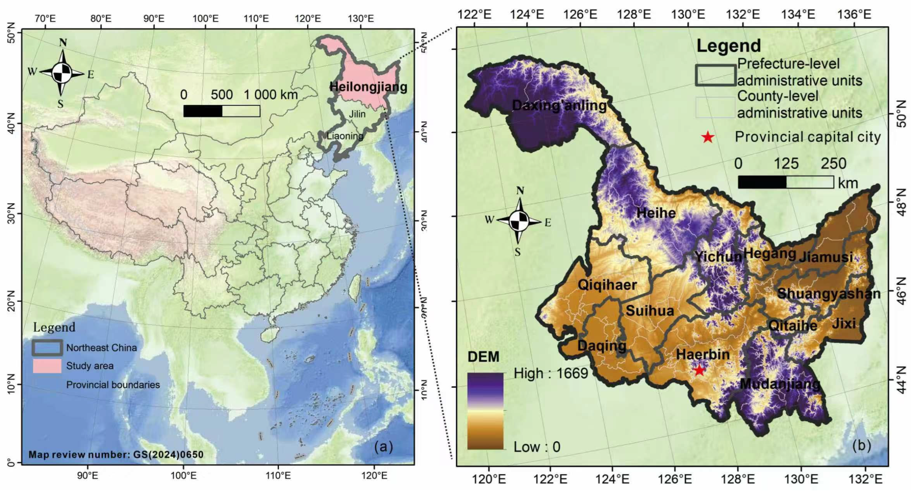
Heilongjiang Province provides a highly representative setting for such an investigation [24,25]. Located in the high-latitude frontier of Northeast China, it is a core component of China’s northern ecological security barrier and plays an important role in forest carbon sequestration, biodiversity conservation, water conservation, and regional climate regulation [26]. The Greater and Lesser Khingan Mountains, extensive wetlands, and forested landscapes in northern and eastern Heilongjiang constitute important ecological strongholds. At the same time, the province also contains vast black-soil plains and intensive agricultural production areas, especially in the west and southwest, where human disturbance, cultivated-land use pressure, and ecological vulnerability are comparatively stronger [27,28]. This coexistence of ecological strongholds and highly utilized production spaces makes Heilongjiang a region with pronounced spatial heterogeneity and clear contrasts in ecological background, landscape structure, and development intensity. Such characteristics make it particularly suitable for examining not only the spatial differentiation of ecological resilience but also the coordinated relationships and bottleneck constraints among its internal dimensions. The joint application of the coupling coordination degree model and the obstacle degree model with multi-scale (grid–county) zonal statistics, enabling identification of where, how coordinated, and why constrained systematically.

In this context, county-level analysis is especially meaningful. Counties are important units linking regional ecological governance, land-use management, and local development decision-making. Compared with broad provincial summaries, county-scale diagnosis is better able to reveal the spatial clustering of resilience, identify regional cold spots and hot spots, and provide a more direct basis for differentiated policy intervention. At the same time, resilience processes are inherently spatially heterogeneous within counties, and fine-resolution grid data are needed to capture local ecological variation before meaningful aggregation can be made. Research on two levels not only ensures the precision of data analysis but also facilitates the management of service ecosystems. Therefore, combining grid-level assessment with county-level diagnosis provides a useful way to connect ecological detail with governance relevance.

Against this background, this study seeks to address three key scientific questions in the context of the high-latitude cold region: (1) How are ecological resilience and its three internal dimensions (resistance, adaptability, and recovery) spatially differentiated across Heilongjiang Province at the grid and county scales? (2) To what extent do the three dimensions develop in a coordinated manner, and what spatial patterns do their coordination states exhibit? (3) Which sub-indicators act as the dominant constraints on county-level ecological resilience, and how do these constraints differ across counties with different coordination states? To address these issues, this study develops a multi-scale analytical framework for ecological resilience assessment in Heilongjiang Province. Accordingly, three specific objectives are pursued: to quantify resistance, adaptability, and recovery using multi-source spatial data and reveal their spatial heterogeneity; to evaluate the internal coordination state among the three dimensions through the coupling coordination degree model; and to diagnose the dominant obstacle factors restricting county-level ecological resilience under different coordination types. We further hypothesize that ER and its components exhibit significant positive spatial autocorrelation, the three dimensions are not synchronously developed, the dominant constraints are heterogeneous across counties, and the obstacle structure shifts systematically as counties progress from low to high coordination. This study aims to move from descriptive resilience assessment toward a more mechanism-oriented understanding of county-level ecological resilience and to provide empirical support for differentiated ecological governance in high-latitude cold-region provinces.

2. Study Area and Data

2.1. Study Area

Heilongjiang Province (43°26′–53°33′ N, 121°11′–135°05′ E) is situated in the northernmost and easternmost frontier of China (Figure 1). Characterized by a typical cold temperate continental monsoon climate, the province experiences long, harsh winters and short summers, rendering its natural ecosystems highly sensitive to climatic variations and slow to regenerate. Topographically and ecologically, it exhibits a diverse and foundational landscape: the Greater and Lesser Khingan Mountains in the north serve as crucial national ecological barriers with immense forest carbon sinks, while the Sanjiang and Songnen Plains form critical agricultural and wetland ecotones. This unique geographical endowment provides the region with a substantial baseline of ecological resistance but also imposes strict conservation constraints on large-scale developmental interventions. As a high-latitude cold region characterized by long winters, slow ecological succession, and strong sensitivity to disturbance, it serves as a representative case for understanding resilience mechanisms in other regions facing similar pressures.

The study encompasses all 120 county-level units in Heilongjiang Province. Socio-economically, Heilongjiang represents a classic old industrial base and resource-dependent province currently undergoing a profound and painful structural transition. Influenced by the depletion of coal and oil resources, alongside massive population out-migration, the province has become the most concentrated area of shrinking cities in China. Furthermore, the region exhibits extreme internal spatial heterogeneity. The central Harbin metropolitan area demonstrates polarized urban growth and economic concentration; the eastern coal-electricity-chemical bases face severe urban shrinkage and rigid industrial structures; and the western oil–chemical regions grapple with fragile saline–alkali environments. Therefore, in order to achieve sustainable revitalization of Heilongjiang Province, it is necessary to conduct an in-depth diagnosis of its spatial misallocation and internal coordination issues. These ecological, topographical, and socio-economic characteristics make Heilongjiang not only ecologically representative but also methodologically suitable for diagnosing internal resilience structures, rather than merely measuring their composite intensity.

2.2. Data Sources and Preprocessing

This study compiled a multi-source, high-resolution geospatial database to comprehensively evaluate urban ecological resilience. To ensure spatial consistency across heterogeneous data sources and to match the analytical grid scale, all raster datasets were uniformly reprojected to the WGS 1984 Albers Equal Area Conic coordinate system and resampled to a 1 km spatial resolution.

Specifically, as shown in

Table 1. Source of the multi-source datasets.

Datasets	Time	Data Source	Resolution
Land use	2024	China Land Cover Dataset (CLCD) (https://doi.org/10.5281/zenodo.18180184, accessed on 4 December 2025.)	30 m
NDVI	2024	NASA (https://www.earthdata.nasa.gov/, accessed on 4 December 2025)	500 m
DEM	2024	Copernicus DEM (https://panda.copernicus.eu/panda, accessed on 4 December 2025.)	500 m
Precipitation and potential evapotranspiration	2024	National Tibetan Plateau Data Center (https://www.tpdc.ac.cn/, accessed on 10 December 2025.)	1 km
Grain yield	2024	China City Statistical Yearbook	—
Road data	2024	OpenStreetMap (https://www.openstreetmap.org/#map=4/36.96/104.17, accessed on 10 December 2025.)	—

, land-use data were derived from the China Land Cover Dataset at a 30 m resolution, which provides annual 30 m land-cover maps for China. In this study, the CLCD data for 2024 were used to characterize the land-use structure of Heilongjiang Province and to support the calculation of ecosystem-service and landscape-pattern indicators. The CLCD classification system includes nine major land-use/land-cover categories: cropland, forest, shrubland, grassland, water, snow/ice, barren land, impervious surface, and wetland. The natural ecological baseline and topographic constraints were supported by the Normalized Difference Vegetation Index (NDVI) from NASA Earthdata, digital elevation models (DEM) from Copernicus, and meteorological data from the National Tibetan Plateau Data Center. Road networks were derived from OpenStreetMap. Finally, official statistical data—including grain yield extracted from the China City Statistical Yearbook—were collected to quantify specific resilience dimensions (e.g., food provision) and to cross-validate the reliability of the remote sensing and internet-derived datasets. During the grid-to-county scale transformation, these high-resolution raster metrics were aggregated to administrative units using zonal statistics.

3. Methodology

3.1. Study Process

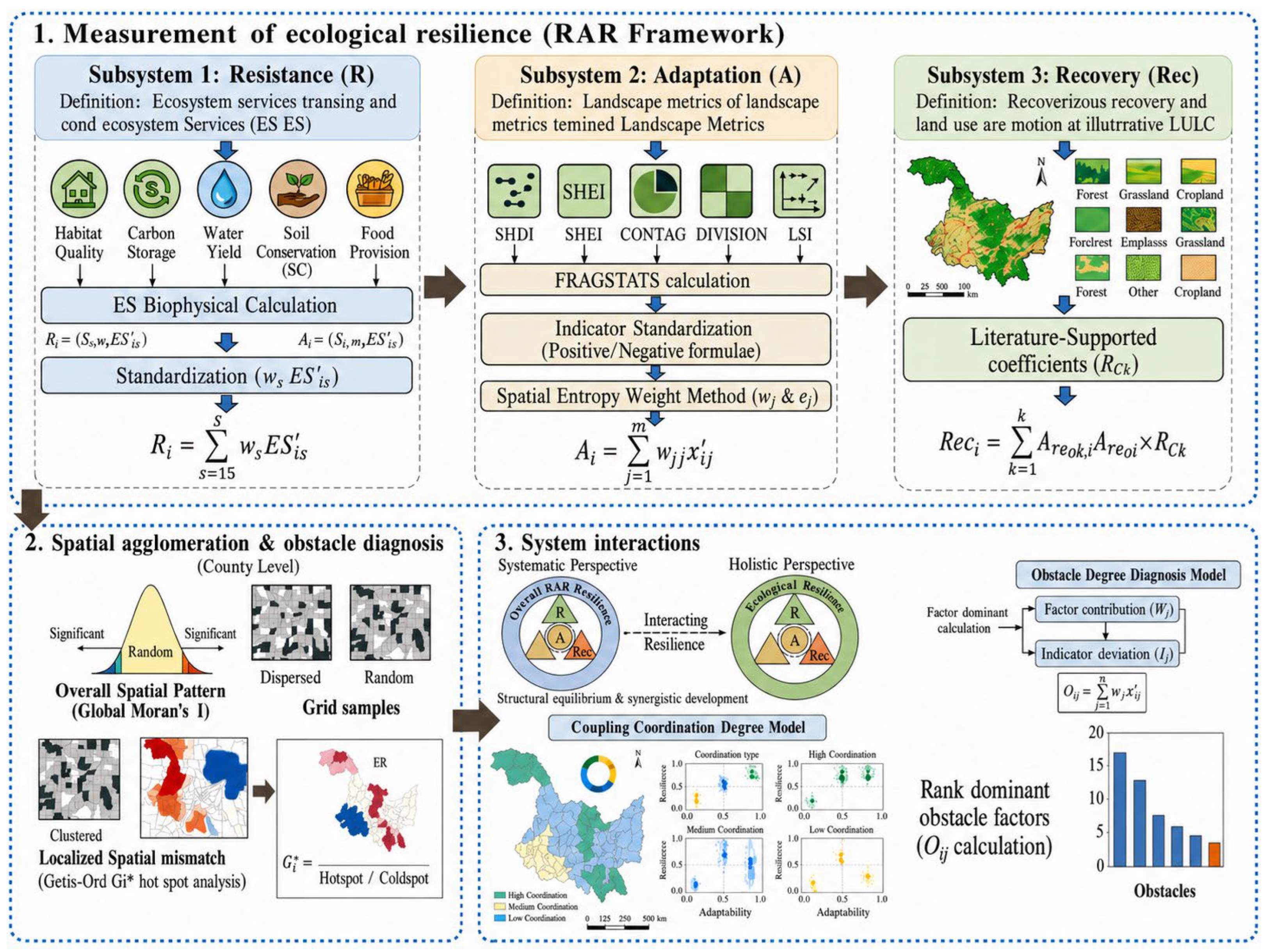
As illustrated in Figure 2, this study follows a structured analytical process primarily divided into three sequential stages.

Initially, a multi-scale analytical framework for ecological resilience assessment was operationalized through multidimensional indicators. Using multi-source spatial data at a 1 km × 1 km grid scale, we quantify resistance, adaptability, and recovery and identify their spatial patterns, as well as the overall ecological resilience pattern. Resistance was quantified by aggregating five key ecosystem services (habitat quality, carbon storage, water yield, soil conservation, and food provision) using the InVEST model and spatial allocation methods. Adaptability was evaluated through landscape metrics (SHDI, SHEI, CONTAG, DIVISION, and LSI) with weights determined by the spatial entropy method, while recovery was measured via area-weighted coefficients assigned to different land-use types.

Subsequently, grid-level results were aggregated to the county scale through area-weighted zonal statistics to identify regional spatial clustering using Global Moran’s I and Getis-Ord $G_i^{*}$ hot spot analysis. To mitigate the mismatch between administrative units and ecological boundaries, this study adopts a nested grid-to-county strategy. Grid scale preserves the intra-county heterogeneity to support sub-county interpretation. The county is retained as the diagnostic scale because it is the operational unit for ecological governance and land-use planning in China.

Third, the Coupling Coordination Degree Model (CCDM) was employed to evaluate the structural synergy among the RAR components, followed by the application of an obstacle degree model to diagnose the dominant limiting factors for each county. This process enables a transition from descriptive assessment to mechanism-oriented governance strategies for high-latitude cold regions.

3.2. Measurement of Ecological Resilience

Ecological resilience refers to the capacity of an ecosystem to absorb external natural or anthropogenic disturbances while maintaining its essential structure, functions, and identity, as well as its ability to reorganize and evolve. To comprehensively and spatially quantify this complex property, this study constructs a multi-dimensional evaluation framework based on the resistance-adaptability-recovery (RAR) model. The RAR framework logically decomposes ecological resilience into three sequential and interacting capacities: the inherent strength to withstand initial impacts (resistance), the structural flexibility to buffer and adjust to changes through spatial configuration (adaptability), and the capability to bounce back to a stable equilibrium state post-disturbance (recovery). Ecological resilience is characterized through these three perspectives.

3.2.1. Resistance

Resistance characterizes the fundamental defense mechanism of the ecosystem, reflecting its intrinsic ability to resist structural degradation and functional loss when facing external shocks. A robust provision of ecosystem services typically underpins a high level of ecological resistance. Ecosystem-service supply is not identical to resistance in the strict ecological sense, but treat it as a measurable proxy that captures the system’s current functional integrity. In this study, resistance is quantified by assessing five critical ecosystem services that represent the foundational ecological baseline of the study area: habitat quality, carbon storage, water yield, soil retention, and food provision. The spatial quantification of the five ecosystem services, which constitute the resistance dimension, is primarily executed using the Integrated Valuation of Ecosystem Services and Tradeoffs (InVEST) model and spatial allocation methods at a 1 km grid resolution [29].

• Habitat Quality

Habitat quality is calculated using the InVEST Habitat Quality module, which evaluates the status of biodiversity by assessing LULC types and the extent of anthropogenic threats [30].

$$Q_{xj}=H_j\left(1-\left({\displaystyle \frac{D_{xj}^z}{D_{xj}^z+k^z}}\right)\right)$$

(1)

where $Q_{xj}$ is the habitat quality of grid x with LULC type j; $H_j$ is the habitat suitability of LULC j; $D_{xj}$ is the total threat level; z is a scaling constant (default as 2.5); and k is the half-saturation constant.

2.

Carbon Storage

Carbon storage is estimated using the InVEST Carbon Storage module by aggregating four carbon pools for each LULC type: aboveground biomass ($C_{above}$), belowground biomass ($C_{below}$), soil organic matter ($C_{soil}$), and dead organic matter ($C_{dead}$) [31].

$$C_{total}=C_{above}+C_{below}+C_{soil}+C_{dead}$$

(2)

3.

Water Yield

Water yield is evaluated based on the Budyko curve and annual average precipitation using the InVEST Water Yield module [32].

$$Y_{xj}=\left(1-{\displaystyle \frac{AE{T}_{xj}}{P_x}}\right)\times P_x$$

(3)

where $Y_{xj}$ is the annual water yield for grid $x$ with LULC $j$; $AE{T}_{xj}$ is the actual evapotranspiration; and $P_x$ is the annual precipitation on grid $x$.

4.

Soil Conservation (SC)

Soil conservation is an essential regulating service that reflects the capacity of ecosystems to prevent soil erosion and retain sediment, thereby reducing land degradation and mitigating flood risks [33,34]. In this study, soil conservation was estimated as the annual difference between potential soil erosion and actual soil erosion using the following equations:

$$S{C}_x={RKLS}_x-{USLE}_x$$

(4)

$${RKLS}_x=R_x\times K_x\times L{S}_x$$

(5)

$$USL{E}_x=R_x\times K_x\times L{S}_x\times P_x\times C_x$$

(6)

where SCx denotes annual soil retention (t/hm²); RKLSx denotes the potential maximum soil erosion in the absence of vegetation and conservation measures (t/hm²); USLE denotes the actual soil erosion under existing land cover and management practices (t/hm²); Rx denotes the rainfall erosivity factor (MJ·mm/hm²·h); Kx denotes the soil erodibility factor (t·h/MJ·mm); LSx denotes the slope length-gradient factor; Cx denotes the vegetation cover and management factor; and Px denotes the support practice factor.

5.

Food Provision

As agricultural statistics are typically recorded at administrative levels, a spatial allocation method was employed to distribute the county-level grain yield to the 1 km grid scale. First, the total grain yield of each county was obtained from the China City Statistical Yearbook and matched to the corresponding county-level administrative unit. Second, cropland and pasture pixels identified from the CLCD were used as the spatial allocation mask because food provision is primarily generated from agricultural production spaces. Third, NDVI was used as the allocation weight to represent the relative spatial differences in vegetation growth conditions and potential agricultural productivity within each county [35]. The food provision assigned to each 1 km grid was calculated as follows:

$$F{P}_i={\displaystyle \frac{NDV{I}_i}{{\sum }_{i=1}^{n}NDV{I}_i}}\times Foo{d}_{county}$$

(7)

where $F{P}_i$ is the food provision allocated to grid $i$; $NDV{I}_i$ is the vegetation index value of grid $i$; and $Foo{d}_{county}$ is the total statistical food production of the corresponding county.

To assess the reliability of the ecosystem-service estimates, this study adopted a multi-source validation and consistency-check strategy. For food provision, the gridded results were checked through mass-balance consistency to ensure that the sum of 1 km grid values within each county was consistent with the original county-level grain-yield statistics. The spatial plausibility of food provision was further examined based on its correspondence with cropland distribution and NDVI. For habitat quality, carbon storage, water yield, and soil conservation, the simulated patterns were evaluated by comparing them with relevant ecological gradients and ancillary datasets, including land-cover composition, forest and wetland distribution, NDVI, precipitation, topography, and previously reported ecological patterns in Northeast China.

After calculating the biophysical quantities of these five ecosystem services, the values are standardized to eliminate dimensional differences. The comprehensive resistance capacity of each spatial unit is then computed by aggregating these standardized values. The calculation is as follows:

$$R_i={\displaystyle \sum _{s=1}^5}{w}_s{{ES}^{\prime }}_{is}$$

(8)

where $R_i$ represents the comprehensive resistance score of grid i; ${{ES}^{\prime }}_{is}$ is the standardized value of the s-th ecosystem service at grid i; and $w_s$ is the weight assigned to the corresponding ecosystem service.

3.2.2. Adaptability

Adaptability denotes the ecosystem’s capacity to mitigate potential damages and maintain structural stability through optimal spatial configuration [36]. This dimension is deeply related to the heterogeneity and connectivity of the landscape pattern. According to the theory of landscape ecology, this study measures the spatial configuration and adaptability of regional ecosystems through five core dimensions: diversity, evenness, aggregation/connectivity, degree of fragmentation, and morphological complexity [37,38]. Based on this, five assessment indicators with good balance and low redundancy were selected. Landscape spatial diversity and evenness are captured by the Shannon’s Diversity Index (SHDI) and Shannon’s Evenness Index (SHEI) [39], which respectively quantify patch-type richness and the relative dominance among patch types, jointly reflecting the variety of ecological niches available for adaptive reorganization. Connectivity and fragmentation are characterized by the Contagion Index (CONTAG) and the Landscape Division Index (DIVISION), where CONTAG measures the aggregation and contiguous distribution of dominant patches, directly indicating the landscape’s capacity to support species movement and ecological-process continuity. DIVISION quantifies the degree to which the landscape is subdivided, reflecting fragmentation-induced constraints on adaptive functioning [40]. Finally, the Landscape Shape Index (LSI) captures the geometric complexity and edge irregularity of patches, representing edge-effect intensity and structural elaboration of the landscape mosaic [41]. The five selected landscape metrics are calculated based on the FRAGSTATS 4.2 algorithms. The mathematical formulas and descriptions are as follows:

• Landscape spatial diversity (SHDI and SHEI)

$$SHDI=-{\displaystyle \sum _{i=1}^m}(P_i\mathit{ln}{P}_i)$$

(9)

$$SHEI={\displaystyle \frac{-{\sum }_{i=1}^m(P_i\mathit{ln}{P}_i)}{\mathit{ln}m}}$$

(10)

where m is the total number of patch types (land use categories), and $P_i$ is the proportion of the landscape occupied by patch type i.

2.

Connectivity and fragmentation (CONTAG and DIVISION)

$$CONTAG=\left[1+{\displaystyle \frac{{\sum }_{i=1}^m{\sum }_{k=1}^m\left[P_i\left(\frac{g_{ik}}{{\sum }_{k=1}^m{g}_{ik}}\right)\right]\ln \left[P_i\left(\frac{g_{ik}}{{\sum }_{k=1}^m{g}_{ik}}\right)\right]}{2\ln m}}\right]\times 100$$

(11)

$$DIVISION=\left(1-{{\displaystyle \sum _{i=1}^m}{\displaystyle \sum _{j=1}^n}\left({\displaystyle \frac{a_{ij}}{A}}\right)}^2\right)\times 100$$

(12)

where $g_{ik}$ is the number of adjacencies (joins) between pixels of patch types i and k; $a_{ij}$ is the area of patch j within patch type i, and A is the total landscape area.

3.

Landscape Shape Index (LSI)

$$LSI={\displaystyle \frac{0.25E}{\sqrt{A}}}$$

(13)

where E is the total length of all patch edges in the landscape, and A is the total landscape area. A higher LSI indicates more irregular and fragmented edges:

To objectively calculate the comprehensive adaptability index, the spatial entropy weight method is applied. Prior to weighting, indicators must be standardized. Notably, LSI is treated as a negative indicator, as excessive shape complexity and irregular edge fragmentation often reduce internal ecological buffering efficiency.

For positive indicators (SHDI, SHEI, CONTAG, DIVISION), the standardization formula is as follows:

$${x^{\prime }}_{ij}={\displaystyle \frac{x_{ij}-\mathit{min}\left(x_j\right)}{\mathit{max}\left(x_j\right)-\mathit{min}\left(x_j\right)}}$$

(14)

For the negative indicator (LSI), the standardization formula is as follows:

$${x^{\prime }}_{ij}={\displaystyle \frac{\mathit{max}(x_j)-x_{ij}}{\mathit{max}(x_j)-\mathit{min}(x_j)}}$$

(15)

where $x_{ij}$ is the original value of metric j in grid i, and ${x^{\prime }}_{ij}$ is the standardized value.

Subsequently, the information entropy ($e_j$) and the objective weight ($w_j$) for each metric are calculated as follows:

$$e_j=-k{\displaystyle \sum _{i=1}^n}(p_{ij}\mathit{ln}{p}_{ij})$$

(16)

$$w_j={\displaystyle \frac{1-e_j}{{\sum }_{j=1}^m(1-e_j)}}$$

(17)

where $p_{ij}={\displaystyle \frac{{x^{\prime }}_{ij}}{{\sum }_{i=1}^n{x^{\prime }}_{ij}}}$, and $k={\displaystyle \frac{1}{\ln \left(n\right)}}$ with n representing the total number of spatial grids.

The final adaptability score ($A_i$) for each grid is derived via the linear weighted sum:

$$A_i={\displaystyle \sum _{j=1}^m}{w}_j{x^{\prime }}_{ij}$$

(18)

3.2.3. Recovery

Recovery reflects the inherent potential of an ecosystem to repair itself and return to its original or a new steady state following a disruption. Because different land-use/land-cover (LULC) types possess varying biophysical properties and degrees of human intervention, their baseline recovery capacities differ significantly. For instance, natural forests and wetlands generally exhibit higher recovery potentials compared to highly disturbed impervious surfaces.

Therefore, in this study, the recovery dimension is measured using land-use data as a static, type-based proxy [42]. By assigning specific literature-supported ecological recovery coefficients to different land-use types (

Table 2. Ecological recovery coefficients for each land-use type.

Land-Use Type	Cropland	Grassland	Water	Wetlands	Forestland	Built-Up Land	Unused Land
Recovery coefficient	0.4	0.7	0.7	0.7	0.8	0.2	0.1

), the comprehensive recovery index for each spatial grid is calculated using an area-weighted averaging approach. The mathematical expression is as follows:

$$Re{c}_i={\displaystyle \sum _{k=1}^c}\left({\displaystyle \frac{Are{a}_{k,i}}{Are{a}_i}}\right)\times R{C}_k$$

(19)

where $\mathit{Re}{c}_i$ is the comprehensive recovery score; $\mathit{Are}{a}_{k,i}$ represents the area of land-use type k within grid i; $Are{a}_i$ is the total area of grid i; c is the total number of land-use types; and $R{C}_k$ denotes the standard ecological recovery coefficient corresponding to land-use type k.

3.2.4. Ecological Resilience

The measurement of ecological resilience is based on the “RAR” framework constructed by the evolution mechanism of ecosystems. After using multi-source geospatial data, the three dimensions of resistance, adaptability, and recovery were quantified for each 1 km grid cell. Ecological resilience is calculated as the geometric mean of resistance, adaptability, and recovery. The formula is expressed as follows:

$$E_i=\sqrt[3]{R_i·A_i·{Rec}_i}$$

(20)

where E_i represents the comprehensive ecological resilience of the i-th grid cell, integrating its resistance (R_i), adaptability (A_i), and recovery (${Rec}_i$).

3.3. Spatial Agglomeration Analysis

Following the grid-to-county scale transformation, spatial autocorrelation analysis is conducted to characterize the spatial agglomeration patterns of the three resilience subsystems. Initially, the Global Moran’s I is employed to evaluate whether the resilience subsystems exhibit overall spatial clustering or dispersion across the entire province [43,44]. The formula for the Global Moran’s I ($I$) is as follows:

$$I={\displaystyle \frac{n{\sum }_{i=1}^n{\sum }_{j=1}^n{w}_{ij}(x_i-\overline{x})(x_j-\overline{x})}{S_0{\sum }_{i=1}^n(x_i-\overline{x}{)}^2}}$$

(21)

where $n$ is the total number of county-level spatial units; $x_i$ and $x_j$ are the evaluation scores of a specific subsystem for spatial units $i$ and $j$, respectively; $\overline{x}$ is the mean value of the scores across all spatial units; $w_{ij}$ represents the spatial weight matrix defining the adjacency relationship between unit $i$ and unit $j$; and $S_0$ is the sum of all spatial weights (${\sum }_{i=1}^n{\sum }_{j=1}^n{w}_{ij}$). The Global Moran’s I ranges from −1 to 1. A significantly positive value indicates overall spatial clustering of similar values, while a negative value suggests spatial dispersion.

Because the Global Moran’s I only provides an average measure of spatial association for the entire study area, it cannot specify where the clusters are located. Therefore, hot spot analysis based on the Getis-Ord $G_i^{*}$ statistic, a classic local spatial autocorrelation method, is utilized to pinpoint the exact locations of statistically significant spatial clusters of high values (hot spots) and low values (cold spots) [45]. The formula for the Getis-Ord $G_i^{*}$ statistic is as follows:

$$G_i^{*}={\displaystyle \frac{{\sum }_{j=1}^n{w}_{ij}{x}_j-\overline{X}{\sum }_{j=1}^n{w}_{ij}}{S\sqrt{\frac{n{\sum }_{j=1}^n{w}_{ij}^2-({\sum }_{j=1}^n{w}_{ij}{)}^2}{n-1}}}}$$

(22)

where $\overline{X}$ is the mean of the evaluation scores for all spatial units, calculated as $\overline{X}={\displaystyle \frac{{\sum }_{j=1}^n{x}_j}{n}}$; and $S$ is the standard deviation, calculated as $S=\sqrt{{\displaystyle \frac{{\sum }_{j=1}^n{x}_j^2}{n}}-(\overline{X}{)}^2}$.

The calculated $G_i^{*}$ statistic is a Z-score. A statistically significant positive Z-score indicates the spatial clustering of high values, identifying a hot spot; the higher the Z-score, the more intense the clustering. Conversely, a statistically significant negative Z-score indicates the spatial clustering of low values, identifying a cold spot; the lower the Z-score, the more intense the clustering of low values. This localized identification effectively visualizes the spatial mismatches among resistance, adaptability, and recovery across Heilongjiang Province.

3.4. Coupling Coordination Degree Model

Ecological resilience is not a simple linear summation of its components but a dynamically interacting system. To quantify the structural equilibrium and synergistic interactions among resistance ($Res$), adaptability ($A$), and recovery ($Rec$), the Coupling Coordination Degree Model (CCDM) is introduced at the county level [46].

First, the coupling degree ($C$) is calculated to measure the intensity of mutual interactions among the three subsystems:

$$C=3\times {\left[{\displaystyle \frac{Res\times A\times Rec}{(Res+A+Rec{)}^3}}\right]}^{{\displaystyle \frac{1}{3}}}$$

(23)

However, a high coupling degree ($C$) may merely reflect a state where all three subsystems are simultaneously interacting at a severely low developmental level. To accurately reflect the true synergistic development quality, the coupling coordination degree ($D$) is applied:

$$D=\sqrt{C\times T}$$

(24)

where $T$ represents the comprehensive evaluation index of the overall ecological resilience, calculated as follows:

$$T=\alpha Res+\beta A+\gamma Rec$$

(25)

where $\alpha$, $\beta$, and $\gamma$ are the undetermined coefficients representing the relative importance of the three subsystems. Given that resistance, adaptability, and recovery are theoretically of equal significance for maintaining long-term sustainability in the RAR framework, they are assigned equal weights in this study ($\alpha =\beta =\gamma =1/3$). The coordination degree $D$ ranges from 0 to 1, with higher values indicating superior structural harmony within the ecological resilience system [47].

3.5. Obstacle Degree Diagnosis Model

While the CCDM successfully identifies uncoordinated and mismatched spatial units, it cannot pinpoint the specific underlying causes. To provide targeted empirical evidence for spatial governance, the Obstacle Degree Model is utilized to diagnose the fundamental restrictive indicators limiting the improvement of regional ecological resilience [48].

The model relies on three core parameters: the factor contribution degree ($W_j$), the indicator deviation degree ($I_{ij}$), and the obstacle degree ($O_{ij}$). The indicator deviation degree ($I_{ij}$) represents the gap between the actual standardized value of an indicator and its optimal target value, calculated as follows:

$$I_{ij}=1-{x^{\prime }}_{ij}$$

(26)

where ${x^{\prime }}_{ij}$ is the standardized value of the j-th underlying indicator in spatial unit i.

The obstacle degree ($O_{ij}$), which quantifies the restrictive percentage impact of a specific indicator $j$ on the overall system improvement in spatial unit $i$, is calculated as follows:

$$O_{ij}={\displaystyle \frac{I_{ij}\times W_j}{{\sum }_{j=1}^m(I_{ij}\times W_j)}}\times 100\%$$

(27)

where $W_j$ corresponds to the global objective weight of the $j$-th indicator (calculated previously via the spatial entropy weight method), and $m$ is the total number of indicators across all subsystems. By ranking the $O_{ij}$ values, the dominant obstacle factors for various spatial units can be precisely extracted.

4. Results

4.1. Spatial Patterns of Resistance, Adaptability, Recovery and ER

4.1.1. Spatial Patterns of Resistance, Adaptability, and Recovery

At the provincial scale, the three internal dimensions of ecological resilience develop asynchronously: resistance is structurally weak, adaptability is provincially favorable, and recovery is highly polarized, jointly indicating that ER in Heilongjiang is shaped more by ecological background than by uniform development.

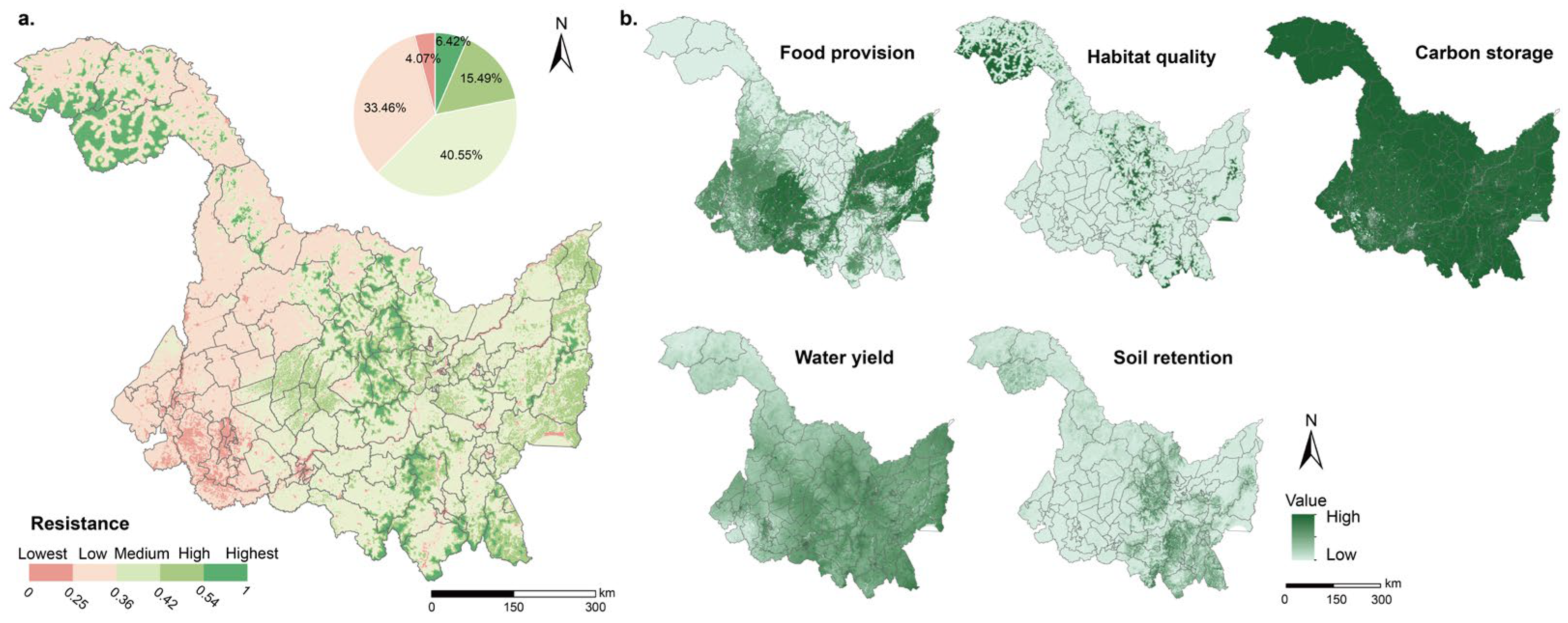
Resistance is mainly characterized by medium and low levels, which account for 40.55% and 33.46% of the total provincial administrative area, respectively, whereas high and highest levels together represent only 21.91% (Figure 3). Spatially, high resistance is primarily concentrated in the mountainous and forest-dominated areas of northern and eastern Heilongjiang, especially in the Greater and Lesser Khingan Mountains and other hilly areas with relatively intact ecological conditions. In contrast, low and lowest resistance is mainly distributed in the western and southwestern plains, as well as in agricultural and urbanized areas. These two categories together account for 37.53% of the provincial administrative area, including 33.46% for low resistance and 4.07% for lowest resistance. In these areas, ecosystem-service supply capacities, such as habitat quality, carbon storage, water yield, and soil conservation, are comparatively weak. This pattern indicates that the buffering capacity of ecological systems against external disturbances remains uneven across the province, with low-resistance areas largely corresponding to regions under stronger anthropogenic pressure and more intensive land development.

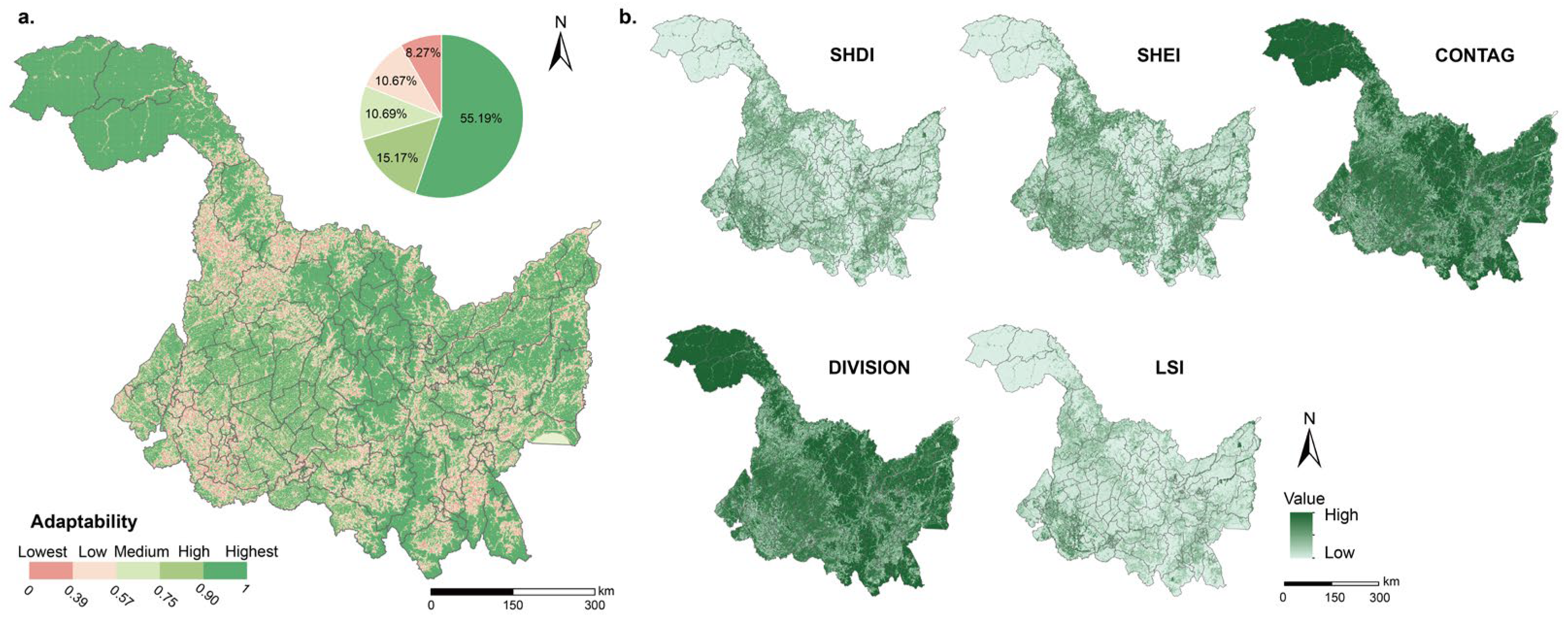
Adaptability shows a markedly stronger overall performance than resistance. The highest and high levels account for 55.19% and 15.17%, respectively, while the lowest and low levels represent only 8.27% and 10.67% (Figure 4). High adaptability areas are widely distributed across the province and are especially prominent in the northern forest regions, the eastern mountainous belt, and parts of the southern hilly areas. By contrast, relatively low adaptability is mainly found in the central-western agricultural plains and some urban-rural transition zones. These results suggest that, in most parts of Heilongjiang, landscape structure and spatial configuration provide relatively favorable conditions for ecological adjustment and reorganization. In particular, areas dominated by forest, grassland, and water patches tend to exhibit stronger adaptability, whereas highly cultivated and disturbed landscapes show comparatively lower adaptive capacity.

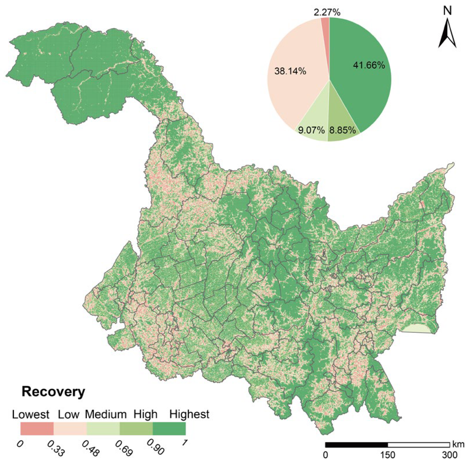
Recovery presents a more polarized spatial pattern than the other two dimensions (Figure 5). The highest level accounts for 41.66% of the province, while the low level also occupies a large proportion, reaching 38.14%; by comparison, the lowest, medium, and high levels account for only 2.27%, 9.07%, and 8.85%, respectively. High recovery areas are mainly concentrated in ecologically well-preserved mountainous and forested regions, especially in northern Heilongjiang and several eastern and southeastern counties. In contrast, low recovery areas are more common in the western and central plains and in intensively cultivated landscapes, where ecological systems are more vulnerable to long-term disturbance and show weaker post-disturbance restoration potential. This polarized pattern implies that the regenerative capacity of ecosystems in Heilongjiang is highly differentiated, with substantial contrasts between natural ecological strongholds and human-dominated production spaces.

4.1.2. Spatial Patterns of ER at the Grid and County Scales

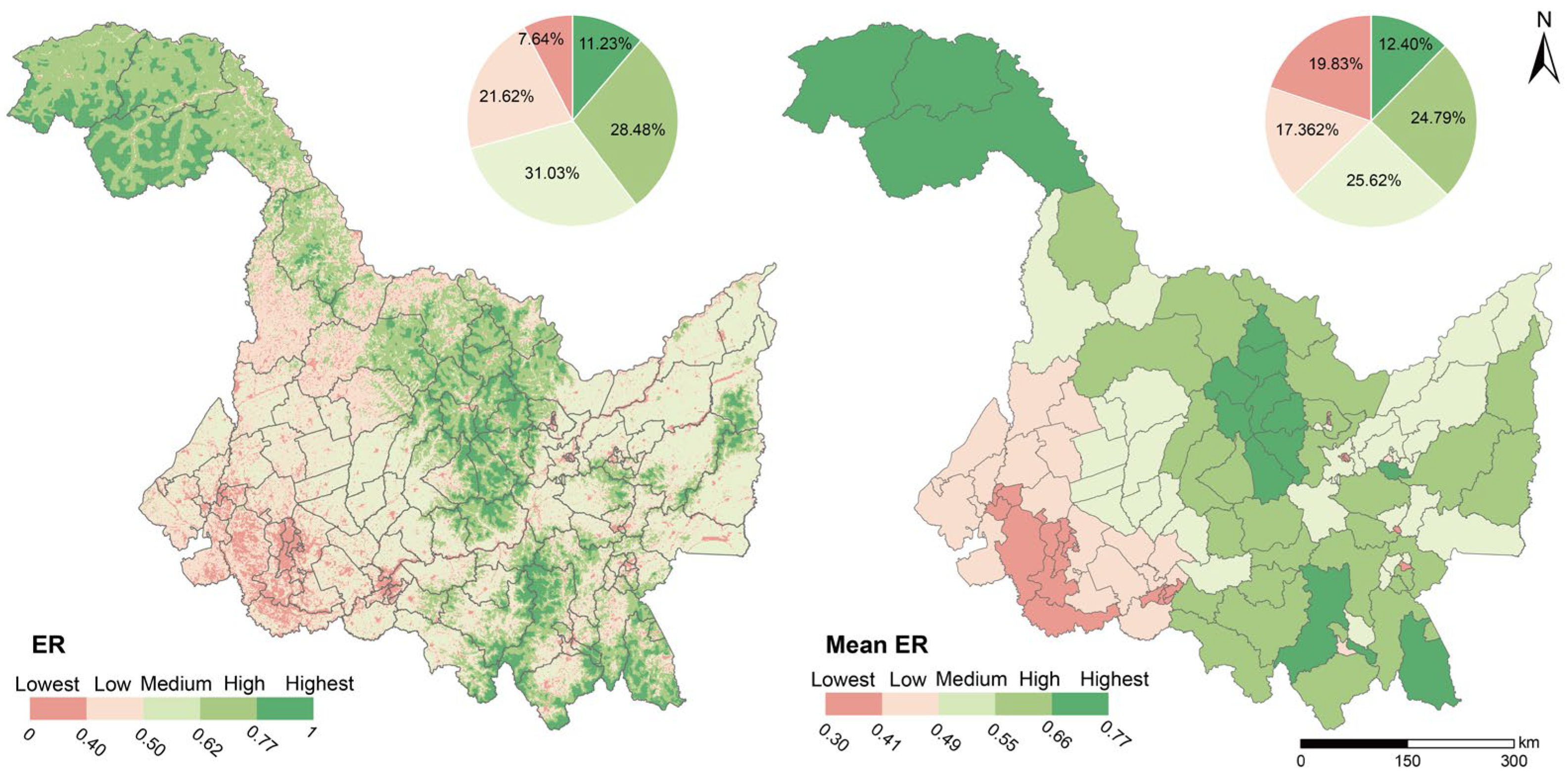
At both grid and county scales, ER exhibits a consistent northeast-to-southwest declining gradient across Heilongjiang Province, indicating scale-invariant spatial heterogeneity. At the 1 km grid scale, ER exhibits pronounced spatial heterogeneity across Heilongjiang Province (Figure 6). Medium and high levels dominate the overall pattern, accounting for 31.03% and 28.48% of the province, respectively, while the highest, low, and lowest levels account for 11.23%, 21.62%, and 7.64%. Spatially, high and highest ER values are mainly concentrated in mountainous and forest-dominated areas, particularly in the Greater and Lesser Khingan Mountains in northern Heilongjiang, as well as in several hilly and ecologically well-preserved areas in the central, eastern, and southeastern parts of the province. By contrast, low and lowest ER values are mainly distributed in the western and southwestern plains and in intensively cultivated and urbanized areas.

After aggregating the grid-level results to the county scale, ER continues to show clear spatial differentiation across the province. Medium and high levels account for 25.62% and 24.79% of counties, respectively, while the highest, low, and lowest levels account for 12.40%, 17.36%, and 19.83%. Counties with the highest ER are mainly distributed in the northern forest region and several eastern and southeastern counties, especially in the Daxing’anling and Yichun areas. By contrast, low-ER counties are mainly concentrated in the western and southwestern parts of the province, particularly in the prefecture-level areas of Daqing, Qiqihar, and Hegang, where plain landscapes, intensive agricultural production, urban concentration, and stronger human disturbance are more prominent.

4.2. Global Moran’s I and Hot Spot Analysis

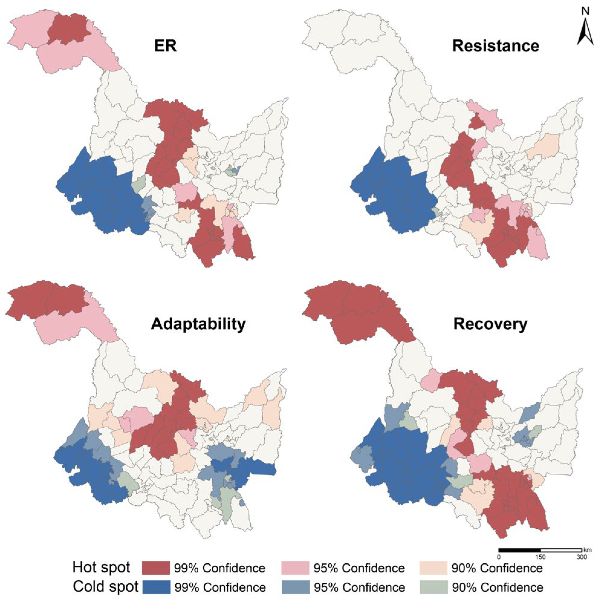
All four indicators exhibit significant positive spatial autocorrelation at the county scale (Global Moran’s I = 0.583 for resistance, 0.545 for ER, 0.526 for recovery, and 0.303 for adaptability; all p < 0.01). As shown in Figure 7, the cold spots are all concentrated in a contiguous belt in western and southwestern Heilongjiang, especially around the Qiqihar-Daqing region, indicating a pronounced low-value agglomeration in the western plain area. In contrast, hot spots are generally associated with the northern forest region, the central forest belt, and parts of southeastern Heilongjiang, reflecting the ecological advantages of mountainous and forest-dominated counties.

For ER, hot spots are mainly distributed in the northern forest region, the central forested belt, and several southeastern counties, whereas cold spots are concentrated in the western and southwestern counties. The spatial pattern of resistance is broadly similar to that of ER, although its hot spots are more concentrated in the central and southeastern forested areas, suggesting a stronger spatial concentration of buffering capacity in ecological strongholds. Compared with ER and resistance, adaptability shows a relatively more fragmented clustering pattern. Its hot spots are mainly located in the northern and central parts of the province, while some cold spots also appear in several eastern counties in addition to the western and southwestern cluster. By contrast, the spatial pattern of recovery is again closer to that of ER, with hot spots mainly concentrated in the northern forest region, the central forest belt, and the southeastern part of the province, and cold spots remaining strongly clustered in the west and southwest.

4.3. Spatial Patterns of Coupling Coordination Degree

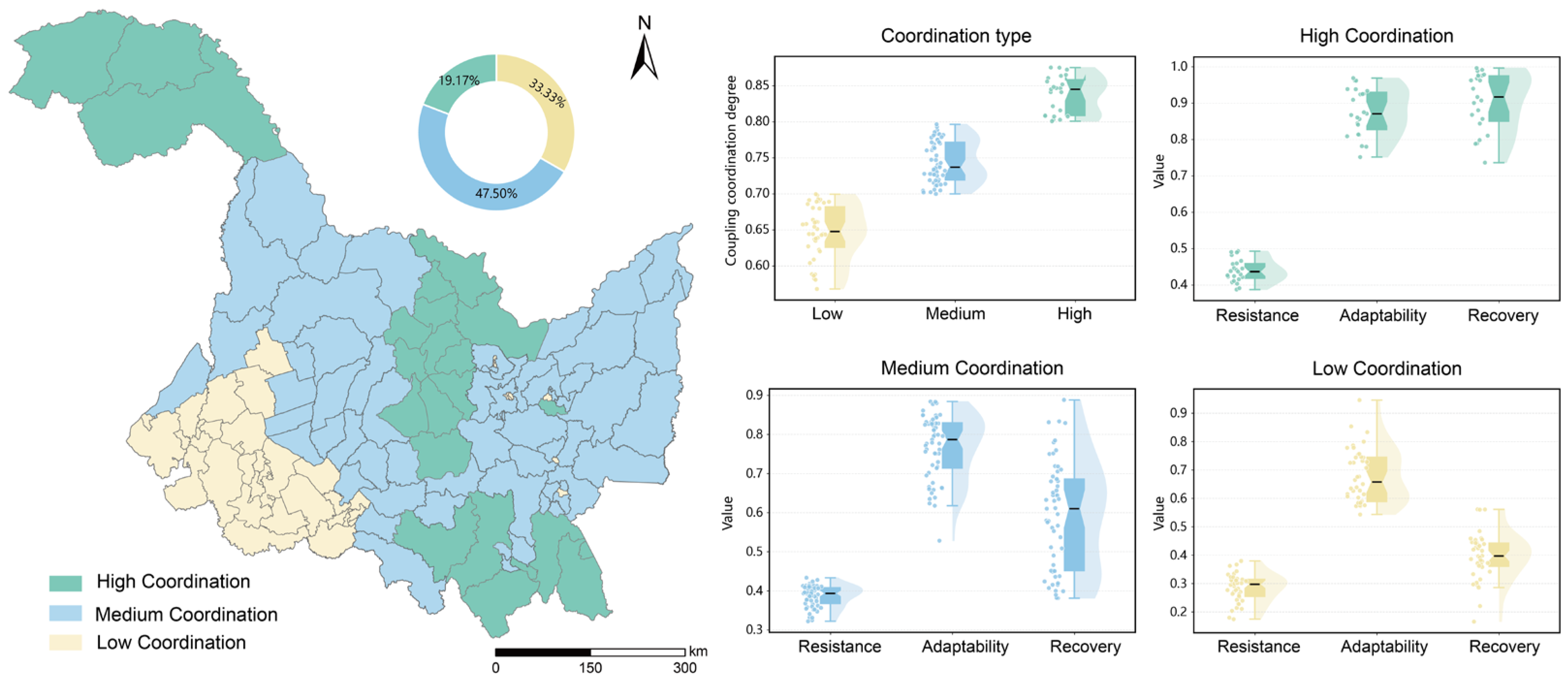
The coupling coordination among the three sub-dimensions of ecological resilience in Heilongjiang Province is dominated by medium coordination (47.50%), followed by low coordination (33.33%) and high coordination (19.17%), with coordination levels declining from the northeastern forested regions toward the western and southwestern plains (Figure 8). It indicates that 66.67% counties have entered a relatively coordinated state, although substantial spatial disparities remain. High-coordination counties are mainly distributed in the northern forest region and in several counties in central, eastern, and southeastern Heilongjiang. By contrast, low-coordination counties are concentrated in the western and southwestern parts of the province, forming a relatively contiguous low-value cluster. Medium-coordination counties occupy the largest proportion and are widely distributed across the central and eastern parts of Heilongjiang, constituting the transitional background of the provincial pattern.

The resistance, adaptability, and recovery also show distinct distributions across coordination types (Figure 8). In Figure 8, the dots represent individual county-level observations. The shaded violin plots depict the distribution and density of indicator values for each coordination category. In the high-coordination group, adaptability and recovery both maintain high levels, whereas resistance remains comparatively lower. In the medium-coordination group, adaptability is still relatively high, but recovery shows a much wider range and lower central tendency, suggesting that variation in recovery becomes an important source of differentiation within this type. In the low-coordination group, both resistance and recovery remain at relatively low levels, while adaptability is still moderate to relatively high. This pattern reveals that high coordination is not driven by synchronous strengthening of all three components, but by adaptability–recovery synergy, whereas low-coordination counties are constrained by persistently low resistance and recovery.

4.4. Obstacle Diagnosis of County-Level ER

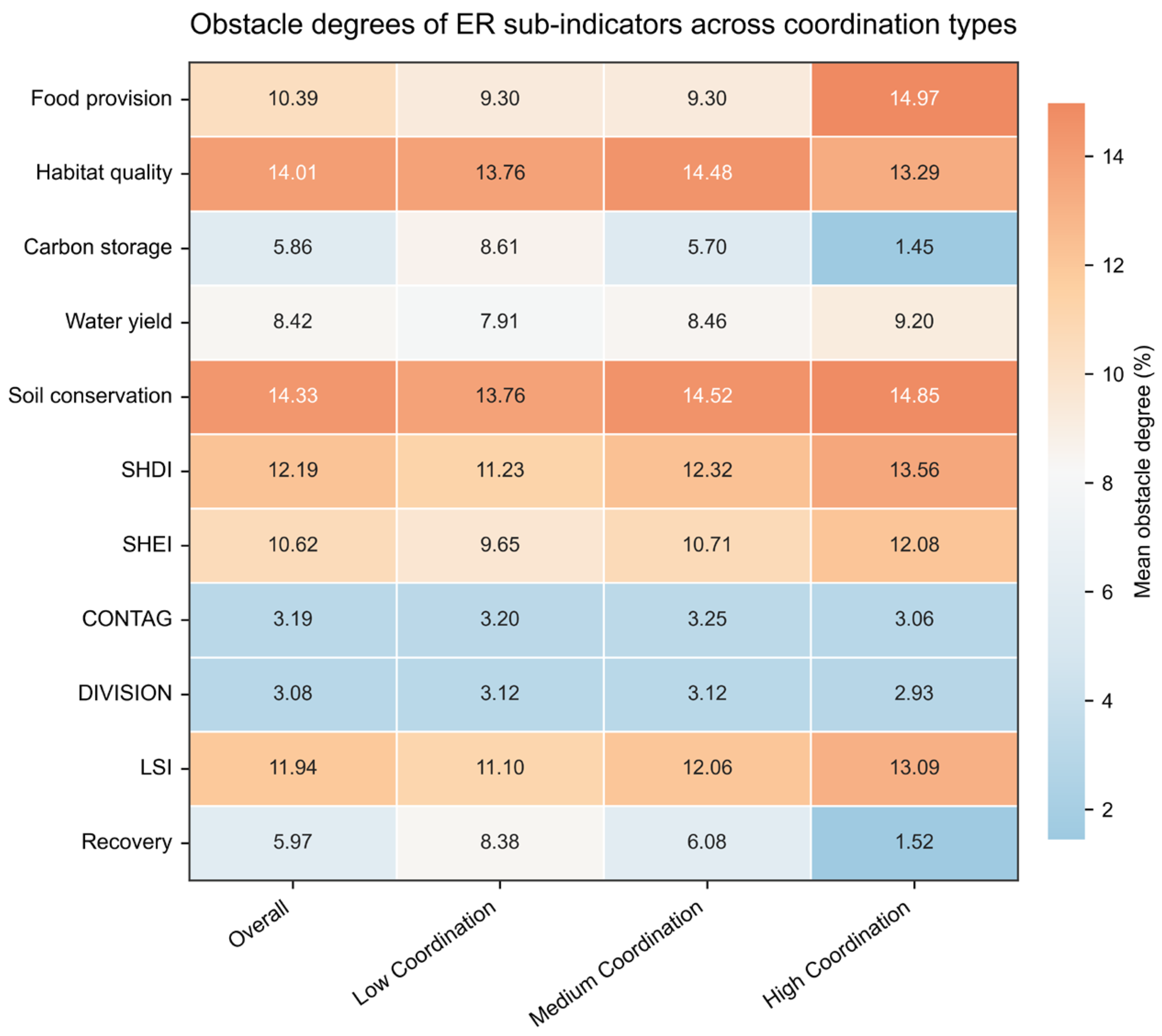
As shown in Figure 9, the obstacle structure of county-level ER in Heilongjiang Province is dominated by a limited number of sub-indicators. Overall, soil conservation and habitat quality are the two strongest obstacle factors, with mean obstacle degrees of 14.33% and 14.01%, respectively. They are followed by SHDI (12.19%), LSI (11.94%), SHEI (10.62%), and food provision (10.39%). By contrast, CONTAG (3.19%), DIVISION (3.08%), carbon storage (5.86%), and recovery (5.97%) show relatively lower obstacle degrees. This indicates that the main constraints on county-level ER mainly come from deficiencies in ecological service support and landscape structural characteristics, rather than from all sub-indicators simultaneously. The dominance of several key obstacle factors is evident across all 120 county-level units in Heilongjiang Province. Soil conservation is the primary obstacle in 69 counties (57.50%), habitat quality in 37 counties (30.83%), and grain production in 14 counties (11.67%). In other words, the obstacle pattern of county-level ER is highly concentrated, and most counties are primarily constrained by one of these three factors.

The obstacle composition further differs across coordination types. In the low-coordination group, habitat quality (13.76%) and soil conservation (13.76%) are the most important constraints. In the medium-coordination group, soil conservation (14.52%) and habitat quality (14.48%) remain the dominant obstacle factors, while SHDI (12.32%), LSI (12.06%), and SHEI (10.71%) also exert relatively strong constraints. In the high-coordination group, however, the obstacle structure shifts to some extent: grain production (14.97%) and soil conservation (14.85%) become the two leading constraints. At the same time, the obstacle degrees of carbon storage and recovery decline substantially in this group, at only 1.45% and 1.52%, respectively. This is because counties in the northeastern forested region maintain high carbon sequestration and ecological recovery capacity owing to their dense forest cover, and the remaining coordination gap in this group is therefore driven primarily by grain-production and soil-conservation deficits.

Overall, the obstacle diagnosis shows that county-level ER in Heilongjiang is mainly constrained by soil conservation, habitat quality, and several landscape-pattern indicators, whereas the roles of carbon storage, recovery, CONTAG, and DIVISION are comparatively weaker. As counties move toward higher coordination, the dominant constraints gradually shift from basic ecological support deficits toward a more composite obstacle structure involving both ecosystem services and landscape configuration.

5. Discussion

5.1. Spatial Differentiation and Coordinated Constraints of County-Level ER

The results reveal a highly differentiated spatial pattern of county-level ER in Heilongjiang, with consistently higher values in the northern and eastern forested and mountainous regions and lower values in the western and southwestern plains. Such a northeast-to-southwest declining ER gradient aligns with the ‘high-east, low-west’ pattern found in Jilin Province [49]. This pattern is already evident in the three components of resilience and is further reflected in the county-scale ER pattern, where high-ER counties are mainly distributed in the Daxing’anling and Yichun areas, while low-ER counties are concentrated in prefecture-level areas such as Daqing, Qiqihar, and Hegang. Taken together, these results suggest that the spatial differentiation of ER in Heilongjiang is associated with the joint effects of ecological background conditions, landscape structure, and the intensity of human disturbance. In the broader Northeast black soil region, land-use change, agricultural expansion, and the tension between food production and ecological integrity have already been shown to strongly reshape ecosystem-service patterns and ecological outcomes [50,51,52].

A first notable finding is that the three components of resilience do not perform synchronously. While the principle of asynchronous RAR development is consistent with findings in western strategic hinterlands of China [53], the specific dimensional bottlenecks differ across geographical contexts: adaptability lags in western inland provinces with stable resistance and rising recovery, whereas in Heilongjiang, resistance remains the relatively weaker dimension, with medium and low levels dominating the provincial pattern, whereas adaptability is generally high and recovery shows strong polarization. This indicates that counties in Heilongjiang are relatively better positioned in terms of ecological adjustment and landscape reorganization than in terms of disturbance buffering and post-disturbance regeneration. In ecological strongholds such as the northern forest regions, the combination of forest cover, relatively intact habitat conditions, and lower fragmentation likely provides a favorable basis for both adaptability and recovery, which is consistent with evidence from Heilongjiang and the Greater Khingan Mountains showing that natural forest protection and forest conservation have helped sustain forest ecosystems and reshape ecosystem-service trade-offs [51,54,55]. By contrast, in the western and southwestern plains, intensive cultivation, urban concentration, and stronger land-use disturbance appear to weaken both the buffering capacity of ecosystems and their long-term restorative potential. This interpretation is consistent with studies showing severe black-soil erosion in Northeast China [56], the growing need to reconcile agricultural modernization with black-soil protection in Heilongjiang [57], and the ecological vulnerability of cultivated-land systems in Qiqihar under intensive use [58]. This also helps explain why the spatial pattern of recovery is closer to that of ER than that of adaptability: in a province where ecological resilience is strongly conditioned by natural ecological endowments, regenerative capacity becomes a key factor differentiating relatively strong and weak counties.

Moreover, ER and its three components are not randomly distributed, but exhibit significant spatial clustering at the county scale, a pattern with implications for how ecological resilience should be governed across administrative boundaries. The Global Moran’s I values of ER, resistance, adaptability, and recovery are all positive and significant, and the hot spot analysis further shows that hot spots are generally associated with the northern forest region, the central forest belt, and parts of southeastern Heilongjiang, whereas cold spots are consistently concentrated in a contiguous belt across western and southwestern Heilongjiang, especially around the Qiqihar-Daqing region. This suggests that county-level ER in Heilongjiang is not only a function of local ecological conditions but also embedded in broader regional contexts. The spatial contiguity of cold spots is particularly consequential from a governance perspective: because low resilience is spatially cumulative rather than isolated, the ecological deficits of any single county are structurally entangled with those of its neighbors. This implies that county-level interventions are unlikely to be effective if implemented in isolation. Instead, the cold-spot belt calls for coordinated, multi-county governance mechanisms, including joint ecological compensation schemes, regionally harmonized land-use planning, and shared monitoring frameworks that transcend individual administrative units. Conversely, the spatial continuity of high-value clusters indicates that ecologically favorable counties benefit from mutually reinforcing regional conditions, including relatively intact forest ecosystems, better habitat continuity, and lower levels of anthropogenic fragmentation. Related studies in Northeast China similarly report pronounced regional ecological clustering and ecological security differentiation [58], while research in Harbin further shows that landscape-pattern change exerts strong spatially differentiated effects on ecosystem services and conservation priorities [59,60].

The coupling coordination results further deepen this understanding by showing that most counties have entered a medium-coordination state, while low-coordination counties remain concentrated in the west and southwest, and high-coordination counties are mainly distributed in the north and east. More importantly, the distributions of the three components across coordination groups indicate that counties with high coordination are supported by jointly high adaptability and recovery, whereas counties with low coordination are mainly constrained by low resistance and low recovery. This means that the improvement of county-level ER in Heilongjiang does not depend simply on raising all dimensions simultaneously. Instead, the main bottleneck lies in whether counties can strengthen the more deficient components—especially resistance and recovery—while maintaining the generally favorable performance of adaptability. In this sense, adaptability functions more as a broad provincial advantage, whereas resistance and recovery play a stronger role in determining whether counties can move to a higher coordination stage. This staged differentiation is also consistent with recent work in Heilongjiang and the broader black-soil region emphasizing coordinated development, black-soil protection, and the need to balance agricultural production with ecological integrity [57,61].

The obstacle diagnosis provides a more concrete explanation of these coordinated constraints. Overall, soil conservation and habitat quality are the strongest obstacle factors, followed by SHDI, LSI, SHEI, and grain production, while CONTAG, DIVISION, carbon storage, and recovery show relatively weaker average obstacle degrees. Unlike findings from the Yellow River Basin of China that identified hypervariation density, population density and GDP as the dominant drivers of ecological resilience, soil conservation and habitat quality emerged as the binding constraints in Heilongjiang that reflect the distinctive role of black-soil degradation and forest-edge habitat fragmentation in cold-region ecosystems [62,63]. The co-occurrence of these two deficits is not coincidental: both are downstream consequences of the same land-use trajectory; agricultural intensification has simultaneously eroded soil integrity and compressed habitat space. Moreover, the dominant constraints vary across coordination groups: low- and medium-coordination counties are mainly constrained by habitat quality, soil conservation, and several landscape-pattern indicators, whereas in high-coordination counties, grain production becomes more prominent together with soil conservation and landscape structure. The prominence of grain production as a constraint in this group is not a sign of agricultural underperformance, but rather a structural tension between the region’s ecological endowment and the food-provision demands placed on it. This pattern suggests that the key constraint on ER in Heilongjiang is not merely the absolute scarcity of ecological resources, but the mismatch between ecological support capacity and landscape organization. In relatively weak counties, deficits in core ecological support functions still dominate. In relatively strong counties, however, the limiting factors shift toward a more composite set of trade-offs involving ecological services, productive land use, and spatial configuration. Therefore, the transition from low to high ER coordination is not a linear process of universal improvement, but rather a staged shift in the nature of dominant constraints. This interpretation is well aligned with evidence from Harbin showing that landscape metrics such as diversity and configuration are closely linked to ecosystem-service responses [61], with scenario studies from the Northeast black soil region showing that land-management decisions reshape ecosystem sustainability and service provision [64], and with regional conservation assessments indicating that soil conservation remains a priority ecological function in Northeastern China [51].

5.2. Policy Implications for Improving County-Level ER

This study established a differentiated governance framework based on coordination types and dominant barrier structures, enabling strategies for improving county-level ER in Heilongjiang Province to go beyond mere ecological restoration, shifting from descriptive assessment to actionable diagnosis, distinguishing it from previous studies that only reported overall resilience scores. Since low-value clusters and low-coordination counties are spatially concentrated in the western and southwestern plains, while high-value clusters are concentrated in northern and eastern ecological strongholds, county-level policy should prioritize region-specific interventions rather than province-wide homogeneous targets [59,60,62].

For low-coordination counties, especially those located in the western and southwestern plains, the policy priority should be to address the basic ecological deficits that most directly constrain ER. Given that habitat quality and soil conservation are the dominant obstacle factors in this group, the first task is to strengthen ecological infrastructure in agricultural and urbanizing landscapes. Soil erosion in the black soil region of Northeast China shows a clear west–east differentiation, and Heilongjiang also faces the challenge of coordinating agricultural modernization with black-soil protection, which means that controlling soil erosion and reducing land-use pressure should be treated as priority tasks in these counties [56,57]. Improving cultivated-land ecological resilience in areas such as Qiqihar also requires reducing the ecological vulnerability of production spaces rather than simply expanding ecological land [58]. Future management should incorporate soil conservation measures, such as conservation tillage, vegetation buffer strips, and dynamic erosion-monitoring networks, to build long-term resilience against climatic and anthropogenic pressures.

For medium-coordination counties, which constitute the largest share of Heilongjiang, the policy focus should shift from basic remediation toward structural optimization. These counties already possess a relatively favorable adaptive basis but remain constrained by soil conservation, habitat quality, and landscape-pattern indicators such as SHDI and LSI. This means that the key task is to improve the spatial organization of ecological and production land, including optimizing the layout of woodland, farmland, wetlands, and built-up land, reducing excessive landscape fragmentation, and improving the connectivity and heterogeneity of ecological patches [61,62]. In agricultural counties, this may require integrating high-standard farmland construction with ecological buffer design, while in resource-based or transition counties it may involve ecological restoration of abandoned industrial land and more efficient reuse of underutilized spaces [52]. Future spatial planning should adopt a multi-functional landscape design paradigm, integrating ecological corridors and agro-ecological zoning and enhancing connectivity so that landscape configuration evolves proactively from passive remediation toward strategically engineered adaptability.

For high-coordination counties, many of which are located in the northern forest region and ecologically favorable eastern areas, the main task is to consolidate existing advantages while preventing new constraints from emerging. In this group, grain production becomes a more important obstacle factor, while landscape structure and soil conservation remain key concerns. This suggests that even ecologically strong counties face the challenge of balancing ecological protection with production demands. Policy in these counties should therefore emphasize maintaining forest integrity, protecting key ecosystem-service areas, and preventing new fragmentation caused by expansion-oriented development [54,55]. Given that soil conservation is identified as a future conservation priority in Northeastern China, these counties should also strengthen the coordinated management of ecological conservation and agricultural or forestry production rather than pursuing further land expansion [51].

At the provincial scale, the pronounced cold-spot concentration in western and southwestern Heilongjiang also suggests the need for a regional coordination mechanism. Since low-ER counties form a contiguous belt rather than isolated cases, ecological governance should be organized not only at the county level but also across county boundaries. A cross-county governance framework around western plain ecological restoration, water-soil conservation, and agricultural landscape optimization would help neighboring counties facing similar constraints coordinate restoration targets and monitoring systems [59]. At the same time, ecological management zoning and conservation prioritization should be strengthened so that northern and eastern ecological strongholds can be treated as key ecological sources whose benefits extend beyond individual administrative units [60,62,65]. Crucially, future provincial governance should establish a province-wide adaptive monitoring system that integrates remote-sensing surveillance, ground-based ecological indicators, and periodic county-level resilience reassessment to adjust relative policies.

5.3. Limitations and Prospects

This study has several limitations. First, aggregating grid-scale indicators to administrative units introduces the Modifiable Areal Unit Problem (MAUP), which may attenuate within-county heterogeneity and produce scale-dependent statistical relationships. Although the county scale is appropriate for identifying broad regional patterns and supporting county-level governance, administrative boundaries do not exactly match the ecological boundaries. Additionally, the aggregation of 1 km grid results may mask important within-county heterogeneity, especially in counties that contain both ecological core areas and highly disturbed production spaces. Future research could analyze watershed or eco-functional zonation boundaries, combined with finer-scale hotspot identification, to improve both the spatial precision of governance [54]. Second, uncertainties remain in the ecosystem-service assessment. The InVEST-based estimates may be overestimated or underestimated because the model simplifies ecological and hydrological processes and partly relies on literature-based or regional-average parameters. Future studies should incorporate locally calibrated parameters, field observations, and process-based model comparisons to improve estimation accuracy. Third, the present analysis mainly reveals spatial patterns, coordination states, and dominant obstacle factors but does not fully identify the causal mechanisms through which natural conditions, landscape structure, and human disturbance jointly shape ER. Future studies could introduce explanatory models to further test the relative contributions and interactions of these drivers [66]. Finally, this study is based on a cross-sectional assessment for 2024 and therefore focuses more on spatial differentiation than on temporal evolution. Since county-level ER is inherently dynamic, future research should extend the framework to a multi-period perspective in order to examine how ER, coordination types, and dominant obstacle factors change over time.

6. Conclusions

The results of this study indicate that the three dimensions of ecological resilience (resistance, adaptability, and recovery) in Heilongjiang Province exhibit distinct spatial patterns: resistance is relatively weak overall, adaptability performs comparatively well, and recovery shows a strongly polarized distribution. The results show that the three components exhibit distinct spatial patterns: resistance is relatively weak overall, adaptability performs comparatively well, and recovery shows a strongly polarized distribution. At the county scale, ER displays a clear spatial gradient, with relatively high values concentrated in the northern and eastern forested and mountainous areas, especially the Daxing’anling and Yichun regions, while low-value counties are mainly distributed in the western and southwestern plains, particularly around Daqing, Qiqihar, and Hegang.

County-level ER and its three components all exhibit significant positive spatial autocorrelation, and their hot spots and cold spots form clear regional clusters. Cold spots form a contiguous belt across western and southwestern Heilongjiang, while hot spots cluster in the northern, central, and southeastern forested regions. Of all counties, 47.50% are in medium coordination; high-coordination counties depend on the joint support of adaptability and recovery, whereas low-coordination counties are primarily constrained by deficits in resistance and recovery.

County-level ER in Heilongjiang is mainly constrained by soil conservation, habitat quality, and several landscape-pattern indicators, especially SHDI, LSI, and SHEI, while the roles of CONTAG, DIVISION, carbon storage, and recovery are comparatively weaker. Dominant obstacles vary across coordination types: low- and medium-coordination counties are primarily limited by habitat quality, soil conservation, and landscape configuration, whereas in high-coordination counties, grain production becomes more prominent together with soil conservation and landscape structure. These results suggest that the improvement of county-level ER in Heilongjiang should move beyond uniform ecological restoration and instead adopt differentiated governance strategies targeting the dominant constraints of different county groups. Improving county-level ER in Heilongjiang, therefore, requires differentiated governance targeting each county group’s dominant constraints rather than uniform ecological restoration.