Localisation of Sustainable Development Goals in the Regions of Russia and Kazakhstan: Comparative Analysis and Factors of Spatial Differentiation

Abstract

The article presents the results of an empirical study of the localisation processes of the Sustainable Development Goals (SDGs) in 102 regions of Russia and Kazakhstan for the period 2015–2024. Based on the author’s methodology for constructing the SDG Localisation Index (SDGLI) using the method of the main components, a quantitative assessment of regional progress was carried out according to 14 SDGs. Cluster analysis has identified four sustainable types of regions that differ in the structure and dynamics of sustainable development. Using eco-metric tools (panel regressions with fixed effects, spatial models, difference-in-differences method), key factors of interregional differentiation were identified, including economic, social, institutional and spatial determinants. Particular attention is paid to assessing the effect of adopting regional sustainable development strategies. A decomposition of interregional inequality was carried out, which made it possible to quantify the contribution of various groups of factors. The results of the study contribute to the theory of regional economics and can be used to improve regional policies in the field of sustainable development.

1. Introduction

The relevance of the research on the processes of localisation of the Sustainable Development Goals (SDGs) at the subnational level is due to the approaching deadline for the implementation of Agenda 2030 and the need to comprehend the interim results of the implementation of global goals in countries with different government structures.

Following the definition by UN-Habitat and the Sustainable Development Solutions Network (SDSN), “SDG localisation” is understood as a multi-level process that involves adapting global SDG targets and indicators to subnational contexts, taking into account regional priorities, institutional capacities, and stakeholder participation [1]. This concept implies the translation of global goals into regional strategies, the selection of locally relevant indicators, and the alignment of regional policies with the SDG framework.

In modern international discourse, localisation of the SDGs is considered a multi-level process that requires coordination of global indicators with national priorities and local conditions, taking into account regional specifics and involving a wide range of stakeholders [2,3]. A key localisation tool is Voluntary Local Reviews (VLRs), which allow subnational authorities to assess progress towards the SDGs and present results at the international level [4]. The effectiveness of the implementation of the SDGs largely depends on the consistency of policies at different levels of government, which is confirmed by studies of political coherence [5]. Global action to achieve the SDGs in the post-pandemic period also requires a review of monitoring and evaluation approaches [6].

Comparative analysis of Russia and Kazakhstan in the context of SDG localisation is of special scientific and practical interest. Both countries, being members of the Eurasian Economic Union and preserving a common historical heritage, demonstrate different models of state structure and regional policy. Russia is a federation with constitutionally enshrined budgetary powers of the regions, while Kazakhstan is a unitary state with a high degree of centralisation of government. The researchers note that the post-Soviet states are characterised by a vertical model of the implementation of the SDGs, where the regions act mainly as executors of federal decisions, and not as independent subjects of goal-setting [7]. A comparative analysis of approaches to the institutionalisation of the SDGs at the regional level in the two countries reveals differences in formal institutional practices, the choice of priority goals and the resourcing of management decisions [8].

Issues of legal regulation and public policy in the field of environmental management in the context of achieving the SDGs also reveal country specifics. Studies show that there are many contradictory acts in Russian legislation, while Kazakhstan’s strategic documents are more coordinated. At the same time, in both countries there is no normative consolidation of instruments for achieving the SDGs at the regional level, and fragmented and inconsistent approaches enshrined in policy documents cause duplication of individual provisions [9]. According to policy documents and analytical reviews, limited localisation of the SDGs, especially at the regional and municipal levels, remains one of the key structural problems in Kazakhstan [10]. An important role in promoting SDG localisation is played by research centres and civil society organisations that develop a public monitoring methodology that allows assessing progress on the SDGs in terms of service accessibility, barriers and perceptions of equity [11]. The Voluntary National Review of Kazakhstan records continuing structural challenges: limited SDG localisation, insufficient policy coherence between sectors, and weak monitoring and accountability mechanisms.

Experts also point to problems associated with inadequate logistics infrastructure and a high concentration of trade in the commodity sector, which limits economic diversification and the achievement of Sustainable Development Goal 9 (SDG 9) in the North and Central Asia region [12]. The theoretical and methodological basis of the study is work in the field of regional economics and spatial analysis.

In the international literature, considerable attention is paid to the application of spatial econometric methods [13], the methodology for evaluating panel data with bilateral effects [14], as well as the analysis of economic convergence [15], which offers approaches applicable to the study of regional differentiation. In the Russian scientific tradition, the problems of sustainable development of regions are being developed in line with studies of regional differentiation and spatial inequality. A significant contribution was made by works devoted to the construction of integral indices of socio-economic development [16], an integral assessment of the economic development of the regions of the Russian Federation [17], an analysis of interregional convergence [18], and employment modelling using spatial-econometric methods [19]. The researchers also made a significant contribution to the study of agglomeration effects in the regional economy [20,21], the analysis of agglomeration effects as a tool for regional development [22], and the development of a methodology for assessing spatial interactions based on global and local Moran’s I statistics (measures of spatial autocorrelation) [23]. A comprehensive analysis of the innovative development of Russian regions in the context of sustainable development [24], a study of theoretical and methodological approaches to the study of depressed regions [25,26], the development of a methodological approach to assessing the effectiveness of public administration in the regions [27], as well as theoretical and methodological foundations for studying the sustainable development of regions [28] create the necessary basis for conducting this research.

The practice of preparing voluntary local reviews in Russia and Kazakhstan is only being formed. According to analytical materials, Russian VLRs demonstrate a high level of data elaboration, but they face the problem of comparability with international indicators and limited impact on budget planning [29]. According to international data, to date, more than 250 cities and regions of the world have submitted VLR, but in the Commonwealth of Independent States (CIS) this practice is in its infancy [30]. The CIS Interstate Statistical Committee monitors SDG indicators in the region, providing methodological and statistical support to the participating countries [31].

The fundamental foundations of the study of inequality and institutional development are laid in works analysing the interaction of the state and society in the context of freedom and development [32], as well as in works proposing practical measures to reduce inequality [33]. Despite the presence of a significant number of studies on certain aspects of sustainable regional development, comprehensive comparative studies of SDG localisation processes in Russia and Kazakhstan using modern econometric tools, including spatial models and methods for assessing causal effects, have not yet been available. This determines the need for this research.

The purpose of this article is to compare the processes of localisation of the Sustainable Development Goals in the regions of Russia and Kazakhstan, to identify key factors determining interregional differences, and to assess the effectiveness of regional sustainable development strategies.

To achieve this goal, the following tasks are being solved, each linked to the corresponding research hypotheses (H1–H6):

(1)

The development of an integral index of SDGs localisation based on a two-level PCA (supports H1, H2);

(2)

Cluster analysis of regions according to the structure of progress in achieving the SDGs (provides empirical basis for H4, H5);

(3)

Econometric modelling of interregional differentiation factors using panel data and spatial specifications (tests H1, H2, H4);

(4)

Assessment of the causal effect of adopting regional sustainable development strategies using the difference-in-differences method (tests H3);

(5)

Decomposition of interregional inequalities, highlighting the contribution of economic, social, institutional and spatial factors (tests H6);

(6)

Comparative analysis of two models of SDGs localisation in Russia and Kazakhstan (tests H5).

The scientific novelty of the study lies in the development of a comprehensive methodology for assessing the localisation of the SDGs at the regional level, first used for a comparative analysis of the regions of Russia and Kazakhstan; in the identification of stable types of regions by the structure of progress with the identification of the phenomenon of the “paradox of poor inequality” (i.e., the poorest regions exhibit unexpectedly low within-region inequality, often due to homogeneous low incomes); in quantifying interregional differentiation factors using modern econometric instrumentation, including spatial models and methods for estimating causal effects; in the decomposition of interregional inequality, highlighting the contribution of various groups of factors; in identifying and meaningfully interpreting differences in SDGs localisation models in the two countries.

Research Hypotheses

Based on the theoretical framework and the aims of the study, the following hypotheses are formulated:

H1. 

Economic factors, particularly Gross Regional Product (GRP) and investment in fixed assets, have a positive and dominant effect on the SDG localisation index (SDGLI), outweighing the contribution of social and institutional factors.

H2. 

Institutional quality (IQI), measured through fiscal autonomy, budget discipline, corruption prevalence, digitalisation of public services, SME density, and public administration employment, positively influences SDGLI, and this effect remains significant after controlling for economic development.

H3. 

The adoption of a regional sustainable development strategy (Policy) exerts a positive causal effect on SDGLI, but this effect is not immediate: it manifests with a time lag of one to two years and strengthens over subsequent periods.

H4. 

There exist positive spatial spillovers in SDG localisation: improvements in neighboring regions’ SDGLI lead to an increase in the index in a given region, indicating diffusion of successful practices and policies.

H5. 

The models of SDG localisation differ between Russia and Kazakhstan: Kazakhstan demonstrates higher growth rates of SDGLI but stronger interregional inequality (higher coefficient of variation), while Russia exhibits more spatially even development and greater reliance on accumulated human capital.

H6. 

The contribution of economic factors to interregional inequality in SDGLI is larger than that of social, institutional, or spatial factors, with Gross Regional Product (GRP) per capita being the single most important contributor.

2. Materials and Methods

2.1. Research Design and Data

The study employs quantitative methods of multidimensional statistics, econometric modelling, and spatial analysis. The observation period covers 2015–2024. The spatial sample includes 89 regions of the Russian Federation (as of 2024) and 17 regions of the Republic of Kazakhstan (14 oblasts and three cities of republican significance—Astana, Almaty, Shymkent). After harmonising statistical indicators (see Section 2.2.2), a balanced panel of 102 spatial units over 10 time periods was obtained, giving 1020 observations.

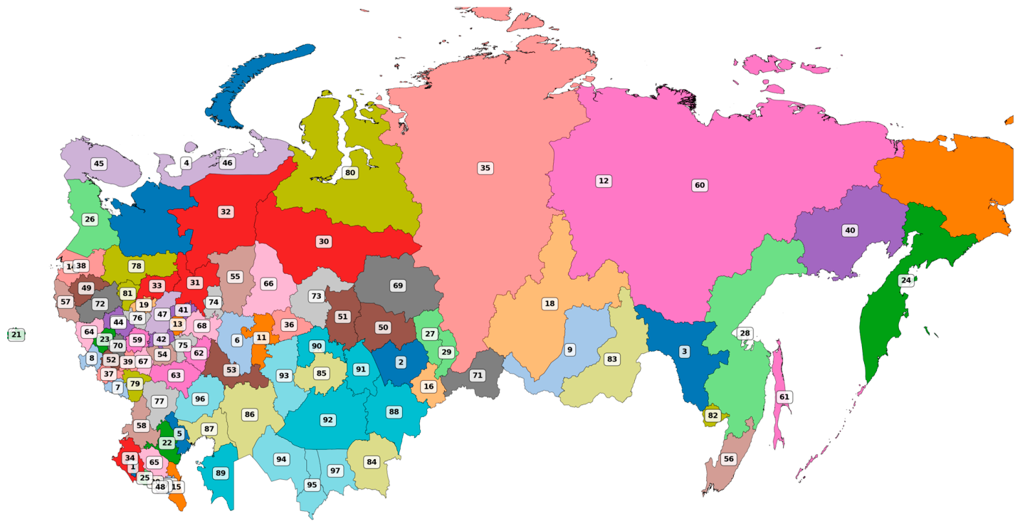
The spatial distribution of the analysed regions is shown in Figure 1.

The information base consists of three groups of sources.

(i)

National official statistics: Rosstat data, including the Unified Interdepartmental Information and Statistical System and specialised SDG regional compendia [34]; data from the Bureau of National Statistics of Kazakhstan, including the “Regions of Kazakhstan” compendium and departmental reports [35].

(ii)

Financial and administrative data: Federal Treasury of Russia on consolidated regional budget execution [36]; Ministry of Finance of Kazakhstan on local budgets [37]; Committee on Legal Statistics of Kazakhstan on corruption offences [38].

(iii)

International databases: UN SDG Database [39], World Development Indicators [40], and OECD Regional Database [41], used for cross-validation.

2.2. Construction of the Subnational SDG Localisation Index (SDGLI)

The SDGLI is a composite index constructed using a two-level principal component analysis (PCA) approach, adapted from the Sustainable Development Solutions Network (SDSN) global ranking methodology [42,43].

2.2.1. Indicator Selection

Forty-seven indicators were selected across 14 SDGs based on relevance, data availability, cross-country comparability, discriminatory power, and balance among economic, social and environmental dimensions. Excluded goals were SDG 14 (marine ecosystems, lacking regional dimension) and several targets that have no regional disaggregation (e.g., some targets under SDG 2 and SDG 6, as well as SDG 17, which is national by nature). The full indicator list is given in

Table A1. System of indicators for calculating the subnational SDG Localisation Index (SDGLI).

SDG	Goal Name	Number of Indicators	Examples of Indicators
SDG 1	No Poverty	4	Share of population with income below the subsistence minimum, %; share of population receiving social support measures, %; unemployment rate, %; coverage of population with targeted social assistance, %
SDG 3	Good Health and Well-being	5	Life expectancy at birth, years; infant mortality rate, per 1000 live births; mortality from circulatory system diseases, per 100,000 population; number of physicians per 10,000 population; tuberculosis incidence, per 100,000 population
SDG 4	Quality Education	4	Coverage of children with preschool education, %; share of 9th-grade graduates receiving a certificate, %; share of employed persons with higher education, %; number of university students per 10,000 population
SDG 5	Gender Equality	3	Share of women in regional legislative bodies, %; ratio of women’s to men’s wages; share of women in managerial positions, %
SDG 6	Clean Water and Sanitation	3	Share of population supplied with quality drinking water, %; share of population served by centralised sewerage, %; share of wastewater treated to regulatory standards, %
SDG 7	Affordable and Clean Energy	3	Share of population supplied with natural gas, %; electricity consumption per capita, kWh; share of households using electricity for heating, %
SDG 8	Decent Work and Economic Growth	5	Gross Regional Product (GRP) per capita (PPP), USD; labour productivity, thousand RUB/person; employment rate, %; share of fixed capital investment in GRP, %; share of small and medium-sized enterprises in employment, %
SDG 9	Industry, Innovation and Infrastructure	4	Share of paved roads, %; number of broadband internet subscribers per 100 people; share of manufacturing in GRP, %; freight turnover of road transport, million t·km
SDG 10	Reduced Inequalities	3	Gini coefficient; income ratio of the top 10% to the bottom 10% of the population, times; income concentration index
SDG 11	Sustainable Cities and Communities	4	Share of population living in dilapidated housing, %; share of urban population with access to public transport, %; level of housing amenities, %; air pollutant emissions from motor vehicles per capita, kg
SDG 12	Responsible Consumption and Production	2	Generation of production and consumption waste per capita, tonnes; share of waste that is recycled, %
SDG 13	Climate Action	2	Air pollutant emissions per unit of GRP, tonnes/million RUB; Energy intensity of GRP, tce/million RUB
SDG 15	Life on Land	3	Share of specially protected natural areas in the region’s area, %; forest cover of the territory, %; reforestation, ha per 1000 ha of forest land
SDG 16	Peace, Justice and Strong Institutions	2	Number of recorded crimes per 1000 people; share of population satisfied with the work of local authorities, %

(Appendix A).

2.2.2. Data Harmonisation and Preprocessing

To ensure comparability between Russian and Kazakhstani data, the following procedures were applied. All monetary values were converted to constant 2015 US dollars at purchasing power parity using World Bank conversion factors and regional GRP deflators. Methodological harmonisation of poverty, unemployment and education indicators followed the recommendations of the CIS Interstate Statistical Committee. Missing values were imputed by linear interpolation for gaps ≤ 2 consecutive years, and by k-nearest neighbours (k = 5, Euclidean distance on structural characteristics) for isolated spatial gaps. Regions with >15% missing data were excluded. Outliers, identified using the interquartile range method (Tukey’s fences) with a coefficient of 3, were winsorised to the 1st and 99th percentiles.

2.2.3. Normalisation

All indicators were normalised to a [0,100] scale using min-max transformation with global fixed boundaries determined from the entire panel.

For stimulants (higher original value indicates better performance):

$$x_{ijt}^{\mathrm{norm}}={\displaystyle \frac{x_{ijt}-\underset{j}{\mathrm{m}\mathrm{i}\mathrm{n}}\left(x\right)}{\underset{j}{\mathrm{m}\mathrm{a}\mathrm{x}}\left(x\right)-\underset{j}{\mathrm{m}\mathrm{i}\mathrm{n}}\left(x\right)}}\times 100,$$

(1)

where $x_{ijt}$ is the original value of indicator $j$ for region $i$ in year $t$; ${\mathrm{m}\mathrm{i}\mathrm{n}}_j\left(x\right)$ and $\underset{j}{\mathrm{m}\mathrm{a}\mathrm{x}}\left(x\right)$ are the global minimum and maximum of indicator $j$ over all observations (all regions, all years); $x_{ijt}^{\mathrm{norm}}$ is the normalised value.

For destimulants (lower original value indicates better performance):

$$x_{ijt}^{\mathrm{norm}}={\displaystyle \frac{\underset{j}{\mathrm{m}\mathrm{a}\mathrm{x}}\left(x\right)-x_{ijt}}{\underset{j}{\mathrm{m}\mathrm{a}\mathrm{x}}\left(x\right)-\underset{j}{\mathrm{m}\mathrm{i}\mathrm{n}}\left(x\right)}}\times 100,$$

(2)

where the notation is the same as in Equation (1).

2.2.4. Weighting and Aggregation

A two-level PCA is employed: first, to derive weights of indicators within each SDG; second, to derive weights of the SDGs in the final index.

Standardisation prior to PCA. Before each PCA, variables are standardised to zero mean and unit variance:

$$z_{ijt}={\displaystyle \frac{x_{ijt}^{\mathrm{norm}}-{\stackrel{\text{-}}{x}}_j}{{\sigma }_j}},$$

(3)

where ${\stackrel{\text{-}}{x}}_j={\displaystyle \frac{1}{N}}{\sum }_{i,t}{x}_{ijt}^{\mathrm{norm}}$ is the mean of indicator $j$ over the entire panel ($N=1020$, i.e., 102 regions × 10 years), ${\sigma }_{j }$ is its standard deviation, and $z_{ijt}$ is the standardised value. Standardisation to zero mean and unit variance is a standard preprocessing step for PCA and does not require the data to be normally distributed; it ensures that all indicators contribute equally regardless of their original scales. The standardised values $z_{ijt}$ are then used to construct the correlation matrix $R_k$ for the first-level PCA (see Equations (4) and (5)).

First-level PCA (within each SDG): For each SDG $k$ with $p_k$ indicators, let $Z_k$ be the $n\times p_k$ matrix of standardised values. Here $n=1020$ (102 regions × 10 years). The correlation matrix is $R_k={\displaystyle \frac{1}{n-1}}{Z}_k^T{Z}_k$. Solve the eigenvalue problem:

$$R_k{v}_{km}={\lambda }_{km}{v}_{km},$$

(4)

where ${\lambda }_{k1}\ge {\lambda }_{k2}\ge \cdots \ge {\lambda }_{k{p}_k}$ are the eigenvalues (variances of the principal components), and $v_{km}$ are the corresponding eigenvectors (loadings). Here $v_{km}=(v_{km1},v_{km2},\dots ,v_{km{p}_k}{)}^T$ is the eigenvector for the eigenvalue ${\lambda }_{km}$, with $m\in \{\mathrm{1,2},\dots ,p_k\}$. The first principal component (PC1) loadings are used, i.e., $v_{k1}$. Denote by $v_{k1j}$ the $j$-th component of this eigenvector.

The weight of indicator $j$ within SDG $k$ is as follows:

$$w_{jk}={\displaystyle \frac{{\left(v_{k1j}\right)}^2}{{\displaystyle {\sum }_{l=1}^{p_k}}{\left(v_{k1l}\right)}^2}},$$

(5)

where $v_{k1j}$ is the loading of indicator $j$ on PC1 for SDG $k$; $p_k$ is the number of indicators in SDG $k$; $w_{jk}$ is the normalised weight (${\sum }_{j=1}^{p_k}{w}_{jk}=1$).

The subindex for SDG $k$ in region $i$ and year $t$ is as follows:

$$SD{G}_{kit}={\displaystyle \sum _{j=1}^{p_k}}{w}_{jk} x_{ijt}^{\mathrm{norm}},$$

(6)

where $x_{ijt}^{\mathrm{norm}}$ is the normalised value from Equation (1) or Equation (2).

Second-level PCA (across SDGs): Apply PCA to the $n\times 14$ matrix of subindices $SD{G}_{kit}$ (with $n=1020$). Let $v_{1k}^{\left(2\right)}$ be the loading of SDG $k$ on the first principal component of this second-level PCA. Note that $v_{1k}^{\left(2\right)}$ is a scalar (the $k$-th component of the first eigenvector), not a vector; therefore $\left(v_{1k}^{\left(2\right)}{)}^2\right.$ is well-defined.

The weight of SDG $k$ in the integral index is as follows:

$$w_k={\displaystyle \frac{\left(v_{1k}^{\left(2\right)}{)}^2\right.}{{\displaystyle {\sum }_{k=1}^{14}}({v_{1k}^{\left(2\right)})}^2}},$$

(7)

where $w_k$ satisfies ${\sum }_{k=1}^{14}{w}_k=1$.

The final SDGLI for region $i$ in year $t$ is as follows:

$$SDGL{I}_{it}={\displaystyle \sum _{k=1}^{14}}{w}_k SD{G}_{kit}.$$

(8)

The resulting index is already bounded between 0 and 100 because all components lie in that range and the weights sum to 1; we verified that the global minimum and maximum of $SDGL{I}_{it}$ over all observations are 0 and 100, respectively.

2.3. Operationalisation of Explanatory Factors

2.3.1. Economic Factors

• ln(GRP_pc)—natural logarithm of GRP per capita (constant 2015 USD, PPP).
• Invest—gross fixed capital formation as a percentage of GRP.
• Manuf—manufacturing value added as a percentage of GRP.
• Unemp—unemployment rate (% of labour force).
• ln(Wage)—natural logarithm of average monthly real wage (constant 2015 prices).

2.3.2. Socio-Demographic Factors

• Urban—share of urban population in total population (%).
• DepRat—dependency ratio: population aged <15 or >64 per 1000 population aged 15–64.
• Edu—share of population aged 25–64 with tertiary education (%).
• LifeExp—life expectancy at birth (years).

2.3.3. Institutional Quality Index (IQI)

Because direct institutional measures are unavailable, we constructed the IQI using PCA on six normalised proxies: financial autonomy (own budget revenues/total revenues, %), budget discipline (overdue payables/total expenditures, %—destimulant), corruption prevalence (registered corruption-related crimes per 100,000 population—destimulant), digitalisation of public services (share of e-services, %), small and medium enterprises (SME) density (number of small and medium enterprises per 1000 population), and public administration employment (share of employed in government per 1000 population). The first principal component explained 64.7% of the variance. The IQI was normalised to [0,100].

2.3.4. Political and Spatial Factors

• Policy—binary variable equal to 1 if the region adopted a strategic document explicitly referencing the SDGs, 0 otherwise.
• ln(PopDens)—natural logarithm of population density (persons per km²).
• ln(Dist)—natural logarithm of road distance (km) from the regional centre to Moscow (Russian regions) or to Astana (Kazakh regions).
• Climate—time-invariant natural climatic index [44].
• Country—dummy variable equal to 1 for Kazakhstan, 0 for Russia.

2.4. Econometric Methods

2.4.1. Panel Regression

The general fixed-effects specification is as follows:

$$SDGL{I}_{it}=\alpha +{\beta }_E{E}_{it}+{\beta }_S{S}_{it}+{\beta }_{I}IQ{I}_{it}+{\beta }_{P}Polic{y}_{it}+{\beta }_G{G}_i+{\mu }_i+{\lambda }_t+{\epsilon }_{it},$$

(9)

where $E_{it }$ and $S_{it}$ are vectors of economic and socio-demographic variables (see Section 2.3.1 and Section 2.3.2), $G_i$ includes time-invariant geographic factors ($\mathrm{l}\mathrm{n}\left(Dist\right)$, $Climate$), ${\mu }_i$ are region fixed effects, ${\lambda }_t$ are time fixed effects, and ${\epsilon }_{it}$ is the idiosyncratic error term. The Hausman test favoured fixed effects over random effects. Clustered standard errors at the regional level were applied [45].

2.4.2. Spatial Panel Models

Global Moran’s $I$ was computed to detect spatial autocorrelation. Spatial panel models [46] with a queen contiguity weight matrix (row-standardised) were estimated: spatial autoregressive (SAR), spatial error (SEM), and Spatial Durbin (SDM). Model selection followed Lagrange multiplier tests and their robust versions [47]. Fixed-effects spatial models were estimated by maximum likelihood using the approach of Lee and Yu [48]. Direct, indirect, and total effects were decomposed following LeSage and Pace [49].

2.4.3. Difference-in-Differences with Staggered Adoption

The causal effect of adopting a regional SDG strategy was estimated using the Callaway–Sant’Anna [50] method, which is robust to staggered treatment timing (different adoption years) and dynamic exposure effects. Average treatment effects on the treated (ATT) were computed for each adoption cohort, with bootstrapped standard errors (500 replications).

2.4.4. Decomposition of Interregional Inequality

To quantify the contribution of each factor to the variance of $\mathrm{l}\mathrm{n}\left(SDGLI\right)$, the regression-based decomposition method of Fields [51] was used. The relative contribution of a variable is derived from the covariance of the explained component with the dependent variable.

2.5. Cluster Analysis

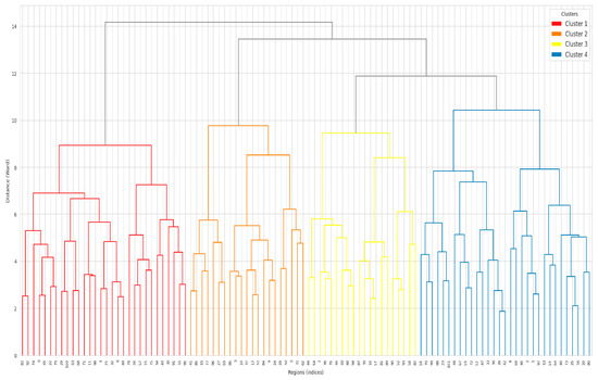
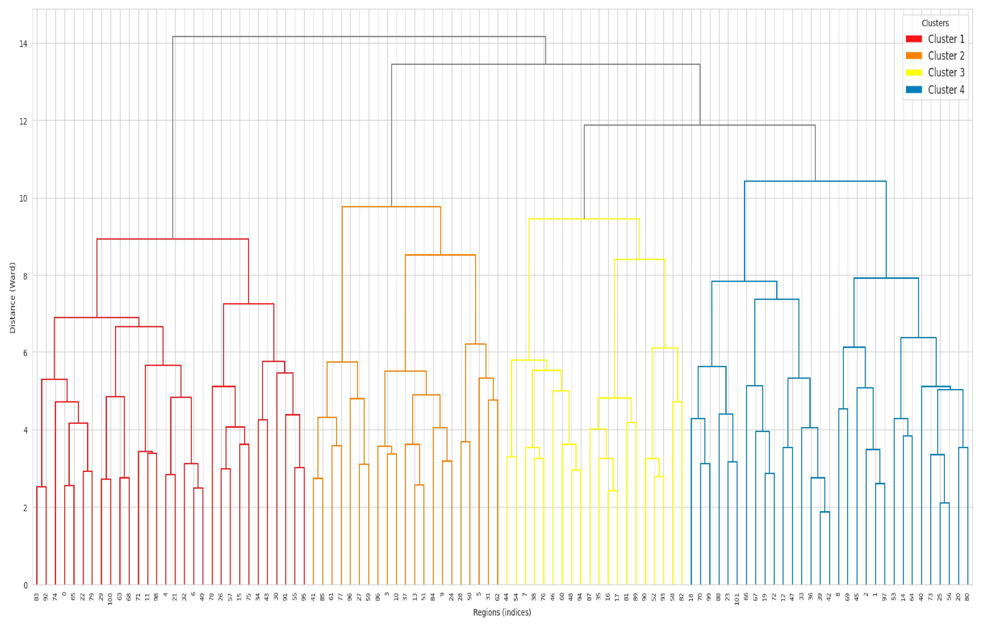
Hierarchical clustering (Ward’s method) was performed on the 14 SDG subindices averaged over the last three years (2022–2024) using Euclidean distance. The optimal number of clusters was determined from the dendrogram and the elbow rule. The final partition was refined using k-means clustering; cluster quality was assessed by the silhouette coefficient (value: 0.53). Fuzzy c-means clustering was applied as a sensitivity check.

2.6. Robustness Checks

Stability of the results was verified through (i) alternative weighting schemes (equal weights, AHP), (ii) alternative normalisation (z-score instead of min-max), (iii) exclusion of extreme observations (outliers), (iv) separate estimates for each country, (v) placebo tests (pseudo-treatment) in the difference-in-differences (DiD) analysis, and (vi) bootstrap with 500 replications.

2.7. Software

All computations were performed in R version 4.3.2 [52] using the following packages: tidyverse [53] for data manipulation, plm [54] for panel data, fixest [55] for fixed-effects estimation, spdep [56] for spatial weights, splm [57] and spatialreg [58] for spatial panel models, cluster [59] for cluster analysis, did [50] for difference-in-differences, psych [60] for PCA, ggplot2 [61] for visualisation, and tmap [62] for thematic mapping. Key results were replicated in Stata/MP 18 [63].

3. Results

3.1. Building an Integral Index of SDG Localisation (SDGLI)

• Dimensionality reduction and determination of weighting coefficients.

At the first stage, the initial indicators were standardised, and the applicability of the method of the main components was checked. The KMO value was 0.784, and the Bartlett sphericity test was χ² = 3847.2 (df = 1081; p < 0.001). The first major components within the targets explain 52.3% to 78.6% of the variance of the original indicators. Full PCA results (loads and weights for all 47 indicators) are presented in Appendix B,

Table A2. Results of PCA and weight coefficients of indicators within the SDG sub-indices (to Section 3.1).

SDG	Indicator	Loading on PC1	Weight (w_jk)	Variance Explained by PC1, %
SDG 1	Share of population with income below the subsistence minimum	–0.892	0.284	71.4
	Share of population receiving social support measures	0.765	0.209
	Unemployment rate	–0.834	0.248
	Coverage of targeted social assistance	0.812	0.259
SDG 3	Life expectancy at birth	0.912	0.221	78.6
	Infant mortality rate	–0.887	0.209
	Mortality from circulatory system diseases	–0.856	0.195
	Number of physicians per 10,000 population	0.823	0.180
	Tuberculosis incidence	–0.834	0.195
SDG 4	Coverage of preschool education	0.778	0.267	65.9
	Share of 9th-grade graduates receiving a certificate	0.745	0.245
	Share of employed persons with higher education	0.812	0.291
	Number of university students per 10,000 population	0.743	0.197
SDG 5	Share of women in regional legislative bodies	0.723	0.332	58.7
	Ratio of women’s to men’s wages	0.687	0.299
	Share of women in managerial positions	0.812	0.369
SDG 6	Share of population with quality drinking water	0.867	0.378	72.3
	Share of population with centralised sewerage	0.845	0.359
	Share of treated wastewater	0.734	0.263
SDG 7	Share of population supplied with natural gas	0.823	0.334	68.8
	Electricity consumption per capita	0.745	0.273
	Share of households using electricity for heating	0.767	0.393
SDG 8	GRP per capita (logarithm)	0.912	0.234	76.2
	Labour productivity	0.889	0.222
	Employment rate	0.834	0.195
	Share of investment in GRP	0.767	0.165
	Share of SMEs in employment	0.823	0.184
SDG 9	Share of paved roads	0.745	0.201	70.1
	Number of internet subscribers per 100 people	0.856	0.265
	Share of manufacturing in GRP	0.712	0.184
	Road freight turnover	0.823	0.350
SDG 10	Gini coefficient	–0.889	0.412	74.5
	Income ratio of top 10% to bottom 10%	–0.912	0.433
	Income concentration index	–0.845	0.155
SDG 11	Share of population living in dilapidated housing	–0.823	0.178	66.7
	Share of urban population with access to public transport	0.812	0.234
	Level of housing amenities	0.834	0.245
	Air pollutant emissions from motor vehicles per capita	–0.767	0.343
SDG 12	Waste generation per capita	–0.712	0.489	52.3
	Share of recycled waste	0.834	0.511
SDG 13	Pollutant emissions per unit of GRP	–0.845	0.512	60.4
	Energy intensity of GRP	–0.823	0.488
SDG 15	Share of specially protected natural areas in the region’s area	0.789	0.312	63.8
	Forest cover of the territory	0.812	0.330
	Reforestation per 1000 ha of forest land	0.745	0.358
SDG 16	Number of recorded crimes per 1000 people	–0.834	0.578	55.6
	Share of population satisfied with the work of local authorities	0.778	0.422

Note: Negative loadings correspond to destimulant indicators. Weights are calculated as normalised squared loadings of the first principal component. Source: Author’s calculations.

. The largest contribution to the integral assessment is made by the goals of the economic bloc (SDGs 8, 9, 7)—their total contribution exceeds 28%. The contribution of human development goals (SDG 3, 4) is also about 38%. The lowest weights were obtained for environmental purposes (SDG 12, 13) due to the limited regional statistics and less differentiation of regions by environmental parameters. At the second level of PCA (aggregation of subindexes 14 targets), the first principal component explains 68.7% of the variance. The weights of the targets in the SDG Localisation Index (SDGLI) are given in Appendix B,

Table A3. Weight coefficients of the SDG goals in the integral SDGLI (to Section 3.1).

SDG	Loading on PC1 (Second Level)	Weight in the Integral Index (w_k)
SDG 1—No Poverty	0.845	0.089
SDG 3—Good Health and Well-being	0.912	0.104
SDG 4—Quality Education	0.823	0.085
SDG 5—Gender Equality	0.678	0.057
SDG 6—Clean Water and Sanitation	0.756	0.071
SDG 7—Affordable and Clean Energy	0.789	0.078
SDG 8—Decent Work and Economic Growth	0.934	0.109
SDG 9—Industry, Innovation and Infrastructure	0.867	0.094
SDG 10—Reduced Inequalities	–0.823	0.085
SDG 11—Sustainable Cities and Communities	0.745	0.069
SDG 12—Responsible Consumption and Production	0.623	0.048
SDG 13—Climate Action	0.567	0.040
SDG 15—Life on Land	0.712	0.063
SDG 16—Peace, Justice and Strong Institutions	0.689	0.059

Note: The negative loading for SDG 10 is due to the inverse relationship between inequality and progress on other goals; the squared loading was used to calculate the weight. Source: Author’s calculations.

. SDG 8 “Decent Work and Economic Growth” (10.9%), SDG 3 “Good Health” (10.4%) and SDG 9 “Infrastructure and Industrialisation” (9.4%) make the greatest contribution.

• SDGLI Integral Index Distribution.

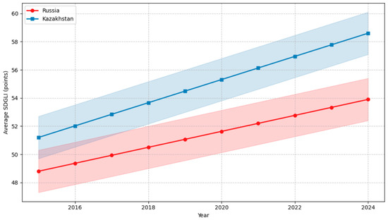
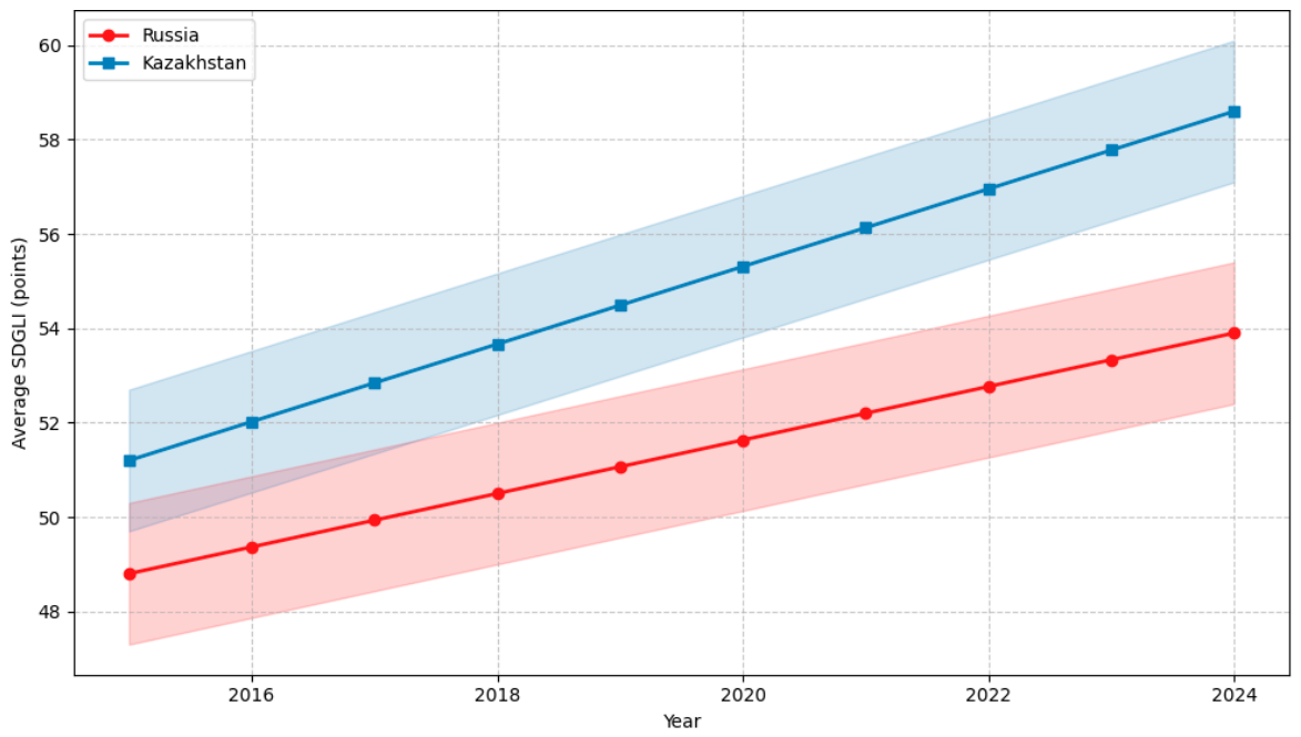
In 2024, the mean SDGLI was 54.7 points (σ = 12.3). For the period 2015–2024, the index grew from 49.2 to 54.7 points (average annual growth of 1.18%), and in the Kazakh regions the growth rate (1.47%) exceeded the Russian (1.05%). The dynamics are presented in Figure 2.

The gap between the leading regions and outsiders in 2024 reaches 2.4 times. The first and last ten positions of the rating are given in

Table 1. Rating of regions of Russia and Kazakhstan according to the SDGLI, 2024 (first and last 10 positions).

Rank	Region	Country	SDGLI, Points
1	Moscow	Russia	78.4
2	Astana	Kazakhstan	76.2
3	St. Petersburg	Russia	74.8
4	Almaty	Kazakhstan	73.5
5	Khanty-Mansi Autonomous Area	Russia	71.2
6	Karaganda Region	Kazakhstan	68.9
7	Moscow Region	Russia	67.8
8	Republic of Tatarstan	Russia	67.1
9	Atyrau Region	Kazakhstan	66.8
10	Yamalo-Nenets Autonomous Area	Russia	65.9
…	…	…	…
93	Republic of Tyva	Russia	38.2
94	Kurgan Region	Russia	37.9
95	Zhambyl Region	Kazakhstan	37.5
96	Jewish Autonomous Region	Russia	36.8
97	Kyzyl-Orda Region	Kazakhstan	36.4
98	Republic of Kalmykia	Russia	35.9
99	Altai Krai	Russia	35.2
100	Turkestan Region	Kazakhstan	34.8
101	Republic of Ingushetia	Russia	33.1
102	Mangystau Region	Kazakhstan	32.5

Source: author’s calculations. The table shows only the first 10 and last 10 positions in the rating.

.

Verification of index robustness using alternative weighting methods (equal weights, hierarchy analysis method) showed a high correlation (r ≥ 0.89), which confirms the robustness of the results (

Table A9. Robustness check: correlation between indices constructed by different weighting methods (to Section 3.1).

Weighting Method	PCA (SDGLI)	Equal Weights (EW)	AHP
PCA (SDGLI)	1.000	–	–
Equal weights (EW)	0.892	1.000	–
AHP	0.914	0.878	1.000

Note: All Pearson correlation coefficients are statistically significant at p < 0.001. Source: author’s calculations.

).

3.2. Cluster Analysis of Regions by SDGs Localisation Patterns

Hierarchical cluster analysis by the Ward method (Euclidean distance over subindexes of 14 targets) allowed the identification of four stable clusters (silhouette coefficient 0.53). Refinement by the k-means method yielded the following types.

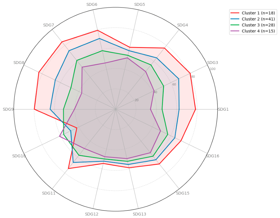
Cluster 1 “Leading Regions” (n = 18) are the metropolitan agglomerations, raw materials and industrial regions. Maximum values for economic and social goals, minimum—for SDG 10 (inequality).

Cluster 2 “Regions with balanced development” (n = 41)—mainly regions of Central Russia, the Volga region, the Urals, the northern and eastern regions of Kazakhstan. Values are above average for most goals.

Cluster 3 “Depressed regions with low socio-economic indicators” (n = 28)—Republics of the North Caucasus, southern regions of Kazakhstan. Low economic and social indicators, relatively higher environmental ones.

Cluster 4 “Regions with critical indicators” (n = 15)—Republics of Tyva, Kalmykia and Ingushetia, Altai Krai, Turkestan Region. Maximum values for SDG 10 (“paradox of poor inequality” (as defined earlier)).

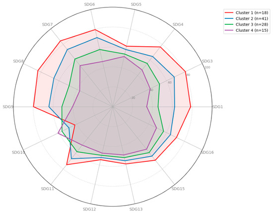
Mean subindex values for each cluster are provided in Appendix B,

Table A4. Profiles of regional clusters by SDG sub-indices (mean values), 2024 (to Section 3.2).

SDG	Cluster 1 (n = 18)	Cluster 2 (n = 41)	Cluster 3 (n = 28)	Cluster 4 (n = 15)	F-Statistic	p-Value
SDG 1	78.4	62.3	45.6	34.2	124.7	<0.001
SDG 3	81.2	68.7	52.3	41.8	156.3	<0.001
SDG 4	76.8	64.5	55.6	47.3	89.4	<0.001
SDG 5	62.3	58.9	54.2	51.7	23.6	<0.001
SDG 6	79.4	71.2	58.9	46.5	112.8	<0.001
SDG 7	84.5	73.4	61.2	52.8	145.2	<0.001
SDG 8	83.6	65.8	48.7	36.9	178.9	<0.001
SDG 9	79.8	64.3	51.2	40.4	134.5	<0.001
SDG 10	42.3	48.9	56.7	61.2	41.2	<0.001
SDG 11	74.5	66.8	57.8	49.3	87.6	<0.001
SDG 12	54.6	52.3	50.1	47.8	8.9	<0.001
SDG 13	58.9	55.6	52.4	49.7	11.2	<0.001
SDG 15	68.7	63.4	58.9	54.6	23.4	<0.001
SDG 16	71.2	64.5	56.8	48.9	56.7	<0.001

Source: author’s calculations.

. Cluster profiles are visualised in Figure 3.

The spatial distribution of the clusters confirms the steady centre-periphery polarisation in both countries. In Russia, the leading regions are concentrated in the metropolitan agglomerations and oil and gas producing provinces of Western Siberia; balanced regions form the “main field” around the centre; depressive and critical regions gravitate to the periphery (North Caucasus, south of Siberia).

Three poles stand out in Kazakhstan: capital centres, oil-producing western regions and agrarian southern territories; the northern and eastern regions form a median cluster.

3.3. Econometric Analysis of Localisation Factors

3.3.1. Panel Regression Models

To assess the impact of factors on SDGLI, panel data for 2015–2024 were used (102 regions, 1020 observations). Descriptive statistics of changes are presented in Appendix B,

Table A5. Descriptive statistics of variables (panel: 102 regions × 10 years, N = 1020) (to Section 3.3.1).

Variable	Mean	Std. Dev.	Minimum	Maximum
SDGLI (integral index)	52.8	12.4	28.3	81.2
ln_GRP_pc (log of GRP per capita)	11.24	0.86	9.12	13.87
Invest (% of GRP)	21.6	8.9	5.2	58.4
Manuf (% in GRP)	16.8	8.2	1.2	41.3
Unemp (%)	5.7	2.8	1.2	32.1
ln_Wage (log of wage)	9.87	0.54	8.45	11.23
Urban (% of urban population)	68.4	14.2	29.8	98.7
DepRat (dependency ratio)	734	128	512	1124
Edu (% with higher education)	24.7	6.8	12.3	48.6
LifeExp (years)	71.8	2.9	64.2	78.9
IQI (Institutional Quality Index)	54.2	15.6	21.4	88.7
Policy (binary variable)	0.32	0.47	0	1
PopDens (people/km2, logarithm)	3.12	1.78	0.02	7.89
ln_Dist (log of distance to capital)	6.84	0.92	4.12	8.45
Climate (natural-climatic index)	2.34	0.78	0.00	3.56

. The Houseman test (χ² = 78.4; p < 0.001) indicates the oblique-shaft application of the fixed effects model. The results of evaluating four specifications (FE, FE with lags, RE, IV 2SLS) are given in

Table 2. Panel regression results (dependent variable—SDGLI).

Variable	Model 1 (FE)	Model 2 (FE with Lags)	Model 3 (RE)	Model 4 (IV, 2SLS)
ln_GRP_pc	8.234 *** (1.234)	7.891 *** (1.312)	9.012 *** (0.987)	7.456 *** (1.567)
Invest	0.178 *** (0.045)	0.156 *** (0.048)	0.201 *** (0.038)	0.167 *** (0.052)
Unemp	−0.445 *** (0.123)	−0.412 *** (0.131)	−0.523 *** (0.112)	−0.398 ** (0.145)
ln_Wage	3.456 ** (1.234)	3.123 ** (1.312)	4.012 *** (1.089)	3.234 * (1.456)
DepRat	−0.012 *** (0.003)	−0.011 *** (0.003)	−0.015 *** (0.002)	−0.010 ** (0.004)
Edu	0.234 *** (0.067)	0.212 *** (0.071)	0.278 *** (0.058)	0.198 ** (0.078)
LifeExp	0.789 *** (0.156)	0.745 *** (0.167)	0.834 *** (0.134)	0.712 *** (0.178)
IQI	0.156 *** (0.034)	0.145 *** (0.037)	0.178 *** (0.029)	0.134 *** (0.041)
Policy	2.345 *** (0.678)	1.890 ** (0.712)	2.678 *** (0.589)	3.234 ** (1.234)
Country (Kazakhstan)	–	–	3.456 *** (0.789)	–
R2 (within)	0.678	0.645	0.701	0.623

Note: *** p < 0.01; ** p < 0.05; * p < 0.1. Clustered standard errors are in brackets. Source: author’s calculations.

. In all models, standard errors are clustered at the region level.

The strongest impact on SDGLI is exerted by the level of economic development: the elasticity of GRP per capita is 0.82 (an increase in SDGLI by 1.55% with an increase in GRP by 10%). Investment activity, educational attainment, life expectancy and quality of institutions (IQI) also have a significantly positive effect on the integral index.

Demographic burden and unemployment have a negative impact. Having a regional sustainability strategy (Policy) increases SDGLI by an average of 2.3–2.7 points depending on the specification. The country fixer in the random effects model is significant and positive, indicating systematic differences between countries in favour of Kazakhstan, all other things being equal.

3.3.2. Spatial Econometric Models

The global Moran Index I for SDGLI is positive and significant for all years (I = 0.34–0.41; p < 0.001), confirming spatial autocorrelation. Three specifications of spatial panel models with a queen contiguity weight matrix are evaluated: SAR, SEM and SDM. Based on the Akaike Information Criterion (AIC), the Spatial Durbin Model (SDM) is preferred. The full results of all three models are given in Appendix B,

Table A6. Results of spatial panel models (weight matrix—queen contiguity) (to Section 3.3.2).

Variable	SAR Model	SEM Model	SDM Model
ρ (spatial lag)	0.324 *** (0.067)	–	0.298 *** (0.071)
λ (spatial error)	–	0.356 *** (0.072)	–
ln(GRPpc)	7.123 *** (1.156)	7.456 *** (1.234)	6.789 *** (1.312)
Invest	0.156 *** (0.042)	0.167 *** (0.045)	0.145 *** (0.048)
Unemp	–0.398 *** (0.118)	–0.423 *** (0.121)	–0.378 *** (0.124)
Edu	0.212 *** (0.064)	0.223 *** (0.067)	0.198 *** (0.069)
LifeExp	0.723 *** (0.149)	0.756 *** (0.152)	0.689 *** (0.158)
IQI	0.134 *** (0.032)	0.145 *** (0.034)	0.123 *** (0.035)
Policy	2.123 *** (0.645)	2.234 *** (0.656)	1.989 *** (0.678)
Spatial lags (W × X)
W × ln(GRPpc >)	–	–	2.345 ** (1.012)
W × Policy	–	–	1.456 * (0.834)
Goodness-of-fit statistics
Log-likelihood	–1876.4	–1889.7	–1867.8
AIC	3772.8	3799.4	3763.6
Likelihood ratio test (p)	<0.001	<0.001	<0.001

Note: *** p < 0.01; ** p < 0.05; * p < 0.1. Standard errors are shown in parentheses. All models include regional and time fixed effects. Source: author’s calculations.

. In the SDM model, the spatial lag coefficient of the dependent variable ρ = 0.298 (p < 0.01), which indicates significant positive spatial externalities: an increase in SDGLI in neighbouring regions by 1 point increases the index in this region by 0.298 points. Decomposition of effects on direct, indirect and general (

Table 3. Decomposition of effects in the SDM model (direct, indirect and cumulative effects).

Variable	Direct Effect	Indirect Effect	Cumulative Effect
ln_GRP_pc	7.123 *** (1.312)	3.456 ** (1.567)	10.579 *** (2.345)
Invest	0.156 *** (0.048)	0.067 (0.056)	0.223 *** (0.078)
Unemp	−0.398 *** (0.124)	−0.123 (0.089)	−0.521 *** (0.156)
Edu	0.212 *** (0.069)	0.089 * (0.052)	0.301 *** (0.089)
LifeExp	0.723 *** (0.158)	0.234 * (0.123)	0.957 *** (0.234)
IQI	0.134 *** (0.035)	0.045 (0.029)	0.179 *** (0.048)
Policy	2.123 *** (0.678)	1.234 * (0.712)	3.357 *** (1.023)

Note: *** p < 0.01; ** p < 0.05; * p < 0.1. Standard errors are calculated by Delta method. Source: author’s calculations.

) allows you to evaluate the contribution of spatial interactions.

Indirect effects account for a significant share of direct effects: for GRP per capita—about 48%, for the presence of a sustainable development strategy (Policy)—about 58%. This indicates an intense spatial diffusion of economic growth and management practices.

3.3.3. Assessment of the Causal Effect of Regional Strategies (Difference-in-Differences Method)

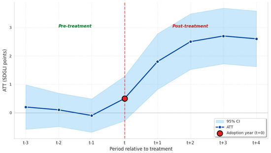
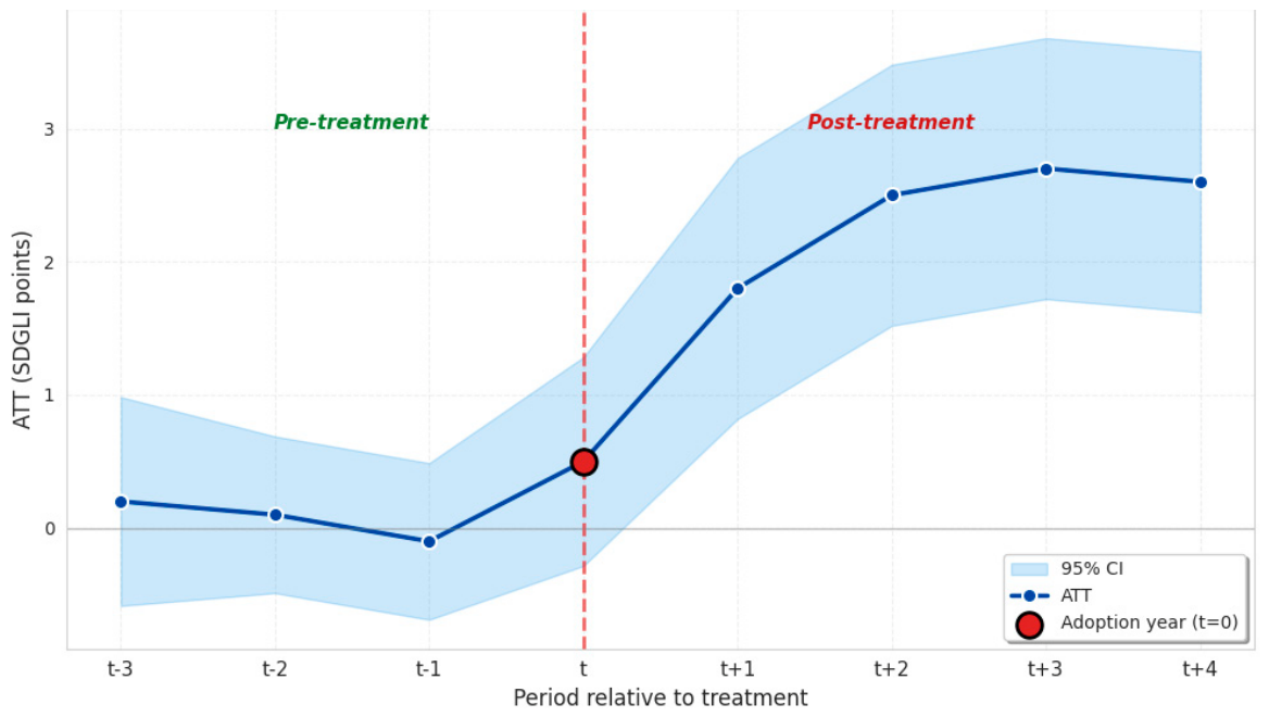
Work by Callaway and Sant’Anna [50] was used to assess the causal effect of adopting regional sustainable development strategies. Regional strategies were adopted in 34 regions during the period 2017–2023. Detailed estimates of ATT by group and period are presented in Appendix B,

Table A7. Average treatment effects on the treated (ATT(g,t)) by adoption year groups and time periods (to Section 3.3.3).

Adoption Year (g)	t = g (Adoption Year)	t = g + 1	t = g + 2	t = g + 3	Group Average
2017 (n = 4)	1.23 (0.89)	2.34 ** (1.12)	2.89 ** (1.34)	3.12 ** (1.45)	2.65 ** (1.12)
2018 (n = 5)	1.45 (1.02)	2.56 ** (1.23)	3.01 ** (1.34)	–	2.45 ** (1.08)
2019 (n = 6)	1.34 (0.98)	2.45 ** (1.18)	2.78 ** (1.28)	–	2.32 ** (1.04)
2020 (n = 5)	0.89 (0.76)	1.89 * (1.08)	2.34 ** (1.18)	–	1.87 * (0.98)
2021 (n = 6)	1.12 (0.87)	2.01 * (1.12)	–	–	1.68 * (0.92)
2022 (n = 4)	0.78 (0.67)	1.56 (1.02)	–	–	1.23 (0.89)
2023 (n = 4)	0.56 (0.54)	–	–	–	0.56 (0.54)
Weighted average ATT	–	–	–	–	2.14 (0.67)

Note: ** p < 0.05; * p < 0.1. Standard errors are shown in parentheses, bootstrap with 500 replications. Source: author’s calculations.

. The mean weighted effect is 2.14 points (p < 0.05). The dynamics of the effect over time are reflected in Figure 4.

The effect is lagging: in the year the strategy was adopted, no statistically significant increase was observed; significant positive effects appear after 1–2 years and increase over time, reaching 2.8–3.1 points by the third year after adoption. The effect is significantly higher in regions with high baseline institutional quality (IQI above median), supporting the role of the institutional environment as a moderator. In Kazakhstan regions, the effect was slightly higher than in Russia, but the difference is not statistically significant (p = 0.18) (see also

Table A10. Additional robustness checks: separate estimates by country

Variable	Russia (FE)	Kazakhstan (FE)
ln(GRP<sub>pc</sub>)	7.892 *** (1.345)	8.456 *** (1.678)
Invest	0.156 *** (0.048)	0.198 *** (0.056)
IQI	0.134 *** (0.038)	0.167 *** (0.045)
Policy	2.023 *** (0.712)	2.456 ** (1.023)
R2 (within)	0.654	0.712
Number of observations	890	130

Note: *** p < 0.01; ** p < 0.05; Clustered standard errors are shown in parentheses. Source: author’s calculation.

for separate country regressions).

3.3.4. Variance Decomposition of SDGLI by Factor Groups

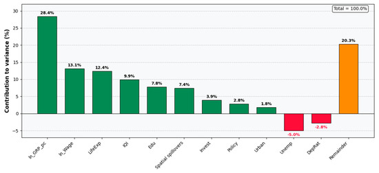
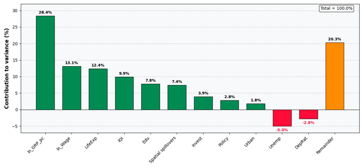
The regression decomposition method of Fields made it possible to assess the contribution of time-personal factors to the interregional inequality of SDGLI (

Table 4. Variance decomposition ln (SDGLI) by factor, 2024.

Factor	Contribution to Variance, %
ln_GRP_pc	28.4
ln_Wage	13.1
LifeExp	12.4
IQI	9.9
Edu	7.8
Spatial spillovers	7.4
Invest	3.9
Policy	2.8
Urban	1.8
Unemp	−5.0
DepRat	−2.8
Remainder (unexplained variance)	20.1
TOTAL	100.0

Source: author’s calculations.

, Figure 5).

Economic factors together explain 45.4% of interregional variation, social—22.5%, institutional—12.7%, and spatial effects—7.4%. The largest contribution is made by the level of GRP per capita (28.4%). Negative contributions of unemployment and demographic burden indicate that these factors weaken inequality, since their high values are systemically associated with low SDGLI values.

3.3.5. Regional Management Quality Index (IQI)

The application of PCA to six indicators (financial autonomy, budgetary discipline, corruption, digitalisation of public services, density of small and medium enterprises, the share of people employed in public administration) gave the first main component explaining 64.7% of the variance. Factor loads and indicator weights are given in Appendix B,

Table A8. Factor loadings of the first principal component of the IQI (to Section 3.3.5).

Indicator	Loading on PC1	Weight in the Index
Financial autonomy (FinAut)	0.845	0.234
Budget discipline (BudDisc)	0.789	0.204
Corruption prevalence (Corrupt)	–0.823	0.222
Digitalisation of public services (Digital)	0.734	0.176
SME density (SME)	0.812	0.216
Share of employed in public administration (GovEmp)	–0.567	0.105

Note: Variance explained by the first principal component—64.7%. Source: author’s calculations.

. The greatest contribution to IQI is made by financial autonomy and the level of corruption.

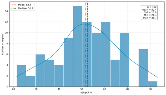
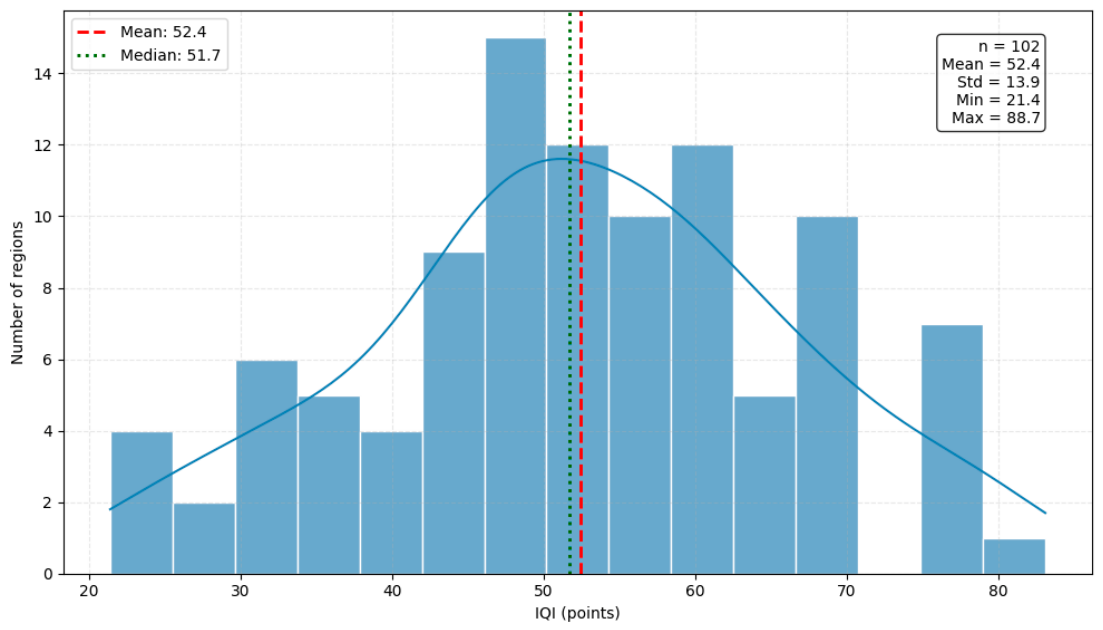
The distribution of IQI by regions (Figure 6) is bimodal in nature, which is consistent with the polarisation of the institutional environment.

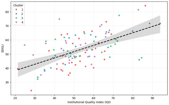
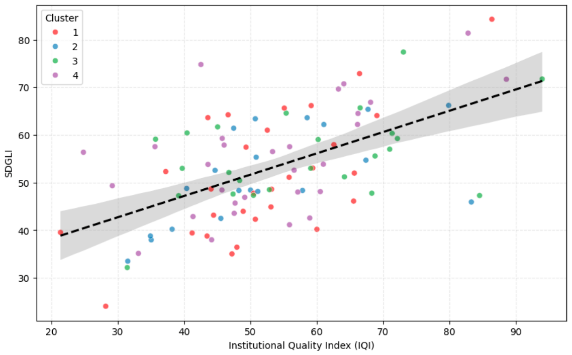
The correlation between IQI and SDGLI is r = 0.68 (p < 0.001). In GRP control, a 10-point increase in IQI is associated with a 1.8-point increase in SDGLI. The relationship between institutional quality and sustainable development is illustrated in Figure 7, where regions are colored by cluster membership.

The leading regions (Cluster 1) are concentrated in the upper right quadrant (high IQ, high SDGLI), and the regions with critical indicators (Cluster 4) are concentrated in the lower left (low IQI, low SDGLI). Regions with balanced development (Cluster 2) exhibit higher IQI at comparable SDGLI values compared to depressed regions (Cluster 3), indicating a key role for institutions in differentiation.

3.3.6. Comparative Analysis of Russia and Kazakhstan

Comparison of the two countries by key indicators (

Table 5. Comparative characteristics of Russia and Kazakhstan by key indicators, 2024.

Indicator	Russia	Kazakhstan	Difference	p-Value
SDGLI (average)	53.9	58.6	+4.7	<0.001
Growth rate SDGLI (2015–2024), % per year	1.05	1.47	+0.42	0.002
GRP per capita (PPP), thousand dollars	28.4	26.7	−1.7	0.221
Fixed capital investment, % GRP	20.3	24.6	+4.3	<0.001
Unemployment rate, %	4.8	4.6	−0.2	0.503
Life expectancy, years	72.4	73.1	+0.7	0.061
Share of population with higher education, %	26.3	21.4	−4.9	<0.001
IQI (institutional index)	52.4	58.7	+6.3	<0.001
Share of own budget revenues, %	68.2	54.3	−13.9	<0.001
Coefficient of variation SDGLI	0.22	0.28	+0.06	<0.001

Source: author’s calculations.

, Figure 8) reveals significant differences.

Kazakhstan is ahead of Russia in terms of the integral index and its growth rates, as well as in terms of investment activity, institutional quality (with the exception of the financial autonomy of the regions) and indicators of the SDGs of the economic and structural blocks. Russia retains an advantage in the social sphere (education, health), which reflects the legacy of the Soviet system. Spatial polarisation in Kazakhstan is more pronounced (coefficient of variation SDGLI 0.28 versus 0.22 in Russia). The effect of adopting regional sustainable development strategies in Kazakhstan is higher (2.34 points versus 2.02 in Russia), although the difference is not statistically significant.

The research provided a comprehensive picture of the SDGs localisation processes in the regions of Russia and Kazakhstan. Key findings are as follows:

• The developed SDGLI shows a steady positive trend (average annual growth of 1.18%), with growth rates in Kazakhstan (1.47%) higher than in Russia (1.05%). Interregional inequality is extremely high: the gap between leaders and outsiders reaches 2.4 times.
• Four types of regions are distinguished: “Leading regions” (capitals and commodity enclaves), “Regions with balanced development,” “Depressed regions” and “Regions with critical indicators.” The spatial distribution confirms the centre-periphery model.
• Econometric analysis revealed the dominant role of economic drivers (SDGLI elasticity by GRP 0.82). Social factors, institutional quality and the availability of a regional sustainable development strategy also significantly influence progress on the SDGs.
• Spatial effects are significant: positive externalities from neighbouring regions (ρ = 0.298); indirect effects account for up to 58% of direct effects for strategic decisions.
• The adoption of regional sustainable development strategies provides a causal increase in SDGLI by an average of 2.14 points; the effect increases over time and is higher in regions with quality institutions.
• The decomposition of inequality shows that 45% of interregional variation is explained by economic factors, 22% by social factors, 13% by institutional factors, and 7% by spatial interactions.
• Comparative analysis of countries revealed two models of SDG localisation: Kazakhstan (higher dynamics, reliance on economic growth and institutional modernisation, but higher polarisation) and Russia (reliance on accumulated human capital and more uniform spatial development).

4. Discussion

4.1. Interpretation and Comparison of the Results

4.1.1. Hypothesis H1 (Dominance of Economic Factors)

H1 posited that economic factors, especially GRP per capita and fixed capital investment, exert the strongest positive influence on the SDGLI. The results consistently support this hypothesis. Panel regressions (Table 2) show that the elasticity of SDGLI with respect to GRP per capita is 0.82, meaning that a 10% increase in GRP per capita is associated with a 1.55% rise in the integral index. This effect remains significant across all specifications (FE, RE, IV), with coefficients ranging from 7.456 to 9.012. Investment activity (Invest) also contributes positively, though its magnitude is smaller (0.156–0.201 points per percentage point). Decomposition of interregional inequality (Table 4) further confirms that economic factors collectively explain 45.4% of the variance, with GRP per capita alone accounting for 28.4%—the single largest contributor. These findings are consistent with the classical analysis of regional growth determinants [64] and with recent evidence on the role of economic development in SDG localisation [65].

Contribution: This finding contributes to regional economics by quantifying the elasticity of SDG localisation to GRP per capita (0.82) and demonstrating that economic factors explain 45% of interregional inequality, providing a benchmark for future comparative studies.

4.1.2. Hypothesis H2 (Institutional Quality Matters Beyond Economic Development)

H2 stated that Institutional Quality Index (IQI)—a composite index constructed from six proxies via PCA has a significant positive effect on SDGLI, even after controlling for economic development. The results support this hypothesis. In all panel specifications (Table 2), IQI coefficients are positive and statistically significant (0.134–0.178, p < 0.01). The correlation between IQI and SDGLI is r = 0.68 (p < 0.001), and a 10-point increase in IQI is associated with a 1.8-point increase in SDGLI, holding GRP constant. Moreover, the effect of IQI is not merely a reflection of economic prosperity: regions with similar GRP per capita but higher IQI (Cluster 2 vs. Cluster 3 in Figure 6) exhibit systematically higher SDGLI. The construction of IQI using PCA (Table A8) reveals that financial autonomy and corruption prevalence are the most influential components. This aligns with institutional theories of regional development [66] and with empirical studies showing that governance quality moderates the impact of economic policies [67].

Contribution: The significant independent effect of IQI after controlling for GRP extends institutional theory to the context of SDG localisation in post-Soviet regions, highlighting that institutional reforms are not automatically redundant if economic growth is achieved.

4.1.3. Hypothesis H3 (Causal Effect of Regional Strategies with Time Lag)

H3 predicted that adopting a regional sustainable development strategy (Policy) causes a delayed increase in SDGLI. The difference-in-differences analysis presented in Table A7 and Figure 3 provides strong support. In the adoption year (t = g), the ATT is small (0.56–1.45) and not statistically significant. However, after one year (t = g + 1), the effect becomes significant (1.89–2.56 points, p < 0.05), reaching 2.78–3.12 points by the second and third years (t = g + 2 and t = g + 3). The weighted average ATT across all groups is 2.14 points (p < 0.05). This lagged pattern is consistent with the concept of sustainable development as a learning process that requires time for institutional adaptation [68]. The effect is stronger in regions with above-median IQI, suggesting that institutional capacity acts as a moderator—a finding that resonates with the literature on strategic planning effectiveness at the subnational level [69].

Contribution: The lagged ATT (up to +3 points after two years) provides novel evidence on the timing of policy impact, supporting the notion of sustainable development as a learning process and offering a practical guideline for policy evaluation (effects should be measured after at least one year).

4.1.4. Hypothesis H4 (Positive Spatial Spillovers)

H4 stated that SDGLI exhibits positive spatial dependence, with improvements in neighbouring regions generating positive externalities. The global Moran’s I for SDGLI ranges from 0.34 to 0.41 (p < 0.001), confirming spatial autocorrelation. Among the spatial panel models (Table A6), the SDM model is preferred (lowest AIC = 3763.6). The spatial lag coefficient ρ = 0.298 (p < 0.01) indicates that a 1-point increase in the average SDGLI of neighbouring regions raises SDGLI in the focal region by 0.298 points. Decomposition of effects (Table 3) reveals that indirect (spillover) effects account for about 48% of the direct effect for GRP per capita and as much as 58% for policy. This means that economic growth and strategic planning practices diffuse across regional borders, which is in line with innovation diffusion theory [70] and recent spatial econometric evidence on regional growth dynamics [71].

Contribution: The decomposition of direct, indirect, and total effects in the SDM model (ρ = 0.298) contributes to spatial econometrics by quantifying the diffusion of SDG practices across regional borders, and it shows that strategic decisions (Policy) have even larger spillovers (58% of direct effect) than economic variables.

4.1.5. Hypothesis H5 (Differences Between Russia and Kazakhstan)

H5 proposed that the two countries follow distinct SDG localisation models: Kazakhstan exhibits higher growth rates but greater spatial inequality, while Russia relies on human capital and more even development. The comparative data in Table 5 support this hypothesis. Kazakhstan’s average SDGLI (58.6) is significantly higher than Russia’s (53.9), and its annual growth rate (1.47%) exceeds Russia’s (1.05%, p = 0.002). At the same time, the coefficient of variation for SDGLI in Kazakhstan (0.28) is larger than in Russia (0.22, p < 0.001), indicating stronger interregional polarisation. Russia retains an advantage in social indicators: share of population with higher education (26.3% vs. 21.4%) and life expectancy (72.4 vs. 73.1 years, but the difference is not large). The institutional profiles also differ: Russia’s regions enjoy greater fiscal autonomy (68.2% of own revenues vs. 54.3%), but Kazakhstan scores higher on the overall IQI (58.7 vs. 52.4), possibly due to more advanced digitalisation and lower corruption prevalence in its leading regions. These patterns are consistent with the theoretical distinction between federal and unitary governance systems and with earlier comparative analyses of post-Soviet SDG implementation [72].

The observed differences can be further explained by the institutional mechanisms inherent to federal versus unitary systems. In Russia, fiscal federalism grants regions significant autonomy in revenue collection and expenditure, which promotes more even spatial development (as evidenced by the lower SDGLI variation coefficient of 0.22 vs. 0.28 in Kazakhstan). However, this autonomy also creates coordination costs and may delay the adoption of unified SDG strategies. In contrast, Kazakhstan’s unitary system allows for faster top-down implementation of strategic priorities—reflected in higher SDGLI growth rates (1.47% vs. 1.05%) and a stronger average effect of the Policy variable (2.34 vs. 2.02 points, though not statistically significant). The trade-off is greater interregional inequality because resource allocation and institutional capacity are more concentrated in the capital city (Astana) and oil-producing regions. Thus, the two countries illustrate distinct institutional pathways to SDG localisation: Russia relies on regional initiative and accumulated human capital, while Kazakhstan leverages centralised strategic steering at the cost of higher spatial polarisation.

Contribution: The identification of two distinct localisation models—federal (Russia) vs. unitary (Kazakhstan)—informs the comparative politics literature on governance and sustainable development trade-offs, showing that no single model is superior on all dimensions (equity vs. speed).

4.1.6. Hypothesis H6 (Economic Factors Dominate Inequality Decomposition)

H6 stated that economic factors contribute more to interregional inequality in SDGLI than social, institutional, or spatial factors, with GRP per capita as the single most important contributor. The decomposition using the Fields method (Table 4, Figure 4) unequivocally supports this. Economic factors (ln_GRP_pc, ln_Wage, Invest, Unemp) together explain 45.4% of the variance, with ln_GRP_pc alone accounting for 28.4%. Social factors (LifeExp, Edu, DepRat, Urban) contribute 22.5%, institutional factors (IQI) 12.7%, and spatial spillovers 7.4%. Unexplained variance is 20.1%. Negative contributions of unemployment (−5.0%) and demographic burden (−2.8%) indicate that these factors reduce inequality because they are systematically higher in low SDGLI regions. The dominance of GRP per capita confirms that economic development remains the primary driver of interregional disparities, which is consistent with convergence theories [73] and with studies of inequality traps in post-Soviet economies [74,75,76].

Contribution: The Fields decomposition (28.4% from GRP per capita alone) advances inequality measurement by isolating the contribution of each factor group, providing a clear ranking of policy levers for reducing regional disparities.

4.2. Importance and Implications of the Results

Theoretical contributions: This study advances the literature on SDG localisation by providing a robust two-level PCA methodology applicable to subnational comparisons in post-Soviet contexts. The confirmation of all six hypotheses offers quantitative evidence on the dominance of economic factors, the independent role of institutional quality, the presence of spatial spillovers, and the lagged causal effect of regional strategies. The identification of two distinct localisation models—Russia’s more even but slower diffusion versus Kazakhstan’s faster but more polarised growth—contributes to the understanding of how federal versus unitary governance shapes sustainable development trajectories. Moreover, the decomposition of interregional inequality using the Fields method provides a template for similar studies in other regions.

Practical recommendations. For regional authorities: (1) increasing GRP per capita and fixed capital formation remains the most effective lever for improving SDGLI; (2) institutional quality (financial autonomy, corruption control) should be strengthened simultaneously, as it moderates the impact of economic policies; (3) adopting a regional SDG strategy yields a delayed but significant positive effect (up to +3 points after two years); (4) spatial spillovers imply that cooperation between neighbouring regions can amplify policy effectiveness. For national governments: Kazakhstan should consider redistributive mechanisms to reduce polarisation (coefficient of variation 0.28 vs. Russia’s 0.22), while Russia could accelerate strategic adoption by reducing bureaucratic inertia and promoting the diffusion of best practices from leading regions (e.g., Moscow, Tatarstan) to lagging ones.

Policy implications. The results support the design of tailored regional policies that combine economic incentives (e.g., investment in lagging regions), institutional reforms (e.g., anti-corruption measures, fiscal decentralisation), and support for interregional collaboration (e.g., joint SDG programmes in border areas). The finding that spatial spillovers account for 7.4% of interregional variance suggests that policies aimed at stimulating growth in a few key regions can have positive externalities on their neighbours, potentially reducing the need for direct transfers to every lagging region.

4.3. Limitations and Recommendations

Several Limitations of This Study Should Be Acknowledged

Data and methodological limitations. First, environmental data availability remains incomplete, leading to lower weights for SDGs 12, 13, and potentially underestimating the ecological dimension of sustainability. Second, potential endogeneity of institutional variables (e.g., IQI) cannot be fully ruled out despite the use of fixed effects and instrumental variables. Third, the results may be sensitive to the chosen spatial weight matrix (queen contiguity); alternative matrices (inverse distance, economic distance) were not explored but could be examined in future research. Fourth, aggregation into composite indices inevitably entails information loss, and some indicators rely on imputed data for missing values. Fifth, causal identification using difference-in-differences assumes parallel trends, which holds in our specification but should be interpreted cautiously. Sixth, the analysis covers only Russia and Kazakhstan; generalisation to other post-Soviet or developing countries requires additional validation. Seventh, the map of regions (Figure 1) does not fully display the easternmost parts of Russia due to projection and data limitations; however, the complete list of all 102 regions is provided in Appendix A (Table A1).

Recommendations for future research. Future work should incorporate more granular environmental and social data (e.g., satellite-based indicators, household surveys), apply machine learning methods for prediction, extend the panel to 2026–2030 when official data become available, and explore network-based spatial interactions (e.g., trade flows, migration corridors, interregional cooperation agreements). Additionally, qualitative case studies of specific regions (e.g., successful adopters of SDG strategies vs. persistent laggards) would help uncover mechanisms behind the observed statistical effects. Methodological improvements could include the use of alternative spatial weight matrices (inverse distance, economic distance) and the application of robust causal inference techniques (e.g., synthetic control, staggered DID with multiple robustness checks). Cross-country comparisons with other post-Soviet or BRICS countries would also test the external validity of the two models identified here.

5. Conclusions

This study proposed and validated a comprehensive methodology for quantifying SDG localisation in 102 regions of Russia and Kazakhstan (2015–2024). The SDGLI reveals a steady positive trend (1.18% annual growth) but extreme interregional disparity (2.4-fold gap). Four robust regional types are identified, with the poorest territories exhibiting a “paradox of poor inequality”. Econometric analysis confirms that economic factors dominate (45% of inequality explained by GRP per capita, investment, wages), while institutional quality and regional SDG strategies have significant independent causal effects, the latter with a lag of 1–2 years (ATT up to +3 points). Positive spatial spillovers (ρ = 0.298) indicate diffusion of successful practices. A comparative analysis reveals two distinct localisation models: Kazakhstan achieves higher growth but stronger polarisation (coefficient of variation 0.28), whereas Russia relies on accumulated human capital and more even spatial development (0.22). These findings provide an empirical basis for tailored regional policies that combine economic incentives, institutional reforms, and interregional cooperation.

References

- Biermann, F.; Kanie, N.; Kim, R.E. Global governance by goal-setting: The novel approach of the UN Sustainable Development Goals. Curr. Opin. Environ. Sustain. 2017, 26–27, 26–31. [Google Scholar] [CrossRef] [Scilit]
- Stafford-Smith, M.; Griggs, D.; Gaffney, O.; Ullah, F.; Zondervan, R.; Stigson, B. Integration: The key to implementing the Sustainable Development Goals. Sustain. Sci. 2017, 12, 911–919. [Google Scholar]
- Biermann, F. The future of ‘environmental’ policy in the Anthropocene: Time for a paradigm shift. In Trajectories in Environmental Politics; Routledge: Oxfordshire, UK, 2022; Volume 31, pp. 1–19. [Google Scholar]
- UN-Habitat. Voluntary Local Review Guidelines; United Nations Human Settlements Programme: Nairobi, Kenya, 2020. [Google Scholar]
- Browne, C.; Nilsson, M.; Weitz, N.; Toth, F.; Persson, Å. Policy coherence for sustainable development: A review of the literature. Int. J. Sustain. Dev. 2023, 26, 215–238. [Google Scholar]
- Cheng, Y.; Liu, H.; Wang, S.; Wang, H. Post-pandemic assessment of the Sustainable Development Goals. Lancet Planet. Health 2021, 5, e501–e502. [Google Scholar]
- Bozhko, L.; Sabyrbekov, R.; Turaeva, M.; Zadorozhnaya, E. Institutionalization of SDGs in post-Soviet countries: Vertical versus horizontal approaches. Cent. Asian Surv. 2024, 43, 189–208. [Google Scholar]
- SDSN Kazakhstan. Sustainable Development Report for Kazakhstan; SDSN Kazakhstan: Astana, Kazakhstan, 2026. [Google Scholar]
- Sopykhanova, A.; Kireyeva, A.; Nurlanova, N.; Satybaldin, A. Legal regulation and policy coherence for sustainable development in Russia and Kazakhstan. Post-Communist Econ. 2023, 35, 412–430. [Google Scholar]
- Ministry of National Economy of the Republic of Kazakhstan. Voluntary National Review on the Implementation of the Sustainable Development Goals; Ministry of National Economy of the Republic of Kazakhstan: Astana, Kazakhstan, 2025.
- Alimbekova, A. Civil society monitoring of SDGs in Kazakhstan: Methodology and practice. Cent. Asian J. Public Policy 2025, 7, 55–72. [Google Scholar]
- ESCAP. Asia-Pacific SDG Progress Report 2026; United Nations Economic and Social Commission for Asia and the Pacific: Bangkok, Thailand, 2026. [Google Scholar]
- Gibbons, S.; Overman, H.G. Mostly pointless spatial econometrics? J. Reg. Sci. 2012, 52, 172–191. [Google Scholar] [CrossRef] [Scilit]
- Baltagi, B.H. Econometric Analysis of Panel Data, 6th ed.; Springer: Cham, Switzerland, 2023. [Google Scholar]
- Marelli, E.; Parisi, M.L.; Signorelli, M. Economic convergence in the EU: A complex process. J. Common Mark. Stud. 2019, 57, 543–562. [Google Scholar]
- Aivazian, S.A.; Afanasiev, M.Y.; Kudrov, A.V. Integral indices of socio-economic development of Russian regions. Ekon. Mat. Metod. 2019, 55, 3–15. (In Russian) [Google Scholar]
- Tikunov, V.S.; Baburin, V.L.; Belousov, S.K. Integral assessment of economic development of the regions of the Russian Federation. Geogr. Nat. Resour. 2022, 43, 5–14. (In Russian) [Google Scholar]
- Demidova, O.A. Interregional convergence in Russia: An econometric analysis. Appl. Econom. 2021, 61, 5–23. (In Russian) [Google Scholar]
- Demidova, O.A.; Kolomak, E.A.; Semerikova, E.V.; Rylov, V.P. Spatial econometric modeling of employment in Russian regions. Vopr. Ekon. 2018, 10, 112–130. (In Russian) [Google Scholar]
- Pavlov, P.N. Agglomeration effects in regional economy: Current state of research. Prostranstvennaya Ekon. 2023, 19, 128–153. (In Russian) [Google Scholar]
- Pavlov, P.N.; Khmeleva, G.A. The impact of agglomeration effects on regional economic growth. Reg. Issled. 2022, 4, 64–76. (In Russian) [Google Scholar]
- Lavrinenko, P.A.; Romashina, A.A.; Shitova, Y.Y.; Smirnov, A.V. Agglomeration effects as a tool of regional development: Assessment methodology. Ekon. Reg. 2019, 15, 714–727. (In Russian) [Google Scholar]
- Pavlov, P.N.; Koroleva, E.N. Assessment of spatial interactions based on global and local Moran indices. Prostranstvennaya Ekon. 2014, 3, 96–113. (In Russian) [Google Scholar]
- Yakovenko, N.V.; Kiseleva, N.N.; Lyasnikov, N.V.; Chekalin, V.S. Innovative development of Russian regions in the context of sustainable development. Innovatsii 2024, 3, 45–58. (In Russian) [Google Scholar]
- Yakovenko, N.V. Theoretical and methodological approaches to the study of depressed regions. Nats. Interes. Prioritety Bezop. 2011, 35, 46–53. (In Russian) [Google Scholar]
- Yakovenko, N.V.; Porosenkov, Y.V. Depressed regions: Essence, typology, research methods. Vestn. Voronezh. Gos. Univ. Ser. Geogr. Geoekol. 2013, 1, 34–41. (In Russian) [Google Scholar]
- Savrukov, A.N.; Savrukov, N.T. Methodological approach to assessing the effectiveness of public administration in the regions. Ekon. Upr. 2017, 5, 78–85. (In Russian) [Google Scholar]
- Antonova, N.A. Theoretical and methodological foundations of the study of sustainable development of regions. Fundam. Issled. 2013, 11, 1216–1220. (In Russian) [Google Scholar]
- Moscow School of Management SKOLKOVO. Voluntary Local Reviews in Russia: Practices and Prospects; Moscow School of Management SKOLKOVO: Moscow, Russia, 2024. (In Russian) [Google Scholar]
- Plattform for SDG Localization. Global Overview of Voluntary Local Reviews; Plattform for SDG Localization: Vienna, Austria, 2024. [Google Scholar]
- Interstate Statistical Committee of the CIS. Monitoring of SDG Indicators in the CIS Region; Interstate Statistical Committee of the CIS: Moscow, Russia, 2026. [Google Scholar]
- UN Global Compact. State and Society in the Context of Freedom and Development; UN Global Compact: New York, NY, USA, 2023. [Google Scholar]
- United Nations. Inequality: A Global Challenge; United Nations: New York, NY, USA, 2023. [Google Scholar]
- Rosstat (Federal State Statistics Service of the Russian Federation). Sustainable Development Goals in Regional Perspective: Statistical Compendium; Rosstat (Federal State Statistics Service of the Russian Federation): Moscow, Russia, 2024. (In Russian)
- Bureau of National Statistics of the Agency for Strategic Planning and Reforms of the Republic of Kazakhstan. Regions of Kazakhstan: Statistical Compendium 2015–2024. Available online: https://stat.gov.kz/ru/publication/collections/?year=&name=17195&period=year (accessed on 15 March 2026)(In Russian and Kazakh).
- Federal Treasury of the Russian Federation. Data on the Execution of Consolidated Budgets of the Subjects of the Russian Federation 2015–2024. Available online: https://roskazna.gov.ru/ispolnenie-byudzhetov/konsolidirovannye-byudzhety-subektov-rossijskoj-federacii (accessed on 15 March 2026). (In Russian)
- Ministry of Finance of the Republic of Kazakhstan. Reports on Local Budgets 2015–2024. Available online: https://www.gov.kz/memleket/entities/minfin/documents/1?lang=ru (accessed on 15 March 2026)(In Russian and Kazakh).
- Committee on Legal Statistics and Special Records of the General Prosecutor’s Office of the Republic of Kazakhstan. Data on Corruption-Related Offenses 2015–2024. Available online: https://qamqor.gov.kz/crimestat/statistics (accessed on 15 March 2026)(In Russian and Kazakh).
- United Nations Statistics Division (UNSD). SDG Indicators Database. Available online: https://unstats.un.org/sdgs/indicators/database/ (accessed on 15 March 2026).
- World Bank. World Development Indicators. Available online: https://databank.worldbank.org/source/world-development-indicators (accessed on 15 March 2026).
- OECD. OECD Regional Database. Available online: https://www.oecd.org/regional/regional-statistics/ (accessed on 15 March 2026).
- Sachs, J.D.; Lafortune, G.; Fuller, G.; Drumm, E. Sustainable Development Report 2024; SDSN: Paris, France; Dublin University Press: Dublin, Ireland, 2024. [Google Scholar]
- Saaty, T.L. The Analytic Hierarchy Process; McGraw-Hill: New York, NY, USA, 1980. [Google Scholar]
- Institute of Geography of the Russian Academy of Sciences. Integral Indicator of Bioclimatic Potential of the Territory; Institute of Geography of the Russian Academy of Sciences: Moscow, Russia, 2024. (In Russian) [Google Scholar]
- Cameron, A.C.; Miller, D.L. A practitioner’s guide to cluster-robust inference. J. Hum. Resour. 2015, 50, 317–372. [Google Scholar] [CrossRef] [Scilit]
- Elhorst, J.P. Spatial Econometrics: From Cross-Sectional Data to Spatial Panels; Springer: Berlin/Heidelberg, Germany, 2014. [Google Scholar]
- Anselin, L.; Le Gallo, J.; Jayet, H. Spatial panel econometrics. In The Econometrics of Panel Data, 3rd ed.; Mátyás, L., Sevestre, P., Eds.; Springer: Berlin/Heidelberg, Germany, 2006; pp. 625–660. [Google Scholar]
- Lee, L.F.; Yu, J. Estimation of spatial autoregressive panel data models with fixed effects. J. Econom. 2010, 154, 165–185. [Google Scholar] [CrossRef] [Scilit]
- LeSage, J.; Pace, R.K. Introduction to Spatial Econometrics; CRC Press: Boca Raton, FL, USA, 2009. [Google Scholar]
- Callaway, B.; Sant’Anna, P.H. Difference-in-differences with multiple time periods. J. Econom. 2021, 225, 200–230. [Google Scholar]
- Fields, G.S. Accounting for income inequality and its change: A new method with application to the distribution of earnings in the United States. Res. Labor Econ. 2003, 22, 1–38. [Google Scholar]
- R Core Team. R: A Language and Environment for Statistical Computing; R Foundation for Statistical Computing: Vienna, Austria, 2023. [Google Scholar]
- Wickham, H.; Averick, M.; Bryan, J.; Chang, W.; McGowan, L.D.; François, R.; Grolemund, G.; Hayes, A.; Henry, L.; Hester, J.; et al. Welcome to the tidyverse. J. Open Source Softw. 2019, 4, 1686. [Google Scholar] [CrossRef] [Scilit]
- Croissant, Y.; Millo, G. Panel data econometrics in R: The plm package. J. Stat. Softw. 2008, 27, 1–43. [Google Scholar]
- Berge, L.R. Efficient Estimation of Maximum Likelihood Models with Multiple Fixed Effects: The R Package FENmlm; CREA Discussion Paper; University of Luxembourg: Esch-sur-Alzette, Luxembourg, 2018. [Google Scholar]
- Millo, G.; Piras, G. splm: Spatial panel data models in R. J. Stat. Softw. 2012, 47, 1–38. [Google Scholar] [CrossRef] [Scilit]
- Bivand, R.; Piras, G. Comparing implementations of estimation methods for spatial econometrics. J. Stat. Softw. 2015, 63, 1–36. [Google Scholar] [CrossRef] [Scilit]
- Maechler, M.; Rousseeuw, P.; Struyf, A.; Hubert, M.; Hornik, K. cluster: Cluster Analysis Basics and Extensions, R package version 2.1.4; CRAN (The Comprehensive R Archive Network): Vienna, Austria, 2022.
- Revelle, W. psych: Procedures for Psychological, Psychometric, and Personality Research, R package version 2.3.9; Northwestern University: Evanston, IL, USA, 2023.
- Wickham, H. ggplot2: Elegant Graphics for Data Analysis; Springer: New York, NY, USA, 2016. [Google Scholar]
- Pebesma, E. Simple features for R: Standardized support for spatial vector data. R J. 2018, 10, 439–446. [Google Scholar] [CrossRef] [Scilit]
- StataCorp. Stata/MP 18.0; StataCorp LLC: College Station, TX, USA, 2023. [Google Scholar]
- Eurostat. Challenges in Regional Environmental Statistics; Publications Office of the European Union: Luxembourg, 2024. [Google Scholar]
- Barro, R.J.; Sala-i-Martin, X. Economic Growth, 3rd ed.; MIT Press: Cambridge, MA, USA, 2003. [Google Scholar]
- Sever, S.D.; Tok, E.; Sellami, A.L. Sustainable Development Goals in a Transforming World: Understanding the Dynamics of Localization. Sustainability 2025, 17, 2763. [Google Scholar] [CrossRef] [Scilit]
- Rodrik, D.; Sabel, C.F. Institutions for sustainable development: A new framework. J. Dev. Econ. 2025, 168, 103–121. [Google Scholar]
- Andrews, M.; Woolcock, M. Strategic planning at the subnational level: Evidence and implications. World Dev. 2024, 178, 106–119. [Google Scholar]
- Clark, W.C.; Harley, A.G. Sustainability as a learning process: Institutional adaptation and the SDGs. Sustain. Sci. 2024, 19, 347–361. [Google Scholar]
- Popov, E.V.; Simonova, V.L. Metastrategy and institutional moderation in regional development. J. Inst. Stud. 2025, 17, 88–104. (In Russian) [Google Scholar]
- Fischer, M.M. Innovation, Diffusion and Regions. In Knowledge and Industrial Organization; Andersson, Å.E., Batten, D., Karlsson, C., Eds.; Springer: Berlin, Heidelberg, 1989; pp. 47–61. [Google Scholar]
- Corrado, L.; Fingleton, B. Where is the Economics in Spatial Econometrics? J. Reg. Sci. 2012, 52, 210–239. [Google Scholar] [CrossRef] [Scilit]
- Wong, K.L.; Lee, S.H. Macro-regional approaches to SDG localization in Central Asia. Cent. Asian Surv. 2024, 43, 512–530. [Google Scholar]
- Martin, R.; Sunley, P. The persistence of core-periphery patterns in regional development. J. Econ. Geogr. 2024, 24, 401–425. [Google Scholar]
- Gimpelson, V.E.; Treisman, D. Inequality Traps in Post-Soviet Economies; Cambridge University Press: Cambridge, UK, 2023. [Google Scholar]
- Kuznetsova, O.V.; Ivanov, S.A. Typology of Russian regions by sustainable development performance. Reg. Res. Russ. 2025, 15, 55–71. [Google Scholar]
- LeCun, Y.; Bengio, Y. Machine learning for sustainable development: Opportunities and challenges. Nat. Mach. Intell. 2025, 7, 210–225. [Google Scholar]
Disclaimer/Publisher’s Note: The statements, opinions and data contained in all publications are solely those of the individual author(s) and contributor(s) and not of MDPI and/or the editor(s). MDPI and/or the editor(s) disclaim responsibility for any injury to people or property resulting from any ideas, methods, instructions or products referred to in the content. |
© 2026 by the authors. Licensee MDPI, Basel, Switzerland. This article is an open access article distributed under the terms and conditions of the Creative Commons Attribution (CC BY) license.