Spatial Joining of Traffic Data from Big Data Platforms in Simulation Tools Used to Model Urban Road Networks

Abstract

Traffic simulation models are widely used in transportation analysis, often oriented toward keeping urban systems sustainable from various points of view, ranging from energy consumption to air quality. However, their accuracy depends on the quality of the data used to represent both the road network and travel demand. Although open-source datasets can be used to develop simulation networks and observed traffic information is available from big-data platforms, integrating these heterogeneous datasets remains challenging. Indeed, different road segmentation schemes may be used across different platforms, and common identifiers are often not adopted. This study proposes a GIS-based framework for spatially joining traffic data from big-data platforms with road networks used in traffic simulation models. The methodology integrates a microscopic simulation network derived from OpenStreetMap and implemented in SUMO with traffic data obtained from the TomTom Traffic Stats service. The workflow is implemented in QGIS (3.34 prizren) and combines spatial buffering, directional filtering, overlap analysis, and hierarchical match cleaning to associate traffic segments with the corresponding simulation network edges. The framework is applied to an urban case study in the city of Biella, Italy. Results show that more than 80% of the simulation network edges can be successfully linked with traffic segments, enabling the integration of hourly traffic indicators such as travel time and speed. The resulting dataset supports several applications, including network calibration, simulation validation, detector placement, and traffic demand estimation, contributing to the development of more reliable traffic simulation models for comparing and selecting sustainable urban mobility actions within the transportation planning process.

1. Introduction

Traffic simulation models, including macroscopic, mesoscopic, and microscopic approaches, play a fundamental role in transportation analysis and support a wide range of applications [1]. These range from transportation planning and traffic management to road safety assessment, energy consumption, emissions and air quality analysis [2,3,4], vulnerability analysis of road networks [5,6,7], and the development of testing operations for connected and autonomous vehicle technologies. Simulated urban traffic models can also support socio-demographic studies by enabling the analysis of traffic flows and the identification of residential and industrial districts [8]. In addition, simulation tools are increasingly used in research related to vehicular ad hoc networks (VANETs), which support autonomous driving, road safety applications, and hazard information services [9]. These technologies are often investigated through large-scale regional simulations because real-world testing is difficult to reproduce, extremely costly at large scales, and may pose safety risks to users. Recently, traffic simulation has become an important tool for assessing the vulnerability of transportation networks in case of disruptions such as flooding events, natural hazards, and man-made disasters. By simulating baseline and disrupted scenarios, researchers can estimate the impacts of infrastructure failures on mobility, congestion patterns, accessibility, and traffic redistribution across the network. Recent studies have further demonstrated how flood-induced disruptions can generate cascading effects on urban mobility systems through both mesoscopic and agent-based traffic simulations [6,10]. However, the reliability of such analyses depends on the accuracy of the underlying traffic simulation models, which must be properly calibrated and validated using observed data.

A traffic simulation model generally requires three key types of inputs: (i) network data describing functions of road facilities, (ii) additional traffic infrastructure elements such as signals or detectors, and (iii) traffic demand data representing travel patterns, typically expressed by origin–destination (O–D) matrices [11]. Developing an accurate network model requires detailed information about road attributes such as road classification, number of lanes, speed limits, traffic direction, and link length. These datasets are often obtained from official geoportals or open-access platforms such as OpenStreetMap (OSM). However, open-source network data may contain inconsistencies or missing attributes and, therefore, often require a careful calibration and validation process before being used in traffic simulation models. Demand modeling is typically based on O–D matrices that describe the number of trips between traffic analysis zones. These matrices are traditionally derived from travel surveys, census data, or other aggregated statistics. Such data sources can also be used to calibrate and validate traffic simulation models. For example, Shahdani et al. validated a mesoscopic traffic simulation developed to analyze the vulnerability of the road network in the Santarém region, Portugal, using average daily travel time data obtained from Infraestruturas de Portugal [5]. Nevertheless, calibration and validation based solely on demographic or survey data remain challenging because high-resolution real-world measurements are often limited or unavailable.

Recent advances in communication technologies and data collection methods have enabled the emergence of floating car data (FCD), which provides large-scale observations of vehicle trajectories, speeds, travel times, and route choices. With increasing penetration rates, these traffic datasets from service providers have become widely available. These datasets can also provide derived information such as traffic density, congestion levels, and travel time reliability with significantly higher spatial resolution than traditional fixed traffic detectors [12,13,14]. For instance, Salvo et al. developed a data-driven microsimulation framework combining the Dynasim simulation model with real-time traffic data from the TomTom platform [15] to evaluate emergency management strategies in Palermo, Italy. Their study demonstrated how FCD traffic data can support the analysis of congestion dynamics and rerouting behavior during flood events [16]. More recently, large-scale traffic datasets have also been increasingly used in data-driven traffic analysis, congestion prediction, and intelligent transportation system (ITS) applications. Recent studies have explored machine learning and deep learning approaches to analyze urban traffic conditions and support real-time mobility management using heterogeneous traffic datasets [17]. These developments further highlight the importance of integrating traffic data from different platforms into traffic simulation and traffic analysis environments.

Despite the growing availability of traffic datasets, integrating these data sources with traffic simulation networks remains a major challenge. Simulation networks are frequently constructed from open-source datasets such as OSM and converted into formats compatible with simulation platforms. However, traffic information provided by commercial platforms is typically structured around proprietary road segment definitions that do not align directly with those in simulation networks. Even when both datasets contain geographic coordinates, the segments representing the same road may differ significantly in length, segmentation, geometry, or spatial alignment. Consequently, a direct attribute join between these datasets is usually not possible. An essential step for integrating traffic datasets with simulation networks is therefore the matching or conflation of road networks derived from heterogeneous sources.

Several studies have addressed the problem of matching road networks from heterogeneous datasets. Guo et al. proposed a stroke-based matching approach that reconstructs road segments into continuous strokes and evaluates similarity using geometric, topological, and structural constraints to identify relationships such as 1:1, 1:N, and M:N across datasets with different scales [18]. Hacar and Gökgöz developed a semi-automated approach that assigns similarity scores based on geometric and topological indicators and iteratively adjusts the weights of these measures according to their matching efficiency [19]. Wu et al. formulated road matching as an optimization problem and solved it using a minimum-cost network flow model combined with relaxation constraints such as angle and shortest-path consistency [20]. Zuo et al. introduced a hierarchical framework based on Delaunay triangulation that converts road networks into triangular meshes and identifies corresponding structures using probabilistic relaxation techniques [21]. Hackeloeer et al. proposed an iterative hierarchical conflation approach exploiting topological and geometric relationships across heterogeneous road datasets [22], while Zhang et al. developed an automatic conflation framework combining road network matching, geometric transformation, topological remodeling, and error correction procedures for integrating heterogeneous routing datasets [23]. More recently, Veihelmann et al. applied machine learning techniques, specifically a decision tree classifier based on geometric similarity features, to match floating car data with OSM networks to support microscopic traffic simulation. Their framework integrated high-resolution probe-count data with simulation networks to generate detector-based traffic information and improve the calibration and validation of large-scale microscopic simulations [12]. Open-source conflation platforms such as Hootenanny [24] have also been developed to integrate heterogeneous map datasets into unified representations through rule-based and machine learning-assisted procedures.

Although these approaches can achieve high matching accuracy, several limitations remain for traffic simulation applications. Many methods rely on complex optimization procedures or machine learning models that require labeled training datasets, extensive parameter tuning, or computationally intensive processing. Furthermore, several conflation approaches primarily focus on generating unified map representations rather than preserving the original structure of simulation networks. However, in traffic simulation workflows, preserving simulation network geometry is important because detector placement, calibration procedures, and traffic analysis are often directly linked to predefined simulation edges. In addition, one-to-many relationships between traffic segments and simulation edges are common when integrating floating car data with simulation networks, but these relationships are not always explicitly addressed in existing approaches. Therefore, a gap remains for a practical and transferable framework that integrates heterogeneous traffic datasets from different sources with simulation networks, preserves the original simulation structure, and enables direct use in simulation-oriented applications.

To address this gap, this study proposes a GIS-based spatial framework for integrating heterogeneous traffic datasets with road networks used in traffic simulation models. The proposed methodology focuses on a practical and transferable workflow based on spatial relationships, directional consistency, and geometric overlap rather than complex optimization or machine learning techniques. Implemented using standard GIS tools, specifically QGIS, the framework enables integrating traffic datasets with simulation networks while preserving the original simulation geometry and explicitly handling one-to-many relationships between traffic segments and simulation edges. In addition, the framework introduces a detector-based representation of multiple matches to support simulation-oriented applications. The methodology is applied and validated using case studies based on floating car data integrated with simulation networks derived from OSM. This facilitates the preparation of enriched and calibrated simulation environments for applications including traffic analysis, network performance evaluation, and the development of more reliable models for sustainable urban mobility analysis and urban mobility scenario modeling.

The remainder of the paper is structured as follows. Section 2 describes the datasets used and the study area in which the methodology is applied. Section 3 outlines the proposed methodology and framework of the study. Section 4 presents the results and discusses the potential applications of the merged datasets. Finally, Section 5 provides the conclusions and recommendations for future research.

2. Data and Study Area

This section describes the datasets used in the study and the geographic area selected for the proposed framework’s application.

2.1. Simulation Network Derived from OSM

The road network used in the traffic simulation is derived from OSM and generated using the OSM Web Wizard, an integrated tool within the SUMO (Simulation of Urban MObility) platform [1]. This tool consists of a set of Python 3.12 scripts to automatically download and convert OSM road data into a network format compatible with the simulation environment. During this process, road elements are imported according to their classifications, permitted vehicle types, and the simulation configuration defined for the selected geographic area. The resulting configuration includes a network file (osm.net.xml) that represents the road infrastructure of the selected study area within a rectangular bounding box. To obtain a network that matches the exact shape of the study area, the downloaded network was further processed with the NETEDIT tool. By importing both the network file and a polygon shapefile representing the study area boundary, the network was clipped to the desired spatial extent.

For spatial analysis and integration with external datasets, the network was converted into GeoJSON format using the net2geojson.py tool. This conversion exports only the network edges, excluding junctions and connections, as the objective of this study is to match network edges with traffic datasets. The resulting GeoJSON dataset contains several attributes associated with each edge, including the OSM identifier (edge ID), element type (edge), permitted vehicle types (allow), road name, number of lanes, and maximum allowed speed. Additionally, the length of each edge was calculated and appended to the dataset by parsing both the osm.net.xml network file and the GeoJSON dataset using a custom Python script (Add_length_SUMO.py), which extracts the geometric length of each edge and adds it to the attribute table. The final dataset was then imported into QGIS for further spatial analysis and integration with the FCD traffic dataset.

2.2. Traffic Data Description and Processing

Traffic data used in this study were obtained from the TomTom Traffic Stats, Area Analysis platform [15], which provides aggregated traffic information derived from anonymized GNSS devices installed on board. Observations are aggregated to generate statistical traffic indicators for predefined road segments within a selected geographic area.

The dataset is in the Orbis map format, which represents the proprietary road network used for traffic analytics on the platform. The data were downloaded for the selected study area through the Traffic Stats portal and provided as a shapefile containing the road network geometry, together with additional attribute tables describing hourly traffic statistics. The network shapefile contains the geometric representation of road segments and includes attributes such as the segment identifier, segment length, functional road class (FRC), speed limit, and street name. Each segment is uniquely identified by an ID, which links the network geometry to additional tables containing traffic information.

Traffic statistics are provided in separate tables for different time intervals, with hourly aggregation used in this dataset, including several traffic indicators derived from FCD measurements, such as average travel time, median travel time, average speed, harmonic average speed, speed standard deviation, percentile speeds, and the number of observations used in the calculations, allowing the characterization of traffic conditions across different times of the day.

2.3. Study Area

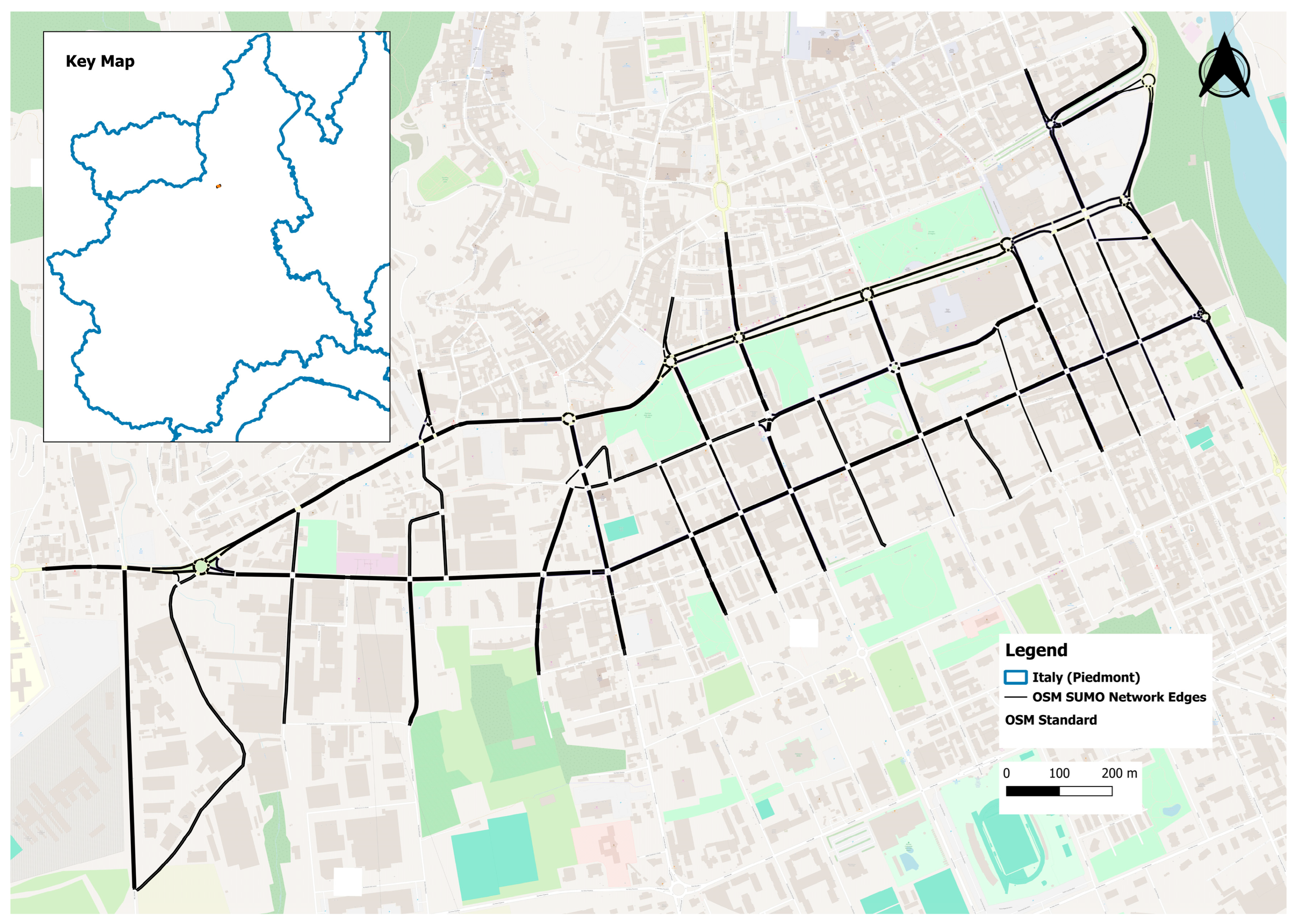
The study area selected for this analysis is located in the central part of the city of Biella, in the Piedmont region of northern Italy. The area was selected as a representative urban environment where traffic simulation models can be used to evaluate traffic management strategies. To develop a reliable microscopic traffic simulation model, it is necessary to calibrate and validate it using observed traffic data. However, before such calibration can be performed, traffic data from external sources must be integrated with the road network used in the simulation model. Therefore, the first step consists of merging the simulation network with traffic datasets, which represents the primary objective of this study.

After clipping the network to the study area boundary, the simulation network contains 194 nodes and 360 edges. The road network comprises multiple road classes, including secondary, tertiary, residential, and unclassified roads. A comparable road network was also obtained from the FCD platform, which contains 366 road segments within the same study area.

Although the number of segments is similar between the two datasets, important differences exist. In several locations, the traffic dataset provides finer road segmentation, resulting in multiple traffic segments corresponding to a single edge in the simulation network. Conversely, some residential and unclassified roads present in the simulation network are not included in the observed traffic dataset, which partly explains the discrepancy between the two networks.

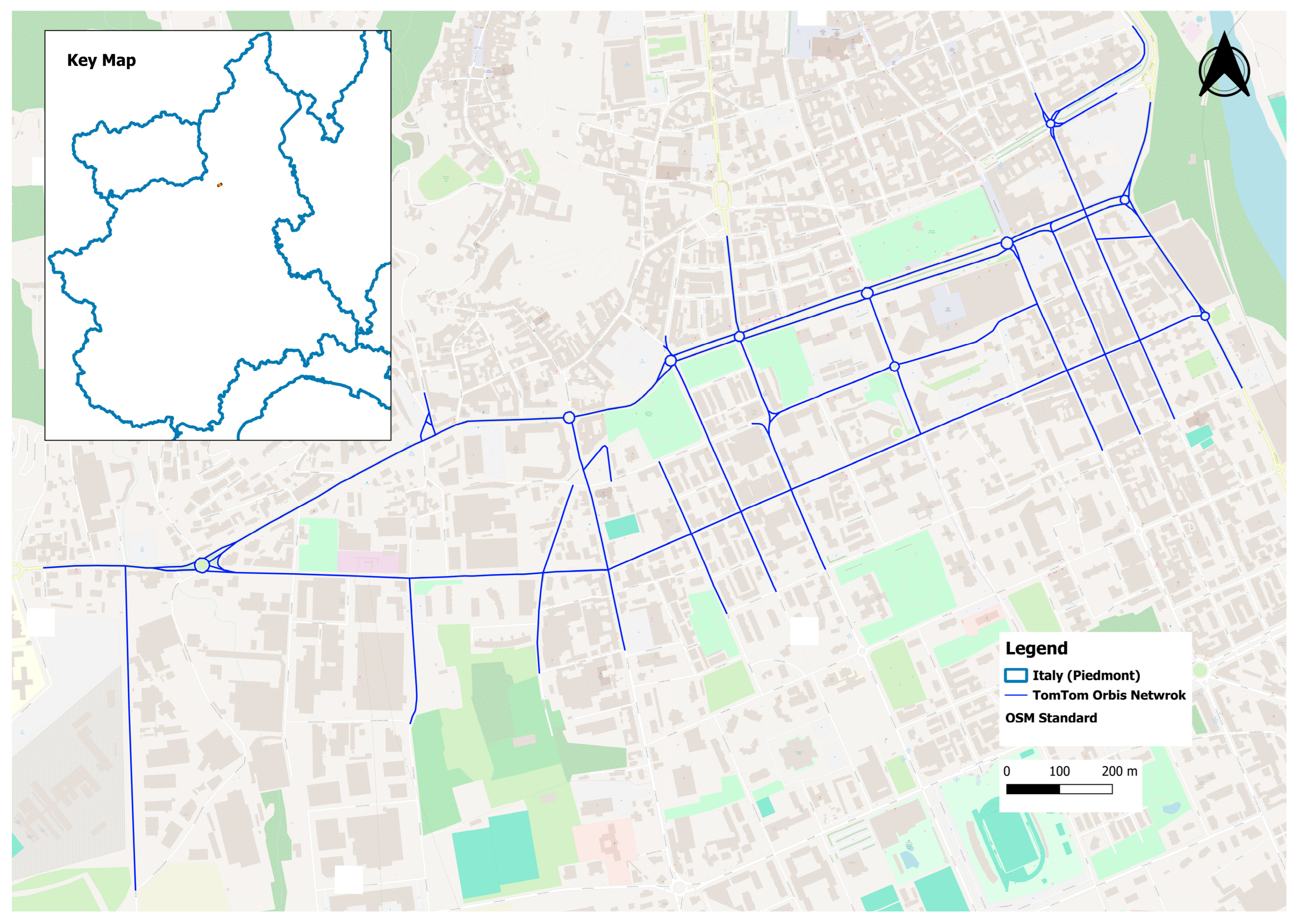
Figure 1 illustrates the simulation network edges exported as a GeoJSON dataset, which includes only the road segments and excludes junctions and connections. Figure 2 presents the corresponding FCD road network covering the same study area.

The traffic data used in this study correspond to weekday traffic conditions during the Autumn–Winter period from September 2024 to March 2025, aggregated at hourly time intervals.

2.4. Dataset Differences and Integration Objectives

Although both datasets represent the same underlying road infrastructure, several structural differences exist between the OSM-derived simulation network and the FCD traffic network, requiring a specific process to integrate traffic information between the two datasets.

First, the two networks do not share a common identifier field. Edges in the simulation network are identified by unique IDs generated during the network conversion process, whereas the FCD dataset uses proprietary segment identifiers. Consequently, a direct attribute join between the two datasets is not possible. Second, road segmentation differs between the datasets. In many cases, a single edge in the simulation network corresponds to multiple segments in the traffic dataset, while in other cases multiple simulation edges correspond to a single segment. These 1:N and N:1 relationships complicate the direct transfer of traffic attributes between the networks.

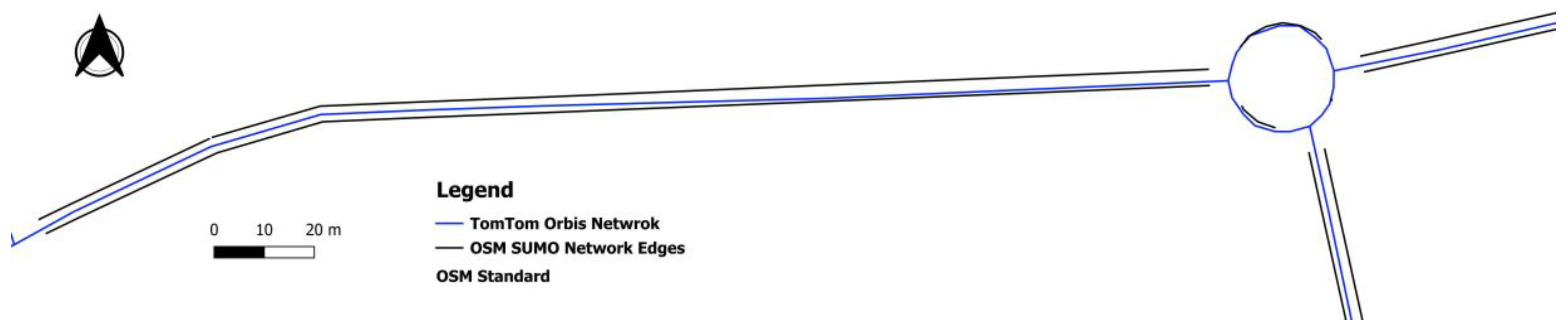
Another issue to be managed is the edge directions. In the simulation network, each direction is represented by a separate edge. In contrast, the traffic dataset often represents bidirectional roads using two vectors along the same geometric line, resulting in overlapping directional information. Furthermore, slight geometric differences exist between the two datasets, including variations in segment length, spatial alignment, and road curvature. These discrepancies arise because the networks are generated from different mapping processes and data sources.

These differences highlight the need for a spatial matching procedure capable of linking traffic segments with the corresponding edges of the simulation network. Figure 3 illustrates an example of spatial differences between the two networks in the study area, highlighting differences in segmentation and geometric representation.

3. Methodology

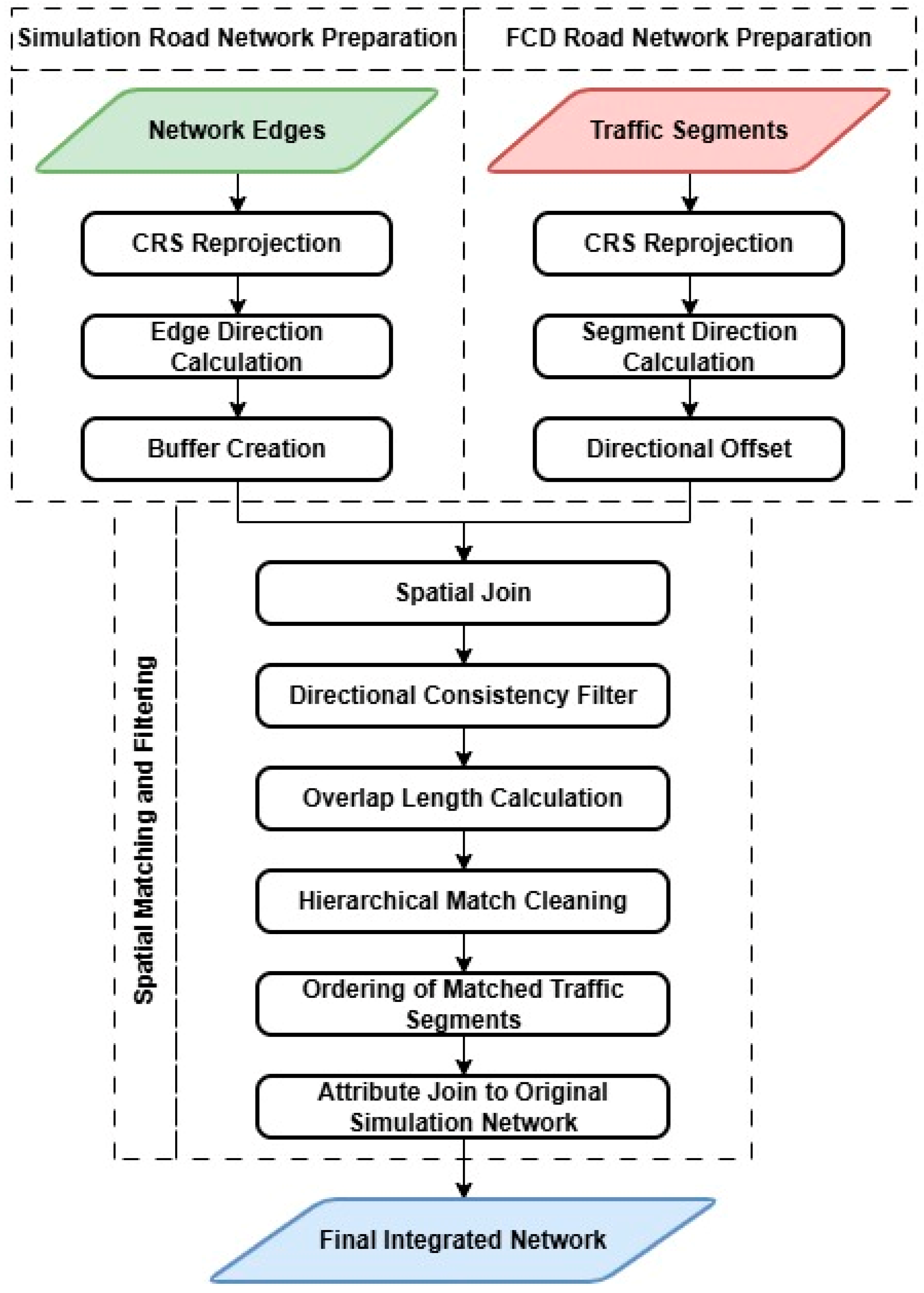
The methodology adopted to harmonize traffic data with the simulation road network is illustrated in Figure 4. The framework consists of three main stages: preparation of the simulation road network, preparation of the FCD road network, and spatial matching and filtering to associate traffic segments with the corresponding edges of the simulation network. All spatial processing steps were performed using QGIS.

3.1. Simulation Road Network Preparation

The simulation network edges, exported in GeoJSON format using the WGS84 coordinate reference system (EPSG:4326) explained in Section 2.1, are imported into QGIS for further spatial processing. For compatibility with other datasets used in the analysis, particularly the FCD road network, the layer is converted to a Shapefile, although the workflow could also be performed directly using GeoJSON layers.

The dataset is then reprojected from WGS84 (EPSG:4326) to UTM Zone 32N (EPSG:32632), which is appropriate for northern Italy and enables spatial operations to be performed using metric units. This step is necessary because subsequent geometric operations, such as buffer creation, length calculations, and spatial overlap analysis, require measurements in meters rather than degrees.

To characterize the direction of each edge, a directional attribute (azimuth) is computed based on the start and end points of the edge geometry using the QGIS Field Calculator. This operation assigns a directional value to each edge representing its orientation within the range of 0–360°, consistent with standard azimuth conventions.

Finally, a 3 m buffer is generated around each edge using flat end caps and without dissolving adjacent features. The buffer accounts for geometric discrepancies between datasets and ensures that nearby traffic segments can be captured during the subsequent spatial matching process. This value is selected based on initial visual inspection and preliminary trial analyses of geometric misalignment between the datasets. The buffer size can be adjusted depending on the degree of misalignment and should be large enough to capture as many potential matches as possible. Including segments with opposite directions does not introduce issues, as these are removed during directional filtering. However, excessively large buffers may capture adjacent parallel links with similar directions (e.g., service roads and main corridors), which can lead to incorrect matches due to high directional consistency and overlap ratios.

3.2. FCD Road Network Preparation

The FCD road network data is downloaded from the ORBIS map in Shapefile format using the WGS84 coordinate reference system (EPSG:4326). The dataset is then imported into QGIS for spatial preprocessing.

To ensure consistency with the simulation road network, the dataset is reprojected to UTM Zone 32N (EPSG:32632). Using the same projected coordinate reference system allows all subsequent spatial operations to be performed in metric units and ensures geometric compatibility between the two datasets.

A directional attribute (azimuth) is then computed for each segment based on the start and end points of the segment geometry using the QGIS Field Calculator. This results in orientation values ranging from 0° to 360°, consistent with the convention used for the simulation network.

In this dataset, bidirectional roads are represented by two overlapping line features, each corresponding to a different travel direction. To avoid spatial ambiguity, a 1.5 m right-side offset is applied using the QGIS Geometry by Expression tool. This offset separates the two directional representations geometrically while preserving their directional attributes, allowing them to be distinguished during the spatial matching stage. The value is determined based on the typical lateral displacement observed between segments and is sufficient to separate overlapping features and slightly shift them toward lane centers. When segments are already spatially separated, the offset does not significantly alter their correspondence with the simulation network.

The buffer and offset values are defined based on an initial inspection of geometric alignment between datasets and can be adjusted to balance the inclusion of candidate matches and the reduction in false associations. In practice, the buffer size plays a more critical role in capturing potential matches during the spatial join phase, while the offset primarily serves to separate overlapping directional features. An appropriate buffer value depends on the degree of geometric misalignment and should be selected to maximize candidate capture while limiting the inclusion of unrelated parallel links.

3.3. Spatial Matching and Filtering

After preparing both datasets, a spatial matching procedure is applied to associate traffic segments with the corresponding edges of the simulation network. The process includes spatial joining, directional filtering, overlap-based selection, and ordering of matched segments.

3.3.1. Spatial Join

A Join by Location operation is performed in QGIS to associate the simulation network with the traffic dataset. The 3 m buffer layer generated around the network edges is used as the input layer, while the offset traffic segments is used as the join layer. The spatial predicate Intersects is applied, and the join is configured as a one-to-many relationship.

Through this operation, attributes from the traffic dataset, particularly the segment identifier, are transferred to the buffered network layer. If an edge does not intersect any segment, no attributes are assigned. Otherwise, due to differences in network segmentation, the join may produce either one-to-one or one-to-many relationships, where a single simulation edge corresponds to one or multiple segments.

3.3.2. Directional Consistency Filtering

Because spatial proximity alone may associate simulation network edges with traffic segments representing an opposite travel direction, a directional consistency filter is applied. The angular difference between the orientation of each edge and the corresponding segment is computed to verify whether the two geometries represent a similar direction of travel.

A new attribute representing the angular difference is calculated to measure the absolute difference between the edge direction and the segment direction, while accounting for the circular nature of angular measurements (0–360°). The resulting value ranges between 0° and 180°, representing the minimum directional difference between the two geometries.

Based on this measure, valid matches are identified using a directional threshold of 45°. Matches with an angular difference of 45° or less are retained to ensure directional consistency between the paired geometries while allowing a tolerance for geometric variability. This threshold represents a balance between maintaining consistent travel direction and accounting for curvature or irregularities in road geometry. In addition, cases in which no segment is associated with an edge are preserved to maintain complete simulation network coverage for subsequent analysis.

3.3.3. Overlap Length Calculation

Despite the directional filtering step, some edges may still be associated with multiple segments. This situation typically occurs near intersections where edges are relatively short or where the spatial buffer captures the endpoints of adjacent segments. To distinguish the most relevant matches, the geometric overlap length between edges and segments is computed.

An intersection operation is performed between the offset FCD dataset and the buffer-joined layer. The resulting geometries represent the overlapping portions between the two datasets. For each intersecting feature, the overlap length is calculated and stored as an attribute.

The computed overlap length is then associated with the corresponding edge–segment pair in the joined dataset. To normalize this measure, an overlap ratio is calculated by dividing the overlap length by the total length of the corresponding traffic segment. This ratio represents the proportion of each segment that overlaps with the corresponding simulation network edge and provides a quantitative indicator for selecting the most representative match.

3.3.4. Hierarchical Match Cleaning

To resolve cases where multiple segments remain associated with a single simulation network edge, a hierarchical selection procedure is applied. This procedure combines directional consistency, overlap ratio, and edge length criteria to retain the most appropriate matches while preserving complete network coverage.

First, edges that do not intersect any segment are retained without modification. If an edge is associated with only one segment, the match is preserved directly.

For edges with multiple potential matches, the selection depends on edge length. For edges longer than or equal to 10 m, traffic segments covering at least 45% of their length within the overlap region are retained. If none of the candidates satisfy this threshold, the segment with the maximum overlap ratio is selected. A slightly relaxed threshold, compared to stricter values (e.g., 50%), is adopted to avoid excluding valid matches due to minor geometric misalignments while still ensuring that only representative segment overlaps are retained.

For short simulation network edges (<10 m), where geometric overlap may be less reliable, the segment with the smallest angular difference relative to the edge direction is selected.

This hierarchical filtering procedure produces a cleaned dataset in which each simulation edge is associated with the most appropriate segment or segments while minimizing false matches.

3.3.5. Ordering of Matched Traffic Segments

In some cases, a single edge remains associated with multiple segments after the spatial matching and filtering stages. For subsequent analyses, such as sequencing segments, aggregating speed or travel time information, or defining detector locations along the simulation network, it is necessary to establish an order among the matched segments.

To address this, a new integer ordering attribute is introduced. This attribute is assigned only to edges associated with more than one segment. The ordering is determined based on the distance between the start point of the edge and the midpoint of each corresponding segment. The segment whose midpoint is closest to the start of the edge is assigned an order value of 1, the next closest segment is assigned 2, and so on.

The midpoint of each segment is approximated using its centroid, while the reference position of the edge is defined by its start point. For each edge, the distances to all associated segment centroids are calculated and sorted in ascending order. The relative position of each distance in this ordered list defines the value of the ordering attribute.

This procedure is implemented in QGIS using aggregation functions within the Field Calculator, grouped by the simulation network edge identifier. For edges with only one matched segment, or with no associated segment, the ordering field remains NULL, as no ordering is required in these cases.

3.3.6. Attribute Join and Final Integrated Layer

The cleaned traffic dataset attributes are joined back to the original network GeoJSON layer using a Join by Attribute operation in QGIS with a one-to-many relationship. The edge identifier is used as the key field to associate the matched segment identifiers and their corresponding attributes from the buffer-based matching layer with the original network geometry.

After completing the attribute join, the resulting dataset is reprojected back to the WGS84 coordinate reference system (EPSG:4326) and exported in GeoJSON format. In the final integrated dataset, each edge is associated with the corresponding segment identifier(s) or remains NULL where no match is available.

This structure enables the subsequent integration of hourly traffic statistics, which can be linked to the network using the segment identifier as the key field.

3.4. Detector-Based Representation of Multiple Matches

In cases where a single simulation network edge is associated with multiple traffic segments, differences in segmentation between the simulation network and the traffic dataset lead to multiple traffic measurements (e.g., speed or travel time) corresponding to a single edge. To address this issue, a detector-based representation is introduced as part of the methodology. The objective is to preserve the segmentation of the traffic dataset while maintaining the simulation network’s structure.

Lane area detectors (E2 detectors) available in the SUMO platform [25] are used to represent the spatial distribution of the matched traffic segments along each simulation edge. For edges associated with multiple segments, multiple detectors are placed along the edge according to the spatial ordering defined in Section 3.3.5, with each detector corresponding to one matched segment. Detector placement is implemented through a Python script that reads the matched dataset and automatically generates the detector configuration file.

This representation enables the extraction of simulation outputs (e.g., speed, flow, and occupancy) at locations consistent with the segmentation of the traffic dataset, allowing a more accurate comparison between simulated and observed traffic parameters. By integrating detector placement into the workflow, the framework preserves one-to-many relationships between simulation edges and traffic segments without modifying the network geometry, extending the matching process to a simulation-ready representation of traffic data.

4. Results and Discussion

The methodology described in Section 3 was applied to the study area presented in Section 2.3. The results of the spatial matching process are analyzed to evaluate the integration between the simulation network and the traffic dataset.

4.1. Matching Results and Dataset Structure

The final output of the proposed methodology is a GeoJSON layer representing the simulation network edges enriched with attributes derived from the traffic dataset. The resulting attribute table establishes a relationship between the network edges and the corresponding traffic segments. Each edge is associated with the identifier of the matched segment or remains NULL if no corresponding segment is found.

The attribute table of the integrated dataset includes several fields describing characteristics of both datasets. These include the simulation edge identifier, matched traffic segment identifier, and additional geometric and directional indicators used during the matching procedure. For each pair of matched segments, the dataset stores the edge length, segment length, azimuth angles of both geometries, angular difference, overlap length, overlap ratio, and the ordering attribute assigned when multiple segments correspond to a single edge. In addition, road attributes such as the speed limit from the simulation dataset (m/s) and the traffic dataset (km/h) are preserved.

Table 1. Example rows of the integrated dataset.

Simulation Road Network Dataset				FCD Traffic Dataset
OSM id	Max Speed (m/s)	Length (m)	Angle	id	Segment id	Length (m)	Speed Limit (km/h)	Angle	Angular Difference	Overlap Length (m)	Overlap Ratio	Multiple Matches Order
-1009845454	13.89	102.08	158.056	338	1166751986752520193	110.912	50	157.896	0.16	102.134	0.921
-1078137846	27.78	39.04	274.434	317	1166751986720309249	11.712	30	270.687	3.747	8.165	0.697	1
-1078137846	27.78	39.04	274.434	315	1166751986720276481	39.182	30	275.569	1.135	31.118	0.794	2
-1078137847	13.89	47.19	155.012	364	1166751986776145921	58.261	50	154.425	0.587	47.232	0.811
-163744716#0	13.89	135.69	68.188	354	1166751986775752705	18.148	50	65.291	2.897	10.44	0.575	1
-163744716#0	13.89	135.69	68.188	352	1166751986775719937	72.249	50	69.009	0.821	72.249	1	2
-163744716#0	13.89	135.69	68.188	350	1166751986775687169	22.161	50	67.021	1.167	22.161	1	3
-163744716#0	13.89	135.69	68.188	348	1166751986775654401	36.639	50	67.389	0.799	30.706	0.838	4
-199961727#0	13.89	687.96	187.04
-199961727#1	13.89	30.62	241.465

presents an example of several rows from the final dataset, illustrating the relationship between the edge identifiers and the matched segment identifiers, as well as selected geometric and directional attributes produced during the matching process.

Once the matching is completed, the id field of the traffic dataset allows the integration of traffic statistics with the simulation network. Using this identifier as a key field, hourly traffic information can be directly joined to the simulation network. As an example, the hourly dataset corresponding to the Autumn–Winter weekday period from September 2024 to March 2025 between 08:00 and 09:00, representing the morning peak hour, was joined to the integrated network. This operation enriches the simulation network with observed traffic indicators such as average travel time, median travel time, average speed, harmonic average speed, median speed, standard deviation of speed, and measurement counts.

The matching statistics for the study area indicate that the majority of edges are successfully associated with traffic segments. Out of 360 edges in the simulation network, 257 exhibit a one-to-one relationship with a single segment, while 40 edges are associated with multiple segments. Among these, 25 edges correspond to two segments, 7 to three segments, and 8 to four segments. In addition, 63 edges have no corresponding segment, indicating the absence of traffic data (

Table 2. Distribution of the number of matched traffic segments associated with each simulation network edge in the study area.

Number of Matched Segments per Edge	Count	Percentage (%)
0	63	17.5
1	257	71.4
2	25	6.95
3	7	1.95
4	8	2.2

). Overall, more than 80% of the network edges are successfully linked with traffic information, demonstrating the effectiveness of the proposed methodology.

As a first assessment, the integrated dataset was visually inspected in QGIS. For most matched cases, the segments align well with the corresponding edges, confirming the effectiveness of the spatial, directional, and overlap-based filtering steps. However, some limitations were identified. Unmatched edges are often associated with residential or unclassified roads that are not included in the traffic dataset, resulting in missing traffic information.

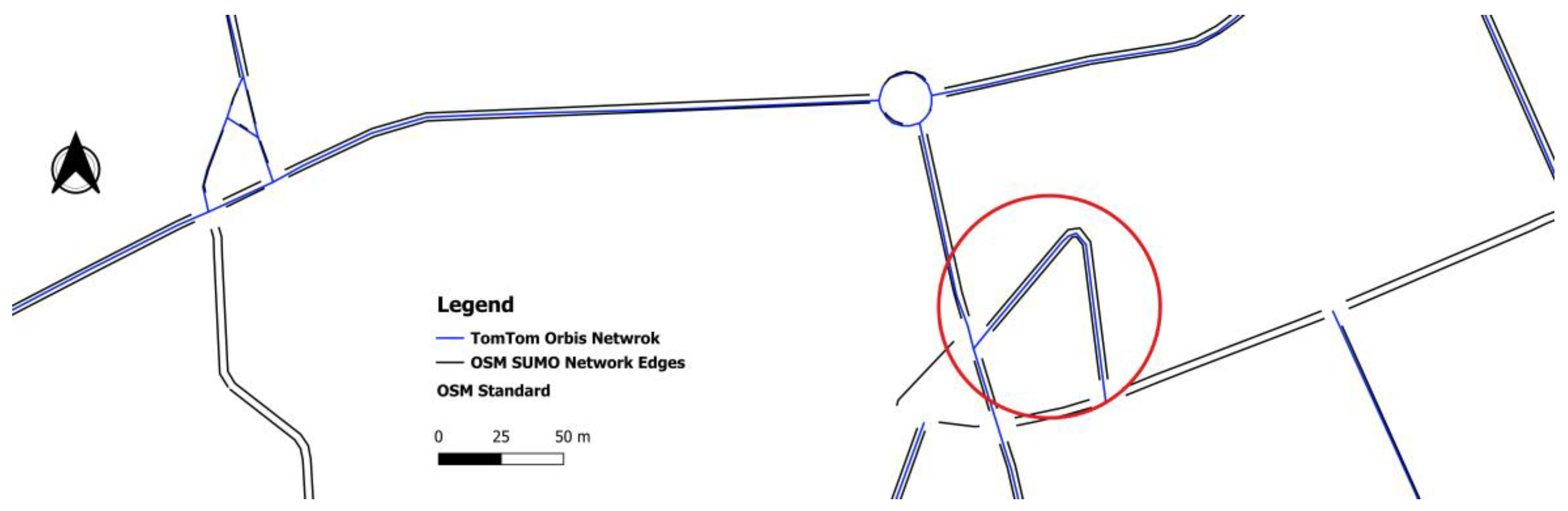
Additional discrepancies occur in locations where geometric representations differ, particularly along curved roads or polylines with multiple vertices. In such cases, the computed angular difference may exceed the filtering threshold, preventing valid matches. An example of this situation is illustrated in Figure 5, where geometric curvature leads to directional inconsistency.

Further mismatches may occur near intersections or roundabouts, where the overlap-based filtering step may remove potential matches due to the relatively small overlap ratio between segments. Nevertheless, these cases typically occur on short or low-priority road segments and therefore have limited impact on the overall integration of the simulation network with traffic data.

Validation of Matching Results

To quantitatively assess the performance of the proposed methodology, a manual validation was conducted on all 360 simulation network edges. Each edge was evaluated by comparing the matched traffic segments with the true corresponding segments identified through visual inspection in QGIS. Validation was performed using the simulation network edges as the reference unit, as this represents the fixed structure required for simulation, while traffic data must be consistently integrated onto it.

For each edge, the numbers of true matches, detected matches, and correctly matched segments were recorded. Based on these values, performance metrics were computed, including precision and recall. Precision is defined as the ratio of correctly matched segments to the total number of detected matches, while recall represents the ratio of correctly matched segments to the total number of true segments.

The validation results indicate an overall precision of 97.8% and a recall of 96.2%, demonstrating that the proposed methodology achieves high accuracy in identifying relevant matches while maintaining a limited number of false and missing associations. In terms of edge-level accuracy, 346 out of 360 edges (96.1%) were correctly matched, while 3 edges (0.8%) were partially correct and 11 edges (3.1%) were incorrectly matched. These results confirm the robustness of the proposed approach.

A more detailed analysis shows that, out of 360 edges, 63 resulted in no match. Among these, 60 correspond to cases where no FCD data are available, while 2 are associated with directional filtering errors (Figure 5), in which valid segments were excluded due to angular differences greater than 45°. One additional case corresponds to a missing match in a roundabout due to offset-related geometric misalignment. Among the 257 one-to-one matches, 249 were correctly identified. The remaining cases include 2 false matches, where segments were incorrectly assigned despite low overlap but acceptable angular difference, and 6 missing matches, mainly occurring in roundabouts due to horizontal misalignment, lack of finer FCD segmentation, or offset-related discrepancies. For the 40 one-to-many matches, 37 were correctly identified. The remaining cases include 1 missing match, where one of the true segments was not captured due to geometric misalignment, and 2 cases affected by the overlap threshold, where valid segments were excluded because their overlap ratio was below the adopted threshold. Overall, 14 false matches were identified, including a small number of partially correct cases, while 8 edges showed inconsistencies between the number of detected and true matches.

The analysis of mismatches indicates that most errors are associated with missing matches rather than incorrect associations. These cases are primarily caused by geometric discrepancies between datasets, including horizontal misalignment, and, in a few cases, insufficient overlap or directional filtering effects. In particular, mismatches were observed near roundabouts and intersections, where differences in network representation and segmentation are more pronounced. Despite these localized issues, the high precision and recall values indicate that by the adopted thresholds and filtering criteria provide an acceptable matching performance for the integration of traffic data with the simulation network.

4.2. Application of Detector-Based Representation in Simulation

The detector-based representation introduced in Section 3.4 is applied to the integrated dataset to illustrate its use in handling multiple matches within the simulation environment. For simulation edges associated with multiple traffic segments, multiple detectors are placed along the same edge according to the spatial ordering defined during the matching process. This enables each segment to be represented individually within the simulation while preserving the original network structure.

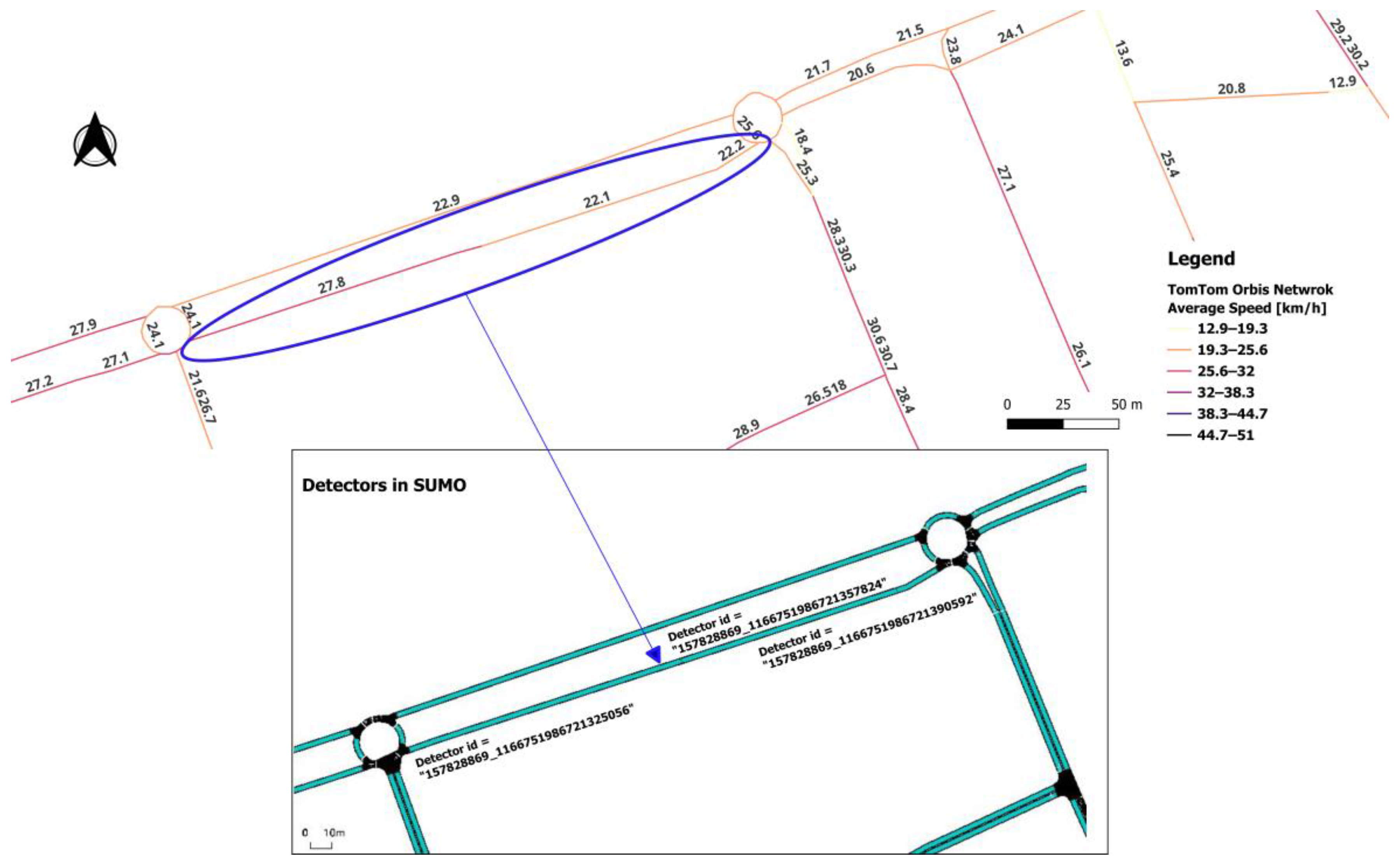
This correspondence is illustrated in Figure 6, where multiple traffic segments mapped to a single edge are represented by multiple detectors, enabling segment-level comparison of traffic variables.

The same approach can also be extended to the entire network, enabling systematic monitoring of simulation outputs and facilitating direct comparison with observed traffic data. Additionally, detector-based measurements can be used as input for model calibration or traffic demand estimation, further enhancing the integration between simulation and observations.

4.3. Transferability Analysis in an Additional Case Study

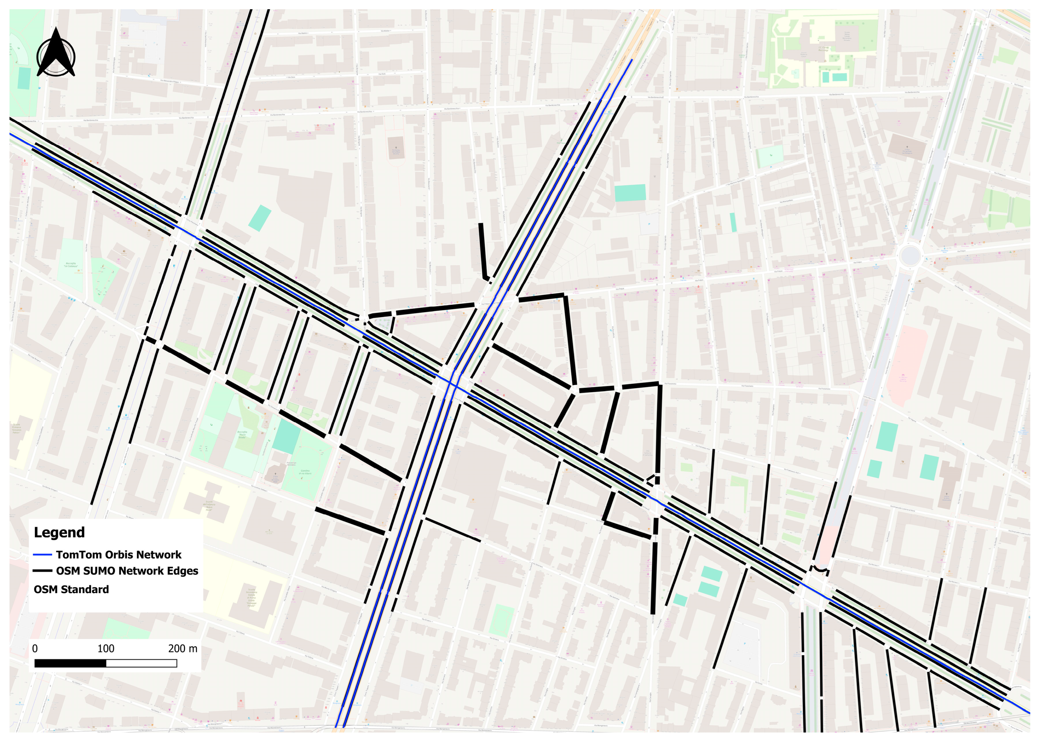
To further assess the transferability of the proposed methodology, an additional application was conducted in a different urban area located in the southwest of Turin, Italy, with a specific focus on the intersection of Corso Trapani and Corso Peschiera, including adjacent roads such as Via Frejus and Corso Racconigi (Figure 7). The traffic dataset was derived from the TomTom Traffic Stats platform [15], covering mainly primary roads and excluding minor and service roads, with the same structure described in Section 2.2. The objective of this additional application was to evaluate the applicability of the methodology across various locations.

As discussed in Section 3.1 and Section 3.2, buffer and offset values can be adjusted depending on the geometric differences between datasets. Based on an initial visual inspection, the average lateral offset between networks was estimated, confirming that an offset value of 1.5 m is suitable for the traffic dataset in most cases. To increase the capture of candidate matches before the filtering stage, a buffer value of 6 m was applied to the simulation network edges.

The results show that, following the proposed methodology, the dataset was successfully integrated with the simulation network where traffic data were available, which in this case were limited to the main roads. As a result, out of 183 simulation edges from OSM, 135 simulation edges were not matched, while 48 edges were successfully associated with traffic segments. Among these, 28 correspond to one-to-one matches and 20 to one-to-many relationships, including cases with higher segmentation (up to six segments associated with a single simulation edge). These differences are primarily due to variations in data availability (as shown in Figure 7) and segmentation schemes between the traffic dataset and the simulation network. Despite these differences, the methodology consistently identified appropriate spatial correspondences between simulation network edges and traffic segments.

Although this second case study is also based on an urban area, it presents a more complex network structure with dense intersections. The results demonstrate that the proposed framework can be applied across different locations. The methodology shows practical transferability, requiring only an initial approximation of buffer and offset parameters based on dataset characteristics, while maintaining robust matching performance.

4.4. Potential Applications

The integration of traffic information with the simulation network enables several practical applications for traffic modeling and simulation studies.

A first application is the correction and refinement of speed limits in the simulation network. Open-source data may contain inaccurate speed limit values that can affect simulation realism. For example, as shown in Table 1, an edge corresponding to OSM ID -1078137846 has a maximum speed of 27.78 m/s (100 km/h), which is unrealistic for a road located in the city center of Biella. However, the matched data indicate a speed limit of 30 km/h, derived from two associated segments. Updating these attributes with the integrated dataset can improve the network’s accuracy before simulations.

Another application is the placement of traffic detectors in microscopic simulations. While Section 4.2 focuses on their role in representing multiple matched segments along a single edge, detectors can also be used more generally to monitor traffic conditions along network links [25]. These detectors function similarly to traffic monitoring devices, such as vehicle-tracking cameras, and measure indicators such as vehicle counts, speeds, queues, and congestion conditions. By using the matched segment information, detectors can be systematically placed along the simulation network’s edges corresponding to traffic-monitoring locations. This enables the extraction of simulation outputs that are directly comparable with observed traffic data.

Such integration also enables improved simulation validation procedures. In previous work, simulation validation was performed by manually selecting representative routes and comparing simulated average speeds with observed floating car data along those routes [6]. Although this approach provided useful insights into the overall simulation performance, the validation process remained limited to aggregated route-level comparisons and required manual selection of validation paths. However, with the integrated dataset produced by the proposed framework, validation can be performed systematically at the edge level, enabling comparison of simulated and observed traffic indicators such as speed and travel time for each matched segment and time interval. This increases the spatial resolution and robustness of the validation process.

Another potential application is the estimation and calibration of traffic demand. FCD datasets provide information on vehicle movements, speeds, and traffic density at a higher spatial resolution than traditional detector networks. As discussed by Veihelmann et al. [12], high-resolution probe counts can be integrated into microscopic traffic simulations by matching commercial traffic datasets with simulation networks and using the resulting traffic counts as constraints for demand generation and route sampling. In particular, segment-level traffic counts can support route sampling, O–D matrix calibration, and demand generation procedures, enabling the development of more realistic large-scale microscopic simulations.

Overall, the integration framework presented in this study provides a flexible basis for network calibration, detector placement, simulation validation, and traffic demand generation, facilitating the use of traffic data in simulation-based transport studies.

5. Conclusions

This study presented a GIS-based framework for integrating FCD traffic data with road networks used in traffic simulation models. The proposed methodology addresses a common challenge in transportation modeling: integrating heterogeneous datasets that represent the same road infrastructure using different segmentation schemes and without shared identifiers. By combining spatial analysis techniques within a GIS environment, the framework enables the association of traffic segments with a simulation network derived from open-source data.

The methodology consists of several sequential steps, including preprocessing of the simulation network and traffic data, spatial buffering, spatial joining, directional consistency filtering, overlap-based matching, and hierarchical cleaning of candidate matches. These procedures enable the identification of spatial relationships between the two datasets while minimizing false matches due to geometric differences or segmentation inconsistencies. The workflow is implemented using standard tools in QGIS, ensuring transparency, reproducibility, and applicability without requiring complex optimization or machine learning approaches.

The proposed framework was applied to a case study in the central area of Biella, Italy. Despite structural differences between the datasets, the matching process successfully associated more than 80% of the simulation network edges with corresponding FCD traffic segments. Most matches resulted in one-to-one relationships, while a smaller proportion reflected one-to-many associations due to finer segmentation in the traffic dataset. A quantitative validation conducted on all simulation network edges showed high matching accuracy, with overall precision and recall values of 97.8% and 96.2%, respectively. The analysis also showed that most mismatches were related to missing matches caused by geometric discrepancies near roundabouts, intersections, or curved road segments, rather than incorrect associations between unrelated segments.

An additional case study conducted in a neighborhood in Turin further demonstrated the transferability of the proposed methodology across different study areas. Despite the more complex urban network structure, the methodology maintained robust matching performance, confirming that the directional and overlap-based filtering criteria are effective, while buffer and offset parameters can be adjusted according to dataset characteristics and geometric alignment conditions.

The resulting integrated dataset provides a structured link between edges modeled for simulation and traffic statistics. This enables the direct integration of hourly traffic indicators such as travel time, speed, traffic flow, and traffic variability into the simulation network. Such information can improve the reliability of traffic simulation models and support several practical applications. These include correcting network attributes such as speed limits, systematically placing traffic detectors within simulation environments, and validating simulation outputs against observed traffic data. Additionally, the framework facilitates the use of traffic observations as constraints for estimating and calibrating traffic demand in microscopic simulations.

Although the methodology demonstrated promising results, some limitations remain. Differences in network geometry, particularly near curved road segments or complex intersections, may lead to missing matches when directional thresholds or overlap criteria are applied. Furthermore, some roads in the simulation network may not be included in the traffic dataset, leading to unavoidable gaps in the integrated network. The adopted thresholds demonstrated robust performance in the presented applications; however, future research could further investigate adaptive or automated threshold selection procedures, additional geometric similarity indicators, or hybrid approaches combining GIS-based matching with machine learning techniques.

Overall, the study demonstrates that heterogeneous traffic datasets can be effectively integrated with simulation networks through a GIS-based workflow. The proposed framework offers a transferable approach for preparing enriched traffic simulation models by taking advantage of big-data traffic platforms. This can support transportation planning processes oriented toward sustainable mobility actions, which in some cases may generate side effects that should be predicted in advance to better manage the application of traffic control strategies and mobility management measures.