Robust Data-Driven Transmission-Line Parameter Estimation for Reliable and Sustainable Smart Grid Operation

Abstract

Accurate transmission-line parameters are essential for reliable, efficient, and sustainable smart grid operation, especially under increasing renewable-energy integration and data-driven grid management. However, line aging, temperature variations, and measurement outliers may cause significant deviations between actual and nominal grid models, thereby degrading the state estimation, power-flow analysis, and operational security assessment. To address these challenges, this paper proposes a robust transmission-line parameter estimation method based on a variable-projection framework. The proposed framework decomposes the original high-dimensional, strongly coupled, and non-convex joint estimation problem into two subproblems associated with line-parameter identification and operating-state calibration. An iteratively reweighted least-squares algorithm based on the Huber M-estimator is introduced to dynamically adjust measurement weights and suppress the influence of outliers. The preconditioned conjugate-gradient method is further employed to avoid the explicit inversion of large-scale normal matrices. Simulations on the IEEE 118-bus system demonstrate that the proposed method achieves a higher parameter-estimation accuracy and stronger robustness than conventional weighted least-squares and joint state-parameter estimation methods. In the base case, the proposed method reduces the RMSRE of line reactance to 0.0794%, compared with 0.1558% for WLS and 0.1126% for JSE. Under the representative 5% gross-error case, the proposed method maintains lower RMSREs of 0.9772%, 0.0875%, and 5.8536% for $R_l$, $X_l$, and $B_{sh}$, respectively. Further sensitivity tests under contamination ratios from 1% to 20%, outlier magnitude factors from 1.5 to 5.0, and different outlier-location patterns confirm that the proposed method maintains a more stable estimation accuracy than WLS, conventional JSE, and Huber-JSE without VPM under diverse bad-data conditions. In downstream operational evaluations, it reduces the branch active-power flow RMSE from 1.6842 MW to 0.7215 MW, voltage-magnitude RMSE from 0.00482 p.u. to 0.00216 p.u., and active-power-loss error from 2.4368% to 0.9327% compared with WLS. These quantitative results indicate that the proposed approach can improve the grid model accuracy under imperfect measurements, thereby supporting reliable and sustainable smart-grid operation.

1. Introduction

1.1. Motivation

The transition toward low-carbon and sustainable energy systems is accelerating the development of smart grids with a higher renewable-energy penetration, stronger operating uncertainty, and increasing dependence on measurement-driven decision-making [1,2,3]. In such systems, accurate network parameters are fundamental to state estimation, power-flow analysis, loss evaluation, voltage-security assessment, and optimal operation [4]. Transmission-line parameters, as key physical characteristics of the grid model, directly affect the reliability and efficiency of these model-based applications. Therefore, maintaining accurate and up-to-date line parameters is an important prerequisite for reliable and sustainable smart grid operation. However, these parameters are not constant in practice. Line aging and temperature fluctuations can cause parameters to gradually deviate from their nominal values [5]. In this context, the online identification of line parameters using abundant grid measurement data has become a crucial technique for improving the accuracy of power grid models.

Although measurement devices like SCADA systems, advanced metering infrastructure (AMI), and phasor measurement units (PMUs) collect large volumes of data, this data is affected by random noise, systematic biases, and abnormal outliers [6]. More importantly, line parameters and network states are tightly coupled within the physical model, resulting in a high-dimensional, nonlinear, and non-convex joint estimation problem. Traditional weighted least squares (WLS) methods are highly sensitive to bad data. The “leverage effect” caused by outliers may significantly bias estimation results, leading to poor parameter identification performance. To address these shortcomings, it is necessary to develop a modified estimation method with a high robustness to bad data.

From the perspective of sustainability-oriented grid operation, inaccurate line parameters may lead to biased power-flow results, incorrect loss evaluation, the conservative or unsafe utilization of transmission assets, and unreliable security assessment. These problems are particularly critical for renewable-rich power systems, where operating conditions fluctuate frequently and accurate grid models are required to support flexible dispatch and efficient energy delivery. Therefore, robust parameter estimation under imperfect measurement conditions is not only a modeling problem but also a key enabling technology for sustainable, resilient, and data-driven smart grids.

More specifically, the sustainability benefit of accurate line-parameter estimation is reflected in several operational aspects. First, more accurate resistance and reactance parameters reduce the mismatch between calculated and actual branch power flows, which helps operators avoid unnecessary security margins caused by model uncertainty. Second, improved resistance estimation contributes to more reliable active-power-loss evaluation, which is important for loss-aware dispatch and energy-efficiency assessment. Third, more accurate voltage and reactive-power calculations improve the assessment of voltage-security margins, especially under renewable-rich operating conditions with frequent power fluctuations. Therefore, although parameter estimation does not directly perform dispatch or control, it provides a more reliable network model that supports lower-loss, less conservative, and more renewable-accommodating smart-grid operation.

1.2. Related Work

The existing studies on transmission-line parameter estimation can be broadly classified into several thematic groups according to their mathematical formulation, measurement requirements, treatment of measurement errors, and application scenarios.

First, several studies have focused on parameter identifiability and measurement requirements. These works investigate whether transmission-line parameters can be uniquely estimated under different measurement configurations, especially when the voltage phase-angle information is unavailable or incomplete. When phase-angle information is unavailable, direct admittance-based regression may lead to inconsistent or biased estimates, whereas impedance-based intermediate modeling can improve identifiability [7]. In addition, voltage and current magnitudes measured at both ends of a line can be used to infer series impedance and shunt admittance without relying on synchronized phase-angle measurements [8]. These studies provide important theoretical foundations for line-parameter estimation. However, they mainly focus on identifiability and measurement sufficiency rather than robust estimation under corrupted measurement data.

Second, PMU/SCADA-based methods constitute an important category of practical transmission-line parameter estimation approaches. Synchronized PMU measurements can provide voltage and current phasors with a high time accuracy, which may transform the parameter estimation problem into a linear or nearly linear formulation under ideal measurement conditions [9,10]. When full PMU deployment is unavailable, SCADA/PMU hybrid methods and multi-period measurements can improve redundancy and estimation stability [11,12]. These methods are attractive from an engineering perspective because they can use existing monitoring infrastructure. However, their performance is often affected by measurement noise, data synchronization quality, phase-angle availability, and bad data. In particular, direct regression or conventional WLS formulations may suffer from biased estimates when gross errors or non-Gaussian disturbances are present.

Third, several studies have investigated measurement-error calibration and phase-angle error correction. Practical PMU measurements may contain magnitude errors, phase-angle delays, and inconsistent angle references at both terminals of a transmission line. To address these problems, online PMU error correction and phase-angle difference calibration methods have been developed [13,14,15]. These methods can reduce error amplification caused by inaccurate phasor references and improve the reliability of PMU-based parameter calculation. Non-iterative synchrophasor-based parameter estimation methods have also been proposed to improve computational efficiency [16]. Nevertheless, these studies usually focus on specific measurement error sources or measurement configurations, while general outlier suppression and robust multi-period state-parameter calibration remain insufficiently explored.

Fourth, robust, non-Gaussian, recursive, and joint estimation methods have been developed to address imperfect measurement conditions. Under non-Gaussian noise conditions, hybrid distribution and maximum-likelihood methods can provide a better robustness than conventional LS/TLS formulations [17]. EKF-based methods can recursively estimate phasors and slowly varying line parameters using online measurements [18]. In addition, joint state-parameter estimation methods estimate system states and line parameters simultaneously by exploiting their physical coupling [19,20]. However, EKF-based methods depend on recursive linearization and assumed parameter evolution models, while conventional JSE usually leads to a high-dimensional nonlinear optimization problem. Moreover, robust M-estimators are often applied directly to the original coupled residual minimization problem, without explicitly exploiting the separable structure between time-invariant line parameters and time-varying operating states.

Fifth, recent studies have further emphasized the role of PMU-enabled synchronized measurements and smart-grid technologies in sustainable power system operation. PMU-driven line-parameter estimation with variable noise models and Kalman-filter-based estimation using synchronized phasor measurements have been investigated to improve practical measurement modeling [21,22]. Meanwhile, PMU installation planning and PMU-supported monitoring have been widely discussed in the context of smart grids [23,24]. More broadly, smart energy systems and renewable-rich grids require accurate and adaptive network models to support real-time monitoring, renewable integration, and efficient operation [25]. These studies highlight the importance of accurate measurement-driven model calibration for sustainable smart grids, but they do not fully address the combined requirements of robustness, computational efficiency, and multi-period state-parameter coupling.

Finally, transmission-line parameter estimation has also been extended to specialized scenarios, including non-transposed three-phase lines, three-phase network-wide parameter error identification, frequency-dependent wideband estimation, and series-compensated transmission lines [26,27,28,29]. These studies broaden the application scope of line-parameter estimation under unbalanced, frequency-dependent, or compensated operating conditions. However, they are usually designed for specific physical scenarios and do not directly focus on robust multi-period calibration of standard transmission-line parameters under corrupted PMU/SCADA-type measurements.

To provide a clearer critical comparison,

Table 1. Critical comparison of representative transmission-line parameter estimation methods.

Method Category	Representative References	Typical Data Type	Robustness to Noise/Bad Data	Computational Cost	Treatment of Outliers	Main Limitation
Identifiability-oriented methods	[7,8]	Voltage/current magnitudes, partial phasor data	Usually not the main focus	Low to moderate	Not explicitly considered	Focus mainly on theoretical identifiability rather than corrupted data
PMU/SCADA direct and hybrid estimation	[9,10,11,12]	Synchronized PMU phasors, SCADA measurements, multi-period data	Moderate under high-quality measurements	Low to moderate	Usually handled by WLS weighting or preprocessing	Sensitive to measurement quality, synchronization errors, and bad data
Measurement-error and phase-angle calibration	[13,14,15,16]	Dual-end PMU phasors, angle-difference measurements	Good for specific systematic errors	Moderate	Mainly corrects phasor magnitude or angle errors	Focuses on specific error sources rather than general gross outliers
Non-Gaussian robust estimation	[17]	PMU/SCADA measurements with non-Gaussian noise	Relatively high	Moderate to high	Uses non-Gaussian or maximum-likelihood modeling	Robustness is improved, but state-parameter separability is not fully exploited
EKF-based estimation	[18]	Time-series phasor or SCADA/PMU data	Moderate under properly modeled noise	Moderate to high	Usually handled through covariance tuning	Requires recursive linearization and assumed parameter evolution models
Conventional JSE methods	[19,20]	Multi-period measurements with coupled states and parameters	Better physical consistency than separate estimation	High	Usually limited unless combined with robust loss	Leads to high-dimensional nonlinear coupled optimization
PMU-enabled smart-grid and sustainability-oriented studies	[21,22,23,24,25]	PMU/smart-grid monitoring data	Scenario-dependent	Moderate	Usually not the main focus	Emphasizes monitoring or sustainable operation more than robust parameter calibration
Three-phase, wideband, and specialized methods	[26,27,28,29]	Three-phase PMU data, wideband synchrophasors, compensated-line data	Scenario-dependent	Moderate to high	Depends on the specific formulation	Designed for specialized physical scenarios
Proposed robust VPM method	This paper	Multi-period PMU/SCADA-type measurements	High under Gaussian noise and gross errors	Moderate; reduced by block structure and PCG	Huber IRLS weights embedded into variable projection	Field-data validation and extension to broader dynamic scenarios remain future work

summarizes the main characteristics and limitations of representative transmission-line parameter estimation methods.

As shown in Table 1, the existing methods have made important contributions from different perspectives, including identifiability analysis, PMU/SCADA data utilization, phase-error correction, non-Gaussian noise modeling, recursive tracking, and specialized three-phase or wideband applications. However, robustness, computational tractability, and multi-period state-parameter coupling are usually addressed separately. Conventional WLS is computationally efficient but lacks robustness to gross errors. EKF and JSE can model state-parameter coupling, but they either require dynamic evolution assumptions or suffer from high-dimensional coupled optimization. Robust M-estimation improves resistance to bad data, but it is often directly applied to the original estimation problem without exploiting the separable structure between time-invariant line parameters and time-varying operating states. Motivated by these gaps, this paper develops a robust variable-projection framework that combines multi-period information aggregation, Huber IRLS-based outlier suppression, and block-structured state calibration for transmission-line parameter estimation under imperfect PMU/SCADA-type measurements.

Compared with existing robust and joint estimation methods, the mathematical distinction of this work lies in the way the coupled state-parameter estimation problem is reformulated and solved. Conventional WLS solves the original measurement-fitting problem with fixed Gaussian weights and therefore remains sensitive to gross errors. Conventional JSE usually estimates system states and line parameters in a fully coupled manner, which leads to a high-dimensional nonlinear optimization problem. EKF-based approaches rely on recursive linearization and a predefined dynamic evolution model for slowly varying parameters, whereas the present work treats line parameters as time-invariant physical quantities shared by multiple operating snapshots and calibrates the corresponding time-varying operating states simultaneously. Although M-estimators have been used for robust estimation, they are commonly applied directly to the original coupled residual minimization problem. In contrast, this paper embeds the Huber M-estimator into a variable-projection framework, where the time-varying state variables are locally eliminated or calibrated, and the line parameters are updated through a reduced multi-period parameter-estimation subproblem. Therefore, the novelty of the proposed method is not the independent use of Huber weighting or variable projection, but their integration into a robust projected joint state-parameter estimation formulation specifically designed for transmission-line parameter calibration under imperfect PMU/SCADA-type measurements. To highlight the mathematical distinctions of the proposed method,

Table 2. Mathematical differences between the proposed method and related estimation methods.

Method	Basic Formulation	Main Limitation	Difference of the Proposed Method
WLS	Fixed-weight least-squares estimation under Gaussian noise	Sensitive to gross errors and leverage effects	Uses Huber IRLS weights to adaptively reduce outlier influence
Conventional JSE	Simultaneous estimation of states and parameters in one coupled problem	High-dimensional nonlinear optimization; strong state-parameter coupling	Uses variable projection to eliminate/calibrate state variables and solve a reduced parameter problem
EKF-based estimation	Recursive state/parameter tracking with dynamic model assumptions	Requires linearization and parameter evolution model; mainly suitable for online tracking	Uses multi-period batch estimation with time-invariant line parameters shared across snapshots
M-estimation	Robust residual penalty applied to estimation objective	Often applied directly to the original coupled problem	Embeds Huber M-estimation into the projected state-parameter framework
PMU/SCADA-based direct methods	Parameter calculation or regression using synchronized or hybrid measurements	Often sensitive to measurement availability, angle errors, or bad data	Uses a measurement-selection model, multi-period information aggregation, robust weighting, and latent state calibration

provides a comparative analysis of the basic formulation, main limitations, and the specific differences of this work against conventional methods.

1.3. Contributions

To address the aforementioned challenges, this paper proposes a robust data-driven transmission-line parameter estimation framework for reliable and sustainable smart grid operation. The main contributions are summarized as follows:

(1) A sustainability-oriented grid model calibration framework is proposed to improve the accuracy of transmission-line parameters under imperfect measurement conditions. By enhancing the reliability of network models, the proposed method supports the state estimation, power-flow analysis, and security assessment in sustainable smart grids.

(2) A robust variable-projection formulation is developed for the multi-period joint state-parameter estimation problem. Different from conventional JSE, which solves the coupled state and parameter variables simultaneously, the proposed formulation exploits the separable structure between time-invariant line parameters and time-varying operating states. By using block-diagonal state Jacobians and vertically concatenated parameter Jacobians across multiple time periods, the original high-dimensional normal equation is transformed into a reduced parameter-estimation problem with locally calibrated state variables.

(3) A Huber M-estimator-based IRLS mechanism is embedded into the variable-projection process. In contrast to conventional WLS with fixed measurement weights, the proposed method updates robust weights according to standardized residuals and incorporates them into both the parameter-identification and state-calibration subproblems. This design reduces the leverage effect of abnormal measurements while preserving the multi-period information aggregation capability of the joint estimation framework.

(4) A preconditioned conjugate-gradient solver is employed to avoid the explicit inversion of large-scale normal matrices, making the proposed framework more suitable for multi-period measurement datasets.

The remainder of this paper is organized as follows. Section 2 formulates the transmission-line parameter estimation problem and discusses its role in measurement-driven smart grid modeling. Section 3 presents the proposed robust variable-projection estimation framework. Section 4 evaluates the proposed method on the IEEE 118-bus system and further analyzes its robustness and potential benefits for sustainable smart grid operation. Section 5 concludes the paper.

2. Materials and Methods

2.1. $\pi$-Equivalent Circuit of Transmission Lines

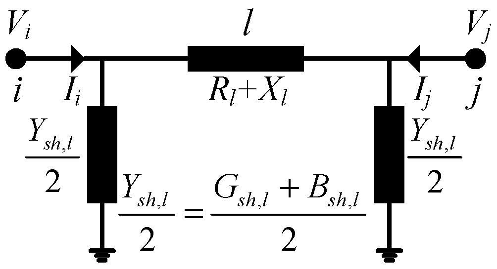
In steady-state power system analysis, transmission lines are usually modeled using the positive-sequence $\pi$-equivalent circuit. As shown in Figure 1, this model represents a line $l=(i,j)$ with a series impedance $Z_l=R_l{+jX}_l$ combined with two shunt admittances to ground, each equal to $Y_{sh,l}/2=G_{sh,l}{/2+jB}_{sh,l}/2$. $R_l$ and $X_l$ denote the series resistance and reactance of the line, and $G_{sh,l}$ and $B_{sh,l}$ represent the shunt conductance and susceptance to ground, respectively.

The line parameters to be estimated are defined as $p_l=\left(R_l,X_l,G_{sh,l},B_{sh,l}\right)$ and $p=\left(p_1^T,p_2^T,\dots ,p_L^T\right)$ denotes the full network line-parameter vector. Generally, the series impedance is usually converted into series admittance. The specific relationship between impedance and admittance is

$$y_l=g_l+j{b}_l={\displaystyle \frac{1}{R_l+j{X}_l}}={\displaystyle \frac{R_l-j{X}_l}{R_l^2+X_l^2}}$$

(1)

Therefore, the $g_l$ and $b_l$ are

$$g_l={\displaystyle \frac{R_l}{R_l^2+X_l^2}},b_l=-{\displaystyle \frac{X_l}{R_l^2+X_l^2}}$$

(2)

Define the system state vector $s^{\left(t\right)}$ as the set of RMS voltage phasor magnitudes $\left|V_i^{\left(t\right)}\right|$ in per unit and phase angles ${\theta }_i^{\left(t\right)}$ for all nodes in the network across multiple time periods:

$$\begin{array}{c}{V}_i^{(t)}=|V_i^{(t)}|e^{j{\theta }_i^{(t)}}\\ s^{(t)}=\left[|V_i^{(t)}|, {\theta }_i^{(t)}\right]\end{array}$$

(3)

The values of system state variables $s^{\left(t\right)}$ are usually not all measurable. Therefore, they are characterized as latent variables, whose values are determined concurrently with the line parameters during the estimation process.

2.2. Construction of the Network Admittance Matrix

The bus admittance matrix (Y-bus) is an important tool to describe the topology and electrical characteristics of the entire power network. It defines a linear relationship between the nodal injected currents and the nodal voltages throughout the system. The Y-bus matrix is constructed by combining the admittance parameters of each branch according to Kirchhoff’s current law, summing the admittance values of all branches.

For any line $l$ connecting nodes $i$ and $j$, its $\pi$-equivalent Y-bus matrix is

$$\begin{array}{c}{Y}_{ii}^{(l)}=y_l+{\displaystyle \frac{y_{sh,l}}{2}}=(g_l+j{b}_l)+{\displaystyle \frac{G_{\mathrm{sh},l}+j{B}_{\mathrm{sh},l}}{2}}\\ Y_{jj}^{(l)}=y_l+{\displaystyle \frac{y_{sh,l}}{2}}=(g_l+j{b}_l)+{\displaystyle \frac{G_{\mathrm{sh},l}+j{B}_{\mathrm{sh},l}}{2}}\\ Y_{ij}^{(l)}=Y_{ji}^{(l)}=-y_l=-(g_l+j{b}_l)\end{array}$$

(4)

where $y_l=g_l+{jb}_l$ represents the series admittance of the line $l$, $Y_{sh,l}=G_{sh,l}{+jB}_{sh,l}$ denotes the total shunt admittance of the line, and $Y_{sh,l}/2$ is allocated to each terminal in the $\pi$-equivalent model. The diagonal element $Y_{ii}$ is the sum of all branch admittances connected to node $i$, while the off-diagonal element $Y_{ij}$ is the negative sum of all branch admittances connecting nodes $i$ and $j$.

2.3. Measurement Model

2.3.1. Full Measurement Function

As shown in Equation (5), the full measurement function $h_{line}^{\left(t\right)}\left(p_l,s^{\left(t\right)}\right)$ defines a mapping from the state space to the measurement space:

$$h_{line}^{(t)}(p_l,s^{(t)})=\left[\begin{array}{c}{\left\{P_{ij}^{(t)}\right\}}_{(i,j)\in \mathcal{E}}\\ {\left\{Q_{ij}^{(t)}\right\}}_{(i,j)\in \mathcal{E}}\\ {\left\{\right|V_i^{(t)}\left|\right\}}_{i\in \mathcal{N}}\\ {\left\{{\theta }_i^{(t)}\right\}}_{i\in \mathcal{N}}\end{array}\right]$$

(5)

Equation (5) includes all relevant types of measurement data considered in this paper. Its nonlinear characteristics arise from the physical nature of the system, especially the trigonometric relationships between power equations and voltage phase angles.

$$\begin{array}{c}{z}^{(t)}=S^{(t)}{h}_{line}^{(t)}(p_l,s^{(t)})+{\epsilon }^{(t)}\\ r^{(t)}=S^{(t)}{h}_{line}^{(t)}(p_l,s^{(t)})-z^{(t)}\end{array}$$

(6)

A binary selection matrix $S^{\left(t\right)}$ is introduced to select the measurements that are available at time $t$ from the full measurement vector. When a certain voltage-magnitude, phase-angle, or branch power-flow measurement is unavailable, the corresponding row in $S^{\left(t\right)}$ is removed or set inactive. Therefore, unavailable measurements do not contribute to the residual vector or the objective function.

2.3.2. Branch Power Flow

$$\begin{array}{c}{V}_i=|V_i^{(t)}|\\ {\theta }_{ij}={\theta }_i^{(t)}-{\theta }_j^{(t)}\end{array}$$

(7)

where $V_i$ denotes the voltage magnitude at bus $i$, and ${\theta }_{ij}$ is the voltage-angle difference between buses $i$ and $j$.

It should be noted that $|V_i^{\left(t\right)}|$ in this paper denotes the RMS voltage phasor magnitude expressed in per unit, rather than the peak value of the sinusoidal voltage waveform. This convention is consistent with the standard steady-state positive-sequence power-system model, in which bus voltages and branch currents are represented by RMS phasors. Accordingly, the complex power in the phasor domain is calculated using RMS voltage and current quantities.

If the original voltage measurements are given in physical units, they are first normalized to the corresponding per-unit RMS values before being used in the estimation model. Similarly, current and power measurements are represented on consistent per-unit bases. Under the balanced three-phase positive-sequence representation adopted in this paper, the three-phase scaling factor is absorbed into the selected power base. Therefore, the per-unit complex power relation keeps the compact form $S={VI}^{\ast }$. Based on this convention, the branch power-flow equations derived in Equations (8)–(10) can be directly applied in the phasor domain, and no additional square-root-of-two, one-half, or peak-to-RMS conversion factor is required.

For line $l=(i,j)$, the complex power flowing from $i$ to $j$ at time $t$ is

$$S_{ij}=V_i{I}_{ij}^{\ast }$$

(8)

The current from $i$ to $j$ is given by

$$I_{ij}=(V_i-V_j)y_l+V_i{\displaystyle \frac{y_{sh}}{2}}$$

(9)

Substituting Equation (9) into Equation (8) and separating the real and imaginary parts, the measurement equations for branch power flow active power $P_{ij}^{\left(t\right)}$ and reactive power $Q_{ij}^{\left(t\right)}$ can be derived as

$$\begin{array}{l}{P}_{ij}^{(t)}=V_i^2\left(g_l+{\displaystyle \frac{G_{\mathrm{sh},l}}{2}}\right)-V_i{V}_j\left[g_l\cos {\theta }_{ij}^{(t)}+b_l\sin {\theta }_{ij}^{(t)}\right]\\ Q_{ij}^{(t)}=-V_i^2\left(b_l+{\displaystyle \frac{B_{\mathrm{sh},l}}{2}}\right)-V_i{V}_j\left[g_l\sin {\theta }_{ij}^{(t)}-b_l\cos {\theta }_{ij}^{(t)}\right]\end{array}$$

(10)

2.3.3. Direct Measurements

The measurement devices installed at both ends of the transmission line can directly provide highly accurate information on node voltage magnitudes and phase angles. The relationship between these measurements and the state variables is straightforward and linear:

$$\begin{array}{c}{\widehat{\theta }}_i^{(t)}={\theta }_i^{(t)}\\ {\widehat{V}}_i^{(t)}=|V_i^{(t)}|\end{array}$$

(11)

where ${\widehat{\theta }}_i^{\left(t\right)}$ and ${\widehat{V}}_i^{\left(t\right)}$ denote the measured angle and voltage magnitude.

2.4. Statement of Joint Estimation

Given a set of measurements $z^{\left(t\right)}$ collected over multiple time points ($t=\mathrm{1,2},\dots ,T$), which may include erroneous data, this work aims to jointly estimate a time-invariant line parameter vector $p_l$ and a sequence of time-varying state vectors $s^{\left(t\right)}$. This is achieved by minimizing the weighted sum of squared residuals between the model-predicted measurements and the actual observations.

The challenge of this problem lies in the following aspects:

(1) The estimation encompasses four parameters per line and two state variables per node at every time. Hence, the cumulative number of variables is substantial, leading to a high-dimensional joint estimation problem.

(2) The measurement equations, particularly the power flow equations, are nonlinear with respect to the voltage magnitudes and phase angles. This inherent nonlinearity introduces non-convexity into the objective function, which gives rise to multiple local optima.

(3) Parameters and states are coupled in the measurement model, preventing their separate identification. Moreover, the inevitability of low-quality measurements necessitates the use of highly robust algorithms.

3. Solution Procedure

The proposed solution procedure is designed to provide robust grid model calibration under imperfect measurement conditions, which is essential for the reliable data-driven operation of sustainable smart grids. To address these challenges, this paper designs a decoupling framework based on VPM. The main concept involves breaking down the original problem into two smaller, more manageable subproblems that are solved alternately. The VPM algorithm facilitates this decomposition, while the Huber M-estimator is applied to enhance the robustness against outlier data at each step.

3.1. Robust Objective with Huber M-Estimation

The traditional WLS assumes that measurement errors follow a Gaussian distribution, with its objective function relying on the squared L2 norm of the residuals. However, when bad data deviates from the Gaussian distribution, their large squared residuals may influence the estimation results, causing the estimates to deviate from the true values. To overcome this limitation, this paper applies M-estimation theory and incorporates the Huber loss function into the objective function.

The Huber loss function is a hybrid method that employs distinct penalty strategies for small and large residuals.

$${\eta }_i={\displaystyle \frac{r_i}{\sigma }}$$

(12)

$${\rho }_{\delta }({\eta }_i)=\left\{\begin{array}{c}{\displaystyle \frac{1}{2}}{{\eta }_i}^2,|{\eta }_i|\le \delta \\ \delta |{\eta }_i|-{\displaystyle \frac{1}{2}}{\delta }^2,|{\eta }_i|>\delta \end{array}\right.$$

(13)

where ${\eta }_i$ represents the standardized residual obtained by normalizing the residual $r_i$ of the i-th measurement using the standard deviation. The parameter $\delta$ is the Huber threshold, while $\sigma$ denotes the noise scale used to standardize residuals for different measurement types, such as ${\sigma }_{\left|V\right|},{\sigma }_{\theta },{\sigma }_P$ and ${\sigma }_Q$. When the standardized residual ${\eta }_i$ is small (less than $\delta$), the Huber function behaves like the L2 norm, maintaining the statistical efficiency of WLS under Gaussian noise. However, when ${\eta }_i$ is large, the function shifts to the L1 norm (absolute value loss). Its linearly increasing penalty limits the influence of outliers on the objective function.

An M-estimation framework is formulated, whose objective function is designed based on the Huber function. By solving the first-order optimality condition, an IRLS algorithm can be derived. In each iteration, a diagonal weight matrix is updated based on the residuals computed from the previous iteration.

$${\psi }_{\delta }(u)={\rho }_{\delta }^{\prime }(u)=\left\{\begin{array}{c}u,\left|u\right|\le \delta \\ \delta sign(u),\left|u\right|>\delta \end{array}\right.$$

(14)

$$w_i^{(t)}=\left\{\begin{array}{cc}{\displaystyle \frac{{\psi }_{\delta }({\eta }_i^{(t)})}{{\eta }_i^{(t)}}}\cdot {\displaystyle \frac{1}{{\sigma }_i^2}}& {\eta }_i^{(k)}\ne 0\\ {\displaystyle \frac{1}{{\sigma }_i^2}}& {\eta }_i^{(k)}=0\end{array}\right.$$

(15)

From Equation (15), for the suspicious measurements with large residuals, their corresponding weights $w_i^{\left(t\right)}$ are reduced. This diminishes their influence on the solution in the subsequent iteration. This process continues until the weights or estimates converge.

$$W^{(t)}={\mathrm{blkdiag}}_t{\mathrm{diag}}_i\left(w_i^{(t)}\right)$$

(16)

Equation (16) constructs a robust weighting matrix. The term “blk” refers to representing the matrix as diagonal blocks, while “blkdiag” denotes assembling the matrices for each time period along the diagonal to create a block diagonal matrix.

The objective function in (17) is a comprehensive optimization model that incorporates robustness, prior information, and engineering constraints.

$$\begin{array}{c}\underset{p,\left\{s^{(t)}\right\}}{\min }{\displaystyle \frac{1}{2}}{\displaystyle \sum _{t=1}^T}{\left(r^{(t)}\right)}^T{W}^{(t)}{r}^{(t)}+{\displaystyle \frac{{\lambda }_p}{2}}\parallel p-p_0{\parallel }_2^2+{\displaystyle \frac{{\lambda }_{\theta }}{2}}{\displaystyle \sum _{t=1}^T}{\left({\theta }_{\mathrm{slack}}^{(t)}-{\theta }_{\mathrm{ref}}\right)}^2\\ \mathrm{s}.\mathrm{t}.\hspace{0.33em}\hspace{0.33em}\hspace{0.33em}{R}_l\ge 0,\hspace{0.33em}\hspace{0.33em}\hspace{0.33em}{X}_l\ge 0,\hspace{0.33em}\hspace{0.33em}\hspace{0.33em}l=1,\dots ,L\end{array}$$

(17)

The first term of the objective function is a robust WLS term that encompasses all time points and available measurements. The second and third term serve as a prior for the parameters, incorporating prior knowledge or acting as a regularization to prevent overfitting. These inequality constraints in (17) account for the various engineering requirements that must be satisfied.

3.2. Decoupling via VPM

To avoid ambiguity, all vectors and matrices used in the projected normal equations are explicitly defined with their dimensions. In this paper, $p$ denotes the full network line-parameter vector, while $p_l$ denotes the parameter vector of line $l$.

Directly solving the large-scale optimization problem in Equation (17), which involves both parameters and multi-period states, is highly challenging. However, this problem has a special separable structure. If the state variables $s^{\left(t\right)}$ are fixed, the optimization problem with respect to the parameters $p$ becomes partially linear. Conversely, if the parameters $p_l$ are fixed, the original problem becomes decomposable. It can be broken down into $T$ independent nonlinear optimization problems. Each of these problems involves only the state $s^{\left(t\right)}$.

Combine all the time periods together:

$$\begin{array}{c}\begin{array}{c}r\triangleq \mathrm{col}(r^{(1)},r^{(2)},\dots ,r^{(T)})\\ \Delta s\triangleq \mathrm{col}(\Delta s^{(1)},\Delta s^{(2)},\dots ,\Delta s^{(T)})\end{array}\\ \begin{array}{c}{J}_s\triangleq \mathrm{blkdiag}\left(J_s^{(1)},J_s^{(2)},\dots ,J_s^{(T)}\right)\\ J_p\triangleq \mathrm{col}\left(J_p^{(1)},J_p^{(2)},\dots ,J_p^{(T)}\right)\end{array}\\ W\triangleq \mathrm{blkdiag}\left(W^{(1)},W^{(2)},\dots ,W^{(T)}\right)\end{array}$$

(18)

where $r^{\left(t\right)}$ denotes the residual vector at time t, $\Delta s^{\left(t\right)}$ denotes the state correction vector at time $t$, $J_p^{\left(t\right)}=\partial r^{\left(t\right)}/\partial p$ is the Jacobian matrix of the residual vector with respect to the time-invariant line-parameter vector, and $J_s^{\left(t\right)}=\partial r^{\left(t\right)}/\partial s_t$ is the Jacobian matrix with respect to the state vector at time t. $W^{\left(t\right)}$ represents the robust weighting matrix constructed from the Huber M-estimator at time $t$. Since the same line-parameter vector $p_l$ is shared by all time periods, the parameter Jacobian $J_p$ is obtained by vertically concatenating the Jacobian matrices from all time periods. In contrast, the state variables at different time periods are independent after fixing the line parameters; therefore, the state Jacobian $J_s$ and the weighting matrix $W$ are constructed in block-diagonal forms. The operator $col(·)$ denotes vertical concatenation, while $blkdiag(·)$ denotes block-diagonal assembly.

Perform the first-order linearization of the residual as described in Equation (19).

$$r(p+\Delta p,s+\Delta s)\approx r_0+J_s\Delta s+J_p\Delta p$$

(19)

This linearized residual model provides the basis for constructing the normal equations in Equation (20), where the parameter correction and the multi-period state correction are jointly represented before being separated through the variable-projection framework.

Linearize all the time intervals and superimpose them:

$$\left[\begin{array}{cc}{H}_{pp}& H_{ps}\\ H_{sp}& H_{ss}\end{array}\right]\left[\begin{array}{c}\Delta p\\ \Delta s\end{array}\right]=-\left[\begin{array}{c}{g}_p\\ g_s\end{array}\right]$$

(20)

$$\begin{array}{c}{H}_{ss}=J_s^{T}W{J}_s\\ H_{pp}=J_p^{T}W{J}_p\\ H_{sp}=J_s^{T}W{J}_p\\ H_{ps}=H_{sp}^T\\ g_s=J_s^{T}Wr\\ g_p=J_p^{T}Wr\end{array}$$

(21)

where $J_p$ and $J_s$ represent the Jacobian matrices obtained by computing the partial derivatives of the measurement residuals with respect to the parameters and states, respectively. Further details are provided in Section 3.6.

The VPM algorithm exploits this separable structure to solve problems. Its main concept is to split the optimization variables into two groups and then solve them through an alternating iterative process. The two groups are defined as the parameters $p_l$ and the states $s^{\left(t\right)}$. The VPM algorithm is implemented as a two-step alternating optimization iteration, decomposing a large-scale joint optimization problem into two smaller subproblems.

The key mathematical step of the proposed VPM framework is the local elimination of the state correction variables. Since the state variables at different time periods are independent after fixing the line parameters, $H_{ss}$ has a block-diagonal structure and can be solved time by time. From the second block row of Equation (20), the state correction can be expressed as

$$\Delta s={-H_{ss}}^{-1}(g_s+H_{sp}\Delta p)$$

(22)

Substituting this expression into the first block row gives the reduced parameter-correction equation:

$$(H_{pp}-H_{ps}{-H_{ss}}^{-1}{H}_{sp})\Delta p=-(g_p-H_{ps}{H_{ss}}^{-1}{g}_s)$$

(23)

This equation shows that the proposed method does not simply solve the original fully coupled JSE problem. Instead, it projects the influence of the time-varying operating states onto the parameter subspace and updates the time-invariant line parameters through a reduced robust normal equation. Because $H_{ss}$ is block diagonal, the term Hss⁻¹ does not require a global matrix inversion; it can be evaluated through independent time-slice state-estimation subproblems. This projected formulation is the main mathematical difference between the proposed method and conventional JSE, WLS, and direct robust M-estimation applied to the original coupled problem.

3.3. Parameter-Estimation Step

In the first step of the VPM iteration, all state vectors $s^{\left(t\right)}$ at each time snapshot are fixed at their current optimal estimates $s^{t,k}$. Then, the optimization problem is solved with respect to the line parameter vector $p$. Since the states are fixed, the state-dependent components in the measurement function $h_{line}^{\left(t\right)}\left(p,s^{\left(t\right)}\right)$ become constants. By applying a first-order Taylor expansion of $h$ with respect to $p$, the original nonlinear problem is approximated as a large-scale linear least squares problem.

$$h_{line}^{(t)}(p+\Delta p,s^{(t)})\approx h_{line}^{(t)}(p,s^{(t)})+\Delta p\cdot {\left[{\displaystyle \frac{\partial h_{line}^{(t)}}{\partial p}}\right]}_{\left(p,s^{(t)}\right)}$$

(24)

The solution to this problem can be obtained by solving its normal equations. Integrating information from all time periods $t=1,\dots ,T$, for each time interval, we have $r_t\left(s^{t,k},p_l\right)=A_t\left(s^{t,k}\right)p_l-b_t\left(s^{t,k}\right)$. The parameter update $p_l^{k+1}$ is given by the normal equations of a linear least squares problem. The update formula for the parameter $p_l$ is shown as follows:

$$\left(\sum _t{J}_p^T{W}^t{J}_p+W_{pri}\right)p^{k+1}=\sum _t{J}_p^T{W}^t{b}_t+W_{pri}{p}_0$$

(25)

where $J_p$ denotes the Jacobian matrix of the measurement residuals with respect to the parameter $p_l$. $b_t$ represents the linearized constant term. $W^t$ is the robust weight matrix at time $t$, and $W_{pri}$ along with $p_0$ correspond to the prior terms for the parameters. The key aspect of this step is the aggregation of information over time. By summing the information matrices $J_p^T{W}_t{J}_p$ and the gradient terms $J_p^T{W}_t{b}_t$ across all time slices, this process utilizes all available temporal data to estimate a unique, time-invariant set of line parameters $p_l$. This approach significantly improves the statistical robustness and accuracy of the parameter estimation.

3.4. State-Estimation Step

In the second step of the VPM iteration, the line parameter vector $p_l$ is fixed at the updated value $p_l^{k+1}$ obtained from the previous step. Then, the optimization problem is solved with respect to the state vector $s^{\left(t\right)}$. Because $p_l$ is fixed and the measurements at different time slices are independent, the original objective function can be decomposed into $T$ independent subproblems, each corresponding to the state estimation at a specific time slice $t$.

For each time period $t$, the state estimation problem is formulated as a standard nonlinear least squares problem that can be solved by the Gauss–Newton (GN) method. The key step in the GN method is to linearize the problem using the Jacobian matrix $J_s^t$, which represents the partial derivatives of the measurement residuals with respect to the state $s^{\left(t\right)}$. Subsequently, solve the linear Equation (26) to determine state update $∆s^{\left(t\right)}$.

$$\left[{\left(J_s^{(t)}\right)}^T{W}^{(t)}{J}_s^{(t)}+{\lambda }_{s}I\right]\Delta s^{(t)}=-{\left(J_s^{(t)}\right)}^T{W}^{(t)}{r}^{(t)}$$

(26)

The state vector can be updated by $s^{t,k+1}=s^{t,k}+{\alpha }^t∆s^t$, where ${\alpha }^t$ is the step size factor. Since the $T$ state estimation subproblems are independent, they can be assigned to different computing cores or nodes and solved simultaneously. For massive datasets containing hundreds or thousands of time slices, this time decoupling and the resulting parallel computing capability are essential for improving the efficiency of computing.

3.5. PCG Solver

In state-parameter joint estimation, it is necessary to solve large linear systems of the form $Mx=d$, where the coefficient matrix $M$ is symmetric positive-definite. To avoid large-scale factorization, the PCG method is employed.

$$\begin{array}{c}{M}_p\approx {\displaystyle \sum _t}{J}_p^T{W}^t{J}_p+W_{pri}\\ M_s\approx {\mathrm{blkdiag}}_t\left(J_s^T{W}_t^t{J}_s+\lambda I\right)\end{array}$$

(27)

where $M_p$ is constructed as a block diagonal matrix line by line, and $M_s$ is formed as a block diagonal matrix time by time.

3.6. Jacobian Matrices

The Jacobian matrix acts as the link between measurement residuals and the variables to be estimated, and the precise calculation of its elements is critical to gradient-based optimization algorithms. Within the proposed robust variable-projection framework, two types of Jacobian matrices should be calculated:

3.6.1. Partial Derivative of the Residual About the State

According to the chain rule, the following relationship can be obtained:

$$J_s^{(t)}={\displaystyle \frac{\partial r^{(t)}}{\partial s^{(t)}}}={\displaystyle \frac{S^{(t)}\partial h_{line}^{(t)}(p,s^{(t)})}{\partial s^{(t)}}}$$

(28)

The partial derivatives of the residuals about the state variables are defined by the power flow equations. They are the partial derivatives of the branch active and reactive power with respect to the bus voltage magnitude and phase angle. For the branch power flow measurements, the partial derivative with respect to the phase angle is

$$\begin{array}{c}{\displaystyle \frac{\partial P_{ij}}{\partial {\theta }_i}}=V_i{V}_j\left[\begin{array}{c}{g}_l\sin {\theta }_{ij}-b_l\cos {\theta }_{ij}\end{array}\right]\\ {\displaystyle \frac{\partial P_{ij}}{\partial {\theta }_j}}=-{\displaystyle \frac{\partial P_{ij}}{\partial {\theta }_i}}\end{array}$$

(29)

$$\begin{array}{c}{\displaystyle \frac{\partial Q_{ij}}{\partial {\theta }_i}}=-V_i{V}_j\left[g_l\cos {\theta }_{ij}+b_l\sin {\theta }_{ij}\right]\\ {\displaystyle \frac{\partial Q_{ij}}{\partial {\theta }_j}}=-{\displaystyle \frac{\partial Q_{ij}}{\partial {\theta }_i}}\end{array}$$

(30)

The partial derivative of the branch power flow with respect to the voltage magnitude is

$$\begin{array}{c}{\displaystyle \frac{\partial P_{ij}}{\partial V_i}}=2V_i\left(g_l+{\displaystyle \frac{G_{\mathrm{sh},l}}{2}}\right)-V_j\left[g_l\cos {\theta }_{ij}+b_l\sin {\theta }_{ij}\right]\\ {\displaystyle \frac{\partial P_{ij}}{\partial V_j}}=-V_i\left[g_l\cos {\theta }_{ij}+b_l\sin {\theta }_{ij}\right]\end{array}$$

(31)

$$\begin{array}{c}{\displaystyle \frac{\partial Q_{ij}}{\partial V_i}}=-2V_i\left(b_l+{\displaystyle \frac{B_{\mathrm{sh},l}}{2}}\right)-V_j\left[g_l\sin {\theta }_{ij}-b_l\cos {\theta }_{ij}\right]\\ {\displaystyle \frac{\partial Q_{ij}}{\partial V_j}}=-V_i\left[g_l\sin {\theta }_{ij}-b_l\cos {\theta }_{ij}\right]\end{array}$$

(32)

The elements obtained from Equation (29) to (32) are arranged into the Jacobian matrix $J_s^{\left(t\right)}$ for each time period. Then, the matrix $J_s$ is obtained according to Equation (18).

3.6.2. Derivatives of Residuals with Respect to Parameters

Similarly, the partial derivatives of the residuals with respect to the parameters can be obtained using the chain rule. Specifically, the derivatives of branch active and reactive power with respect to the line parameters are calculated through intermediate admittance variables. Since directly differentiating with respect to $R_l$ and $X_l$ is complex, the chain rule is applied in two steps. First, the measurement function is differentiated with respect to the intermediate parameters $g_l$ and $b_l$:

$$\begin{array}{c}{\displaystyle \frac{\partial P_{ij}}{\partial g_l}}=V_i^2-V_i{V}_j\cos {\theta }_{ij}\\ {\displaystyle \frac{\partial P_{ij}}{\partial b_l}}=-V_i{V}_j\sin {\theta }_{ij}\\ {\displaystyle \frac{\partial P_{ij}}{\partial G_{\mathrm{sh},l}}}={\displaystyle \frac{1}{2}}{V}_i^2\\ {\displaystyle \frac{\partial P_{ij}}{\partial B_{\mathrm{sh},l}}}=0\end{array}$$

(33)

$$\begin{array}{c}{\displaystyle \frac{\partial Q_{ij}}{\partial g_l}}=-V_i{V}_j\sin {\theta }_{ij}\\ {\displaystyle \frac{\partial Q_{ij}}{\partial b_l}}=-V_i^2+V_i{V}_j\cos {\theta }_{ij}\\ {\displaystyle \frac{\partial Q_{ij}}{\partial G_{\mathrm{sh},l}}}=0\\ {\displaystyle \frac{\partial Q_{ij}}{\partial B_{\mathrm{sh},l}}}=-{\displaystyle \frac{1}{2}}{V}_i^2\end{array}$$

(34)

Then, the chain rule derivative from $\left(g,b\right)$ to $\left(R,X\right)$ is

$$\begin{array}{c}{\displaystyle \frac{\partial g_l}{\partial R_l}}={\displaystyle \frac{X_l^2-R_l^2}{{(R_l^2+X_l^2)}^2}}\\ {\displaystyle \frac{\partial g_l}{\partial X_l}}=-{\displaystyle \frac{2R_l{X}_l}{{(R_l^2+X_l^2)}^2}}\\ {\displaystyle \frac{\partial b_l}{\partial R_l}}={\displaystyle \frac{2R_l{X}_l}{{(R_l^2+X_l^2)}^2}}\\ {\displaystyle \frac{\partial b_l}{\partial X_l}}=-{\displaystyle \frac{R_l^2-X_l^2}{{(R_l^2+X_l^2)}^2}}\end{array}$$

(35)

The parameter Jacobian after chaining is as follows:

$$\begin{array}{c}{\displaystyle \frac{\partial P_{ij}}{\partial R_l}}={\displaystyle \frac{\partial P_{ij}}{\partial g_l}}{\displaystyle \frac{\partial g_l}{\partial R_l}}+{\displaystyle \frac{\partial P_{ij}}{\partial b_l}}{\displaystyle \frac{\partial b_l}{\partial R_l}}\\ {\displaystyle \frac{\partial P_{ij}}{\partial X_l}}={\displaystyle \frac{\partial P_{ij}}{\partial g_l}}{\displaystyle \frac{\partial g_l}{\partial X_l}}+{\displaystyle \frac{\partial P_{ij}}{\partial b_l}}{\displaystyle \frac{\partial b_l}{\partial X_l}}\\ {\displaystyle \frac{\partial Q_{ij}}{\partial R_l}}={\displaystyle \frac{\partial Q_{ij}}{\partial g_l}}{\displaystyle \frac{\partial g_l}{\partial R_l}}+{\displaystyle \frac{\partial Q_{ij}}{\partial b_l}}{\displaystyle \frac{\partial b_l}{\partial R_l}}\\ {\displaystyle \frac{\partial Q_{ij}}{\partial X_l}}={\displaystyle \frac{\partial Q_{ij}}{\partial g_l}}{\displaystyle \frac{\partial g_l}{\partial X_l}}+{\displaystyle \frac{\partial Q_{ij}}{\partial b_l}}{\displaystyle \frac{\partial b_l}{\partial X_l}}\end{array}$$

(36)

Similarly, the elements obtained from the Equation (33) to (36) are sequentially filled into the Jacobian matrix to determine the values for each time period. Subsequently, the $J_p^{\left(t\right)}$ matrices are combined to construct the matrix $J_p$ according to Equation (18).

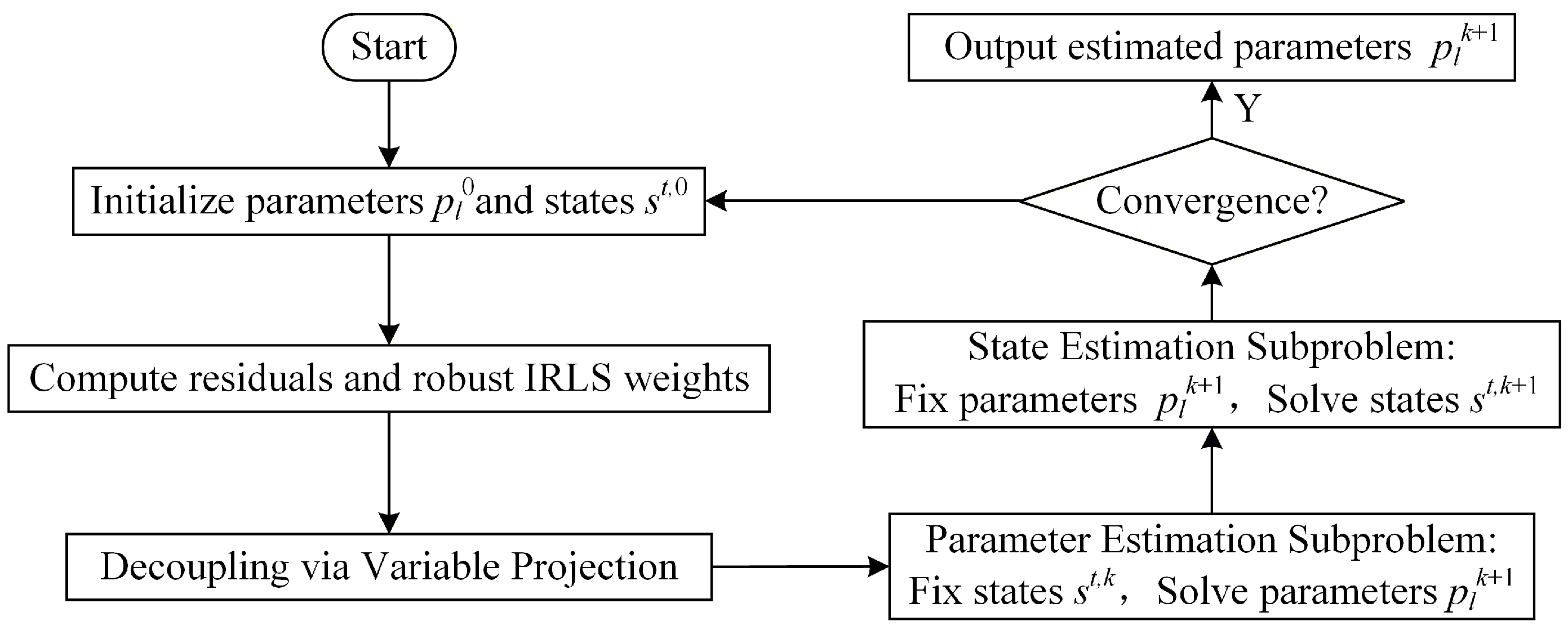
In summary, the proposed robust joint parameter and state estimation algorithm follows the iterative framework outlined in Figure 2. This framework combines IRLS to improve robustness with the VPM. It separates the parameter and state estimation steps, alternating between them until convergence is achieved. The detailed numerical steps of this framework are summarized in Algorithm 1.

Algorithm 1: Robust variable-projection estimation procedure.

Step 1: Initialize line parameters and multi-period states, i.e., set $p^0$ and $s^{t,0};$

Step 2: Compute residuals and robust IRLS weights using (6), and update the Huber weighting matrices according to (15);

Step 3: Form the linear least-squares parameter subproblem per (23), solve the normal equations, and obtain the updated parameters $p_l^{k+1};$

Step 4: For each time slice t, construct the Gauss–Newton state subproblem per (26), solve for $∆s^t$, and update $s^{t,k+1}=s^{t,k}+{\alpha }^t∆s^t$;

Step 5: If both the parameter and state changes satisfy the prescribed tolerances, go to Step 6; otherwise, set $k=k+1$ and return to Step 2;

Step 6: Terminate and output the final line-parameter estimate $p^k$.

3.7. Implementation Details and Computational Complexity

To improve the reproducibility of the proposed robust VPM-based estimation framework, the main implementation settings are summarized in this subsection.

In the Huber M-estimation procedure, the standardized residual is computed using the corresponding measurement standard deviation. In the numerical tests, the standard deviations are set as ${\sigma }_V= 0.005 \mathrm{p}.\mathrm{u}.$ for voltage magnitude measurements and ${\sigma }_P={\sigma }_Q=0.01 \mathrm{p}.\mathrm{u}.$ for active and reactive power measurements, consistent with the measurement noise settings in the case study. The Huber threshold $\delta$ is set to 1.345, which is a commonly used value that preserves high efficiency under Gaussian noise while reducing the influence of large residuals. For residuals whose absolute standardized value is smaller than $\delta$, the quadratic penalty is used; otherwise, the corresponding weight is reduced according to the Huber IRLS rule.

The line-parameter vector is initialized using the nominal parameter values from the network database. Specifically, the initial values of $R_l,X_l,G_{sh,l}$ and $B_{sh,l}$ are taken from the original IEEE 118-bus branch data. The state variables are initialized using available voltage magnitude and phase-angle measurements. For buses without direct voltage measurements, a flat-start initialization is adopted; namely, the voltage magnitude is set to 1.0 p.u. and the phase angle is set to 0, while the slack-bus angle is fixed as the reference angle. After each parameter update, the engineering constraints in Equation (17), including non-negative resistance and reactance constraints, are enforced by projection.

The outer VPM-IRLS iteration is terminated when both the relative parameter change and the relative objective-function change are smaller than the prescribed tolerances. In this paper, the relative tolerance for the parameter update is set to 10⁻⁵, and the relative tolerance for the objective-function change is set to 10⁻⁶. The maximum number of outer iterations is set to 50. In the state-estimation step, the Gauss–Newton update for each time period is stopped when the relative state correction is smaller than 10⁻⁵ or when the maximum number of inner iterations, set to 20, is reached.

A step-size control strategy is used to improve numerical stability. For both the parameter update and the state update, the initial step size is set to 1. If the robust objective function does not decrease after the update, a backtracking strategy is adopted, in which the step size is multiplied by 0.5 until the objective function decreases or the minimum step size, set to 10⁻⁴, is reached. This strategy prevents overly large corrections caused by nonlinear power-flow equations or temporary changes in robust weights.

For the PCG solver, a diagonal Jacobi preconditioner is used. In the parameter-estimation step, the preconditioner is constructed from the diagonal entries of the parameter normal matrix. In the state-estimation step, because the state-related matrix is block diagonal across time periods, the Jacobi preconditioner is constructed independently for each time-slice subproblem. The PCG iteration is stopped when the relative residual norm is smaller than 10⁻⁶ or when the maximum number of PCG iterations, set to 500, is reached. This avoids explicit matrix inversion and improves scalability for multi-period datasets.

The main computational cost of the proposed method consists of residual calculation, Jacobian construction, robust weight updating, and the solution of the parameter and state correction equations. Let T denote the number of time periods, $N_b$ the number of buses, $N_l$ the number of lines, m the average number of available measurements per time period, np the number of line-parameter variables, and ns the number of state variables per time period. Residual and weight updates require approximately O(Tm) operations. The construction of sparse Jacobian matrices also scales approximately linearly with the number of available measurements because each branch-flow measurement is only related to the parameters of one line and the states of its two terminal buses. In each PCG iteration, the dominant cost is matrix-vector multiplication, which is proportional to the number of nonzero elements in the corresponding sparse normal matrix. Therefore, the total cost can be approximately expressed as $O(Kout Tm + Kout Kpcg nnz(M\left)\right)$, where Kout is the number of outer VPM-IRLS iterations, Kpcg is the average number of PCG iterations, and $nnz\left(M\right)$ denotes the number of nonzero elements in the sparse coefficient matrix. Compared with direct matrix inversion or full factorization, whose the cost may grow cubically with the number of variables, the proposed PCG-based implementation is more suitable for large-scale multi-period parameter estimation.

The implementation parameters used in the simulations are summarized in

Table 3. Main implementation parameters of the proposed method.

Item	Setting Used in This Paper
Huber threshold $\delta$	1.345
Voltage magnitude standard deviation	${\sigma }_V=0.005 \mathrm{p}.\mathrm{u}.$
Branch active/reactive power standard deviation	${\sigma }_P={\sigma }_Q=0.01 \mathrm{p}.\mathrm{u}.$
Phase-angle standard deviation	${\sigma }_{\theta }=0.001 \mathrm{rad}$
Initial line parameters	Nominal IEEE 118-bus branch parameters
Initial voltage magnitude	Available measurements; otherwise, $1.0 \mathrm{p}.\mathrm{u}.$
Initial voltage angle	Available measurements; otherwise, 0
Slack-bus angle	Fixed as reference
Maximum outer VPM-IRLS iterations	50
Maximum Gauss–Newton iterations per time slice	20
Relative parameter-change tolerance	10−5
Relative objective-change tolerance	10−6
Step-size strategy	Backtracking, initial $\alpha =1,$ reduction factor = 0.5
Minimum step size	10−4
PCG preconditioner	Diagonal Jacobi preconditioner
PCG relative residual tolerance	10−6
Maximum PCG iterations	500

.

4. Case Study and Sustainability-Oriented Performance Assessment

To evaluate the performance of the robust joint parameter-estimation algorithm, hereafter referred to as “the proposed method,” simulation experiments are conducted on the standard IEEE 118-bus test system. Two representative benchmark methods, namely, the ideal weighted least squares method (WLS) and the conventional joint state-parameter estimation method (JSE), are used for comparison. This section first evaluates the proposed method in terms of parameter-estimation accuracy, error distribution characteristics, and robustness under gross measurement errors. Then, additional experiments are conducted to assess its implications for sustainable smart grid operation, including power-flow and loss evaluation as well as renewable-rich operating conditions.

4.1. Experimental Environment and Study Design

The full set of parameters for all $\pi$-equivalent circuits in the experimental case is derived from the data of the IEEE 118-bus system comprising 118 buses and 186 branches. It serves as the reference for subsequent error evaluation. To simulate data-driven analysis scenarios in modern smart grids, this case study constructs a time-series measurement dataset comprising $T=64$ time periods. At each time, uniform random perturbations within the range of $[-10\%, +10\%]$ are applied to the system’s base load, simulating natural intraday load fluctuations. Subsequently, an accurate power flow calculation is performed. This is to determine the true system states such as bus voltages and injected powers at each operating point. Finally, Gaussian white noise, modeled by a normal distribution, is added to these ground truth values to generate pseudo-measurement data. The noise standard deviations are set based on industry experience as follows:

• Bus-voltage magnitude: ${\sigma }_V= 0.005 \mathrm{p}.\mathrm{u}.$;
• Branch active/reactive power-flow measurements: ${\sigma }_P={\sigma }_Q=0.01 \mathrm{p}.\mathrm{u}.$

To evaluate the accuracy of the multidimensional estimation algorithm, several metrics are employed, such as Absolute Error (AE), Relative Error (RE), and Root Mean Square Error (RMSE). These metrics are defined by Equations (37)–(40).

$$AE\left(p_l\right)=\left|\Delta p_l\right|=\left|p_{l,est}-p_{l,true}\right|$$

(37)

$$RE\left(p_l\right)={\displaystyle \frac{\left|p_{l,est}-p_{l,true}\right|}{\left|p_{l,true}\right|}}\times 100\%$$

(38)

$$RMSAE\left(p_l\right)=\sqrt{{\displaystyle \frac{1}{L}}{\displaystyle \sum _{l=1}^L{\left[AE\left(p_l\right)\right]}^2}}$$

(39)

$$RMSRE\left(p_l\right)=\sqrt{{\displaystyle \frac{1}{L}}{\displaystyle \sum _{l=1}^L{\left[RE\left(p_l\right)\right]}^2}}$$

(40)

The detailed implementation parameters of the proposed method, including the Huber threshold, convergence tolerances, maximum iterations, initialization strategy, step-size rule, and PCG settings, are summarized in Table 3.

To provide a more comprehensive robustness evaluation, several additional benchmark methods are introduced in addition to WLS and conventional JSE. First, the weighted least absolute value method (WLAV) is used as a classical robust estimation method, where the weighted L1-norm of the measurement residuals is minimized to reduce the influence of gross errors. Second, the total least squares method (TLS) is considered to account for errors in both the measurement vector and the regression matrix. Third, an EKF-based state-parameter estimation method is included as a recursive benchmark, in which the line parameters are treated as slowly varying variables and updated together with the system states using time-series measurements. Finally, a robust M-estimation-based JSE method without variable projection, denoted as Huber-JSE, is added as an ablation benchmark. This method uses the same Huber loss and IRLS weight-updating rule as the proposed method but solves the original coupled state-parameter estimation problem directly, without the VPM-based projection and decomposition.

For fairness, all benchmark methods use the same measurement data, initial line parameters, measurement noise settings, gross-error locations, convergence tolerances, and evaluation metrics. The comparison is conducted under both Gaussian-noise conditions and 5% gross measurement errors. This design allows the robustness improvement brought by the Huber M-estimator and the additional benefit of the VPM-based decoupling strategy to be separately assessed.

4.2. Experimental Results and Analysis

4.2.1. Overall Estimation Accuracy

To evaluate the performance of the proposed method, the RMSEs of the four estimated parameters ($R_l,X_l,G_{sh,l},B_{sh,l}$) obtained by WLS, JSE, and the proposed method are compared in

Table 4. Comparison of estimation results.

Metric	Parameter	WLS	JSE	Proposed Method
RMSAE (×10−3)	$R_l$	0.15712	0.11085	0.08217
	$X_l$	0.32727	0.25279	0.17936
	$G_{sh}$	5.05265	3.56592	2.58251
	$B_{sh}$	2.25333	1.73275	1.39907
RMSRE (%)	$R_l$	1.36377	1.06311	0.8150
	$X_l$	0.15582	0.11261	0.0794
	$B_{sh}$	7.1376	6.3997	5.1453

Note: Since the true value of the shunt ground conductance $G_{sh}$ for most lines is zero, its relative error lacks mathematical significance and is therefore omitted from the table.

.

Table 4 shows that the proposed method outperforms the other methods in both RMSAE and RMSRE metrics. This superiority is most pronounced in the estimation of line reactance $X_l$, where it achieves an exceptionally low RMSRE of merely 0.0794%, which is significantly lower than the values recorded by the traditional JSE and WLS methods. This advantage stems from two key strengths of the proposed method. First, it effectively suppresses random noise by aggregating multi-period measurement data. Second, its robust M-estimation technique mitigates the negative effects of outliers. Furthermore, the algorithm excels in identifying the more challenging shunt branch parameters, achieving the lowest RMSAE among the three methods. These results demonstrate that the proposed method offers the highest overall estimation accuracy. It can reliably identify weakly observable parameters, including shunt branch parameters, from complex measurements.

From an operational perspective, more accurate line parameters can reduce model mismatch in state estimation and power-flow calculation, which is beneficial for the reliable and efficient operation of sustainable smart grids.

4.2.2. Error Distribution Characteristics

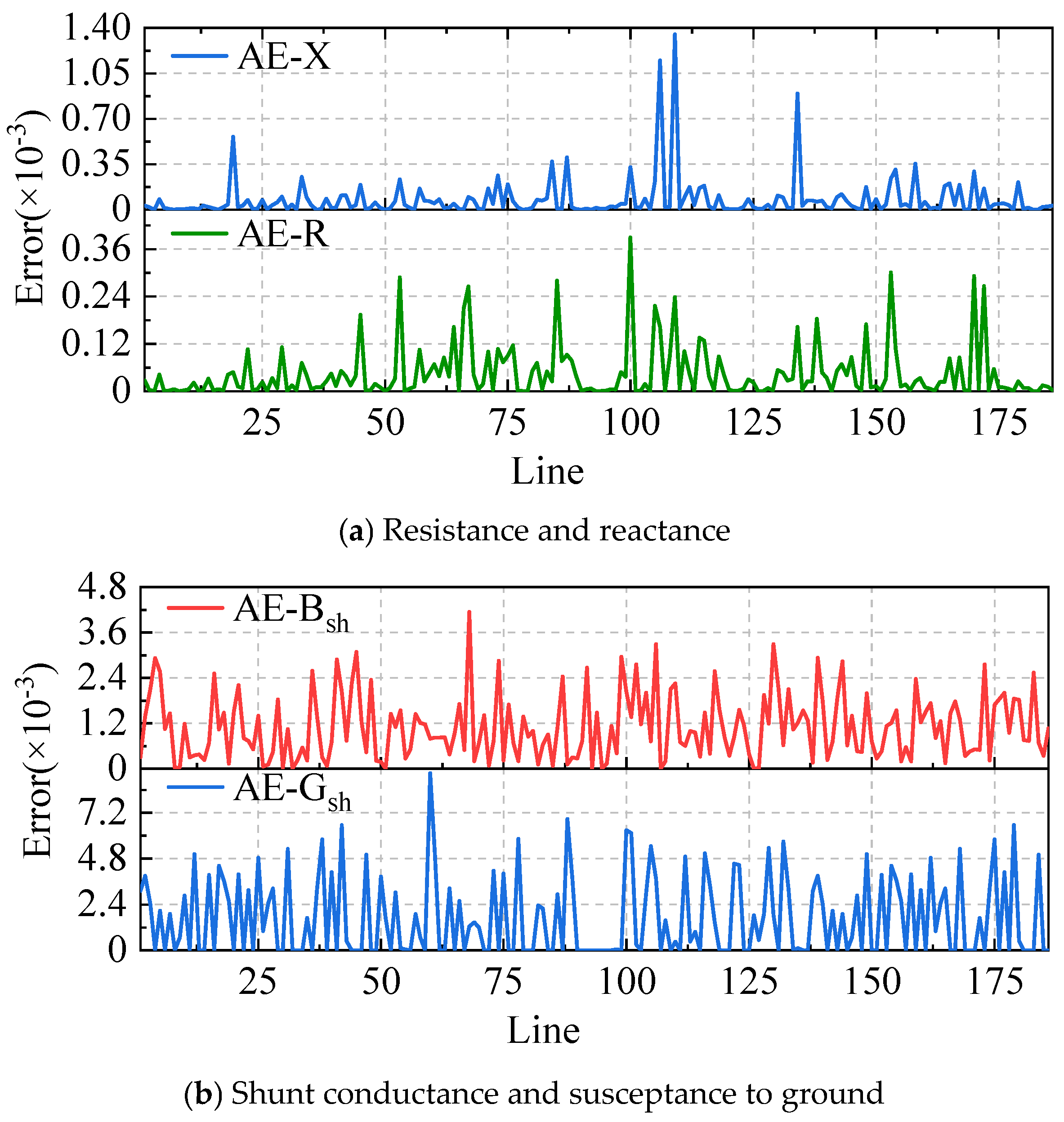
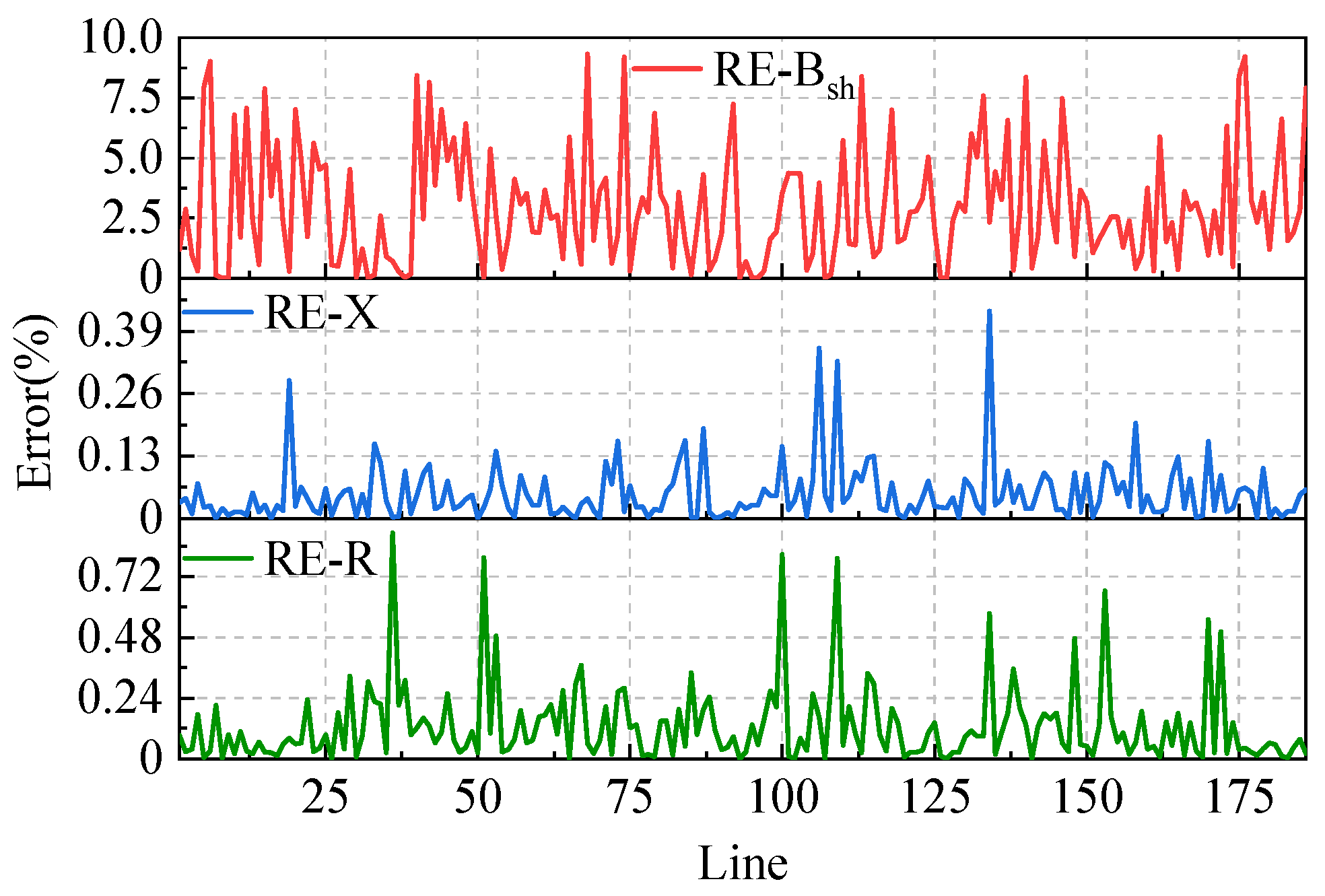
Figure 3 and Figure 4 illustrate the AE and RE of each line parameter using the proposed method.

Figure 3a illustrates the trend of AE for the series parameters $R_l$ and $X_l$. Overall, these errors remain low. The AE-R fluctuate within a narrow range, with most values concentrated below 0.12 × 10⁻³. Although the AE-X are slightly higher than the AE-R, the majority of lines still maintain error values within 0.36 × 10⁻³, with only a few lines showing peak errors. This demonstrates that the proposed method achieves a high accuracy and consistency in estimating series parameters.

Figure 3b shows the distribution of AE for $B_{sh}$ and $G_{sh}$. Compared to the series parameters, the AE for the shunt parameters is generally higher. Most lines exhibit AE-Gsh values between 2.4 × 10⁻³ and 4.8 × 10⁻³, with some lines reaching peak errors as high as 7.2 × 10⁻³. The AE-Bsh are primarily concentrated between 1.2 × 10⁻³ and 3.6 × 10⁻³. Although the estimation of shunt parameters presents greater challenges, the overall errors are contained within acceptable limits, and no systematic bias is observed.

It can be observed from the AE that the proposed method can well estimate four parameters. The series parameters show lower and more consistent error distributions. Although the shunt parameters exhibit slightly higher errors, the proposed method still achieves relatively accurate identification.

Figure 4 shows the distribution of RE for three types of parameters. Overall, the RE-R is the most tightly clustered, exhibiting minimal fluctuation and remaining close to the zero-error line. Its peak error does not exceed 0.13%. In contrast, the RE-X is slightly broader than that of reactance but generally stays within 0.24%. Among the shunt parameters, the RE-Bsh is noticeably wider, with greater fluctuations. For some lines, the peak error can reach approximately 7.5%, higher than that of the series parameters. This phenomenon aligns with theoretical expectations because the parameters of shunt branches inherently exhibit weak identifiability. This makes them more challenging to identify than series parameters.

Despite noticeable variations in error distributions across different parameters, the RE distributions for all parameters are centered around zero, showing no clear systematic overestimation or underestimation. This finding confirms the overall unbiasedness of the algorithm framework proposed in this paper.

The near-zero-centered error distributions indicate that the proposed method does not introduce obvious systematic bias. This property is important for long-term grid model maintenance, because biased line parameters may accumulate errors in repeated power-flow studies and operational assessments.

4.2.3. Robustness Verification

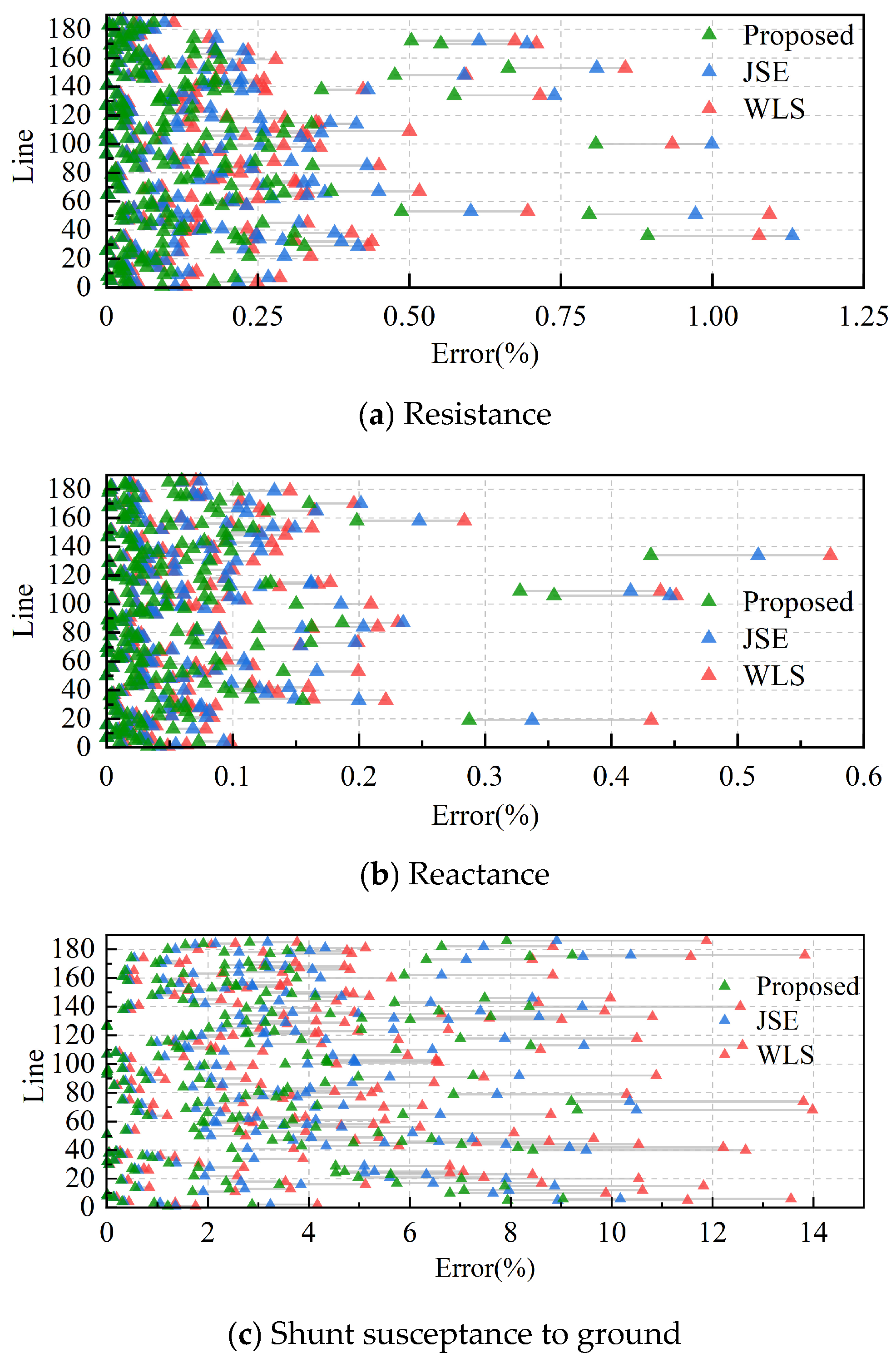
To assess the algorithm’s performance under non-ideal measurement conditions, we randomly selected 5% of the measurement data and doubled their true values for testing. Figure 5 compares the distribution of RE for each parameter across the three algorithms when the data is contaminated.

Table 5. Robustness comparison with additional benchmark methods under 5% gross measurement errors.

Method	RMSRE-${\mathit{R}}_{\mathit{l}}$ (%)	RMSRE-${\mathit{X}}_{\mathit{l}}$ (%)	RMSRE-${\mathit{B}}_{\mathit{s}\mathit{h}}$ (%)	Branch Flow RMSE (MW)	Voltage RMSE (p.u.)	Loss Error (%)
WLS	2.07372	0.23331	10.7936	1.6842	0.00482	2.4368
Conventional JSE	1.43420	0.15765	9.1326	1.1267	0.00341	1.6845
TLS	1.38653	0.14972	8.7241	1.0784	0.00328	1.5823
EKF-based method	1.26842	0.12693	7.5368	0.9526	0.00294	1.3617
WLAV	1.18476	0.11236	6.9842	0.8865	0.00271	1.2174
Huber-JSE without VPM	1.07184	0.09684	6.2459	0.8036	0.00243	1.0648
Proposed method	0.97719	0.08750	5.8536	0.7215	0.00216	0.9327

presents the overall RMSE, and

Table 6. Performance degradation rates under 5% gross errors.

Metric	Parameter	WLS Deg	JSE Deg	Proposed Method Deg
RMSAE (%)	$R_l$	40.00127	20.45106	12.30376
	$X_l$	44.00037	29.60560	17.55129
	$G_{sh}$	48.07913	39.71962	15.59994
	$B_{sh}$	53.86650	44.88472	16.23793
RMSRE (%)	$R_l$	52.05790	34.90608	19.90061
	$X_l$	49.73046	39.99645	10.20151
	$B_{sh}$	51.22170	42.70356	13.76596

quantifies the performance degradation rates from a clean environment to a contaminated one.

Figure 5 presents the performance under data contamination scenarios. As revealed by the results, the proposed robust VPM method maintains a distinct advantage in a harsh measurement environment with 5% bad data. It consistently outperforms the traditional WLS and JSE methods across all three key line parameters: resistance, reactance, and shunt admittance to ground. The advantage is clearly manifested in the error distributions. The proposed method consistently exhibits the narrowest range, the highest peak, and a distribution center closest to zero. In contrast, the comparison methods show significantly wider spreads and pronounced tails.

The comparison results in Table 5 show that the additional robust benchmark methods generally improve the estimation performance compared with WLS and conventional JSE under 5% gross measurement errors. TLS slightly reduces the estimation errors by considering errors in both the measurement vector and the regression matrix, but its improvement is limited because conventional TLS does not explicitly suppress gross outliers. The EKF-based method achieves better performance by recursively updating states and parameters using time-series measurements, but its accuracy is affected by linearization errors and the assumed parameter evolution model. WLAV provides a stronger robustness by minimizing the weighted L1-norm of residuals, leading to lower errors than TLS and EKF.

Among the benchmark methods, Huber-JSE without VPM achieves the closest performance to the proposed method. This is because it uses the same Huber M-estimator and IRLS-based weight-updating mechanism as the proposed framework. However, its errors are still higher than those of the proposed method, since it directly solves the original coupled state-parameter estimation problem without exploiting the variable-projection structure. In contrast, the proposed method achieves the lowest RMSREs for line resistance, reactance, and shunt susceptance, as well as the lowest branch-flow RMSE, voltage-magnitude RMSE, and active-power-loss error. These results confirm that the improvement of the proposed method comes not only from robust Huber weighting, but also from the VPM-based separation between time-invariant line parameters and time-varying operating states.

Table 6 quantifies the impact of bad data by presenting each algorithm’s performance degradation rate, measured as the RMSE growth from a pure Gaussian noise environment to a contaminated one.

The performance degradation rate analysis presented in Table 6 provides a dynamic assessment of each algorithm’s robustness. When the measurement environment shifts from clean to contaminated, the RMSE growth rates for all parameters in the proposed method are substantially lower. This demonstrates its superior robustness compared to the two comparison methods. Specifically, its degradation rate is generally less than one-third that of WLS and half that of JSE. These findings demonstrate that the proposed method effectively mitigates the impact of bad data, addressing the limitations of traditional methods. Note that the proposed method not only identifies the parameters but also estimates the system states at each time. In this framework, state estimation serves as an internal calibration step, providing an accurate physical context for the primary parameter identification. The experimental results demonstrate the overall effectiveness of this alternating iterative framework.

4.2.4. Monte Carlo Statistical Validation

To avoid drawing conclusions from a single random realization of measurement noise and gross errors, a Monte Carlo statistical validation was further conducted. Since the measurement dataset in this study contains random load perturbations, Gaussian measurement noise, and randomly distributed gross measurement errors, repeated trials are necessary to evaluate the statistical stability of different estimation methods.

In each Monte Carlo trial, the load perturbations, Gaussian measurement noise, and the locations of gross measurement errors were independently regenerated. The gross-error ratio was fixed at 5%, consistent with the robustness test in Section 4.2.3. To ensure a fair comparison, all compared methods were evaluated using exactly the same random measurement dataset in each trial. A total of 100 Monte Carlo trials were performed. For each method, the mean value, standard deviation, and 95% confidence interval of the RMSREs of line resistance, line reactance, and shunt susceptance were calculated.

The 95% confidence interval was computed as follows:

95% confidence interval = mean value ± 1.96 × standard deviation/square root of the number of Monte Carlo trials.

In this study, the number of Monte Carlo trials is 100. Therefore, the confidence interval reflects the uncertainty of the estimated mean performance over repeated random noise and gross-error realizations. The Monte Carlo statistical results are summarized in

Table 7. Monte Carlo statistical comparison under 5% gross measurement errors over 100 trials.

Method	RMSRE-${\mathit{R}}_{\mathit{l}}$ (%)	95%CI	RMSRE-${\mathit{X}}_{\mathit{l}}$ (%)	95%CI	RMSRE-${\mathit{B}}_{\mathit{s}\mathit{h}}$ (%)	95%CI
WLS	2.105 ± 0.214	[2.063, 2.147]	0.238 ± 0.026	[0.233, 0.243]	10.962 ± 0.894	[10.787, 11.137]
Conventional JSE	1.462 ± 0.156	[1.431, 1.493]	0.161 ± 0.018	[0.157, 0.165]	9.284 ± 0.742	[9.139, 9.429]
TLS	1.407 ± 0.148	[1.378, 1.436]	0.153 ± 0.017	[0.150, 0.156]	8.816 ± 0.703	[8.678, 8.954]
EKF based method	1.292 ± 0.132	[1.266, 1.318]	0.130 ± 0.015	[0.127, 0.133]	7.621 ± 0.618	[7.500, 7.742]
WLAV	1.207 ± 0.118	[1.184, 1.230]	0.115 ± 0.013	[0.112, 0.118]	7.063 ± 0.571	[6.951, 7.175]
Huber-JSE without VPM	1.089 ± 0.097	[1.070, 1.108]	0.099 ± 0.011	[0.097, 0.101]	6.318 ± 0.482	[6.224, 6.412]
Proposed method	0.991 ± 0.083	[0.975, 1.007]	0.089 ± 0.009	[0.087, 0.091]	5.918 ± 0.421	[5.836, 6.000]

.

As shown in Table 7, the proposed method achieves the lowest mean RMSREs among all compared methods. For line resistance, the mean RMSRE of the proposed method is 0.991%, which is lower than those of WLS, conventional JSE, TLS, EKF-based estimation, WLAV, and Huber-JSE without VPM. Similar improvements can be observed for line reactance and shunt susceptance. In particular, the mean RMSRE of line reactance is reduced to 0.089%, indicating that the proposed method maintains a high estimation accuracy under repeated random noise and gross-error conditions.

In addition to lower mean errors, the proposed method also shows smaller standard deviations than most benchmark methods. This indicates that the proposed method is not only more accurate but also more stable across different random realizations. Compared with WLS and conventional JSE, the confidence intervals of the proposed method are much narrower and located at lower error levels. This confirms that the improved performance of the proposed method is not caused by a particular random experiment, but is maintained consistently over repeated trials.

To further examine whether the improvement is statistically significant, paired statistical tests were conducted between the proposed method and each benchmark method. Since all methods used the same random measurement dataset in each Monte Carlo trial, the paired t-test was adopted. The p-values are summarized in

Table 8. Paired t-test results between the proposed method and benchmark methods.

Comparison	${\mathit{R}}_{\mathit{l}}$-Value	${\mathit{X}}_{\mathit{l}}$-Value	${\mathit{B}}_{\mathit{s}\mathit{h}}$-Value
Proposed vs. WLS	<0.001	<0.001	<0.001
Proposed vs. Conventional JSE	<0.001	<0.001	<0.001
Proposed vs. TLS	<0.001	<0.001	<0.001
Proposed vs. EKF-based method	<0.001	<0.001	<0.001
Proposed vs. WLAV	<0.01	<0.01	<0.01
Proposed vs. Huber-JSE without VPM	<0.05	<0.05	<0.05

.

The statistical test results in Table 8 show that the proposed method achieves statistically significant improvements over WLS, conventional JSE, TLS, EKF-based estimation, WLAV, and Huber-JSE without VPM. The differences between the proposed method and WLS, conventional JSE, TLS, and EKF-based estimation are significant at the 0.001 level for all three parameters. Compared with WLAV, the proposed method is significant at the 0.01 level. Compared with Huber-JSE without VPM, the proposed method is significant at the 0.05 level, indicating that the VPM-based decomposition further improves estimation accuracy beyond the robust Huber weighting mechanism.

Overall, the Monte Carlo statistical validation demonstrates that the proposed robust VPM framework consistently outperforms the benchmark methods under repeated random noise and gross-error conditions. Therefore, the robustness advantage of the proposed method is statistically supported rather than being based on a single-run result.

4.2.5. Sensitivity Analysis Under Different Bad-Data Scenarios

To further evaluate the robustness of the proposed method beyond a single gross-error setting, additional sensitivity tests were conducted under different contamination ratios, outlier magnitudes, and outlier-location patterns. In the original robustness test, 5% of the measurements were randomly selected and multiplied by a factor of 2.0. Although this setting can represent a typical gross-error scenario, it does not fully reflect the diversity of possible bad-data conditions in practical measurement systems. Therefore, this subsection extends the robustness analysis by considering three aspects: the percentage of contaminated measurements, the magnitude of outliers, and the spatial or measurement-type location of outliers.

Let $\gamma$ denote the gross-error contamination ratio and $\alpha$ denote the outlier magnitude factor. For a selected bad-data measurement $z_i$, the corrupted value is generated as

$$z_i^{bad}=\alpha z_i,i\in {\Omega }_{bad}$$

where ${\Omega }_{bad}$ is the set of contaminated measurements. Unless otherwise specified, the Gaussian measurement noise, initial line parameters, convergence tolerances, and evaluation metrics are kept the same as those used in the previous experiments. For a fair comparison, all compared methods use exactly the same corrupted measurement datasets under each bad-data scenario.

First, the contamination ratio $\gamma$ was varied from 1% to 20%, while the outlier magnitude factor was fixed at $\alpha =2.0$. The selected contamination ratios were 1%, 3%, 5%, 10%, and 20%. The results are summarized in

Table 9. Robustness comparison under different gross-error contamination ratios.

Contamination Ratio	Method	RMSRE-${\mathit{R}}_{\mathit{l}}$ (%)	RMSRE-${\mathit{X}}_{\mathit{l}}$ (%)	RMSRE-${\mathit{B}}_{\mathit{s}\mathit{h}}$ (%)
1%	WLS	1.52034	0.17562	7.8421
	Conventional JSE	1.15547	0.12584	6.9824
	Huber-JSE without VPM	0.90536	0.08342	5.5627
	Proposed method	0.84218	0.07691	5.2365
3%	WLS	1.78591	0.20477	9.1284
	Conventional JSE	1.28173	0.14136	7.8530
	Huber-JSE without VPM	0.98642	0.09077	5.9024
	Proposed method	0.91085	0.08264	5.5472
5%	WLS	2.07372	0.23331	10.7936
	Conventional JSE	1.43420	0.15765	9.1326
	Huber-JSE without VPM	1.07184	0.09684	6.2459
	Proposed method	0.97719	0.08750	5.8536
10%	WLS	2.76548	0.31592	14.3285
	Conventional JSE	1.87264	0.21046	11.6842
	Huber-JSE without VPM	1.31278	0.12163	7.2156
	Proposed method	1.17653	0.10827	6.7214
20%	WLS	4.18956	0.48237	21.7862
	Conventional JSE	2.84631	0.32684	17.9246
	Huber-JSE without VPM	1.87429	0.17836	9.8427
	Proposed method	1.60482	0.15194	8.7593

.

As shown in Table 9, the RMSREs of all methods increase as the contamination ratio increases from 1% to 20%. However, the proposed method consistently achieves the lowest RMSREs for resistance, reactance, and shunt susceptance under all contamination levels. For example, at the 20% contamination ratio, the proposed method reduces the RMSREs of $R_l$, $X_l$, and $B_{sh}$ to 1.60482%, 0.15194%, and 8.7593%, respectively, which are much lower than those of WLS and conventional JSE. This confirms that the proposed method maintains a stable robustness even under severe contamination.

Second, the influence of different outlier magnitudes was examined. In this test, the contamination ratio was fixed at 5%, while the outlier magnitude factor $\alpha$ was varied as 1.5, 2.0, 3.0, and 5.0. The results are presented in

Table 10. Robustness comparison under different outlier magnitude factors.

Outlier Magnitude Factor	Method	RMSRE-${\mathit{R}}_{\mathit{l}}$ (%)	RMSRE-${\mathit{X}}_{\mathit{l}}$ (%)	RMSRE-${\mathit{B}}_{\mathit{s}\mathit{h}}$ (%)
1.5×	WLS	1.76125	0.19843	9.1025
	Conventional JSE	1.24589	0.13674	7.8456
	Huber-JSE without VPM	0.94837	0.08692	5.7243
	Proposed method	0.88674	0.08034	5.3821
2.0×	WLS	2.07372	0.23331	10.7936
	Conventional JSE	1.43420	0.15765	9.1326
	Huber-JSE without VPM	1.07184	0.09684	6.2459
	Proposed method	0.97719	0.08750	5.8536
3.0×	WLS	2.68491	0.30478	14.2157
	Conventional JSE	1.84237	0.20564	11.4628
	Huber-JSE without VPM	1.28764	0.11893	7.1046
	Proposed method	1.14186	0.10472	6.5849
5.0×	WLS	3.89273	0.45196	20.6384
	Conventional JSE	2.61528	0.29837	16.4027
	Huber-JSE without VPM	1.73895	0.16428	9.3621
	Proposed method	1.48673	0.13965	8.2754

.

Table 10 shows that larger outlier magnitudes lead to higher estimation errors for all methods. This is expected because the contaminated measurements deviate more severely from the true measurement values. Nevertheless, the proposed method remains the most accurate under all tested outlier magnitudes. Compared with WLS and conventional JSE, the proposed method shows a much slower error growth rate as the outlier magnitude increases. For example, when the outlier magnitude factor increases from 1.5 to 5.0, the RMSRE-$R_l$ of WLS increases from 1.76125% to 3.89273%, whereas that of the proposed method increases from 0.88674% to 1.48673%. This confirms that the proposed robust VPM framework is not only effective for the original doubling-error case but also remains effective under more severe gross-error amplitudes.

Third, different outlier-location patterns were considered. In this test, the contamination ratio was fixed at 5%, and the outlier magnitude factor was fixed at 2.0. Five representative location patterns were tested: uniformly random contamination, contamination concentrated on branch power-flow measurements, contamination concentrated on bus-related measurements, spatially clustered contamination around selected local network areas, and contamination assigned to high-leverage branches. The results are summarized in

Table 11. Robustness comparison under different outlier-location patterns.

Outlier-Location Pattern	Method	RMSRE-${\mathit{R}}_{\mathit{l}}$ (%)	RMSRE-${\mathit{X}}_{\mathit{l}}$ (%)	RMSRE-${\mathit{B}}_{\mathit{s}\mathit{h}}$ (%)
Random contamination	WLS	2.07372	0.23331	10.7936
	Conventional JSE	1.43420	0.15765	9.1326
	Huber-JSE without VPM	1.07184	0.09684	6.2459
	Proposed method	0.97719	0.08750	5.8536
Branch-flow concentrated	WLS	2.31485	0.26214	12.0873
	Conventional JSE	1.59237	0.17658	10.2459
	Huber-JSE without VPM	1.15264	0.10593	6.7046
	Proposed method	1.03158	0.09524	6.2138
Bus-measurement concentrated	WLS	1.90248	0.21975	9.8472
	Conventional JSE	1.33516	0.14982	8.5634
	Huber-JSE without VPM	1.00685	0.09317	6.0845
	Proposed method	0.92641	0.08436	5.7129
Spatially clustered	WLS	2.48672	0.28154	13.2056
	Conventional JSE	1.72143	0.19431	10.9638
	Huber-JSE without VPM	1.25376	0.11584	7.0249
	Proposed method	1.10735	0.10192	6.4537
High-leverage branches	WLS	2.73156	0.30982	14.6721
	Conventional JSE	1.94305	0.21846	12.0863
	Huber-JSE without VPM	1.35948	0.12751	7.6932
	Proposed method	1.19684	0.11168	7.0215

.

The results in Table 11 further demonstrate that the location of gross errors has a clear impact on estimation accuracy. Contamination concentrated on branch power-flow measurements generally causes larger errors than contamination concentrated on bus-related measurements, because branch power-flow measurements are directly related to the line-parameter equations. Spatially clustered outliers and high-leverage branch outliers are more challenging than uniformly random outliers, since they may introduce locally biased information into the estimation process. Even under these difficult conditions, the proposed method still achieves the lowest RMSREs among all compared methods. This result indicates that the proposed method does not rely on a specific random outlier distribution and can maintain a stable estimation performance under different bad-data locations.

Overall, the sensitivity analysis confirms that the robustness advantage of the proposed method is not limited to the original 5% gross-error scenario with doubled selected measurements. Instead, the proposed method consistently outperforms WLS, conventional JSE, and Huber-JSE without VPM under different contamination ratios, different outlier magnitudes, and different outlier-location patterns. These results provide additional evidence that the combination of Huber-IRLS-based robust weighting and VPM-based state-parameter decomposition is effective for transmission-line parameter estimation under diverse bad-data conditions.

4.2.6. Impact on Sustainable Smart Grid Operation

Accurate line parameters are not only important for parameter identification itself, but also directly affect downstream model-based grid analysis, such as the power-flow calculation, voltage assessment, active power loss evaluation, and operational security assessment. To further investigate the practical implications of the proposed method for sustainable smart grid operation, the line parameters estimated by WLS, JSE, and the proposed method are respectively substituted into the network model, and power-flow calculations are performed under the same operating conditions.

The results obtained using the true line parameters are regarded as the reference. The calculated branch active power flows, bus-voltage magnitudes, and active power losses obtained using different estimated parameter sets are then compared with the reference values. Three indicators are adopted: branch active power flow RMSE, bus-voltage magnitude RMSE, and active power loss estimation error. These indicators are defined as follows:

$$E_P=\sqrt{{\displaystyle \frac{1}{N_{l}T}}{\displaystyle \sum _{t=1}^T}{\displaystyle \sum _{l=1}^{N_l}}{\left(P_{l,t}^{est}-P_{l,t}^{true}\right)}^2}$$

(41)

$${\mathrm{E}}_V=\sqrt{{\displaystyle \frac{1}{N_{b}T}}{\displaystyle \sum _{t=1}^T}{\displaystyle \sum _{i=1}^{N_b}}{\left(V_{i,t}^{est}-V_{i,t}^{true}\right)}^2}$$

(42)

$$E_{loss}={\displaystyle \frac{|P_{loss}^{est}-P_{loss}^{true}|}{P_{loss}^{true}}}\times 100\%$$

(43)

where $N_l$ is the number of transmission lines, $N_b$ is the number of buses, and $T$ is the number of time periods. $P_{l,t}^{est}$ and $P_{l,t}^{true}$ denote the estimated and reference active power flows of line $l$ at time $t$, respectively. $V_{i,t}^{est}$ and $V_{i,t}^{true}$ denote the estimated and reference voltage magnitudes of bus $i$ at time $t$, respectively. $P_{loss}^{est}$ and $P_{loss}^{true}$ denote the total active power losses calculated using the estimated and true line parameters, respectively.

The comparison results are shown in

Table 12. Impact of parameter estimation on power-flow, voltage-magnitude, and active-power-loss evaluation.

Method	Branch Flow RMSE (MW)	Voltage Magnitude RMSE (p.u.)	Active Power Loss Error (%)
WLS	1.6842	0.00482	2.4368
JSE	1.1267	0.00341	1.6845
Proposed Method	0.7215	0.00216	0.9327

.

As shown in Table 12, the proposed method achieves the lowest branch flow RMSE, voltage magnitude RMSE, and active power loss estimation error among the three compared methods. Compared with WLS, the proposed method reduces the branch flow RMSE from 1.6842 MW to 0.7215 MW, the voltage magnitude RMSE from 0.00482 p.u. to 0.00216 p.u., and the active power loss error from 2.4368% to 0.9327%. Compared with JSE, the proposed method also achieves clear reductions in all three downstream evaluation indicators. This result indicates that the proposed robust parameter-estimation framework can reduce model mismatch not only at the parameter level but also in power-flow calculation, voltage assessment, and loss evaluation.

4.2.7. Performance Under Renewable-Rich Operating Conditions

With the increasing integration of renewable energy resources, power systems are subject to stronger operating fluctuations and higher uncertainty. These variations increase the diversity of operating states and place higher requirements on the accuracy and robustness of grid model calibration. To examine the adaptability of the proposed method under renewable-rich operating conditions, several generation buses in the IEEE 118-bus system are selected as renewable injection buses. Their active power outputs are assumed to fluctuate around the base operating points. The specific settings of the experimental data are provided in Reference [30].

The renewable power injection at time t is modeled as

$$P_{ren,t}=P_{ren,0}(1+{ϵ}_t)$$

(44)

where $P_{ren,0}$ is the base renewable power output, and ${ϵ}_t$ is a random fluctuation factor. In this study, two renewable fluctuation levels are considered:

$${\epsilon }_t~U(-20\%,20\%)$$

and

$${\epsilon }_t~U(-40\%,40\%)$$

The first case represents a moderate renewable fluctuation, while the second case represents a high renewable fluctuation. For each renewable-rich scenario, multi-period power-flow calculations are performed to generate the corresponding pseudo-measurement data. The same Gaussian noise setting is used, and 5% of the measurements are randomly selected and corrupted using the same gross-error rule as in the robustness test. WLS, JSE, and the proposed method are used to estimate the line parameters under each scenario.

The estimation performance under renewable-rich operating conditions is summarized in

Table 13. Estimation performance under renewable-rich operating conditions.

Scenario	Method	RMSRE-${\mathit{R}}_{\mathit{l}}$ (%)	RMSRE-${\mathit{X}}_{\mathit{l}}$ (%)	RMSRE-${\mathit{B}}_{\mathit{s}\mathit{h}}$ (%)	Loss Error (%)
Base	WLS	2.07372	0.23331	10.7936	2.4368
Base	JSE	1.43420	0.15765	9.1326	1.6845
Base	Proposed Method	0.97719	0.08750	5.8536	0.9327
R20	WLS	2.28654	0.25284	11.3682	2.6841
R20	JSE	1.57483	0.17192	9.6984	1.8627
R20	Proposed Method	1.05642	0.09386	6.1375	1.0184
R40	WLS	2.61278	0.28495	12.2547	3.0876
R40	JSE	1.80236	0.19384	10.5412	2.1374
R40	Proposed Method	1.17965	0.10341	6.4918	1.1462

Note: R20 and R40 denote ±20% and ±40% renewable power fluctuation scenarios, respectively. The base case in this table denotes the non-renewable-fluctuation case under the same 5% gross-error setting as Section 4.2.3, rather than the clean Gaussian-noise base case in Table 4.

.

As shown in Table 13, the estimation errors of all methods increase as the renewable fluctuation level becomes higher. For example, when the renewable fluctuation level increases from the base case to the ±40% scenario, the RMSRE-R of WLS increases from 2.07372% to 2.61278%, while that of JSE increases from 1.43420% to 1.80236%. In contrast, the RMSRE-R of the proposed method only increases from 0.97719% to 1.17965%, indicating a slower degradation rate under highly variable operating conditions.

A similar trend can also be observed for line reactance and shunt susceptance to ground. Under the ±40% renewable fluctuation scenario, the proposed method achieves RMSRE-X of 0.10341% and RMSRE-Bsh of 6.4918%, both of which are lower than those of WLS and JSE. In addition, the active power loss error of the proposed method is only 1.1462%, while those of WLS and JSE reach 3.0876% and 2.1374%, respectively. These results demonstrate that the proposed method maintains a better estimation accuracy and downstream loss-evaluation performance under renewable-rich operating conditions.

4.2.8. Cross-System Validation and Computational Scalability

To further evaluate the applicability of the proposed method beyond the IEEE 118-bus system, an additional IEEE 30-bus test system was introduced as a cross-system validation case. The original case study was conducted on the IEEE 118-bus system with 118 buses and 186 transmission lines, using $T=64$ operating periods and load perturbations uniformly sampled within $[-10\%,+10\%].$ To make the additional case comparable with the original one, the same data-generation procedure, noise settings, robust estimation parameters, and convergence criteria were adopted for the IEEE 30-bus system. Specifically, 64 operating snapshots were generated through AC power-flow calculations after applying random load perturbations. Gaussian noise was then added to the simulated measurements using the same noise settings as the base-case experiment. No gross measurement errors were introduced in this cross-system accuracy test.

The IEEE 30-bus system is smaller than the IEEE 118-bus system, but it has a different network topology, line-parameter distribution, and measurement configuration. Therefore, this additional case is mainly used to verify whether the proposed method is tailored only to the IEEE 118-bus system or can maintain stable performance under another benchmark network. The main system settings are summarized in

Table 14. Test-system settings for cross-system validation.

Test System	Number of Buses	Number of Branches	Number of Estimated Line Parameters	Time Periods	Load Perturbation
IEEE 30-bus	30	41	164	64	$[-10\%,+10\%]$
IEEE 118-bus	118	186	744	64	$[-10\%,+10\%]$

.

For each transmission line, four parameters, namely, $R_l,X_l,G_{sh,l}$, and $B_{sh,l}$, were estimated. Therefore, the total number of line-parameter variables is ${4N}_l$, where $N_l$ is the number of transmission lines. The same three methods, namely, WLS, JSE, and the proposed robust VPM method, were compared under the same measurement conditions.

The estimation results of the IEEE 30-bus system are shown in

Table 15. Cross-system comparison of parameter-estimation accuracy.

Test System	Method	RMSRE-${\mathit{R}}_{\mathit{l}}$ (%)	RMSRE-${\mathit{X}}_{\mathit{l}}$ (%)	RMSRE-${\mathit{B}}_{\mathit{s}\mathit{h}}$ (%)
IEEE 30-bus	WLS	0.40611	0.25261	5.56763
	JSE	0.35160	0.21519	4.81013
	Proposed method	0.27256	0.18712	3.78753
IEEE 118-bus	WLS	1.36377	0.15582	7.1376
	JSE	1.06311	0.11261	6.3997
	Proposed method	0.8150	0.0794	5.1453

. The original IEEE 118-bus results are also listed for comparison. Since the true value of $G_{sh,l}$ is zero or close to zero for many lines, its relative error may not be mathematically meaningful. Therefore, the relative-error comparison mainly focuses on $R_l,X_l$, and $B_{sh,l}$.

As shown in Table 15, the proposed method achieves the lowest estimation errors in both the IEEE 30-bus and IEEE 118-bus systems. In the IEEE 118-bus system, the proposed method reduces the RMSRE of $R_l,X_l$, and $B_{sh,l}$ to 0.8150%, 0.0794%, and 5.1453%, respectively. These values are lower than those obtained by WLS and conventional JSE. The additional IEEE 30-bus results show the same trend: the proposed method obtains lower errors than the two comparison methods under a different network topology. This confirms that the improvement is not limited to a single IEEE 118-bus test system.

In addition to the cross-system comparison, the scalability with respect to the number of time periods was examined on the IEEE 118-bus system. The number of operating periods was varied as $T=\mathrm{32,64,128,256}$ while the network topology, measurement types, noise settings, and convergence criteria were kept unchanged. The results are summarized in

Table 16. Computational scalability with respect to the number of time periods on the IEEE 118-bus system.

Time Periods (T)	Number of Estimated Line Parameters	Relative Parameter-Change Tolerance	Outer Iterations	Average PCG Iterations	Normalized CPU Time	Con-Verged
32	744	10−5	18	18.6	0.53	Yes
64			23	20.4	1.00	Yes
128			29	22.7	2.12	Yes
256			37	25.1	4.46	Yes

The CPU time is normalized by the runtime of the $T=64$ case to reduce hardware dependence.

.

Table 16 shows that the proposed method remains numerically stable as the number of time periods increases. The number of line-parameter variables remains unchanged because the line parameters are time-invariant, whereas the number of state variables and measurements increases with $T$. The CPU time increases with the number of time periods, but the convergence behavior remains stable. This result is consistent with the block structure of the proposed method: the state-estimation subproblems are separated by time period, while the parameter-estimation step aggregates multi-period information through sparse Jacobian matrices.

Overall, the additional IEEE 30-bus case demonstrates the cross-system applicability of the proposed method, while the time-period scalability test on the IEEE 118-bus system verifies its computational stability for larger multi-period datasets. These results further support the applicability of the proposed robust VPM framework to transmission-line parameter estimation problems with different network sizes and data volumes.

5. Conclusions

This paper proposed a robust data-driven transmission-line parameter estimation framework for the reliable and sustainable smart grid operation. By combining the variable projection method with Huber M-estimation, the proposed framework decomposes the high-dimensional joint estimation problem into parameter-identification and operating-state calibration subproblems, while adaptively reducing the influence of abnormal measurements through IRLS.

Case studies on the IEEE 118-bus system demonstrated that the proposed method achieves lower RMSAE and RMSRE than conventional WLS and JSE methods. Under gross-error contamination, the proposed method also exhibited significantly smaller performance degradation, confirming its robustness against imperfect measurement data. In addition, the proposed method produced a lower branch-flow RMSE, voltage-magnitude RMSE, and active-power-loss estimation error in downstream power-flow evaluation. The renewable-rich operating scenarios further verified that the proposed method maintains a better estimation accuracy and loss-evaluation performance under variable operating conditions.

From the perspective of sustainable smart grid operation, accurate and robust transmission-line parameter estimation can reduce model mismatch in state estimation, power-flow calculation, loss evaluation, and security assessment. Therefore, the proposed method provides a practical model-calibration tool for data-driven smart grids, especially under variable operating conditions and poor-quality measurements. Future work will further investigate online model updating using real field measurements and extend the proposed framework to uncertainty-aware operation in large-scale renewable-rich power systems.

References

1. Khalid, M. Smart grids and renewable energy systems: Perspectives and grid integration challenges. Energy Strategy Rev. 2024, 51, 101299. [Google Scholar] [CrossRef]
2. Eltigani, D.; Masri, S. Challenges of integrating renewable energy sources to smart grids: A review. Renew. Sustain. Energy Rev. 2015, 52, 770–780. [Google Scholar] [CrossRef]
3. Kroposki, B.; Zhang, Y.; Gevorgian, V.; Denholm, P.; Hodge, B.-M.; Hannegan, B. Achieving a 100% renewable grid: Operating electric power systems with extremely high levels of variable renewable energy. IEEE Power Energy Mag. 2017, 15, 61–73. [Google Scholar] [CrossRef]
4. Jiang, X.; Zhou, C.; Pan, Q.; Wang, L.; Wu, B.; Xu, Y.; Chen, K.; Fu, L. A multi–task learning based line parameter identification method for medium–voltage distribution network. Front. Energy Res. 2024, 12, 1485369. [Google Scholar] [CrossRef]
5. Zhang, J.; Wang, Y.; Weng, Y.; Zhang, N. Topology identification and line parameter estimation for non–PMU distribution network: A numerical method. IEEE Trans. Smart Grid 2020, 11, 4440–4453. [Google Scholar] [CrossRef]
6. Liu, J.; Chen, L.; Zhang, Z. Measurability estimation of static parameters in distribution network considering measurement error influence. Power Syst. Technol. 2020, 44, 1481–1487. [Google Scholar]
7. Brouillon, J.-S.; Moffat, K.; Dörfler, F.; Ferrari-Trecate, G. Power grid parameter estimation without phase measurements: Theory and empirical validation. Electr. Power Syst. Res. 2024, 235, 110709. [Google Scholar] [CrossRef]
8. Dobakhshari, A.S.; Abdolmaleki, M.; Terzija, V.; Azizi, S. Online non–iterative estimation of transmission line and transformer parameters by SCADA data. IEEE Trans. Power Syst. 2021, 36, 2632–2641. [Google Scholar] [CrossRef]
9. De Moraes, V.C.; de Sousa, L.L.S.; de Melo, I.D.; Duque, C.A.; de Souza, M.A.; de Oliveira, B.C. Transmission line parameters estimation using synchronised phasor measurements. In Proceedings of the 2024 IEEE Power & Energy Society General Meeting, Seattle, WA, USA, 21–25 July 2024; pp. 1–5. [Google Scholar]
10. Yao, R.; Huang, H.; Peng, F.; Guo, W. Transmission line parameter identification method based on synchronized phasor measurement unit. Autom. Technol. Appl. 2019, 38, 101–103+109. [Google Scholar]
11. Li, Q.; Xiang, F.; Yan, W.; Lu, J.; Yu, J.; Chen, J.; Li, S. Independent line parameter estimation method based on SCADA and PMU multi–time section measurement information. Power Syst. Technol. 2011, 35, 105–109. [Google Scholar]
12. Wang, Q.; Wu, Y.; Ci, W.; Cao, J.; Zhang, Y. Research on line parameter identification based on SCADA and WAMS. Shandong Electr. Power 2017, 44, 42–46. [Google Scholar]
13. Zhang, J.; Lei, J.; He, Y.; Wu, P.; Yu, J.; Xiang, M.; Ren, L. Online identification method for transmission line parameters based on PMU error correction. Power Syst. Prot. Control 2022, 50, 130–137. [Google Scholar]
14. Xue, A.; Xu, J.; Xu, F.; You, H.; Joe, H.C.; Bi, T. Calibration method for PMU phase angle difference at both ends of transmission line under unknown parameters. Autom. Electr. Power Syst. 2019, 43, 129–135. [Google Scholar]
15. Xue, A.; Xu, F.; Martin, K.E.; Xu, J.; You, H.; Bi, T. Linear approximations for the influence of phasor angle difference errors on line parameter calculation. IEEE Trans. Power Syst. 2019, 34, 3455–3464. [Google Scholar] [CrossRef]
16. Li, J.; Sun, J.; Li, C. Synchrophasor data analytics: Transmission line parameters online estimation for energy management. IEEE Trans. Eng. Manag. 2019, 66, 671–681. [Google Scholar] [CrossRef]
17. Varghese, A.C.; Pal, A.; Dasarathy, G. Transmission line parameter estimation under non–Gaussian measurement noise. IEEE Trans. Power Syst. 2023, 38, 3147–3162. [Google Scholar] [CrossRef]
18. Ribeiro Pereira, R.F.; de Albuquerque, F.P.; Bartocci Liboni, L.H.; Costa, E.C.M.; de Oliveira, M.C. Impedance parameters estimation of transmission lines by an extended Kalman filter–based algorithm. IEEE Trans. Instrum. Meas. 2022, 71, 9003610-1–9003610-10. [Google Scholar]
19. Bian, X.; Li, X.R.; Chen, H.; Gan, D.; Qiu, J. Joint estimation of state and parameter with synchrophasors—Part I: State tracking. IEEE Trans. Power Syst. 2011, 26, 1196–1208. [Google Scholar] [CrossRef]
20. Bian, X.; Li, X.R.; Chen, H.; Gan, D.; Qiu, J. Joint estimation of state and parameter with synchrophasors—Part II: Parameter tracking. IEEE Trans. Power Syst. 2011, 26, 1209–1220. [Google Scholar] [CrossRef]
21. Costa, E.C.M.D. Phasor Measurement Unit-Driven Estimation of Transmission Line Parameters Using Variable Noise Model. Energies 2024, 17, 3587. [Google Scholar] [CrossRef]
22. Moghanian, M.; Dobakhshari, A.S. Accurate Kalman filter based estimation of transmission line parameters utilizing synchronized phasor measurements. Electr. Power Syst. Res. 2024, 230, 110218. [Google Scholar] [CrossRef]
23. Pattanaik, V.; Malika, B.K.; Panda, S.; Rout, P.K.; Sahu, B.K.; Samanta, I.S.; Bajaj, M.; Blazek, V.; Prokop, L. A critical review on phasor measurement units installation planning and application in smart grid environment. Results Eng. 2024, 24, 103559. [Google Scholar] [CrossRef]
24. Fiorucci, E.; Fioravanti, A.; Mari, S.; Luiso, M.; Ciancetta, F. Driving Sustainable Development with PMU Systems in Distribution Grids. Sustainability 2025, 17, 5280. [Google Scholar] [CrossRef]
25. Mathiesen, B.V.; Lund, H.; Connolly, D.; Wenzel, H.; Østergaard, P.A.; Möller, B.; Nielsen, S.; Ridjan, I.; Karnøe, P.; Sperling, K.; et al. Smart Energy Systems for coherent 100% renewable energy and transport solutions. Appl. Energy 2015, 145, 139–154. [Google Scholar] [CrossRef]
26. Wehenkel, A.; Mukhopadhyay, A.; Le Boudec, J.-Y.; Paolone, M. Parameter estimation of three-phase untransposed short transmission lines from synchrophasor measurements. IEEE Trans. Instrum. Meas. 2020, 69, 6143–6154. [Google Scholar] [CrossRef]
27. Khalili, R.; Abur, A. Transmission line parameter error identification and estimation in three-phase networks. IEEE Trans. Power Syst. 2022, 37, 2271–2282. [Google Scholar] [CrossRef]
28. Gerez, C.; Angelos, E.W.S.; Albuquerque, F.P.; Da Costa, E.C.M.; Filho, A.J.S.; Liboni, L.H.B. Estimation of the frequency-dependent parameters of transmission lines by using synchronized measurements. IEEE Trans. Power Syst. 2022, 37, 17526–17541. [Google Scholar] [CrossRef]
29. Sina, S.S.M.; Farrokh, A.; Saeed, A. Application of WAMS and SCADA data to online modeling of series-compensated transmission lines. IEEE Trans. Smart Grid 2017, 8, 1968–1976. [Google Scholar]
30. Wang, S.; Wang, S.; Wu, Z.; Wu, H.; Zhu, G. Risk-Aware Tie-Line Exchange Optimization for Probabilistic Production Simulation and Sustainable Renewable Energy Accommodation in Interconnected Power Systems. Sustainability 2026, 18, 4128. [Google Scholar] [CrossRef]
Figure 1. π -equivalent circuit of power system.
Sustainability 18 05447 g001
Figure 2. Flowchart of the proposed robust variable-projection estimation algorithm.
Sustainability 18 05447 g002
Figure 3. Absolute errors of estimated transmission-line parameters obtained by the proposed method: (a) series resistance R l and reactance X l ; and (b) shunt conductance G s h and shunt susceptance B s h . The x-axis denotes the line index, and the y-axis denotes the absolute error in per unit.
Sustainability 18 05447 g003
Figure 4. Relative errors of estimated transmission-line parameters obtained by the proposed method. The x-axis denotes the line index, and the y-axis denotes the relative error in percentage. The relative error of G s h is omitted because the true shunt conductance is zero for most lines.
Sustainability 18 05447 g004
Figure 5. Relative-error comparison under 5% gross measurement errors for WLS, JSE, and the proposed method: (a) resistance R l ; and (b) reactance X l ; and (c) shunt susceptance B s h . The y-axis denotes the relative error in percentage.
Sustainability 18 05447 g005