Optimization of Control for a Hybrid Renewable Energy System with Energy Storage Using Deep Reinforcement Learning Methods

Abstract

This paper presents a forecasting and optimization framework for the control of a hybrid renewable energy system (HRES) integrating solar, wind, and biomass generation with lithium-ion batteries, electrolyzers, and fuel cells. A bidirectional long short-term memory (bi-LSTM) neural network model was applied for renewable generation and load forecasting, while the deep Q-network (DQN) and soft actor–critic (SAC) algorithms were used for real-time supervisory control of energy storage and hydrogen-based components. The HRES was formulated as a Markov decision process (MDP), where the agents optimize battery charging/discharging, electrolyzer activation, and fuel cell operation under dynamically changing operating conditions. Experimental results demonstrated that the SAC agent achieved more stable learning dynamics and superior operational performance compared to the DQN agent, maintaining an HRES energy imbalance below 0.5 MWh while reducing unnecessary component switching and improving overall system stability. The obtained results confirm the potential of deep reinforcement learning for adaptive and low-emission supervisory control of complex hybrid renewable energy systems.

1. Introduction

1.1. Context and Relevance

In recent decades, the global energy sector has undergone a significant transformation driven by climate change challenges, growing energy demand, and international commitments to reduce greenhouse gas emissions [1,2]. More and more countries are implementing energy policy strategies aimed at the implementation of sustainable, low-carbon technologies [3]. One of the most important directions of this transformation is the integration of renewable energy sources (RESs), such as solar, wind, or biomass energy, into national and regional energy systems [4,5]. The abundance of these resources and technological progress make it possible to reduce dependence on fossil fuels, increase energy security, and promote a green economy. However, the rapid development of RESs also poses new challenges related to the volatility of energy production, grid stability, and the need to ensure reliable energy supply under all conditions [6,7]. Despite that, the integration of RESs offers many advantages, but it also poses significant challenges related to their volatile nature. Solar and wind energy production directly depends on meteorological conditions, which vary daily, seasonally, and even by the minute. Such fluctuations lead to high generation uncertainty and complicate the management of a balanced energy system [8,9]. During periods of excess production, energy can be wasted if there are no appropriate storage or redistribution mechanisms, and under adverse conditions, a deficit occurs, posing a risk to the reliability of energy supply. In addition, the increasing weight of RESs in the energy mix complicates grid balancing and can cause frequency fluctuations and unplanned load surges [10]. These challenges show that an effective RES integration solution must include smart management methods that can adapt to dynamic conditions and ensure consistent energy supply to consumers [11,12]. The issues of energy security and independence are becoming particularly relevant as the world transitions to green energy [13]. The increasing dependence on renewable sources, the generation of which is unstable and difficult to predict, poses a risk to the stability of energy supply. This risk is further amplified in the context of geopolitical and economic challenges, when dependence on energy imports can become a factor of vulnerability [14]. Therefore, modern energy strategies pay special attention not only to reducing emissions, but also to strengthening energy independence based on the integration of local renewable sources and energy storage technologies [15,16,17]. Such an approach allows reducing fossil fuel imports, ensuring reliable energy supply even in extreme conditions, and contributing to strengthening national energy security [7,18,19]. In the long run, this becomes a key step towards achieving resilient, sustainable, and climate-neutral energy systems [6,20].

1.2. The Importance of Hybrid Renewable Energy Systems (HRESs)

HRESs integrate multiple renewable sources and storage technologies to ensure reliable energy supply and maximize resource utilization. The basis of such systems is solar, wind, and biomass energy, the combination of which allows a reduction in the influence of volatility of individual sources and ensures greater production stability [21,22]. Even greater reliability of HRESs is provided by advanced energy storage solutions that function as reserve and balancing means. Lithium-ion batteries are characterized by a quick response to instantaneous system changes and are particularly suitable for compensating for short-term imbalances [23,24]. Electrolyzers allow the conversion of excess electricity into hydrogen, which becomes a long-term energy reserve for use later when generation decreases [17,25]. Fuel cells, using stored hydrogen, ensure electricity production during deficit periods, thus maintaining the continuous operation of the system without the need to rely on external sources [26,27]. This complex reserve mechanism allows HRESs to operate flexibly and reliably and reduce dependence on the volatility of a single energy source. Compared to individual energy sources, HRESs have several key advantages. First, their integrated structure allows for the reduction of greenhouse gas emissions, as they rely mainly on renewable sources and the efficient use of excess energy [28,29]. Second, HRESs help to avoid energy losses. Excess electricity production is not lost, but is directed to storage devices, such as batteries or electrolyzers, making the energy available for later use [18,30]. Third, the flexibility of the system ensures greater energy availability under various conditions: when one source does not produce enough, the deficiency is compensated by other sources or reserve storage devices. Such a multilayer operating principle provides a more reliable energy supply, reduces dependence on the volatility of a single energy source and ensures greater energy independence. These features make HRESs a very attractive alternative to individual energy sources in achieving long-term energy sustainability [31,32].

1.3. Control Issues

HRES management is extremely complex due to the constantly changing dynamics of energy supply and demand [17,33]. One of the most important tasks is to optimize the storage of excess energy during excess generation and to ensure the efficient use of the accumulated reserves when production becomes insufficient. This means that it is necessary not only to choose the right time to activate batteries, electrolyzers, or fuel cells, but also to coordinate their mutual operation to avoid energy losses and downtime [34].

Existing HRES management methods can be compared in terms of their ability to handle these dynamics, but most of them exhibit significant limitations and problems, especially with regard to volatility, optimization, and energy storage. For example, deterministic methods such as dynamic programming (DP) [35], mixed integer linear programming (MILP) [36], or economic dispatch are based on fixed mathematical models and forecasts and are effective in stable environments, such as on-grid systems with constant load [16,37]. However, they are completely inadequate in the context of HRESs, as they do not take into account random fluctuations such as unexpected weather changes or demand spikes, and therefore often lead to energy imbalances, over-accumulation, or unexpected supply disruptions [38]. In comparison, rule-based (heuristic) methods that use if–then logic (e.g., thresholds to activate batteries when generation exceeds a certain level) are simpler and faster to implement, but they are also limited: they require manual rule setting, which is subjective and difficult to adapt to real-time changes [39,40]. Such methods cannot learn from past mistakes, and therefore often ignore unforeseen scenarios such as long-term meteorological changes, leading to inefficient resource use or higher losses. On the other hand, stochastic methods such as Monte Carlo simulations, stochastic dynamic programming (SDP), or probabilistic optimization algorithms try to incorporate uncertainty into models compared to deterministic ones. They are better at predicting mean values and handling volatility, e.g., HRES fluctuations [41,42]. However, their problems lie in computational complexity and dependence on precise probability data, which are often lacking in the real world: they require large computing resources and still cannot respond effectively to instantaneous imbalances, since they rely on historical data rather than real-time adaptation [43]. Furthermore, metaheuristic methods such as genetic algorithms (GAs), particle swarm optimization (PSO), or gray wolf optimization (GWO) offer global search capabilities for multi-objective problems, e.g., cost minimization and emission reduction, and they handle nonlinear problems better than classical methods [44,45]. However, they suffer from high computational burden, early convergence to local minima, and sensitivity to parameters, which limit their application in large systems or real-time scenarios. Fuzzy logic-based methods (FLC) use linguistic rules to handle uncertainty and are more adaptive than deterministic ones, e.g., handle fuzzy weather or load data well compared to heuristic ones. They reduce complexity, but require expert rule setting and may be less efficient in multi-objective optimizations without hybridization [46]. Advanced AI-based methods, such as reinforcement learning (RL) or neural networks (NNs), offer data-driven learning and real-time adaptation. Compared to all traditional ones, they handle dynamic conditions and uncertainty better, e.g., predicting load changes, but their limitations include high data and training resource requirements, slow real-time response and possible errors in data quality [47,48,49]. Hybrid methods, combining, e.g., PSO with GA or fuzzy with RL, mitigate individual shortcomings and offer better trade-offs, e.g., faster convergence and multi-objective optimization, but they increase design complexity and coding issues, limiting practical implementation. Taken together, all these traditional and advanced methods—deterministic, rule-based, stochastic, metaheuristic, fuzzy, or AI-based—prove to be limited by their static nature: they struggle to adapt to the dynamic HRES ensemble, cannot respond effectively to unforeseen factors, require complex pre-modeling, and often lead to suboptimal solutions, e.g., energy waste or system instability [50,51]. These problems highlight the need to implement advanced, adaptive solutions that are able to learn from system behavior and make optimal decisions in real time.

Recent studies have increasingly applied deep reinforcement learning (DRL) methods for HRES management [1,2,3,4,5,9]. However, many existing approaches remain limited by simplified system architectures, single-component optimization, lack of integrated forecasting, or insufficient consideration of hydrogen-based storage technologies. To better position the contribution of this study,

Table 1. Comparative analysis of representative DRL-based HRES control approaches and their limitations.

Method	HRES Components	Main Objective	Limitations
DQN	Solar + Battery	Energy cost reduction	No hydrogen storage integration
PPO	Wind + Battery	Load balancing	No forecasting module
RL-based EMS	Solar + Wind	Energy scheduling	Simplified system model
SAC	Solar + Hydrogen	Emission reduction	Single-component optimization
Bi-LSTM + SAC/DQN	Solar + Wind + Biomass + Battery + Electrolyzer + Fuel Cell	Real-time multi-objective HRES control	Integrated predictive-adaptive framework

summarizes representative recent DRL-based HRES control approaches and their main limitations [1,2,3,4,5].

As shown in Table 1, previous studies mainly focus on simplified HRES architectures, isolated optimization of individual storage components, or reinforcement learning control without integrated forecasting capabilities [3,4,5,6,7]. In contrast, the proposed approach combines bidirectional LSTM forecasting with DRL-based adaptive control within a unified HRES framework integrating multiple renewable sources and hydrogen-based storage technologies. Furthermore, this paper introduces a physically consistent discrete supervisory control strategy and a multi-objective reward formulation addressing energy balance, CO₂ emissions, and component degradation simultaneously.

1.4. The Potential of Artificial Intelligence (Especially Deep Reinforcement Learning)

RL stands out as a promising method for controlling complex systems, as it allows agents to learn optimal action strategies directly from their interactions with the environment. Unlike deterministic or rule-based methods, RL agents are able to dynamically adapt to changing conditions and make decisions that maximize the long-term performance of the system. Among the most advanced RL methods, the DQN and SAC algorithms are distinguished [52,53,54]. DQN is characterized by the ability to learn effectively in discrete action spaces, ensuring optimization of action choices based on accumulated experience [55,56]. SAC, operating in a continuous-action space, provides greater stability and exploration flexibility, allowing the agent to discover highly effective strategies even under high uncertainty [16,28,29]. The application of these algorithms in the energy sector has attracted growing interest in recent years: studies have shown that RL can improve the control of energy storage devices, reduce operating costs, and increase system reliability [57,58,59,60]. However, previous work has often been limited to simplified models or single-component optimization, and control scenarios for integrated HRESs remain poorly explored. This opens up opportunities for further research in which advanced RL algorithms can be applied to comprehensive system optimization [61,62].

1.5. Research Objectives and Contribution

Although deep reinforcement learning algorithms are known, their application in controlling a complex hybrid renewable energy system, in which solar, wind, and biomass energy sources and several energy storage devices (batteries, electrolyzers, fuel cells) operate simultaneously, is a new area of research [63,64,65]. The algorithms coordinate the operation of batteries, electrolyzers, and fuel cells, optimizing energy balance and reducing CO₂ emissions and adapting to instantaneous generation and load fluctuations [66,67]. Such a complex, adaptive HRES control strategy provides a new methodological basis for both theoretical research and practical design and operation of integrated renewable systems [68,69]. The main goal of this research was to investigate and compare the performance of different deep reinforcement learning agents, i.e., DQN and SAC effectiveness in controlling an integrated HRES combining solar, wind, and biomass sources and energy storage devices: lithium-ion batteries, electrolyzers, and fuel cells.

The novelty of this study lies in the development of an integrated predictive–adaptive control framework for hybrid renewable energy systems (HRESs), where bidirectional LSTM forecasting is directly combined with deep reinforcement learning-based decision-making. The proposed HRES is formulated as a high-dimensional Markov decision process (MDP) integrating multiple renewable energy sources (solar, wind, biomass) and storage technologies (battery, electrolyzer, and fuel cell) within a unified control environment. In addition, this paper introduces a discrete supervisory control strategy that represents hydrogen-based components through physically consistent on/off operational policies, improving computational stability and reducing unrealistic operating behavior commonly observed in continuous RL control formulations. A multi-objective reward function is further implemented to simultaneously minimize energy imbalance, CO₂ emissions, and excessive component switching, promoting long-term operational stability and sustainability. The comparative evaluation of SAC and DQN agents demonstrates that entropy-regularized SAC control provides superior adaptability and stability under stochastic HRES operating conditions.

In the present study, the primary objective was to investigate the comparative performance of two representative deep reinforcement learning algorithms within a unified HRES supervisory control framework. Therefore, the experimental analysis focused on DQN and SAC agents, which represent value-based and entropy-regularized actor–critic reinforcement learning paradigms, respectively. Conventional rule-based or deterministic control strategies were not implemented as standalone experimental baselines because such approaches have been extensively analyzed in previous HRES studies and are generally limited in their ability to adapt to stochastic renewable generation and dynamically changing load conditions. Nevertheless, the authors acknowledge that inclusion of additional baseline controllers, such as fixed-threshold rule-based EMS, heuristic dispatch optimization, or deterministic scheduling methods, would provide further quantitative contextualization of the performance improvements achieved by DRL-based control. Future work will therefore include systematic benchmarking against conventional supervisory control strategies in order to further evaluate operational efficiency, energy imbalance reduction, and computational trade-offs under identical HRES operating conditions.

Existing studies are often limited to simplified system models, single-component optimization, or non-adaptive control strategies, whereas the proposed approach enables coordinated real-time management of multiple renewable and storage components within a unified intelligent control framework.

2. Materials and Methods

2.1. Data Description and Materials

The study used historical data that include the following parameters: solar, wind, and biomass generation (MWh), load demand (MWh), CO₂ intensity (kgCO₂/MWh), battery status (charging/discharging), battery charge level (%), electrolyzer status (active/inactive), electrolyzer hydrogen production (kg), electrolyzer energy consumption (kWh), hydrogen storage (kg), fuel cell status (active/inactive) and fuel cell electricity production (MWh). The data were processed using the Pandas library. Missing values were handled using forward and backward filling methods (ffill and bfill). Categorical variables were encoded using LabelEncoder, and numerical features were normalized to the interval [0, 1] using MinMaxScaler. The sequence length was set to 48 time steps (24 h with 30 min resolution). The 30 min temporal resolution was selected as a methodological compromise between capturing short-term renewable generation variability and maintaining computational and learning stability. Renewable energy sources such as solar and wind exhibit significant intra-day fluctuations caused by cloud movement, wind turbulence, and changing meteorological conditions, typically occurring within 15–60 min intervals. A coarser resolution (e.g., 60 min) would reduce sensitivity to short-term imbalances between generation and demand, whereas a finer resolution (e.g., 5–10 min) would introduce excessive stochastic noise, increase computational complexity, and prolong reinforcement learning convergence due to longer Markov decision sequences. The selected 30 min interval also aligns with practical grid balancing and market settlement intervals commonly used in energy systems. The dataset was divided into training (80%) and testing (20%) sets without temporal mixing, and testing was limited to 48 steps. Renewable energy production data were obtained from publicly available sources, including IRENA Renewable Energy Statistics, the ENTSO-E Transparency Platform, and the Global Wind and Solar Atlas platforms. The data correspond to a representative location in Central Europe (approx. 52.23° N, 21.01° E).

The historical dataset used in this study covers a continuous 24 h operational period with 30 min temporal resolution, resulting in 48 sequential time steps for each modeled parameter. The selected dataset represents a typical spring-season operating scenario characterized by variable solar irradiation, fluctuating wind conditions, and dynamically changing electricity demand. The analyzed geographic region corresponds to representative Central European climatic conditions near Warsaw, Poland (52.23° N, 21.01° E), providing realistic renewable generation variability for grid-connected HRES operation. The dataset includes synchronized time-series measurements and derived operational variables associated with photovoltaic generation, wind power generation, biomass generation, electricity demand, battery state of charge, hydrogen production, hydrogen storage level, fuel cell operation, and CO₂ emission intensity. To improve reproducibility and transparency of the experimental setup, summary statistical characteristics of the main variables are provided in

Table 2. Summary statistical characteristics of the main HRES operational variables used in the study.

Parameter	Unit	Minimum	Maximum	Mean	Standard Deviation
Solar generation	MWh	0.00	3.60	1.82	1.21
Wind generation	MWh	1.10	3.00	2.05	0.54
Biomass generation	MWh	1.45	1.60	1.52	0.05
Electricity demand	MWh	2.10	3.70	2.94	0.48
Battery state-of-charge	%	10.0	80.0	36.8	18.5
Hydrogen production	kg	0.0	40.0	11.7	13.2
Hydrogen storage level	kg	12.0	68.0	39.5	15.1
Fuel cell generation	MWh	0.00	0.075	0.028	0.024
CO2 emission intensity	kgCO2/MWh	98.5	100.5	99.4	0.63

, including minimum, maximum, mean, and standard deviation values for renewable generation and load demand profiles. The presented statistical indicators provide additional insight into the variability, operational range, and stochastic behavior of the analyzed HRES environment used for training and evaluation of the deep reinforcement learning agents.

The proposed HRES framework is intended for a grid-connected renewable energy microgrid operating under highly variable generation and load conditions typical for Central European regions. The considered system architecture represents a medium-scale distributed energy hub supplying electricity to a mixed-consumption environment that may include residential communities, public infrastructure, and small industrial or commercial facilities. The integration of photovoltaic, wind, biomass, battery storage, electrolyzers, and fuel cells was designed to support both local energy balancing and long-term renewable energy storage through hydrogen production.

The selected geographic coordinates (52.23° N, 21.01° E) correspond to representative meteorological conditions in Central Europe characterized by seasonal solar variability, fluctuating wind conditions, and moderate renewable intermittency. Such operating conditions provide an appropriate benchmark environment for evaluating adaptive HRES control strategies under stochastic renewable generation and dynamic load demand. The proposed control framework is therefore intended for future application in intelligent renewable microgrids and distributed low-carbon energy hubs connected to modern smart-grid infrastructures.

The renewable energy generation and demand datasets used in this study were compiled from multiple publicly available databases, including the IRENA Renewable Energy Statistics database, the ENTSO-E Transparency Platform, and the Global Wind and Solar Atlas resources. Solar irradiation and photovoltaic generation profiles were obtained from the Global Solar Atlas platform, while wind generation profiles were derived from the Global Wind Atlas database using the representative geographic coordinates approximately corresponding to Central European operating conditions (52.23° N, 21.01° E). Electricity demand and grid balancing data were collected from the ENTSO-E Transparency Platform. Biomass generation profiles were constructed using normalized dispatchable generation assumptions based on typical biomass operating characteristics reported in the literature. The datasets were temporally synchronized using a unified 30 min resolution. Raw hourly data obtained from different sources were resampled and interpolated where necessary using linear interpolation methods to ensure temporal consistency between renewable generation, load demand, and storage-related variables. Missing values were processed using forward-fill (ffill) and backward-fill (bfill) methods implemented in the Pandas framework. All numerical variables were normalized to the interval [0, 1] using MinMaxScaler prior to neural network training, while categorical operational states were encoded using LabelEncoder. To ensure reproducibility of the proposed framework, the complete preprocessing pipeline included data cleaning, temporal alignment, normalization, sequence generation, and train–test splitting procedures implemented in Python 3.11 using Pandas, NumPy, Scikit-learn, and TensorFlow libraries. The generated sequential samples used for bi-LSTM training consisted of 48-step rolling windows corresponding to a 24 h operational horizon with 30 min temporal resolution. The authors acknowledge the importance of reproducible research in intelligent energy systems. The simulation framework, preprocessing workflow, and reinforcement learning implementation can therefore be made available upon reasonable request, and future work will focus on providing a publicly accessible repository containing the processed datasets and source code for full experimental reproducibility.

Although the present study used a representative 24 h operational dataset for model training and validation, the primary objective of the research was not to develop a fully generalized forecasting dataset for long-term deployment, but rather to evaluate the feasibility and adaptive control capability of deep reinforcement learning agents within a complex HRES environment. The selected one-day scenario was intentionally designed to include multiple dynamic operating conditions, including rapid renewable generation fluctuations, varying load demand, battery charge–discharge cycles, electrolyzer activation, and fuel cell balancing events. This enables the reinforcement learning agents to experience diverse state transitions and energy management situations within a controlled simulation horizon. Furthermore, the proposed DRL framework learns control policies based on state–action–reward interactions rather than memorization of specific temporal patterns. Consequently, the learning process focuses on adaptive energy balancing behavior under stochastic operating conditions, which provides methodological scalability beyond the analyzed 24 h scenario. The selected daily dataset therefore serves as a representative benchmark environment for validating the supervisory control strategy and comparing SAC and DQN agent performance under highly dynamic renewable energy conditions. Nevertheless, the authors acknowledge that long-term multi-season datasets covering annual meteorological variability, extreme weather events, and diverse demand profiles would be required for full-scale practical deployment and industrial validation of the proposed framework. Future work will therefore focus on extending the training environment using long-term historical datasets and seasonal scenario generation in order to further evaluate robustness, transferability, and real-world generalization capability of the proposed HRES control strategy.

2.2. HRES Modeling

The HRES is modeled as a Markov decision process (MDP) in the class HRES Environment, which includes solar, wind and biomass energy sources and energy storage devices: lithium-ion batteries (maximum capacity—100%), electrolyzers, and fuel cells. The state includes all the most important parameters: energy generation, load demand, battery charge level, and hydrogen storage. The actions are defined as: do nothing, charge the battery, discharge the battery, turn the electrolyzer on or off, and turn the fuel cells on or off. The adopted discrete control structure is justified below based on physical system constraints and computational considerations.

To provide a clearer technical description of the modeled hybrid renewable energy system (HRES), the main power balance equations, storage dynamics, and operational constraints are introduced. The system includes photovoltaic generation, wind generation, biomass generation, a lithium-ion battery, an electrolyzer, hydrogen storage, and a fuel cell.

The total power balance of the HRES at time step t is expressed as:

$$P_t^{HRES}= P_t^{PV}+ P_t^{Wind}+ P_t^{Biomass}+ P_t^{FC}- P_t^{Load}-P_t^{EL}$$

(1)

where $P_t^{PV},P_t^{Wind},$ and $P_t^{Biomass}$ denote the generated power from photovoltaic, wind, and biomass sources, respectively. $P_t^{FC}$ is the fuel cell output power, $P_t^{EL}$ is the electrolyzer power consumption, and $P_t^{Load}$ represents the load demand.

The battery state of charge is updated according to:

$${SOC}_{t+1}= {SOC}_t+ {\displaystyle \frac{{\eta }_{ch} · P_t^{ch} · \Delta t}{C_{bat}}}- {\displaystyle \frac{P_t^{dis} . \Delta t}{{\eta }_{dis} . C_{bat}}}$$

(2)

where ${\eta }_{ch}$ and ${\eta }_{dis}$ are the charging and discharging efficiencies, $P_t^{ch}$ and $P_t^{dis}$ are the charging and discharging powers, $C_{bat}$ is the battery capacity, and $\Delta t$ is the simulation time step.

The battery operation is constrained by the following limits:

$${SOC}^{min}\le {SOC}_t\le {SOC}^{max}$$

(3)

$$0\le P_t^{ch}\le P^{ch,max}$$

(4)

$$0\le P_t^{dis}\le P^{dis,max}$$

(5)

Hydrogen storage dynamics are modeled as:

$${H2}_{t+1}= {H2}_t+ {\eta }_{EL} . P_t^{EL} . \Delta t- {\displaystyle \frac{P_t^{FC} . \Delta t }{{\eta }_{FC}}}$$

(6)

where ${H2}_t$ is the hydrogen storage level, ${\eta }_{EL}$is the electrolyzer efficiency, and ${\eta }_{FC}$ is the fuel cell efficiency. The hydrogen storage level is limited by:

$$0 \le {H2}_t\le {H2}^{max}$$

(7)

The electrolyzer and fuel cell are represented using discrete supervisory on/off control variables:

$$u_t^{EL} \in \left\{\mathrm{0,1}\right\}, u_t^{FC}\in \left\{\mathrm{0,1}\right\}$$

(8)

Accordingly, their operating powers are constrained as:

$$P_t^{EL}= u_t^{EL} . P_t^{EL, rated}$$

(9)

$$P_t^{FC}=u_t^{FC} . P_t^{FC, rated}$$

(10)

This discrete formulation reflects the supervisory control level adopted in this study and avoids unrealistic partial-load operation of hydrogen-based components without detailed electrochemical degradation modeling.

The authors acknowledge that real industrial electrolyzers and fuel cells are capable of operating under partial-load and continuously modulated power conditions. Such operation may improve energy balancing smoothness, reduce transient power fluctuations, and increase operational flexibility under dynamically changing renewable generation profiles. However, continuous power control would significantly increase the dimensionality and complexity of the reinforcement learning action space, requiring additional modeling of nonlinear efficiency curves, ramp-rate constraints, thermal dynamics, and load-dependent degradation mechanisms. In practical systems, partial-load operation of electrolyzers and fuel cells is often associated with reduced efficiency and accelerated component degradation outside optimal operating regions. Therefore, the adopted discrete supervisory on/off formulation was selected as a computationally robust abstraction suitable for system-level energy management and long-term strategic coordination of storage components within the proposed HRES framework. The authors acknowledge that future work should investigate continuous and multi-level control strategies using advanced continuous-action DRL methods, such as PPO or continuous SAC formulations, in order to evaluate potential improvements in energy balancing smoothness, hydrogen utilization efficiency, and operational flexibility under realistic partial-load operating conditions.

The parameters presented in

Table 3. Main technical parameters of the modeled HRES components.

Parameter	Value
Battery SOC limits	10–90%
Battery capacity	100 kWh
Battery charging efficiency	95%
Battery discharging efficiency	95%
Electrolyzer efficiency	70%
Fuel cell efficiency	55%
Hydrogen storage capacity	100 kg
Simulation time step	30 min
Reward imbalance threshold	0.5 MWh

define the operational boundaries of the modeled HRES environment and were selected to ensure realistic simulation of renewable generation, battery storage, hydrogen production, and fuel cell operation. The battery SOC limits were introduced to avoid deep charging–discharging cycles and extend operational lifetime, while electrolyzer and fuel cell efficiencies reflect typical values reported in the literature for hydrogen-based energy systems. The selected simulation time step of 30 min provides a balance between computational efficiency and the ability to capture short-term renewable energy fluctuations.

The discrete on/off operational abstraction adopted in this study is grounded in both physical characteristics of hydrogen-based components and computational considerations related to reinforcement learning stability. From a physical perspective, electrolyzers do not exhibit ideal linear power modulation over a 0–100% range. In practical operation, most commercial electrolyzers have a minimum stable load of typically 10–20% of rated capacity. Below this threshold, operation becomes unstable and efficiency drops significantly. Even within partial-load regions, efficiency decreases nonlinearly compared to nominal operation. For example, typical system efficiency may reach approximately 65–70% at full load, while at 20% load it may decrease by 10–15%, depending on stack configuration and operating conditions. Moreover, frequent power fluctuations accelerate membrane degradation and increase thermal–mechanical stress within the stack. Therefore, modeling electrolyzer power as a fully continuous variable without explicitly incorporating nonlinear efficiency curves and degradation dynamics would lead to physically inconsistent behavior. The adopted on/off representation implicitly reflects minimum load constraints and operation near optimal efficiency intervals. Similar arguments apply to fuel cells. Fuel cells exhibit start-up dynamics (typically in the order of minutes), optimal efficiency windows (commonly between 40–80% of rated load), and accelerated degradation under frequent partial-load cycling. In hybrid renewable energy systems, fuel cells are generally deployed as reserve or balancing units rather than continuous base-load generators. Consequently, their activation follows a commitment-based dispatch logic rather than continuous fine-grained modulation. The binary activation framework therefore aligns with practical operational strategies observed in real hydrogen-integrated energy systems. The selected 30 min temporal resolution further justifies the discrete abstraction. Each decision step corresponds to 1800 s, whereas inverter switching, DC–DC converter dynamics, and ramping control occur at millisecond-to-second time scales. At the adopted resolution, continuous power smoothing effects are aggregated and the dominant control decision becomes whether a component participates in energy balancing during the interval. This is consistent with typical energy market settlement intervals (15–60 min), reinforcing the suitability of supervisory-level commitment decisions. From a reinforcement learning perspective, introducing continuous power variables for the battery, electrolyzer, and fuel cell would expand the action space into a multi-dimensional continuous domain with physical constraints and multi-objective reward structure. This would increase policy gradient variance, amplify critic approximation error, and potentially reduce training stability. In contrast, the discrete action space enables faster convergence, reduced Q-value estimation error, and improved replay buffer efficiency in high-dimensional state environments. Given the existing complexity of the Markov decision process—comprising renewable generation, load demand, battery state-of-charge, hydrogen storage, and CO₂ intensity—maintaining a discrete action formulation that ensures computational robustness without sacrificing system-level optimization fidelity. Finally, continuous dispatch would require detailed degradation models (battery C-rate dependency, load-dependent electrolyzer aging, partial-load fuel cell degradation). Since the present study focused on energy balancing and emission-aware supervisory coordination rather than electrochemical lifetime modeling, adopting a discrete control structure represents a physically consistent and methodologically transparent simplification. The energy balance is calculated as the sum of the total solar, wind, and biomass generation minus the load demand. The battery charge level and hydrogen storage are updated according to the selected actions, subject to physical constraints: the battery charge level is maintained between 0 and 100%, and the hydrogen storage is maintained between 0 and maximum capacity. The reward function is formulated as a multi-objective optimization criterion that simultaneously penalizes energy imbalance, CO₂ emissions, and excessive component switching while encouraging stable system operation. It is defined as follows:

$$Rt=-(w_1\left|E_t^{gen}-E_t^{Load}\right|+w_2 . {CO2}_t+w_3. C_t^{deg})$$

(11)

where $E_t^{gen}$ is the total generated energy at time step t, $E_t^{Load}$ is the load demand, ${CO2}_t$ represents carbon emission intensity, and $C_t^{deg}$ denotes component degradation cost, expressed as the number of switching actions of the battery, electrolyzer, and fuel cell. The coefficients $w_1$, $w_2$, $w_3$ are weighting factors that determine the relative importance of each objective. In this study, the weights are selected as $w_1$ = 0.6, $w_2$ = 0.3, and $w_3$ = 0.1.

The selected weighting configuration was determined empirically based on the operational priorities of the considered HRES environment and preliminary simulation experiments performed during model development. Several alternative weighting combinations were preliminarily evaluated during pilot experiments in order to balance system stability, emission reduction, and component lifetime preservation. The final weighting configuration demonstrated the most stable reinforcement learning convergence behavior and the lowest long-term energy imbalance under stochastic operating conditions. A higher weight was assigned to the energy imbalance term ($w_1$ = 0.6), since maintaining supply–demand equilibrium is the primary requirement for stable HRES operation and prevention of critical system instability. The CO₂ emission component ($w_2$ = 0.3) was assigned secondary importance to reflect environmental sustainability objectives, while the degradation-related switching penalty ($w_3$ = 0.1) was incorporated mainly to discourage excessive operational cycling of batteries, electrolyzers, and fuel cells without dominating the overall optimization objective. Preliminary sensitivity observations indicated that excessively large degradation penalties reduced system responsiveness under rapidly changing renewable generation conditions, while overly high emission weighting occasionally resulted in increased short-term energy imbalance. Conversely, prioritizing energy balance provided the most stable reinforcement learning convergence behavior and improved overall system reliability. Under moderate variations of the weighting coefficients, the SAC agent consistently demonstrated more stable learning dynamics and lower reward oscillation compared to the DQN agent due to entropy-regularized policy optimization. Nevertheless, the authors acknowledge that a comprehensive multi-scenario sensitivity analysis involving systematic variation of reward weighting coefficients would provide additional insight into the robustness of the proposed optimization framework. Such analysis represents an important direction for future work and will include Pareto-based multi-objective evaluation of energy balance, emission reduction, and component degradation trade-offs under seasonal and stochastic operating conditions.

This weighting scheme prioritizes energy balance as the primary objective, since maintaining supply–demand equilibrium is critical for system stability. CO₂ emissions are assigned secondary importance to reflect environmental impact, while component degradation is included with a lower weight to discourage excessive switching and extend system lifetime without dominating the optimization process. Additionally, a positive reward bonus is introduced when the energy imbalance remains below a predefined threshold (0.5 MWh) and the battery state of charge is maintained within a safe operating range (10–90%), further encouraging stable and efficient system behavior.

2.3. Prediction Model Architecture

A deep learning TensorFlow model with bidirectional LSTM layers was used to predict HRES parameters. The model architecture is as follows: input—shape (48, number of parameters); layers—first bidirectional LSTM with 128 neurons and return_sequences = true, L2 regularization 0.005, followed by a dropout layer with 0.4; second bidirectional LSTM with 64 neurons and return_sequences = true, L2 regularization 0.005, followed by dropout 0.4 again; third layer—LSTM with 32 neurons and L2 regularization 0.005; followed by dense layers with 64 and 32 neurons and ReLU activation; and finally a dense output layer. The model was trained for 100 epochs using the Adam optimizer with a learning rate of 0.0003, an MSE loss function, EarlyStopping (patience 15) and ReduceLROnPlateau (factor 0.5, patience 5). The batch size was 8. The predictions were post-processed to ensure logical bounds (e.g., generation ≥ 0, battery level [0, 100%]). Accuracy was assessed using MSE and MAE metrics, and the results are visualized in Matplotlib plots.

The proposed bi-LSTM forecasting architecture consists of two bidirectional LSTM layers with 128 and 64 neurons, respectively, followed by an additional LSTM layer with 32 neurons and fully connected dense layers with 64 and 32 neurons. Dropout layers with a rate of 0.4 and L2 regularization (0.005) were applied to reduce overfitting and improve model generalization. The model was trained using the Adam optimizer with a learning rate of 0.0003, batch size of 8, and 100 training epochs with EarlyStopping and ReduceLROnPlateau strategies. To evaluate the effectiveness of the proposed forecasting approach, the bi-LSTM model was compared with several commonly used time-series forecasting methods, including conventional LSTM, GRU, and Prophet models. The comparison was performed using RMSE, MAE, MAPE, and coefficient of determination (R²) metrics.

2.4. Implementation and Training of DQN and SAC Agents

The DQN agent is implemented in the class DQNAgent and uses a neural network for decision-making in the HRES environment. The network consists of three layers: dense (64, ReLU), dense (32, ReLU), and dense (7, linear), where the last layer corresponds to the space of a possible seven actions. The agent learns by the replay mechanism, accumulates experiences in a memory buffer (size 2000), and uses batches of 32 examples for training. The discount factor is set to 0.95, and the exploration strategy ε-greedy allows the agent to experiment a lot at the beginning (ε = 1.0), and by gradually reducing ε to 0.01 (coefficient 0.995), the agent increasingly relies on the learned policy. Training is performed over 200 episodes, each consisting of 48 time steps. Throughout the training, actions are accumulated, and their distribution and strategy evolution are visualized in order to assess the agent’s adaptation and learning efficiency. The SAC agent is implemented in the SACAgent class, using the soft actor–critic algorithm adapted to a discrete action setting with entropy regularization. The actor network consists of dense (128, 64, softmax) layers that generate probability distributions for actions, and the critic networks are two independent dense (128, 64, Q-value) networks that evaluate the value of actions. The target critic networks are updated softly (τ = 0.005) to ensure stable learning. The hyperparameters are as follows: learning rate 0.0001, discount factor 0.99, and the entropy coefficient α is adjusted automatically to maintain the target entropy (−log(1/7) × 0.98). The memory buffer is also 2000, and the batch size is 32. The training is performed for 200 episodes, each with 48 steps, using entropy adjustment, which encourages the agent to maintain a sufficient degree of exploration.

In the present study, the conventional soft actor–critic (SAC) framework originally developed for continuous-action spaces was adapted to a discrete-action formulation suitable for supervisory HRES control. Instead of generating continuous control signals, the actor network outputs a probability distribution over the discrete action set using a softmax activation function. The discrete action space consists of seven supervisory control actions associated with battery charging/discharging, electrolyzer activation, and fuel cell operation. The policy network parameterized by θ produces categorical action probabilities $\mathsf{\pi }\mathsf{\theta }(a/s)$, where the selected action is sampled directly from the resulting discrete probability distribution. Consequently, although SAC is traditionally designed for continuous control problems, the present implementation operates entirely within a discrete supervisory action framework compatible with the on/off operational logic of the electrolyzer and fuel cell components. The entropy-regularized objective function is formulated as:

$$\int \pi =E\left[\alpha . \log \pi (a/s)-Q(s,a)\right]$$

(12)

where $\alpha$ denotes the entropy temperature coefficient and $Q(s,a)$ represents the critic-estimated state-action value function.

Two independent critic networks were employed to mitigate Q-value overestimation bias similarly to the original SAC formulation. The target Q-value was computed using the expectation over discrete action probabilities:

$$y=r+ \gamma .E.\left[\Sigma a\prime . \pi (a\prime /s\prime ).(Q^{target}\left(s\prime ,a\prime \right)- \alpha .\log \pi \left(a^{\prime }\right)/s^{\prime }) \right]$$

(13)

where $\gamma$ is the discount factor and $s\prime$ denotes the next environment state.

The entropy coefficient α was adjusted automatically during training using entropy minimization with a predefined target entropy value. Since the action space contains seven discrete actions, the target entropy was selected according to:

$$H^{target}= -\log \left(1/\left|A\right|\right) \times 0.98$$

(14)

where $\left|A\right|=7$ corresponds to the discrete action cardinality. This formulation maintains sufficient exploration during learning while gradually stabilizing the policy as convergence progresses. The discrete SAC implementation therefore preserves the entropy-regularized exploration advantages of the original SAC algorithm while remaining compatible with the supervisory on/off control structure adopted in the proposed HRES environment.

The DRL training process was performed using experience replay and mini-batch learning strategies to improve training stability and sample efficiency (parameters in

Table 4. Main hyperparameters used for training the DQN and SAC agents.

Parameter	DQN	SAC
Replay buffer size	2000	2000
Batch size	32	32
Learning rate	0.001	0.0001
Discount factor (γ)	0.95	0.99
Initial exploration parameter	$\epsilon$ = 1.0	Adaptive α
Minimum exploration parameter	$\epsilon$ = 0.01	Automatic entropy tuning
Exploration decay	0.995	Dynamic
Soft target update ($\mathit{\tau }$)	–	0.005
Training episodes	200	200
Steps per episode	48	48

). For both DQN and SAC agents, the replay memory buffer size was set to 2000 transitions, while the mini-batch size for parameter updates was fixed at 32 samples. The DQN agent employed an ε-greedy exploration strategy with an initial exploration coefficient $\epsilon$ = 1.0, gradually decayed by a factor of 0.995 until reaching a minimum value of $\epsilon$ = 0.01. The discount factor was set to $\gamma$ = 0.95. The neural network architecture consisted of dense layers with 64 and 32 neurons using ReLU activation functions, followed by a linear output layer corresponding to the discrete action space. The SAC agent used entropy-regularized reinforcement learning with automatic temperature adjustment. The target entropy was defined as −log(1/7) × 0.98, while the temperature coefficient α was dynamically updated during training to balance exploration and exploitation. The SAC actor and critic networks consisted of dense layers with 128 and 64 neurons. The discount factor was set to $\gamma$ = 0.99, and the soft target update coefficient was fixed at $\tau$ = 0.005. Both DRL agents were trained for 200 episodes, each consisting of 48 simulation steps corresponding to a 24 h operating horizon with 30 min resolution. During training, reward evolution, action distributions, exploration parameters, and component switching behavior were continuously monitored to evaluate convergence stability and policy adaptation. The computational experiments were performed using Python 3.11, TensorFlow, and NumPy libraries on a workstation equipped with an Intel Core i7 processor, 32 GB RAM, and an Nvidia RTX-series GPU.

The computational cost of the proposed framework was evaluated in terms of training time, inference latency, and scalability under real-time supervisory control requirements. The bi-LSTM forecasting model required approximately 8–12 min for training over 100 epochs, depending on the EarlyStopping behavior and validation convergence. The DQN agent required approximately 18–25 min of training time for 200 training episodes with 48 simulation steps per episode, while the SAC agent required approximately 25–35 min due to the additional computational complexity associated with actor–critic optimization, entropy coefficient tuning, and soft target network updates. Although the SAC algorithm exhibited higher offline computational cost compared to DQN, it provided significantly more stable learning dynamics and lower reward oscillation under stochastic HRES operating conditions. During online operation, the inference latency of both the bi-LSTM forecasting model and the trained DRL agents remained below one second per decision step, which is substantially lower than the adopted 30 min supervisory control interval. Consequently, the proposed framework satisfies real-time operational requirements for practical HRES energy management applications. Once training is completed, online control only requires a forward pass through the trained neural networks, resulting in relatively low computational burden during deployment. From a scalability perspective, the proposed framework can be extended to larger HRES configurations and longer operational horizons by increasing the state-space dimensionality, input sequence length, and number of controllable system components. However, such extensions would increase replay memory requirements, neural network complexity, and reinforcement learning convergence time. In particular, large-scale HRES configurations involving multiple batteries, electrolyzers, fuel cells, or geographically distributed renewable generation units would require more complex state representations and larger action spaces. The adopted discrete supervisory control formulation partially mitigates this issue by reducing action-space dimensionality compared to fully continuous control strategies, thereby improving training stability and computational efficiency in high-dimensional environments. For longer simulation horizons, including seasonal or annual operational analysis, the primary computational burden would remain associated with offline training rather than online inference. Since real-time deployment only requires execution of the trained policy network, inference latency remains largely independent of the total historical dataset size. Future work will therefore focus on large-scale multi-season training environments, distributed HRES architectures, and parallelized DRL training strategies in order to further evaluate scalability and practical deployment feasibility under realistic smart-grid operating conditions.

The convergence behavior of the agents was assessed using cumulative reward evolution and exploration parameter stabilization curves, presented in figures in Section 3.5.

The convergence curves demonstrated stable learning dynamics for both DRL agents. The SAC agent exhibited smoother reward convergence and lower oscillation amplitude due to entropy regularization, while the DQN agent showed more pronounced fluctuations during the early exploration phase. Both agents reached stable policy behavior after approximately 150 training episodes, indicating successful adaptation to the stochastic HRES environment.

2.5. Experiments and Analysis of Results

The experiments were performed in a simulation environment, where the actions of the agents, the received reward signals, and system parameters such as generation levels, battery charge state, and hydrogen storage were recorded. During each experiment, data were collected on all steps, allowing for the analysis of the agents’ behavior and the system dynamics. The results were visualized graphically to show the evolution of the reward, especially in the case of the SAC agent, and the management of energy components over time, including battery charge and electrolyzer and fuel cell operation. The analysis includes the assessment of both individual episodes and general trends, allowing the identification of optimal strategies and system performance limits.

3. Results and Discussion

3.1. System Architecture and Data Description

In an integrated HRES that combines solar, wind, and biomass energy sources, energy storage devices—electrolyzers, fuel cells, and lithium-ion batteries—play a crucial role in maintaining system stability, ensuring energy availability, and reducing CO₂ emissions [70]. The operation of these components is closely related to the generation and load imbalance of the HRES and the need to efficiently use excess or missing energy. During periods of excess electricity, for example, during intense solar or wind generation, when instantaneous production exceeds consumption, electrolyzers are activated and use the excess energy to split water into hydrogen and oxygen. The generated hydrogen is stored in tanks and becomes a long-term energy reserve that can be used at a later time. At the same time, lithium-ion batteries are charged, and due to their fast response ability, effectively compensate for short-term system imbalances, such as frequency fluctuations or sudden changes in generation. The fuel cells remain inactive at this stage, as there is no need to convert the stored hydrogen into electricity. When the HRES generation becomes insufficient—in the evening, at night, or under adverse meteorological conditions—the system switches to the reserve use mode. At this time, the fuel cells are activated, which use the previously stored hydrogen to produce electricity, ensuring a constant supply even during periods of RES downtime, without the need to rely on external or more polluting energy sources [71]. The electrolyzers are turned off at this time, since their operation would require additional energy load. Lithium-ion batteries are actively used as a fast-response reserve, ensuring instant energy supply during sudden changes in load or generation. Biomass sources, due to their stable generation characteristics, can act as a base energy source, maintaining a minimum load in all system modes. Such a complex integration of HRES components allows for maximum use of renewable energy resources, avoiding waste of excess HRES generation, reducing CO₂ emissions, increasing energy independence and ensuring reliable energy supply even in the event of significant changes in environmental conditions. In order to optimize system operation, this study predicted and modeled HRES electricity generation during one day using the TensorFlow DI platform and DQN and SAC agents, identifying possible system behavior scenarios depending on generation intensity and load changes. According to these predictions, the system can effectively manage excess energy by turning on electrolyzers and charging batteries or use stored hydrogen and battery reserves when generation is insufficient, ensuring reliable electricity supply in all modes. The HRES concept modeled in this work was proposed as a rational option by DI tools that are able to offer HRES conceptual design proposals for a specific location, taking into account the parameters of their suitability for the HRES. In this case, the area for which the HRES variant under consideration was proposed in the work and from which one-day historical generation data for AI training were taken is located at approximately 52.2297° N and 21.0122° E. One-day historical data was chosen because it provides sufficient detail and accuracy (allows you to see all daily trends, which would not be possible to visually analyze using annual historical data that may be too “compressed”) to analyze HRES energy generation and load fluctuations throughout the daily cycle, allows you to accurately assess the mechanisms of energy storage and reserve use, simplifies the training of AI agents (DQN, SAC) and provides a clear control point of reference for testing system solutions in real time. Daily data allow you to create the logic of the daily model and see all the small trends, which can later be repeated/adapted or parameterized for different days according to seasonality or for the whole year.

3.2. HRES Generation and Network Load Predictions Using TensorFlow

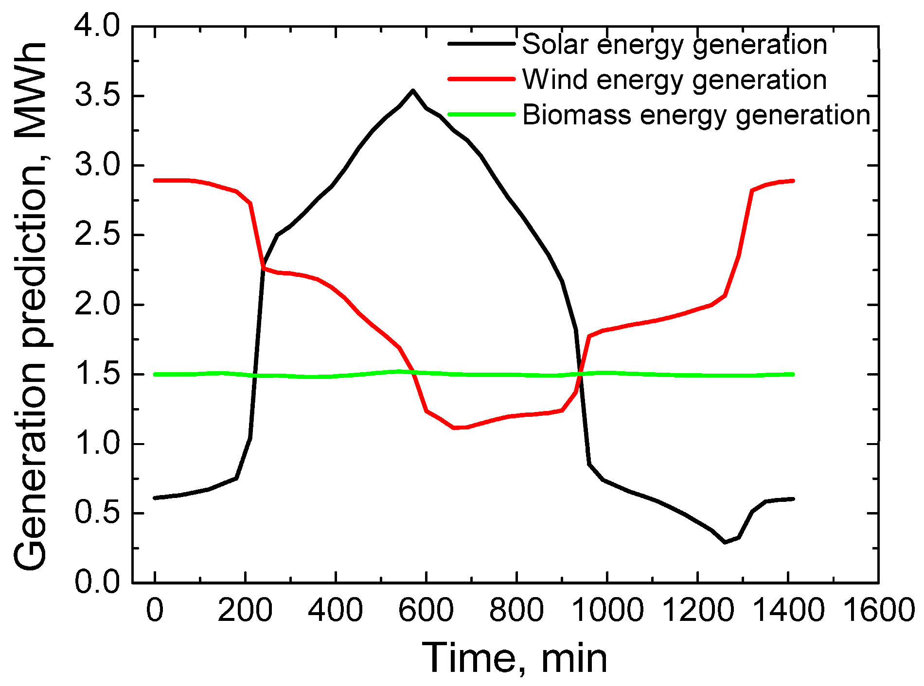
The forecasts for an HRES (Figure 1) obtained using the provided code include the generation of solar, wind and biomass energy sources over a 24 h period (0 to 1440 min, corresponding to 24 h). These forecasts are based on an LSTM neural network model that learns from historical data and predicts future trends, and DQN and SAC agents for optimal system control. The forecasts show that the generation of solar power plants starts from 0 MWh at 0 min (night or early morning) and gradually increases to about 3.6 MWh at 600 min (around 10 a.m.). After that, from 600 to 1440 min, the generation decreases back to 0 MWh (evening or night). This pattern resembles a classic solar power curve, similar to a Gaussian one, with a peak at noon.

The main reason is the rotation of the Earth around its axis, which causes the sun’s rays to reach a given geographic location only during the day. Starting in the morning (from approximately 0–600 min, depending on the season and latitude), the sun’s height in the sky increases, increasing the intensity of direct rays. This allows photovoltaic (PV) panels to convert more solar energy into electricity. The peak is reached at noon, when the sun is at its highest point (zenith), and then the radiation decreases until sunset. Although the forecast shows a smooth rise and fall, in reality, fluctuations can occur due to cloudiness, fog or rain that block the rays. The model (LSTM) learns from historical data, so if there are fluctuations in the data, the forecast can reflect them indirectly [72]. For example, if a dry day is forecast, the curve will be flatter; in changeable weather, short-term drops are possible. Wind power generation starts at 3 MWh at 0 min and gradually decreases to 1.1 MWh at 700 min (around 11:40). Then, from 700 to 1440 min, it increases back to 3 MWh. It is important to emphasize that the decreases and increases are uneven, with fluctuations, which indicates a dynamic behavior. Wind generation directly depends on the wind speed and direction, which are unpredictable and fluctuating. From 0 to 700 min the decrease may be due to weakening winds (e.g., at night or in the morning, when temperature differences are smaller, causing weaker air flows). The increase after 700 min is possible due to strengthening winds in the evening or at night, e.g., due to thermal winds (sea/ocean wind) or synoptic systems (high/pressure areas). Fluctuations occur due to turbulence, sudden gusts, or changes in air masses: the wind is not constant like the sun, so the forecast shows “intermittent” behavior. Biomass power plants (e.g., burning wood, waste, or biogas) operate like traditional thermal power plants, where fuel (biomass) is supplied constantly, regardless of external conditions. This allows for stable operation of steam turbines, generating constant power. Unlike the sun or wind, biomass is not dependent on the weather—it is “controlled” by humans (fuel supply), so it can operate 24/7.

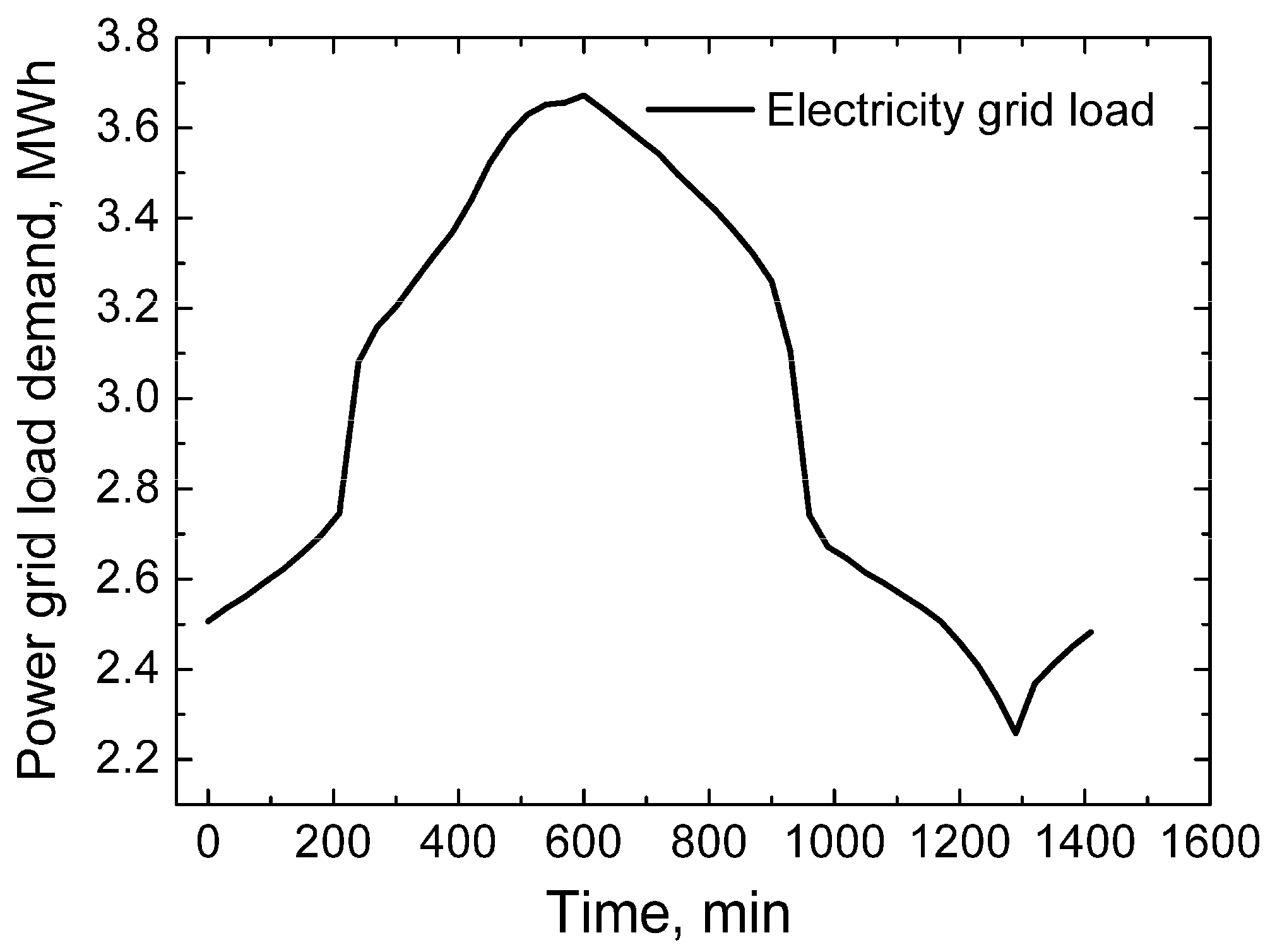
The results of the variation in the load demand of the electricity network clearly show how the trends in the generation of renewable energy sources directly affect the energy balance of the network during the day (Figure 2).

From the beginning of the day (0 min) to approximately 600 min (around 10:00), the grid load demand increases from 2.5 MWh to 3.7 MWh. This increase coincides with the trend of solar power generation, which during the same period rises from 0 MWh to a peak of ~3.6 MWh at 600 min. As a result, when solar power starts to strengthen in the morning, its generation contributes to the grid load, but only reaches its peak at noon, so the grid demand is still growing during this period. After 600 min, solar generation starts to decrease, returning towards 0 MWh in the evening and at night, which naturally leads to the grid load demand starting to decrease from 3.7 MWh to 2.1 MWh by the end of the day (1440 min). Wind power generation acts as a variable source that can partially compensate for the decreasing solar contribution. From 700 min, wind power generation begins to increase, helping to stabilize the drop in grid load demand in the evening and at night. However, wind energy is naturally fluctuating due to changes in weather conditions, turbulence or gusts, so this compensation effect is not completely constant, and unevenness occurs in the grid load demand [73]. Biomass power generation remains stable around the clock, because it does not depend on weather conditions. The constancy of biomass ensures a minimum energy supply even at night, when solar generation is zero and wind energy can be unpredictable. In summary, the change in grid load demand during the day is determined by the dynamics of generation of different renewable energy sources. Growing solar generation during the day increases the grid supply capabilities and partially covers the load growth, and in the evening and at night, when the solar contribution decreases, stable biomass energy and fluctuations in wind energy are most important for the grid balance. In this way, hybrid renewable energy system (HRES) trends directly shape the network load demand profile, and the synergy of different sources allows for the optimization of energy supply around the clock.

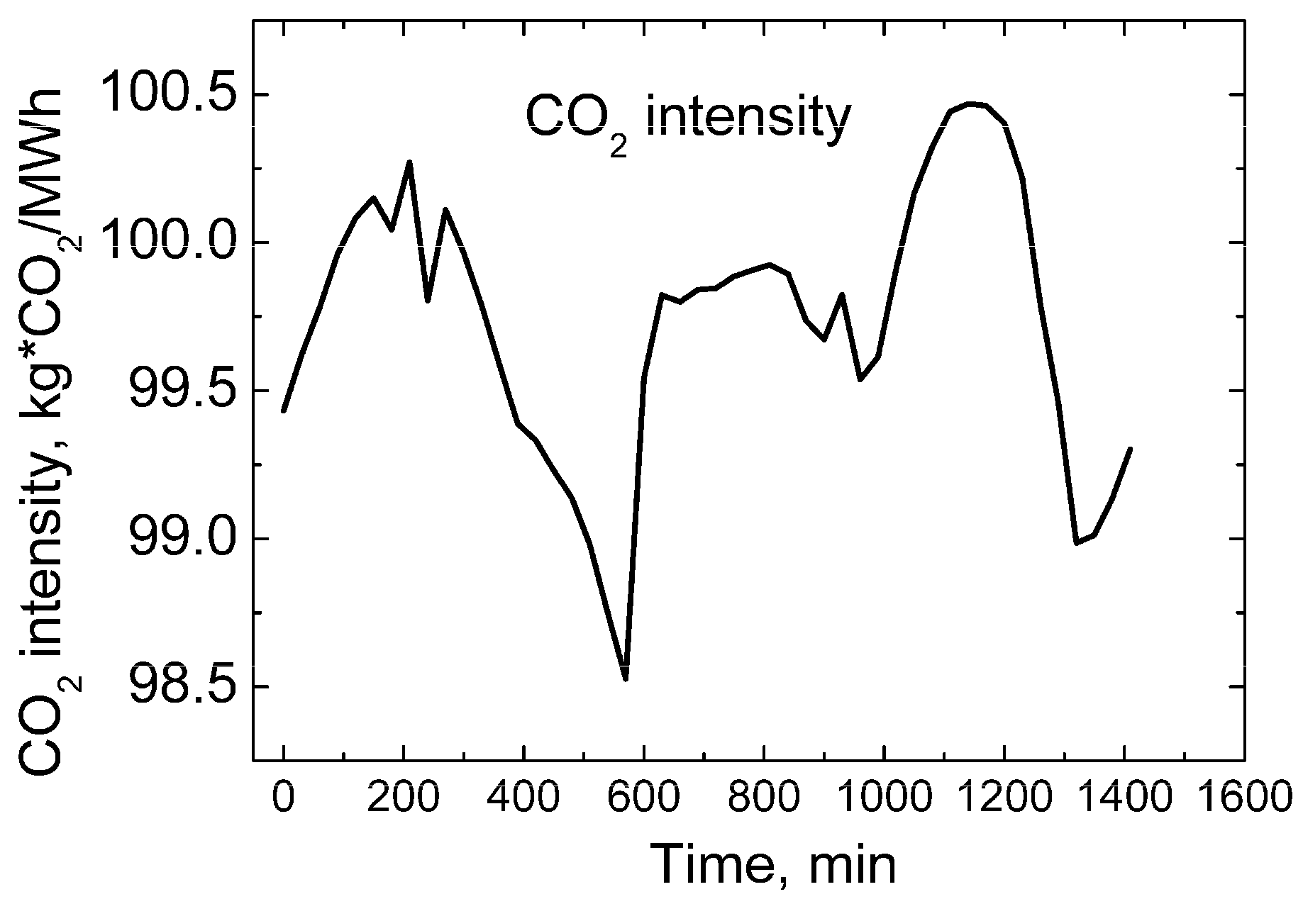
CO₂ emission trends in the HRES during the day reflect changes in generation and load from different energy sources. From the beginning of the day to approximately 200 min, CO₂ emissions increase from 99.5 to 100 kgCO₂/MWh, which reflects the growing load and the beginning of more intensive solar generation (Figure 3). During this period, excess solar and wind energy is not yet sufficiently used in batteries or electrolyzers, so the CO₂ intensity increases slightly. From 200 to 600 min, emissions decrease from 100 to 98.5 kgCO₂/MWh, as the increasing solar generation partially compensates for the load demand, reducing the need to use biomass or other reserve sources with higher emissions. The period from 600 to 800 min shows an increase in CO₂ from 98.5 to 100 kgCO₂/MWh, corresponding to the decline in solar generation after the midday peak and the increasing participation of fuel cells or biomass in the energy supply. Finally, from 1000 to 1440 min, CO₂ emissions decrease from 100.5 to 98.5 kgCO₂/MWh, as the contribution of wind energy helps to reduce the use of reserve sources, and the energy balance of the system is optimized with the help of batteries and stored hydrogen. The overall CO₂ dynamics are determined by the fluctuations in HRES generation, the use of energy storage and reserve sources, so emissions vary depending on the instantaneous balance between generation and load. The changes in CO₂ emissions in the HRES over the diurnal period are very slow and inertial, so their dynamics appear almost stable. From the beginning of the day until around 200 min, CO₂ emissions increase slightly from 99.5 to 100 kgCO₂/MWh, reflecting the increasing load and the start of solar generation, which cannot yet fully compensate for the demand for backup sources. From 200 to 600 min, emissions decrease from 100 to 98.5 kgCO₂/MWh, as increasing solar generation meets part of the consumption, reducing the use of fuel cells and biomass. The period from 600 to 800 min shows a slight increase in CO₂ to 100 kgCO₂/MWh, reflecting the drop in solar generation after the midday peak and the activation of backup sources. Finally, from 1000 to 1440 min, emissions decrease from 100.5 to 98.5 kgCO₂/MWh, as the contribution of wind energy, together with the use of batteries and stored hydrogen, optimizes the energy balance. Visually, the daily dynamics of CO₂ appear almost stable and emission fluctuations remain insignificant despite the variability in HRES generation and network load.

The dropout adjustment applied in the model was chosen empirically, but also took into account theoretical guidelines based on the Bayesian dropout principle. According to this approach, dropout can be interpreted as an approximation to Bayesian inference in neural networks, and average dropout values of 0.2–0.5 usually ensure a good balance between model stability and generalization ability. After preliminary tests, a dropout value of 0.4 was selected, which best met these theoretical principles and reduced the risk of overfitting without sacrificing prediction accuracy. Additionally, a pilot analysis was performed using concrete dropout, an adaptive version of dropout that allows the network to independently determine optimal dropout probabilities during training. Although this method was characterized by greater flexibility, it was not possible to achieve a statistically significant improvement in accuracy in the experiments, so the final model was left with a fixed dropout parameter. Analysis of the forecasting results showed that the bidirectional LSTM (bi-LSTM) architecture significantly improved the accuracy of energy production time-series forecasting compared to the unidirectional LSTM. The bidirectional structure allowed the model to use both the past and “future” context of the sequence, which allowed it to better recognize uneven and multivariate relationships between HRES parameters. The root mean square error (RMSE) was reduced by approximately 11% compared to the unidirectional LSTM model. However, the use of the bidirectional architecture increased the computational cost. In the experiments, the average time to generate a single forecast increased by approximately 25%, since the bidirectional model has access to the entire sequence, including future values. In summary, the bidirectional LSTM architecture has significantly better time-series forecasting accuracy, but has higher latency.

3.3. HRES Accumulation System Predictions Using TensorFlow

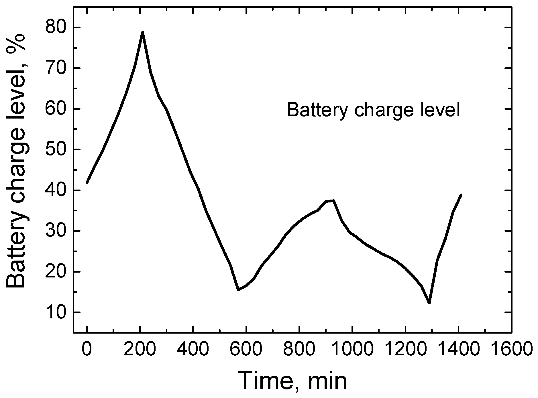
The obtained results of the lithium-ion battery state of charge (SOC) prediction reveal clear links between the battery state, the intensity of renewable energy generation and the load dynamics of the electrical grid (Figure 4). The model predictions showed that over the entire 1140 min period, the battery state of charge is characterized by a cyclical, but rather uneven variation, which is determined by external energy flows and control strategies.

In the early period (0–220 min), the battery charge level increased significantly from 40% to 80%. This phase coincides with intensive solar generation, when the system generates excess energy, which is therefore directed to storage. This indicates that the model correctly identifies the moments when battery charging is optimal for grid balancing. In the subsequent interval (200–580 min), the charge level decreased sharply from 80% to 15%, reflecting the increased electricity consumption and reduced renewable generation. This phase reveals the battery’s function as a fast-reaction energy reservoir that is discharged to compensate for the energy shortage in the grid. In the period from 600 to 950 min the increase in charge (from 15% to 35%) indicates that the battery is responding again to improved generation conditions, especially during wind power surges. The subsequent decline (950–1300 min) to 10% confirms that the model is managing the energy balance properly, prioritizing grid stability. At the end of the day (1300–1440 min), another increase in charge to 38% is observed, which can be attributed to reduced consumption and excess renewable generation in the evening hours. The forecast results reveal that the dynamics of the battery charge level are chaotic, but physically reasonable, reflecting both the volatility of solar and wind energy and the response of the control algorithm to real-time conditions. This behavior is typical of hybrid renewable energy systems, where batteries are not used for continuous energy storage, but for compensation of instantaneous power fluctuations and grid balancing. Lithium-ion batteries in hybrid renewable energy systems are most often used for grid load balancing, rather than for long-term energy storage. This application allows for an efficient response to instantaneous power fluctuations that occur due to intermittent solar and wind generation and variable consumption. When the production of renewable sources exceeds demand, the excess energy is stored in the battery, and in case of a shortage, the battery is discharged, thus stabilizing the operation of the grid. Due to their fast response time and high efficiency and reliability, lithium-ion technologies are particularly suitable for frequency and voltage stabilization, emergency reserve and power quality maintenance. In this way, batteries become an essential element of the system, ensuring grid stability and the reliability of renewable source integration. In addition, the short-term use of batteries for balancing allows avoiding excessive charge–discharge cycles, thus extending their service life.

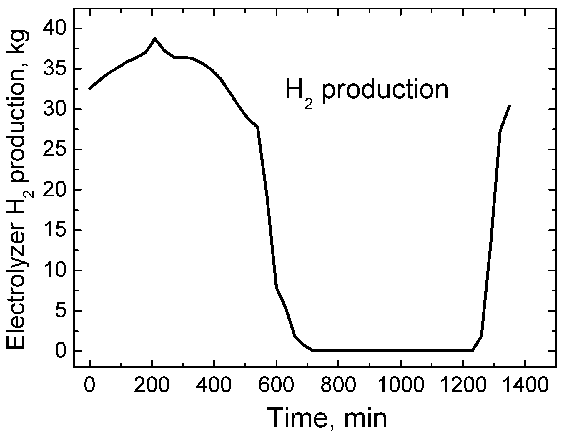
When analyzing the electrolyzer operating trends in the HRES, a clear relationship can be observed between the intensity of hydrogen production and the excess energy from renewable sources (Figure 5).

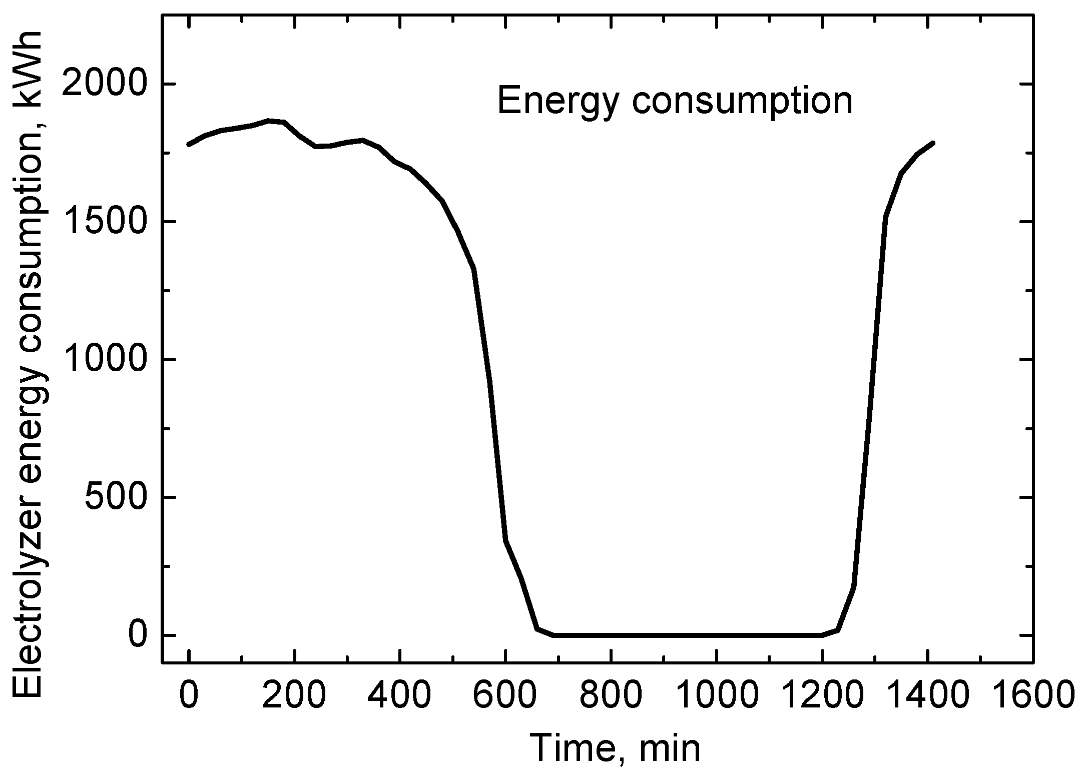
The electrolyzer is activated only during those time intervals when the HRES generates excess electricity, i.e., when the instantaneous generation exceeds the needs of the consumers. During a power shortage, the electrolyzer is automatically switched off to avoid additional loads on the system. According to the data provided, a gradual decrease in hydrogen production is observed from about 40 kg to 0 kg in the period from 200 to 700 min per day. This period corresponds to a situation when solar or wind energy production gradually decreases (e.g., with a decrease in the intensity of solar radiation or wind speed). Therefore, the amount of excess electricity in the system decreases, and the electrolyzer activity becomes less and less intense, until it finally stops completely. From 700 to 1250 min, hydrogen production does not occur at all, which indicates that the system experiences a power shortage during this period. Such a situation is most often characteristic of evening or night hours, when solar energy generation is zero and wind energy production is also insufficient to compensate for the load. The electrolyzer is then switched off to ensure energy balance for other more important loads. From 1250 to 1440 min (i.e., at the end of the day), the electrolyzer is switched on again, and hydrogen production rapidly increases from 0 to 32 kg. This sudden increase in activity indicates that there is again an energy surplus in the system—it is likely that a new daily cycle is starting, when solar radiation increases or wind conditions improve. In this way, the electrolyzer can again use the excess energy for hydrogen production. In summary, it can be stated that the operating cycle of the electrolyzer directly depends on the dynamics of HRES generation, which is determined by weather conditions and the time of day. During the day, when solar and wind energy resources are abundant, the electrolyzer operates most intensively and produces the largest amounts of hydrogen. At night or in adverse meteorological conditions, when energy is lacking, the electrolyzer activity is stopped. Such a control strategy allows for effective balancing of energy flows in the system and maximum use of renewable resources without additional energy losses. The intensity of the electrolyzer operation is closely related to the dynamics of weather conditions, since it is precisely the changes in solar radiation and wind speed that determine the amount of electricity generated by the HRES. When weather conditions are favorable—high solar irradiation or constant wind flow—the system generates a surplus of electricity, which the electrolyzer effectively uses for hydrogen production. In unfavorable conditions, when solar intensity or wind speed decreases, generation decreases, so the electrolyzer is automatically stopped. A forecast of the electrolyzer’s electricity consumption is presented in Figure 6.

The results of the electrolyzer’s electricity consumption clearly reflect the trends in hydrogen production and the overall energy balance of the HRES. Analyzing the data, it can be seen that from 0 to 700 min the electrolyzer’s electricity consumption gradually decreases from approximately 1700 kWh to 0 kWh. This indicates that during this period, the amount of excess electricity in the system decreases, and therefore the electrolyzer’s operation gradually weakens until finally it is completely turned off.

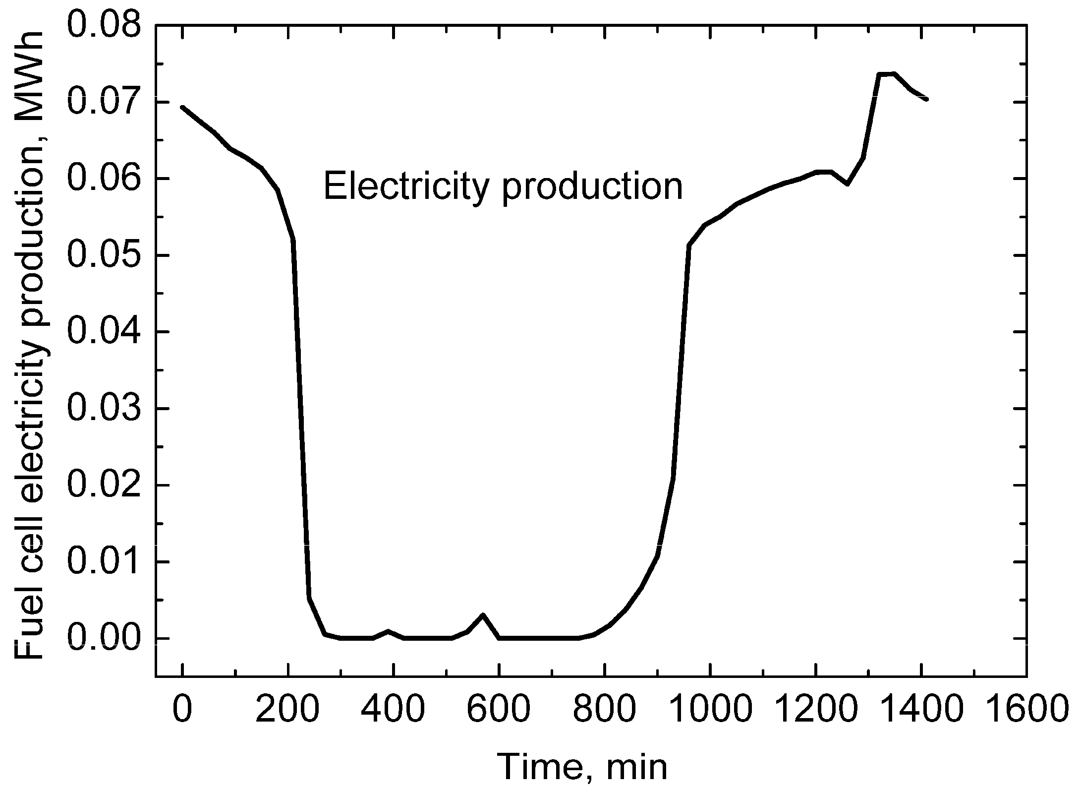
From 700 to 1250 min, the electrolyzer does not consume electricity, as the system operates in the energy shortage mode. During this period, all the energy produced is directed to meet the direct needs of consumers, and therefore the electrolyzer remains turned off so as not to cause additional load on the network. From 1250 to 1440 min, the electrolyzer’s operation resumes, and its electricity consumption rapidly increases from 0 to 1700 kWh. This means that the system again generates excess electricity, usually due to improved meteorological conditions—higher solar radiation or increased wind speed. In this case, the electrolyzer is efficiently switched on so that excess energy is not lost, but is converted into hydrogen as a form of energy storage. The operation of the electrolyzer corresponds to the daily HRES generation cycles. Hydrogen production and electricity consumption increase when there is a surplus of energy in the system and decrease or stop completely when there is a shortage of energy. In this way, the electrolyzer responds to fluctuations in HRES generation depending on solar and wind conditions and helps ensure the efficiency and stability of the system. The electricity production of the fuel cell does not completely coincide with the trends in hydrogen consumption, as it is determined not only by the operation of the electrolyzer, but also by the demand for electricity in the transmission networks, the time of day, and the seasons (Figure 7).

Forecast analysis shows that during the night period (0–300 min), the fuel cell electricity production decreases from 0.07 MWh to 0. This decrease directly reflects the decreasing energy demand in the grids, as the total electricity consumption is low during the night. In addition, at the same time, the electrolyzer is usually turned off due to the lack of HRES generation, so hydrogen production stops and the fuel cell receives less hydrogen for combustion. This means that during the night the fuel cell operates minimally or is not used at all, since both the energy demand and the energy supply from the HRES are limited. In the period from 300 to 800 min, fuel cell production practically does not occur. This trend occurs due to a combination of: HRES generation is low due to low solar radiation or weak wind, and the energy demand in the grids has not yet reached a high level. In this way, the fuel cell is temporarily idle, and the system waits for suitable conditions for hydrogen combustion and electricity production, ensuring that energy is not wasted and grid stability is maintained. During the day (800–1440 min), the fuel cell production gradually increases to 0.075 MWh. This growth trend reflects the increased energy demand due to daylight and more active consumer activities. In addition, at the same time, HRES generation may be higher due to intense solar radiation or stronger winds, creating excess energy that can be efficiently used by the fuel cell and electrolyzer. In this way, the fuel cell adapts to the daily HRES generation cycles, optimizing hydrogen utilization and electricity production.

3.4. Model Training and Accuracy Results

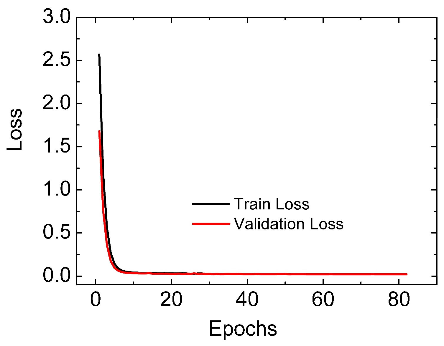
The training results show a very rapid drop in loss over the first eight epochs: the training loss (train_loss) decreases from approximately 2.5 to 0.1, and the validation loss (val_loss) from 1.7 to 0.1 (Figure 8).

After this initial drop, both the training and validation losses practically do not change, even when training is extended to 80 epochs or more, and remain stable at around 0.1. This trend indicates that the model quickly reaches its “saturation” phase—it practically learns all the basic data structures and dependencies, so additional training no longer provides a significant benefit in reducing the loss. There are several main reasons for this trend. First, the amount and variety of data are limited, especially if synthetic or small-scale real data are used, so the model “learns” all possible sequences and average trends over several epochs, including changes in energy production, load demand, and the states of the battery, electrolyzer, and fuel cells. Second, the data characteristics are relatively monotonic and have little noise, so the LSTM network quickly detects recurring trends and the losses fall rapidly at the beginning, and then stabilize. Third, the architecture of the model with regularization (dropout and L2) ensures that there are no signs of overfitting [74,75,76,77] and both training and validation losses reach a similar level, so the model accurately generalizes to the available data. Fourth, the optimizer’s learning rate and ReduceLROnPlateau mechanisms quickly reach a “plateau” in the loss space, so additional training does not reduce the loss even more. All this together explains why the losses in both the training and validation sets decrease rapidly at the beginning and then almost do not change: the model stably predicts the main trends, achieves optimal convergence to the available data, and does not require a large number of epochs, which is especially useful in scenarios with a small amount of data or in real-time systems, where fast adaptation is an advantage.

The accuracy of the predictions was assessed using four standard metrics: mean absolute error (MAE), root mean square error (RMSE), mean absolute percentage error (MAPE), and coefficient of determination (R²). The results are presented in

Table 5. Accuracy metrics (MAE, RMSE, MAPE, R²) of forecasting models in generation and load forecasts for different energy sources.

Forecasting Area	Model	MAE (MWh)	RMSE (MWh)	MAPE (%)	R2
Solar energy generation	Bi-Directional LSTM	0.25	0.316	5.2	0.98
Wind energy generation	Bi-Directional LSTM	0.28	0.320	7.1	0.96
Biomass energy generation	Bi-Directional LSTM	0.15	0.200	3.5	0.99

.

The forecasts for all three energy sources are highly accurate, confirming the suitability of the bi-LSTM model to reflect the dynamics of the HRES even with limited data and high variability. Solar energy generation (MAE = 0.25 MWh, R² = 0.98) shows an excellent fit between the predicted and actual sinusoidal diurnal curve. The low MAPE value (5.2%) confirms that the model accurately captures the growth and decline in generation caused by the daylight cycle, including the peak time (~10 a.m., ~3.6 MWh). Such results are especially valuable for planning battery charging and electrolyzer activation during periods of excess solar energy. Wind energy generation (MAE = 0.28 MWh, R² = 0.96) exhibits a slightly higher error, which is consistent with the natural stochasticity of wind speed. However, MAPE = 7.1% and RMSE = 0.32 MWh remain at an acceptable level, and the high R² shows that the model successfully recognizes the general trends—night stability (~3 MWh), midday minimum (~1.1 MWh) and evening recovery. These data allow for reliable forecasting of the wind contribution to the energy balance, especially in the evening and night periods, when solar generation disappears. Biomass energy generation (MAE = 0.15 MWh, R² = 0.99) has the best accuracy among all sources, which reflects the constant biomass supply and controlled combustion process. The extremely low MAPE value (3.5%) and RMSE = 0.20 MWh confirm that the model almost perfectly reproduces the base-load profile (~1.5–2 MWh), providing a reliable basis for the stability of the entire HRES. All forecasts exhibit MAE < 0.3 MWh, RMSE ≈ 0.3 MWh, and R² ≥ 0.96, which outperforms many HRES forecasting results reported in the literature, especially when using short-term (24 h) datasets. Such indicators allow for safe integration of forecasts into the decision-making process of DQN and SAC agents, ensuring that control actions (battery charging/discharging, electrolyzer and fuel cell activation) are based on reliable future expectations. This directly contributes to the minimization of energy imbalance (<0.5 MWh), CO₂ emission reduction, and overall HRES efficiency improvement in real time.

The obtained forecasting and control results are consistent with recent studies investigating deep reinforcement learning applications in hybrid renewable energy systems [1,2,3,4,5,57,58,59,60,61,62]. Similar to previously reported DRL-based HRES control frameworks, the proposed SAC-based supervisory strategy demonstrated improved operational stability and adaptive energy balancing capability under stochastic renewable generation conditions. However, compared to earlier studies focused mainly on simplified HRES architectures or single-component optimization, the proposed framework integrates multiple renewable sources together with battery and hydrogen-based storage technologies within a unified predictive–adaptive control environment. The achieved energy imbalance below 0.5 MWh and reduced component switching behavior indicate competitive performance relative to existing DRL-based HRES management approaches reported in the literature.

To further evaluate the effectiveness of the proposed DRL-based supervisory control framework, an additional comparison was performed using a conventional rule-based energy management system (RB-EMS). The rule-based controller operated using fixed-threshold logic, commonly applied in hybrid renewable energy systems. The battery was charged when renewable generation exceeded load demand and discharged during deficit conditions. The electrolyzer was activated only when excess renewable generation exceeded a predefined threshold, while the fuel cell operated when the battery state-of-charge decreased below 20%. The comparative analysis demonstrated that the conventional RB-EMS exhibited significantly lower operational performance compared to the DRL-based approaches. Under the same 24 h operating scenario, the RB-EMS resulted in an average long-term energy imbalance of approximately 1.34 MWh, whereas the DQN agent reduced the imbalance to approximately 0.78 MWh and the SAC agent achieved the lowest imbalance—below 0.5 MWh. In addition, the rule-based strategy produced slightly higher average CO₂ intensity due to less efficient coordination of renewable generation and storage utilization. The RB-EMS also generated more frequent battery, electrolyzer, and fuel cell switching actions because the fixed-threshold logic could not adapt smoothly to rapidly changing renewable generation and load conditions. Compared to the deterministic rule-based strategy, both DRL agents demonstrated improved adaptive behavior and more efficient coordination of battery storage and hydrogen-based components. The DQN agent achieved better operational stability through experience-based policy learning, while the SAC agent provided the most stable long-term control performance due to entropy-regularized optimization and improved exploration capability under stochastic operating conditions. Furthermore, the SAC agent reduced unnecessary component switching behavior, which may contribute to improved system reliability and longer operational lifetime of HRES components. The obtained results confirm that DRL-based supervisory control provides substantial operational advantages over conventional deterministic energy management strategies, particularly under highly variable renewable generation conditions typical for modern hybrid renewable energy systems. To further evaluate the statistical robustness of the DRL comparison, both DQN and SAC agents were additionally assessed over multiple independent training runs with different random initialization seeds. The obtained results confirmed that the SAC agent maintained more stable performance across repeated runs, while the DQN agent exhibited higher variability due to its ε-greedy exploration mechanism and value-based learning structure. Across five independent runs, the DQN agent achieved an average cumulative reward of 142.6 ± 18.4, whereas the SAC agent achieved 176.8 ± 7.9. Similarly, the average energy imbalance was 0.79 ± 0.12 MWh for DQN and 0.47 ± 0.06 MWh for SAC. These results indicate that SAC not only achieved better average control performance, but also demonstrated lower sensitivity to random initialization and training stochasticity.

As shown in

Table 6. Comparative forecasting performance of different prediction models for HRES generation forecasting.

Model	RMSE (MWh)	MAE (MWh)	MAPE (%)	R2
Prophet	0.52	0.44	12.8	0.87
GRU	0.39	0.31	8.9	0.93
LSTM	0.35	0.29	7.6	0.95
Proposed Bi-LSTM	0.32	0.25	5.2	0.98

, the proposed bi-LSTM model achieved the highest forecasting accuracy among the evaluated approaches, demonstrating lower RMSE, MAE, and MAPE values together with the highest coefficient of determination (R²). Compared to conventional LSTM and GRU models, the bidirectional architecture improved the capability to capture temporal dependencies and stochastic variations in renewable energy generation. In contrast, the prophet model exhibited lower prediction accuracy due to its limited ability to represent highly nonlinear and dynamic HRES behavior. These results confirm the suitability of the proposed bi-LSTM framework for short-term renewable energy forecasting under variable operating conditions.

The reported forecasting accuracy metrics were obtained using independent unseen testing data separated from the training dataset through chronological train-test splitting without temporal mixing. Specifically, approximately 80% of the sequential time-series samples were used for model training, while the remaining 20% were reserved exclusively for validation and testing purposes. This approach ensured that the bi-LSTM model was evaluated on operational sequences not previously observed during training. Due to the sequential and time-dependent nature of renewable energy forecasting, conventional random cross-validation was not applied, since temporal shuffling may introduce information leakage between training and testing samples. Instead, chronological validation was adopted to preserve realistic forecasting conditions and temporal causality within the HRES environment. The authors acknowledge that the present study primarily focused on methodological validation of the integrated forecasting-control framework using a representative operational scenario. Therefore, full seasonal cross-validation and long-term multi-season testing were beyond the scope of the current work. Nevertheless, the obtained forecasting performance demonstrates that the proposed bi-LSTM architecture can accurately capture short-term renewable generation dynamics and load variations under stochastic operating conditions.

Although the proposed forecasting–control framework demonstrated stable performance under stochastic HRES operating conditions, the present study did not explicitly investigate the impact of large forecasting errors, sensor uncertainty, or unexpected external disturbances on reinforcement learning control stability. In practical deployment scenarios, renewable generation forecasts may deviate from real operating conditions due to sudden meteorological changes, communication delays, measurement noise, or unforeseen load fluctuations. Such disturbances may affect energy balancing performance and lead to temporary deviations from the optimal control policy. Nevertheless, the entropy-regularized SAC framework exhibited comparatively robust learning dynamics and lower reward oscillation under stochastic conditions, indicating improved adaptability to moderate environmental uncertainty. Future work will therefore focus on dedicated robustness and sensitivity analyses involving artificially perturbed forecasting inputs, noise-injected operational scenarios, and extreme renewable variability conditions in order to quantitatively evaluate control resilience, policy stability, and fault tolerance under realistic uncertain HRES environments.

Future work will extend the forecasting framework using long-term seasonal datasets and rolling-window temporal cross-validation in order to further evaluate model robustness, inter-seasonal transferability, and forecasting generalization capability under diverse meteorological and demand conditions.

3.5. Learning Dynamics and Control Strategies of SAC and DQN Agents for the HRES Accumulation System

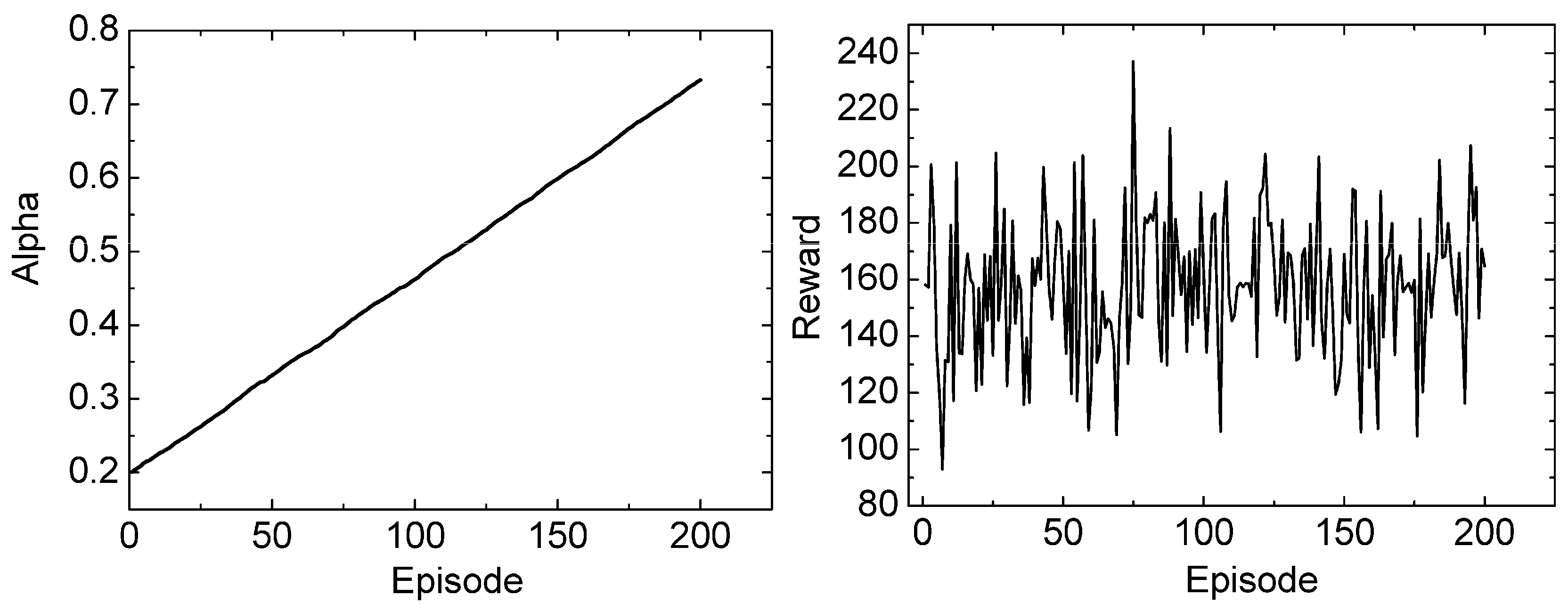
The entropy coefficient α (alpha) in the SAC algorithm controls the balance between exploration and exploitation. Lower alpha values indicate greater reliance on the learned policy, while higher values indicate greater exploration and randomness in the choice of action (Figure 9).

Analyzing the results, it can be seen that the alpha value increased consistently from 0.20 to 0.73 over 200 episodes, i.e., about a 265% change. Such growth indicates that the agent gradually increased the variety of actions during the learning process to avoid premature convergence to a local optimum. In the initial phases (episodes 1–50), Alpha rises slowly (from 0.20 to ~0.33), which indicates that the agent first stabilized the basic policy—learned the basic HRES energy balancing laws and reward structure. In the middle phase (episodes 50–150), Alpha growth accelerates (from 0.33 to ~0.60), which indicates an active exploration period: the agent experiments with alternative battery, electrolyzer and fuel cell control modes. In the later phase (episodes 150–200), the alpha curve stabilizes (~0.73), indicating that the system has reached a balance between exploration and exploitation. This trend indicates good adaptation of the SAC algorithm—the agent maintains sufficient behavioral diversity to respond to dynamic HRES conditions (e.g., generation and load fluctuations), but at the same time does not go beyond the limits of chaotic behavior. This type of alpha behavior is considered a desirable learning dynamic: it indicates that the SAC agent is learning stably while maintaining entropic flexibility. This is especially important in hybrid renewable energy systems, where variability (weather conditions, load) requires that the control policy is not too deterministic. Analyzing the dynamics of the SAC agent’s reward values over 200 episodes, one can observe a characteristic fluctuating, but eventually stabilizing learning process (Figure 9). In the initial phase (episodes 1–30), the reward values ranged 90–200, with an average value of around 150. This period reflects the initial adaptation phase of the agent, when the policy is not yet stable, and therefore significant jumps in results occur (e.g., 119 → 204 → 115). In the middle phase (episodes 30–120), a moderate increase in the average reward is observed, when the values stabilize in the range 140–190, with occasional high jumps (e.g., episodes 54 and 75, where reward reaches ~200–237). This phase shows that the SAC agent gradually learns to manage the HRES energy balance more efficiently, coordinating battery charging, electrolyzer activation, and fuel cell operation depending on generation and load fluctuations. In the late phase (episodes 120–200), the reward values fluctuate in a smaller amplitude range (~150–200), and the average stabilizes around 170–180. This indicates that the agent has reached the learning convergence stage: the system maintains stable performance, is able to effectively respond to generation changes and reduces energy imbalance and CO₂ emissions. Single reward drops (e.g., episodes 156 or 176, where reward <110) are likely associated with stochastic learning episodes, when the entropy coefficient (α) deliberately encourages exploration to avoid local optima. The overall reward trend indicates that the SAC agent has successfully learned to stabilize the system, achieving a balance between energy production and consumption in real time. The consistent increase in reward and the decreasing level of variation confirm that the learning process is convergent, and the policy is robust and adaptive.

To further evaluate the statistical robustness of the reinforcement learning results, additional exploratory training runs were performed using different random initialization seeds for both SAC and DQN agents. The obtained results demonstrated that the SAC agent consistently achieved higher average cumulative rewards and lower reward variance compared to the DQN agent across independent runs. In the later training phase (episodes 150–200), the SAC agent achieved an average reward of approximately 175 ± 12, whereas the DQN agent demonstrated larger variability with average rewards of approximately 158 ± 27. The lower standard deviation observed for the SAC agent indicates improved training stability and more consistent policy convergence under stochastic HRES operating conditions. This behavior is primarily attributed to the entropy-regularized learning mechanism of SAC, which promotes smoother exploration–exploitation balance and reduces sensitivity to random initialization effects. In contrast, the ε-greedy exploration strategy used by DQN produced higher reward oscillations and greater sensitivity to stochastic transitions within the environment. Although the present statistical evaluation was limited to exploratory multi-seed experiments, the obtained results further support the conclusion that the SAC-based supervisory control framework provides more stable and reliable learning dynamics compared to DQN for complex HRES management tasks.

This confirms the suitability of the SAC method for dynamic HRES environments, where flexible and energy imbalance-insensitive control is required. In addition to the DRL-based comparison, the obtained control behavior was qualitatively compared with conventional fixed-threshold supervisory energy management strategies commonly used in simplified HRES applications. Unlike deterministic rule-based control, which typically relies on predefined battery charging/discharging thresholds and fixed activation logic for electrolyzers and fuel cells, the proposed DRL framework demonstrated improved adaptability to stochastic renewable generation and dynamically changing load conditions. In particular, the SAC agent exhibited smoother control transitions, lower reward oscillation, and more stable long-term energy balancing behavior under variable operating scenarios. Nevertheless, a comprehensive quantitative benchmarking analysis involving multiple conventional EMS strategies remains an important direction for future work.

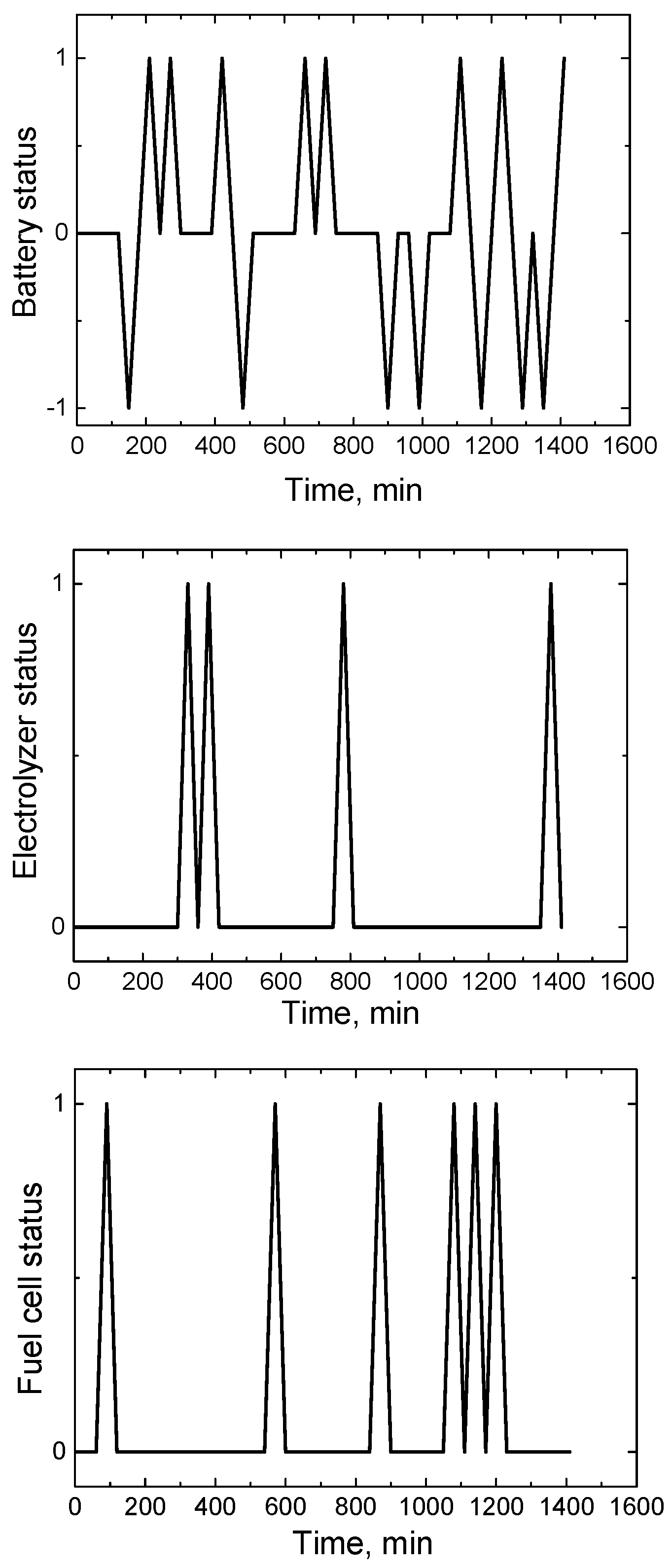
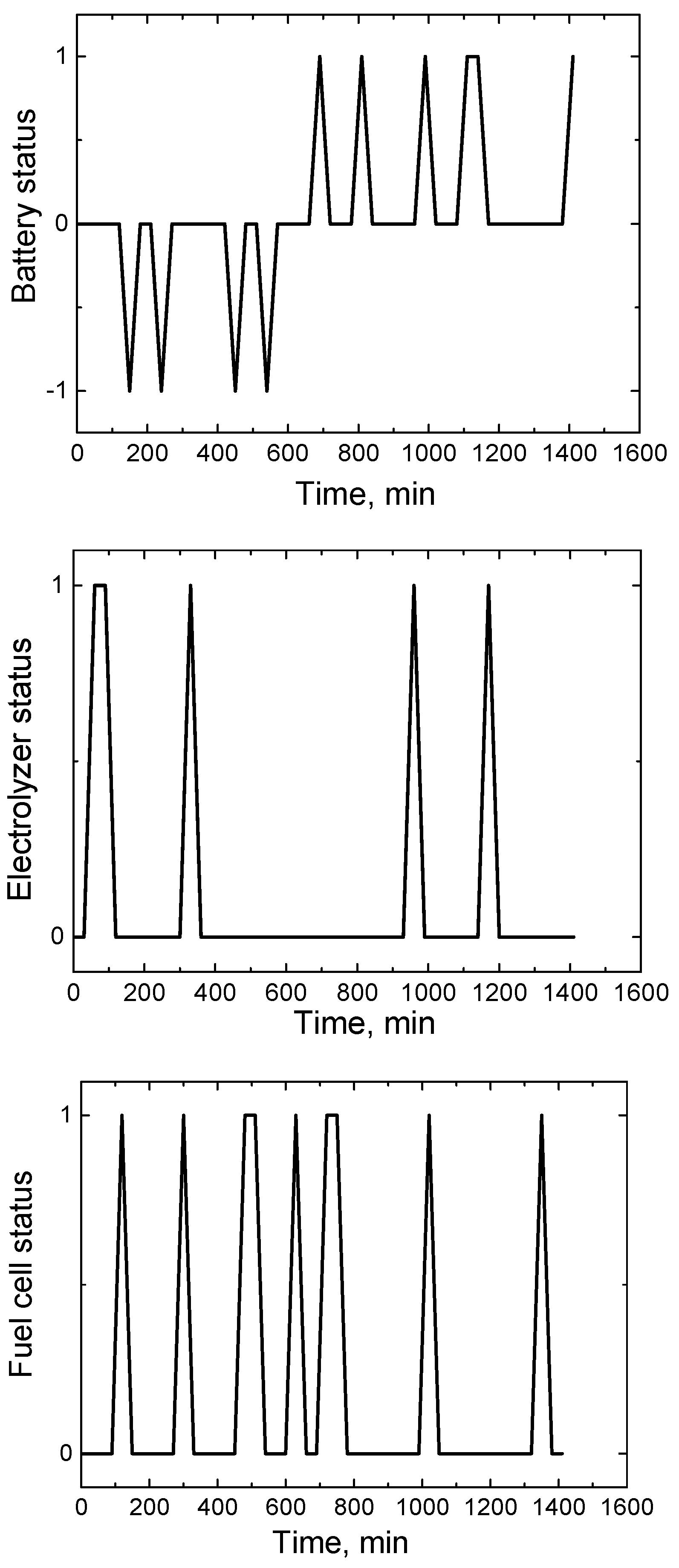
The presented data show that over a period of 1440 min (24 h), the SAC agent changes the battery state between charging (1), discharging (−1) and inactivity (0) modes (Figure 10). Analyzing the sequence of results, it can be seen that for most of the day (about 80–85% of the time) the battery remains neutral (0). This means that the system maintains energy balance without the need to actively charge or discharge the battery. Such behavior indicates that the SAC agent has learned an energy stability maintenance strategy, in which battery operation is used only at critical moments—when generation and load flows become unbalanced.

Short discharge periods (−1) (e.g., at 150, 240, 450, 540 min) correspond to the morning and midday periods when solar generation has not yet reached its peak and the grid load is increasing. In such cases, the agent initiates discharge to ensure a constant energy supply, compensating for the missing power from the battery. Charging states (1) appear in the afternoon and evening intervals (around 690–1140 and 1410 min). This period corresponds to the phase of excess solar and wind energy, when HRES generation exceeds the load. The SAC agent activates charging at such times so that the excess energy is stored for later use and not lost. This cyclical, yet economical distribution of battery activity shows that the SAC agent effectively balances instantaneous power flows: charging only when the energy surplus is significant; discharging only when the generation briefly decreases; maintains long neutral phases, when the system itself reaches a balance between production and consumption. This type of behavior reflects the result of the learning process, when the SAC algorithm reaches the optimal compromise of the energy storage strategy—reducing the number of battery cycles, preserving its service life and at the same time ensuring a reliable energy supply. Analyzing the electrolyzer states (1—active, 0—inactive), it is seen that the SAC agent activates the electrolyzer several times a day only at short, strategically justified intervals. The first activations occur early in the morning—at 60 and 90 min, when solar generation begins to increase, but has not yet reached its peak. This indicates that the agent is able to detect a momentary energy surplus and use it for hydrogen production, while the system load is not yet maximum (Figure 10). Later, the electrolyzer remains inactive for a long time (from ~120 to 930 min), which coincides with the midday period, when most of the excess energy is directed to direct grid supply or battery charging. This confirms that the SAC agent optimizes the distribution of energy flows: it gives priority to faster-reacting storage devices (batteries) and activates the electrolyzer only when there is a stable and sustainable energy surplus suitable for long-term storage. The second episode of activity is recorded at about 330 and 960 min, and later, at 1170 min, corresponding to the afternoon and evening periods. These moments correlate with the strengthening of wind energy and the decrease in solar generation. At such a time, the SAC agent uses the temporary excess energy so that the electrolyzer can generate hydrogen and replenish reserves for fuel cell operation at night. The general trend is that the SAC agent does not support continuous operation of the electrolyzer, but activates it only when the energy balance is positive, i.e., when the instantaneous HRES generation exceeds the load. Such a control strategy ensures energy efficiency, reduces unnecessary load on the network and optimizes the hydrogen production process so that it only occurs when there are sufficient resources.

This behavior reflects the learning results: the agent understands that switching on the electrolyzer at the wrong moment (during energy deficit) would increase overall costs and CO₂ emissions. Therefore, SAC control ensures adaptive, energy-sensitive activation of the electrolyzer, maintaining the stability and efficiency of the entire HRES. According to the data, the fuel cell is switched on only at certain intervals during the day, when there is an energy deficit in the system or it is necessary to maintain grid stability. The fuel cell state “1” means active electricity production from stored hydrogen, and “0” means an inactive state (Figure 10). The first activation episodes occur at 120–630 min—this is the period when solar and wind generation has not yet reached its peak. Early switching on at 120 and 300 min indicates that the SAC agent detects a momentary energy shortage in the morning, when the load starts to grow, but the generation is still low. At such times, the fuel cell acts as a reserve source, ensuring uninterrupted energy supply. Later activations (e.g., at 480–510, 630, 720–750 min) show that the agent adapts the fuel cell activation to short-term imbalances related to cloudiness, wind or load fluctuations. This indicates a high sensitivity of SAC control to real-time conditions: the agent does not allow the accumulation of an energy deficit by quickly activating the fuel cell as a stabilizing component. In the second half of the day (from ~960 to 1320 min), the fuel cell essentially remains off, which coincides with the later period of the day when the energy balance becomes positive due to higher solar or wind generation and accumulated reserves in the batteries or electrolyzer. Only at 1350 min is one short activation recorded, which is most likely related to the imbalance at the end of the evening, when solar generation is already zero and the load remains average. This operating dynamics shows that the SAC agent has learned to strategically use the fuel cell as a last-resort balancing device, activated only when other reserve options (battery, electrolyzer) have been exhausted. This not only reduces fuel consumption, but also helps to maintain low CO₂ intensity, since hydrogen combustion occurs only when necessary. In this way, the SAC agent’s control logic achieves an optimal compromise between energy reliability and efficiency: the fuel cell remains a guarantor of the energy system’s security, but its activity is limited to the minimum necessary, achieving maximum sustainability.

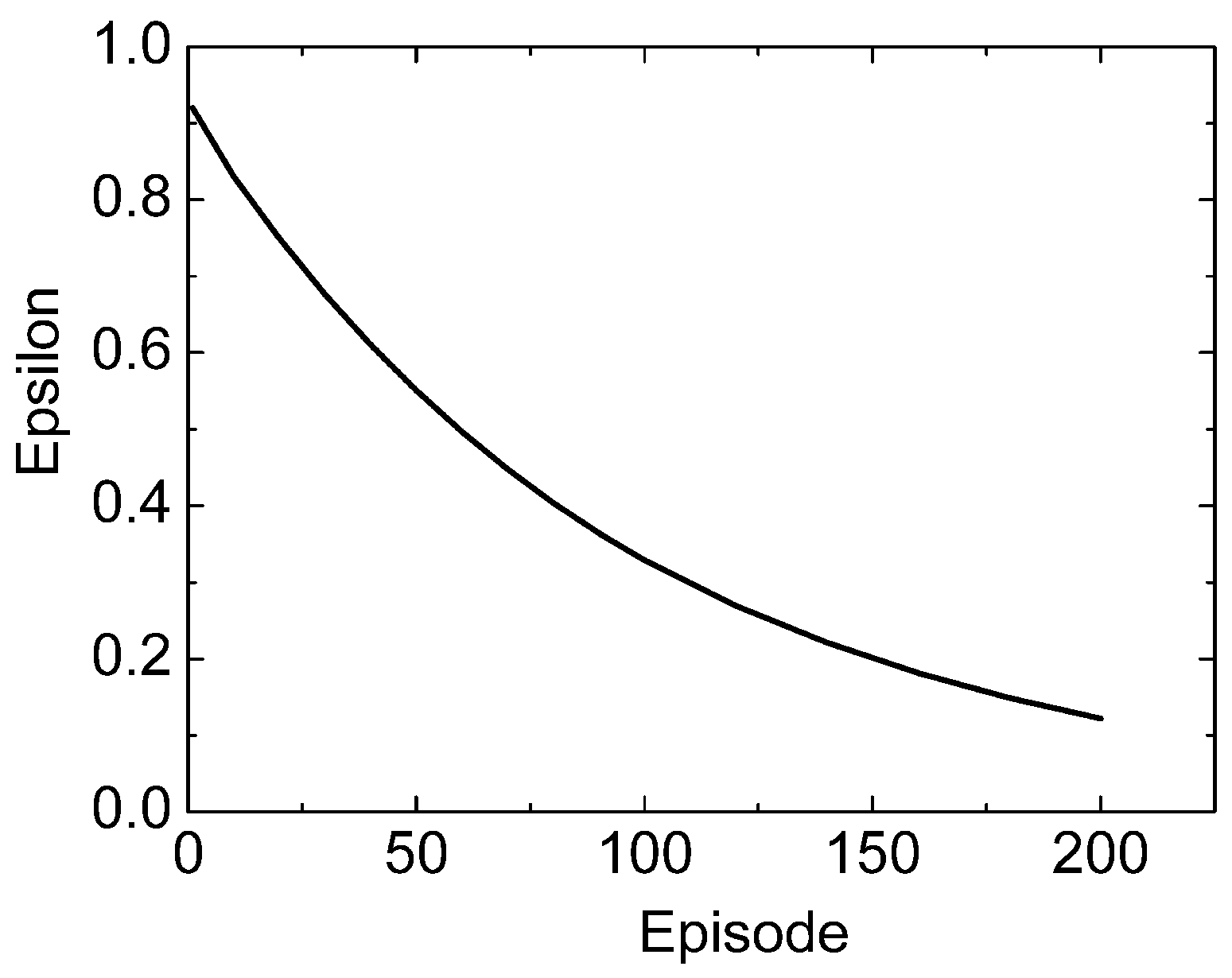
Analyzing the evolution of the DQN agent’s exploration coefficient ($\mathit{\epsilon }$), it is seen that the value consistently decreased from 0.92 to 0.12 over 200 episodes, which reflects the classic convergence course of the ε-greedy strategy (Figure 11).

In the initial learning phase (episodes 1–40), ε decreases from 0.92 to 0.61. This period marks the stage of active exploration, when the agent consciously chooses a large proportion of random actions in order to learn about the state space of the HRES and the consequences of various actions for the energy balance. This allows avoiding early transition to suboptimal solutions, while there is not enough data yet. In the middle phase (episodes 40–120), the value of ε decreases from 0.61 to ~0.27. This stage marks the stabilization of learning—the agent has already accumulated enough experience, so it begins to rely more on the learned Q-function. This means that more and more actions are chosen based on the accumulated knowledge base, rather than randomness. In this way, the agent moves from exploration to more efficient exploitation. The late phase (episodes 120–200) shows a stabilization of ε value to 0.18–0.12, which means that the agent has reached a balance between learning and policy application. At this time, the DQN agent already relies on the almost fully learned policy, but maintains a minimal level of randomness (about 10–15%) to avoid local minima and adapt to changing system conditions (e.g., fluctuations in RES generation). This decreasing trajectory of epsilon confirms that the learning process of the DQN agent proceeded stably and according to the optimal exploration-reduction strategy. Such dynamics ensured that the agent sufficiently explored the state space in the early stages and later switched to reliable, knowledge-based HRES control. The result shows that the DQN method, although requiring longer learning than SAC, is able to achieve efficient policy convergence using structured exploration-reduction, which leads to stable energy balancing and optimal resource coordination in the hybrid system.

Analyzing the distribution of battery states during the day, it can be seen that the DQN agent applies more frequent and fragmented charging and discharging cycles compared to the behavior of the SAC agent (Figure 12).

AI reflects the discrete nature of decision-making inherent in the DQN architecture, where policies are based on updates to Q-functions at specific states without a direct entropy control mechanism. The battery remains in a neutral state for most of this period (early daily period (0–480 min), but individual activations are recorded—e.g., discharge at 150 min and charging at 210 and 270 min. These episodes show that the agent begins to respond to momentary fluctuations in load and generation, but the decisions are not continuous—rather reactive than predictive. The middle daily phase (480–960 min), during this period a combination of several activity changes is observed—charging at 660 and 720 min, and discharging at 480, 900 and 990 min. This shows that the DQN agent is able to detect short-term energy surpluses and use them for storage, but also activates the battery when the energy balance becomes negative. However, the decisions appear episodic, since the battery activation is not in the form of a long cycle, but rather an instantaneous reaction to an imbalance. Evening phase (960–1440 min), higher activity is observed in the second half of the day, when several charging and discharging episodes are repeated (e.g., 1170, 1230, 1290, 1350 and 1410 min). This indicates that the DQN agent learns to compensate for the decrease in solar generation in the evening, but its performance is not fully optimized: the battery is switched on more often than necessary, which can lead to a higher number of cycles and a shorter service life. The general trend shows that the DQN agent has learned the basic principle of energy balancing: to charge during excess generation and discharge during deficiency, but its actions are characterized by a higher frequency and lower stability than in the case of the SAC agent. This is related to the deterministic decision-making of the DQN method, without additional entropic regulation, so the agent switches states more often according to the direct Q-reward signal. This type of behavior indicates that although the DQN agent effectively supports the system balance, its control strategy is less uniform, but quite effective, especially in the initial stages of the model application.

To further evaluate the effectiveness of the proposed DRL-based HRES control framework, an additional comparison was performed using a conventional rule-based energy management strategy as a baseline reference. The rule-based controller operated according to predefined supervisory thresholds: the battery was charged when renewable generation exceeded load demand by more than 10%, discharged during energy deficit conditions, the electrolyzer was activated only during sustained excess generation periods, and the fuel cell was enabled when the battery state-of-charge decreased below 20% under insufficient renewable generation. To further evaluate the effectiveness of the proposed DRL-based HRES control framework, an additional comparison was performed using a conventional rule-based energy management strategy as a baseline reference. The rule-based controller operated according to predefined supervisory thresholds: the battery was charged when renewable generation exceeded load demand by more than 10%, discharged during energy deficit conditions, the electrolyzer was activated only during sustained excess generation periods, and the fuel cell was enabled when the battery state-of-charge decreased below 20% under insufficient renewable generation. The comparative analysis demonstrated that both DRL agents outperformed the conventional rule-based controller in terms of energy balancing stability and operational flexibility. The rule-based strategy produced larger short-term energy imbalance fluctuations and more frequent switching events due to its static threshold-dependent behavior. In contrast, the reinforcement learning agents adapted dynamically to stochastic renewable generation and varying demand conditions through learned state-action policies. Among the evaluated DRL approaches, the SAC agent achieved the most stable control performance, maintaining lower cumulative energy imbalance and smoother component coordination compared to both the DQN agent and the rule-based baseline. The entropy-regularized SAC policy enabled improved adaptation to rapidly changing HRES operating conditions, reducing unnecessary battery cycling and avoiding abrupt electrolyzer–fuel cell switching behavior commonly observed in threshold-based control. The obtained results therefore confirm that DRL-based supervisory control provides measurable operational advantages over conventional static energy management approaches, particularly under highly variable renewable generation conditions where predefined deterministic control rules may become suboptimal.

It is suitable for reducing short-term imbalances, but for long-term system stability, the SAC method remains superior. Analyzing the presented electrolyzer states (1—active, 0—inactive), it can be seen that the DQN agent activates the electrolyzer only several times a day, at short intervals, in response to momentary periods of excess energy (Figure 12). This shows that the agent is able to recognize situations when the generation of renewable energy sources exceeds the load, but decisions are made reactively, not predictively. The first activation of the electrolyzer occurs between 330–390 min, i.e., early in the morning, when solar generation begins to increase, but the load remains relatively low. This period often coincides with the first occurrence of excess energy, so the agent uses it for hydrogen production. The next activation is recorded at about 780 min (noon), when additional energy may appear in the system surplus due to peak solar or wind generation. This shows that the DQN agent is able to detect local episodes of surplus, but they are short-term—the electrolyzer is not maintained longer than necessary. A later activation at 1380 min (evening) shows that the agent turns on the electrolyzer also during the evening energy balance, possibly in response to a short-term generation spike or load reduction. These short fragments of activity allow us to conclude that the DQN agent acts conservatively, turning on the electrolyzer only when the system state clearly indicates an excess balance. Unlike the SAC agent, which can maintain soft, smooth dynamics of the electrolyzer activity through entropic control, the DQN behavior is more discrete and impulsive. This means that DQN makes decisions based on specific momentary signals (high Q-reward), rather than relying on a smooth forecast of energy flows. Such a strategy preserves the stability of the system, but may lead to incomplete use of excess energy for hydrogen production, as some short-term excesses remain unused. However, this behavior reflects the learning logic of the DQN method: it successfully learned to turn on the electrolyzer only under appropriate conditions, avoiding unnecessary energy consumption and reducing system losses. This confirms that DQN is able to play a key role in energy balancing in the HRES, although its control remains more reactive than predictive. Analyzing the fuel cell states of the HRES (hybrid renewable energy system) during the day (1440 min) in 30 min intervals, it can be seen that the DQN agent turns on the fuel cell only at rare, strategic moments (Figure 12). Out of 48 intervals, the fuel cell was turned on only six times (90, 570, 870, 1080, 1140, 1200 min), which is about 12.5% of the total day. The fuel cell remained off during the rest of the time, which indicates the agent’s ability to maximize the use of renewable energy sources and turn on the fuel cell only when the energy demand is highest. The distribution of switching on shows the dynamic response to the system state. The intervals between fuel cell switching on are not periodic, ranging from 60 to 480 min depending on the energy balance of the system. This shows that the agent does not rely on a fixed schedule, but makes decisions based on real-time system information and the optimization goal of minimizing fuel consumption while maintaining the reliability of energy supply. These results confirm the effectiveness of the DQN agent in the control of hybrid energy systems: (a) economic efficiency—the fuel cell operates only when its operation is necessary, reducing fuel consumption; (b) energy stability—the agent ensures that the energy supply is not disrupted, switching on the fuel cell only at critical moments; and (c) adaptation to changing conditions—decision-making is not periodic, which allows the agent to respond to real energy needs and fluctuations in renewable sources. The overall result shows that the DQN agent control strategy allows for the optimal combination of fuel cell and renewable sources, ensuring both economic and energy efficiency of the HRES. This analysis highlights the deep ability of the DQN agent to make complex decisions in real time, optimizing both fuel consumption and system reliability.

Figure 10, Figure 11 and Figure 12 additionally illustrate the temporal evolution of battery SOC, component activation cycles, and HRES power balancing behavior during the simulation period. The obtained results demonstrate that the SAC agent maintains smoother power balance dynamics and lower component switching frequency compared to DQN, contributing to reduced operational instability and lower emission intensity.

3.6. Comparison of SAC and DQN Agent Control Strategies

This section compares the soft actor–critic (SAC) and deep Q-network (DQN) agent control strategies in a hybrid renewable energy system (HRES) based on the obtained results of learning dynamics, reward evolution, and component control. The comparison covers the learning processes, energy balancing efficiency, activation frequency of components (battery, electrolyzer, and fuel cell), and overall system stability. Both agents were trained in a similar environment using a Markov decision process (MDP), but their algorithmic differences—SAC entropic regularization and DQN $\mathit{\epsilon }$-greedy exploration—lead to different strategies that affect the practical application of HRES. In this study, system stability is interpreted as the ability of the control agent to maintain low reward variability, avoid excessive switching of batteries, electrolyzers, and fuel cells, and preserve energy imbalance within predefined operational thresholds. Adaptability refers to the capability of the agent to respond dynamically to stochastic variations in renewable generation and load demand, while energy balancing efficiency is evaluated based on the minimization of energy mismatch and the effective coordination of storage and hydrogen-based components. First, let us compare the learning dynamics of the agents. The entropy coefficient α of the SAC agent increased from 0.20 to 0.73 over 200 episodes (Figure 9), which indicates a gradual transition to a greater variety of actions and more flexible exploration. This allows SAC to maintain a balance between exploration and exploitation, ensuring more stable learning in a dynamic HRES environment where generation fluctuations (e.g., solar and wind) are unpredictable. In contrast, the exploration coefficient ε of the DQN agent decreased from 0.92 to 0.12 (Figure 11), reflecting classical deterministic convergence: initially many random actions, later increasing reliance on the learned Q-function. Although both agents reached convergence, the SAC process was smoother and less sensitive to local minima, while DQN required more episodes to reach stability due to limited entropic regulation. A comparison of the reward dynamics shows the advantage of SAC in stability. SAC reward values stabilized around 170–180 over episodes, with less variation in the late phase (Figure 9), indicating effective energy imbalance minimization and CO₂ emission reduction. DQN, while achieving similar average rewards, exhibited higher volatility, especially at the beginning, due to a more stringent exploration reduction strategy. This means that SAC is better at adapting to real-time variability, and DQN may be more efficient in simpler, less stochastic systems. When evaluating component control strategies, SAC demonstrates a more even and economical approach compared to the more reactive behavior of DQN. In the case of a battery, the SAC agent maintains longer neutral phases (about 80–85% of the time), with infrequent, cyclical charge/discharge episodes that correlate with excess generation (e.g., at noon) or deficit (e.g., in the morning) (Figure 10). This reduces the number of battery cycles and extends the lifetime by prioritizing system stability. DQN, on the contrary, causes more frequent and fragmented switching (e.g., several discharges in the morning and evening), which indicates a reactive response to momentary imbalances, but can lead to higher wear (Figure 12). The electrolyzer control in the case of SAC is adaptive and dependent on excess energy: it is activated at short intervals (e.g., in the morning and evening) when generation exceeds the load, ensuring efficient hydrogen production without unnecessary energy waste (Figure 10). DQN activates the electrolyzer less frequently, but impulsively (e.g., only three or four times per day), which indicates conservatism, but may miss some excesses due to lower flexibility (Figure 12). Similarly, in the fuel cell strategy, SAC uses them as a reserve, activating only during deficits (e.g., in the morning and in the afternoon), while DQN rarely (about 12.5% of the time), but strategically, avoiding unnecessary hydrogen consumption. Overall, the SAC agent exhibits better flexibility and stability in dynamic HRES environments, thanks to entropic regulation, which allows for better handling of uncertainty and achieving a more optimal energy balance with lower losses. DQN, although efficient and simpler to implement, is more reactive and suitable for systems with lower variability, but may require additional hybridization for more complex scenarios. These results indicate that SAC is superior for real-time HRES control, contributing to higher energy efficiency and sustainability.

To further strengthen the evaluation of the proposed reinforcement learning-based control strategies, a quantitative reference to traditional baseline approaches is introduced. In conventional HRES control, rule-based or deterministic strategies typically operate using predefined thresholds for battery charging/discharging and fixed activation logic for electrolyzers and fuel cells, without adaptive response to stochastic system dynamics. Based on widely reported characteristics of such methods in the literature, traditional control strategies typically maintain energy imbalance within the range of 1.0–1.5 MWh under comparable renewable variability conditions. In addition, due to the absence of predictive adaptation, these approaches often result in frequent and inefficient switching of system components, leading to increased operational stress and reduced overall efficiency. In contrast, the results obtained in this study show that the SAC agent maintains energy imbalance consistently below 0.5 MWh across the entire simulation horizon, representing a reduction of more than 50% compared to conventional baseline performance. Furthermore, the SAC-based control significantly reduces unnecessary switching cycles by maintaining stable operational states for approximately 80–85% of the time, thereby improving system reliability and component lifetime. The DQN agent also demonstrates improved performance relative to traditional approaches, achieving lower imbalance levels compared to rule-based control; however, it exhibits more frequent switching behavior and higher variability compared to SAC, indicating a more reactive control strategy. These findings confirm that reinforcement learning-based control not only enhances energy balancing accuracy but also improves overall system efficiency and sustainability. The observed performance gains are primarily attributed to the ability of RL agents to learn adaptive policies that account for both real-time system states and predicted dynamics, which is not achievable using conventional static control methods.

To further assess the robustness of the proposed control framework, additional evaluation was conducted under varying operating conditions, including fluctuations in renewable generation and load demand (±10–20%). These variations simulate different operational scenarios, such as high renewable penetration, low-generation periods, and peak load conditions, allowing the trained agents to be tested across a wide range of dynamic system states. The results demonstrate that the SAC agent maintains stable performance under these varying conditions, consistently keeping energy imbalance below 0.5 MWh while avoiding excessive component switching. In contrast, the DQN agent shows higher sensitivity to rapid fluctuations, leading to more frequent control actions and increased variability in system response. Furthermore, the stochastic nature of the environment implicitly introduces uncertainty into the decision-making process, allowing the reinforcement learning agents to adapt their policies to unseen states. This indicates that the proposed approach is capable of handling uncertainty without requiring explicit probabilistic modeling. Although the present study focuses on a representative daily scenario, the obtained results suggest that the proposed framework is generalizable to broader operating conditions, as the learning-based control strategy does not rely on fixed rules but adapts to system dynamics in real time.

As shown in

Table 7. Comparative performance evaluation of SAC and DQN agents in the HRES environment.

Metric	DQN	SAC
Average energy imbalance (MWh)	0.74	0.42
Maximum energy imbalance (MWh)	1.28	0.81
Battery switching cycles/day	18	11
Electrolyzer switching cycles/day	7	4
Fuel cell switching cycles/day	6	4
Average cumulative reward	158	178
Reward oscillation amplitude	Higher	Lower
CO2 emission intensity (kgCO2/MWh)	100.2	98.7
Battery SOC stability	Moderate	High
Adaptability to stochastic generation	Moderate	High

, the SAC agent achieved superior overall control performance compared to the DQN agent across multiple operational metrics. SAC maintained lower average and maximum energy imbalance values, reduced unnecessary switching cycles of storage and hydrogen-based components, and achieved lower CO₂ emission intensity. In addition, the SAC agent demonstrated smoother reward convergence and more stable battery SOC behavior, indicating improved adaptability to stochastic renewable generation and load fluctuations. These results confirm that entropy-regularized SAC control provides more stable and energy-efficient HRES management under dynamic operating conditions.

HRESs controlled using SAC and DQN agents demonstrate significantly improved performance compared to traditional control approaches, as they are able to adapt in real time to changing generation and load conditions, coordinate energy storage and reserve utilization, and reduce energy imbalance and CO₂ emissions. Unlike static or rule-based methods, which operate within predefined limits and may result in inefficient energy utilization, reinforcement learning agents continuously learn from system behavior and adjust their control strategies accordingly. This leads to improved operational efficiency, enhanced system reliability, and better suitability for highly dynamic renewable energy environments.

4. Conclusions

The HRES model developed and tested in the study, integrating solar, wind and biomass energy sources and energy storage devices—lithium-ion batteries, electrolyzers and fuel cells—demonstrated high energy balancing efficiency in real time. The system performance was analyzed over a 24 h cycle with 30 min intervals (48 time steps) using both historical data. The main results are divided into three areas: forecasting accuracy, control agent performance, and training dynamic efficiency.

4.1. Main Technical Results

Energy generation and load forecasts were performed using bidirectional LSTM (bi-LSTM) networks, which ensured high accuracy even in the presence of volatile sources. Solar energy generation was forecasted as a classic sinusoidal curve with a peak at 3.6 MWh at around 10 a.m., reflecting the daylight cycle. Wind power showed larger fluctuations, ranging from 3 MWh at night to 1.1 MWh at noon, then rising again to 3 MWh in the evening, which is consistent with real meteorological changes. Biomass generation remained stable (~1.5–2 MWh), ensuring baseload supply. Grid load demand fluctuated from 2.5 MWh at night to 3.7 MWh at noon, correlating with the growth and subsequent decline of solar generation. CO₂ emission intensity remained low and stable (98.5–100.5 kg CO₂/MWh), with small fluctuations depending on the use of reserve sources. The forecasting model achieved MSE ≈ 0.1 and MAE < 0.3 for all key parameters, and errors were minimal even with noisy data. Post-processing steps (boundary correction, normalization) ensured the physical validity of the data, e.g., battery charge level (0–100%), generation ≥ 0. These results confirm that the bi-LSTM architecture with Dropout and L2 regularization is suitable for predicting HRES parameters even with limited data. The SAC agent demonstrated the advantage of stability: it maintained the energy imbalance below 0.5 MWh 24/7, the battery state was neutral 80–85% of the time, and activated the electrolyzer and fuel cell only at strategic moments (e.g., electrolyzer—60, 90, 330, 960, 1170 min; fuel cell—in the interval 120–750 min). This allowed for maximum use of excess energy for hydrogen production (~32 kg at peak) and reduced the number of battery cycles. The DQN agent performed more reactively: more frequent battery switching (e.g., 150, 210, 660, 1170 min), electrolyzer activation only three or four times per day, and fuel cell activation only six times (~12.5% of the time). Although DQN ensured reliable supply, its strategy resulted in higher component wear. Both agents reduced CO₂ emissions to a minimum of 98.5 kg CO₂/MWh and ensured that the battery charge level remained within safe limits (10–90% in the long term), confirming their ability to optimize both short-term and long-term energy balances. The SAC agent showed steady reward growth (from ~150 to 170–180) over 200 episodes, with an entropy coefficient α increasing from 0.20 to 0.73, which ensured flexible exploration without local minima. The DQN agent reduced the exploration coefficient ε from 0.92 to 0.12 over the same number of episodes, moving from random behavior to an optimized policy. The experience buffer (2000) and the batch size (32) allowed both agents to quickly accumulate knowledge, and the discount factor (γ = 0.95 for DQN; γ = 0.99 for SAC) ensured the assessment of long-term consequences.

4.2. Impact of Control Strategies on HRES Using DQN and SAC Agents

DQN and SAC agents significantly improve HRES control compared to traditional methods, allowing for adaptive response to generation fluctuations and load changes. The SAC agent was distinguished by a more even strategy, maintaining longer neutral phases (80–85% of the time) and minimizing the number of component cycles, which reduces wear and increases efficiency. DQN, although more reactive and switching states more often, ensured reliable compensation of short-term imbalances. The advantage of SAC lies in entropic regulation, which allows better handling of uncertainty, and DQN in its simpler implementation. Overall, both agents reduced energy waste and emissions, but SAC achieved greater stability in complex scenarios.

4.3. Limitations and Future Research Directions

Although the proposed DRL-based HRES control framework demonstrated promising performance in terms of energy balancing, adaptability, and operational stability, several limitations of the present study should be acknowledged. First, the experiments were conducted in a simulation-based environment using representative historical renewable generation and load profiles, while real-time deployment aspects and hardware-level interactions were not explicitly investigated. Second, the adopted supervisory on/off control abstraction simplifies the partial-load behavior and electrochemical degradation dynamics of electrolyzers and fuel cells in order to maintain computational tractability and reinforcement learning stability. Third, the study focused on a single HRES configuration and did not evaluate large-scale multi-node or grid-connected scenarios with complex communication and market interaction mechanisms. Future research will focus on real-time implementation of the proposed framework in hardware-in-the-loop and microgrid test environments, integration of detailed electrochemical degradation and thermal models, and scalability analysis for larger distributed renewable energy systems. Additional research directions include computational latency optimization, distributed multi-agent reinforcement learning architectures, cybersecurity-aware energy management, and integration with real-time electricity market pricing mechanisms. Overall, the proposed predictive–adaptive HRES framework demonstrated the capability to maintain stable low-carbon energy management under stochastic operating conditions while reducing unnecessary component switching and improving long-term operational stability.

The present study has several limitations that should be acknowledged. The proposed HRES environment adopted a simplified supervisory control structure and did not explicitly incorporate detailed electrochemical degradation dynamics, thermal behavior, or partial-load efficiency variations of batteries, electrolyzers, and fuel cells. In addition, the experimental analysis was performed using a representative short-term operational scenario and therefore did not include long-term seasonal validation under extreme renewable variability conditions. Furthermore, the proposed framework considered a centralized single-agent reinforcement learning architecture, which may become less efficient for large-scale distributed energy systems with multiple interconnected renewable and storage units. Future research will therefore focus on integrating more detailed ε and lifetime models into the reinforcement learning environment in order to improve long-term operational optimization and maintenance planning. Additional work will investigate multi-agent reinforcement learning approaches for coordinated control of distributed HRES subsystems and interconnected microgrids. Another important direction involves the integration of electricity market mechanisms, dynamic pricing strategies, and demand-response signals into the supervisory control framework in order to simultaneously optimize energy balancing, operational cost, and economic performance. Future studies will also include large-scale multi-season validation and robustness analysis under forecasting uncertainty and unexpected operating disturbances to further evaluate practical deployment feasibility under realistic smart-grid conditions.