An Urbanization-Aware Remote Sensing Ecological Index for Urban Ecological Quality Assessment: A Case Study of Hangzhou, China

Abstract

Rapid urban expansion has intensified interactions between human disturbance and urban ecological processes, creating an urgent need for robust and urban-sensitive assessment tools. To improve the applicability of conventional remote sensing ecological evaluation in cities, this study develops an Urban Remote Sensing Ecological Index (URSEI) by incorporating an Urbanization Index (UI) into the RSEI-based PCA framework. Multi-temporal Landsat observations acquired during the peak vegetation season were used to construct annual ecological indicators, thereby improving the temporal representativeness of ecological assessment. Taking Hangzhou, China, as a case study, URSEI was applied to examine ecological quality dynamics inside and outside the Ecological Conservation Redline (ECR) from 2010 to 2024, together with temporal trend characteristics, indicative persistence patterns, and meteorological associations. The results show that URSEI generally achieved higher first principal component contribution rates than RSEI, suggesting stronger integration of ecological information within the PCA framework. UI exhibited the strongest negative correlation with URSEI among the stress-related indicators, highlighting the importance of explicitly representing urbanization-related disturbance in urban ecological assessment. Citywide ecological quality displayed a fluctuating but weakly improving tendency over the study period, while the ECR consistently maintained higher URSEI values than the overall urban area. However, most detected temporal changes were statistically non-significant, indicating that ecological conditions remained broadly stable rather than showing pronounced improvement or degradation. Temperature-related thermal conditions were predominantly negatively associated with URSEI, whereas precipitation showed mainly positive relationships and a stronger association with URSEI among the climatic variables examined. Overall, URSEI provides an urbanization-aware framework for long-term ecological monitoring and offers a useful basis for ecological management and sustainable planning in rapidly urbanizing regions.

1. Introduction

Urbanization is a major driver of socio-economic development and simultaneously reshapes land-use patterns and urban ecosystem dynamics [1,2]. In China, where the urbanization rate has approached 70%, the accelerated expansion of cities has introduced multiple sustainability challenges, including hydrological imbalances, urban heat islands, and degradation of ecological conditions [3]. Cities, as the main carriers of human activity and economic production, require systematic and continuous monitoring of ecological quality to inform sustainable planning and governance. Understanding the spatial and temporal dynamics of urban ecological conditions and their driving factors is therefore essential for evidence-based urban management.

The intensification of urban development generates complex spatial heterogeneity in ecological pressures. Different functional land-use types—such as industrial zones, high-density residential areas, low-rise built-up districts, and green or undeveloped spaces—exert varying ecological impacts, highlighting the necessity of frameworks capable of distinguishing these functional differences to accurately assess urban ecological quality.

Advances in remote sensing have enabled efficient, large-scale, and temporally explicit monitoring of urban ecosystems [4]. Traditional single-indicator approaches, including NDVI [5,6], land surface temperature, and built-up indices, primarily capture individual environmental dimensions but often fail to reflect the integrated, multidimensional nature of urban ecological systems [7,8,9,10]. Comprehensive indices, such as the Ecological Environment Index (EI) and the Remote Sensing Ecological Index (RSEI), provide more holistic assessments. Nevertheless, EI often depends on manually assigned weights and heterogeneous data sources, which may introduce subjectivity and reduce reproducibility [11]. Moreover, most conventional approaches rely on single-date imagery, which can introduce phenological bias and reduce temporal representativeness, limiting the robustness of annual ecological evaluations.

To overcome these limitations, we developed the Urban Remote Sensing Ecological Index (URSEI), which extends the conventional RSEI by incorporating the Urbanization Index (UI) directly into PCA [12,13,14]. This integration allows anthropogenic disturbance to be reflected within the composite index, providing a more comprehensive representation of human pressures. Compared with prior RSEI variants, URSEI explicitly integrates urbanization intensity, enhancing the ability to assess urban ecological quality by considering both natural and human-induced factors in complex urban environments [15]. By doing so, URSEI captures the interactive effects between urban development and ecological components, improving the interpretability and robustness of urban ecological assessments [16].

By employing multi-temporal Landsat observations during the peak vegetation season (June–September), URSEI improves the temporal representativeness of annual ecological assessment. Meanwhile, the incorporation of urbanization intensity provides a basis for interpreting ecological differences among areas with contrasting development characteristics, such as densely built-up regions and vegetation-dominated spaces [17,18]. This framework enhances the representation of interactions between natural environmental conditions and anthropogenic pressures in urban ecological assessment.

Using Hangzhou as a case study, we applied URSEI to monitor ecological quality dynamics from 2010 to 2024 within and outside the Ecological Conservation Redline (ECR), and to investigate dominant climatic drivers of variation. The results demonstrate that URSEI provides a novel, urbanization-aware framework for long-term monitoring of urban ecological quality, supports evidence-based urban environmental management, and informs sustainable planning decisions in rapidly urbanizing regions.

2. Study Area and Data

2.1. Study Area

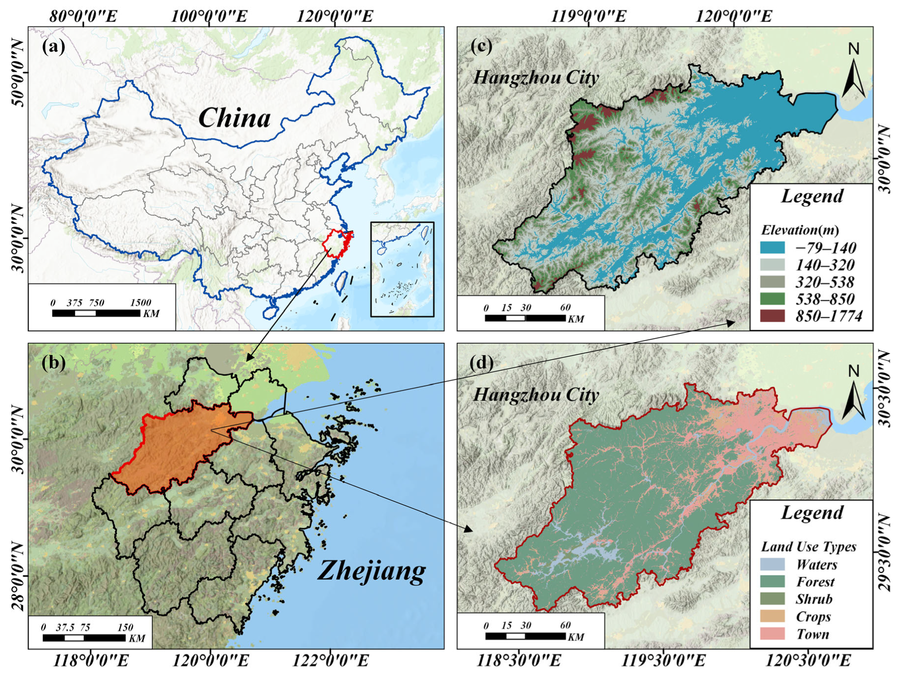
Hangzhou, located in northern Zhejiang Province, spans latitudes 29°11′–30°34′ N and longitudes 118°20′–120°37′ E. As a central city in the Yangtze River Delta, it encompasses approximately 16,850 km² [19] and hosts a permanent resident population of 12.624 million. The city experiences a subtropical monsoon climate, characterized by short spring and autumn seasons, and longer winter and summer periods, with an average annual temperature of 19 °C and total annual precipitation of 1655 mm (Figure 1).

Topographically, the western, central, and southern regions are mainly hills and mountains, covering 65.6% of the total area [20], while the northeastern plains account for 26.4%. Forests cover 65.74% of the city, the highest among provincial capitals in China. The complex terrain and varied land cover patterns influence urban ecological processes, providing a representative setting to study the impacts of urbanization on ecosystem dynamics.

2.2. Data and Preprocessing

(1)

Remote sensing data.

Based on the GEE platform, Landsat 5 and 8 multispectral data at Level 2 were selected as the primary data source for calculating each ecological component. Data was collected for even-numbered years from 2010 to 2024. Because suitable 2012 imagery satisfying the data availability and quality requirements was insufficient for constructing a spatially complete annual ecological dataset, the corresponding temporal node was represented using 2011 observations. To avoid overinterpreting this substitution, the subsequent temporal analysis focuses primarily on broader multi-year ecological variation patterns rather than on isolated year-to-year changes around this substituted time point. Data for each year were selected from June to September, the period of peak vegetation growth, to represent the region’s optimal ecological quality throughout the year. To mitigate the impact of interannual temporal variations within the time series on experimental results, the average values for the five ecological components in the study area were calculated for the June–September period. Specifically, Landsat Collection 2 Level-2 surface reflectance and surface temperature products were used for ecological indicator calculation. Cloud- and cloud-shadow-contaminated pixels were excluded using the QA_PIXEL quality assessment band. The optical surface reflectance bands were converted using the scale factor of 0.0000275 and an additive offset of −0.2, while the surface temperature band was scaled using a factor of 0.00341802 and an additive offset of 149.0. After quality masking and radiometric scaling, all valid observations acquired from June to September in each selected year were aggregated using the arithmetic mean to generate annual ecological indicator layers. All Landsat-derived ecological indicators were generated at a 30 m spatial resolution and spatially aligned to a common analysis grid before subsequent PCA-based index construction.

(2)

Meteorological data.

Obtain the annual total precipitation within the study period from the TerraClimate dataset using the GEE platform. TerraClimate data has a spatial resolution of approximately 4 km, covering multiple climate elements from 1958 to the present. In the study, monthly precipitation data for all 12 months of the year were summed to obtain annual total precipitation. The data were then resampled to a 30 m resolution using bilinear interpolation to ensure spatial consistency across different data sources. The MODIS MOD11A2 LST data released by NASA was obtained via the GEE platform as a thermal environment indicator variable. This product provides 8-day composite daytime land surface temperature data with a spatial resolution of 1 km. This study calculated the annual average land surface temperature for the study area during the research period, also employing bilinear interpolation to resample the resolution to 30 m.

3. Study Methods

3.1. Construction of the Ecological Index

The Remote Sensing Ecological Index (RSEI) provides a comprehensive characterization of regional ecological quality by integrating multiple ecological dimensions and capturing both temporal variability and spatial heterogeneity in ecological conditions. The construction of RSEI involves four ecological indicators, namely greenness ($G$), wetness ($W$), thermal intensity ($T$), and dryness ($D$) [12]. The mathematical expression is as follows:

$$RSEI=f\left(G,W,T,D\right)$$

(1)

The UI proxy was selected because it can be directly derived from the same Landsat observations used for the other ecological components, ensuring spatial resolution consistency, temporal comparability, and methodological reproducibility across the 2010–2024 study period. Compared with alternative urbanization measures such as night-time light intensity, population density, land-use statistics, or external impervious surface products, the selected UI provides a pixel-level spectral representation of built-up intensity without introducing additional cross-source inconsistencies. Moreover, unlike NDBSI, which mainly reflects surface dryness and bare-soil exposure, UI is specifically used here to characterize urbanization-related surface transformation and anthropogenic disturbance. Therefore, UI is suitable for incorporation into the PCA-based ecological index as an internal urbanization pressure component.

Given that urbanization is a major anthropogenic factor influencing ecological quality in urban environments, this study extends the conventional RSEI framework by introducing an urbanization indicator to explicitly represent ecological disturbance associated with urban development. Accordingly, an Urban Remote Sensing Ecological Index (URSEI) is constructed by incorporating the Urbanization Index (UI) into the original RSEI framework, thereby enabling a more complete assessment of ecological quality dynamics under urbanization pressure. By embedding UI within the composite index rather than treating it as an external explanatory variable, URSEI can directly represent urbanization-related ecological pressure and enhance sensitivity to spatial heterogeneity associated with varying levels of urban development. The mathematical expression of URSEI is as follows:

$$URSEI=f\left(G,W,U,T,D\right)$$

(2)

In the proposed framework, greenness is measured by the Normalized Difference Vegetation Index (NDVI), which indicates vegetation growth conditions and surface vegetation cover [21]. Wetness is represented by the wetness component (WET) derived from the Tasseled Cap transformation and is used to describe surface moisture conditions [22]. Urbanization intensity is expressed by the Urbanization Index (UI), which characterizes the degree of urban development and anthropogenic disturbance [23]. Thermal intensity is represented by Land Surface Temperature (LST), which reflects the thermal conditions of the urban surface [24]. Dryness is measured using the Normalized Difference Bare Soil Index (NDBSI), derived from the Bare Soil Index (SI) and the Index-Based Built-up Index (IBI) [25], and is used to characterize surface dryness and bare-soil exposure in urban areas [26]. The mathematical expressions of all ecological components are listed in

Table 1. Mathematical expressions of ecological components.

Index	Formula
NDVI	$NDVI={\displaystyle \frac{{\rho }_{nir}-{\rho }_{red}}{{\rho }_{nir}+{\rho }_{red}}}$
WET	${WET}_{TM}=0.0315{\rho }_{blue}+0.2021{\rho }_{green}+0.3102{\rho }_{red}+0.1594{\rho }_{nir}-0.6806{\rho }_{swir1}-0.6109{\rho }_{swir2}$
	${WET}_{OLI}=0.1511{\rho }_{blue}+0.1973{\rho }_{green}+0.3283{\rho }_{red}+0.3407{\rho }_{nir}-0.7117{\rho }_{swir1}-0.4559{\rho }_{swir2}$
UI	$UI={\displaystyle \frac{\left({\rho }_{swir2}{-\rho }_{nir}\right)}{\left({\rho }_{swir2}{+\rho }_{nir}\right)}}$
LST	$T={\displaystyle \frac{K_2}{\ln \left(\frac{K_1}{L}+1\right)}}$
	$LST={\displaystyle \frac{T}{\left[1+\left(\frac{\lambda T}{\rho }\right)·\ln \epsilon \right]}}-273$
NDBSI	$SI={\displaystyle \frac{\left({\rho }_{swir1}+{\rho }_{red}\right)-\left({\rho }_{nir}+{\rho }_{blue}\right)}{\left({\rho }_{swir1}+{\rho }_{red}\right)+\left({\rho }_{nir}+{\rho }_{blue}\right)}}$
	$IBI={\displaystyle \frac{\left\{\frac{2{\mathsf{\rho }}_{swir1}}{\left({\mathsf{\rho }}_{swir1}+{\mathsf{\rho }}_{nir}\right)}-\left[\frac{{\mathsf{\rho }}_{nir}}{\left({\mathsf{\rho }}_{nir}+{\mathsf{\rho }}_{red}\right)}+\frac{{\mathsf{\rho }}_{green}}{\left({\mathsf{\rho }}_{green}+{\mathsf{\rho }}_{swir1}\right)}\right]\right\}}{\left\{\frac{2{\mathsf{\rho }}_{swir1}}{\left({\mathsf{\rho }}_{swir1}+{\mathsf{\rho }}_{nir}\right)}+\left[\frac{{\mathsf{\rho }}_{nir}}{\left({\mathsf{\rho }}_{nir}+{\mathsf{\rho }}_{red}\right)}+\frac{{\mathsf{\rho }}_{green}}{\left({\mathsf{\rho }}_{green}+{\mathsf{\rho }}_{swir1}\right)}\right]\right\}}}$
	$NDBSI={\displaystyle \frac{SI+IBI}{2}}$

Notes: NDVI, Normalized Difference Vegetation Index; WET, wetness; LST, Land Surface Temperature; SI, Bare Soil Index; IBI, Index of Building Intensity; NDBSI, Normalized Difference Bare Soil Index. ${\rho }_{blue}$, ${\rho }_{green}$, ${\rho }_{red}$, ${\rho }_{nir}$, ${\rho }_{swir1} and {\rho }_{swir2 }$ correspond to the reflectance of the blue, green, red, near-infrared, shortwave infrared 1, and shortwave infrared 2 bands, respectively. T denotes brightness temperature derived from thermal radiation intensity; $\mathsf{\lambda }$ represents the center wavelength of the thermal infrared band (${\lambda }_{TM}=11.435 \mathsf{\mu }\mathrm{m}$, ${\lambda }_{OLI}=10.9 \mathsf{\mu }\mathrm{m}$); $\rho$ is a constant ($\rho =1.438\times {10}^{-2} \mathrm{m}\mathrm{K}$); $\epsilon$ denotes the surface emissivity. K_1, K₂ represent thermal conversion constants; the reflectance after thermal infrared band radiation calibration is denoted by L.

.

Conventional RSEI construction typically relies on remote sensing imagery obtained from a single year during the peak vegetation season [12]. However, this single-date strategy may introduce phenological uncertainty and reduce the temporal representativeness of annual ecological assessments. To enhance the robustness and scientific reliability of ecological evaluation, this study computes annual mean values of the five ecological indicators using multi-temporal observations collected during the peak vegetation season via the Google Earth Engine (GEE) platform. As a result, the constructed URSEI represents the average ecological condition of the study area during the annual peak vegetation period, reducing the influence of interannual variability. This treatment is consistent with recent studies emphasizing seasonal optimization and temporally robust RSEI construction [27,28].

Because the ecological indicators vary in units and numerical ranges, normalization is applied prior to principal component analysis (PCA) to eliminate dimensional heterogeneity and ensure comparability among variables [29]. The normalization formula is expressed as:

$$NI={\displaystyle \frac{\left(I-I_{min}\right)}{\left(I_{max}-I_{min}\right)}}$$

(3)

where NI denotes the normalized indicator value; $I$ denotes the original pixel value of the corresponding ecological indicator; and $I_{min}$ and $I_{max}$ denote the minimum and maximum values of that indicator, respectively.

PCA is then performed on the normalized indicators to extract the dominant composite ecological signal. To preserve the year-specific covariance structure among ecological indicators, PCA was conducted independently for each selected year rather than on a pooled multi-year dataset. If the loading sign of a positively correlated ecological indicator in the first principal component (PC1) is negative, or if the loading sign of a negatively correlated indicator is positive, this indicates that PC1 is inversely related to ecological quality. In such cases, an inverse transformation (1 − PC1) is applied to obtain the corrected initial ecological index (URSEI₀); otherwise, no inverse transformation is necessary [18].

3.2. Theil–Sen Trend Analysis and Mann–Kendall Trend Test

The Theil–Sen estimator is a robust non-parametric technique with strong resistance to noise and outliers, widely applied for quantifying monotonic trends in temporal datasets [30,31]. It provides an effective measure of the rate of change in URSEI over time. The Mann–Kendall (M–K) test is a complementary non-parametric method for evaluating the statistical significance of temporal trends. Due to their complementary advantages, the Theil–Sen estimator and the Mann–Kendall test are commonly applied together [30,31]. In this study, these two methods were jointly employed to quantify and assess pixel-wise temporal variation in URSEI across Hangzhou.

First, the Theil–Sen estimator was calculated for the URSEI time series to determine the magnitude of temporal trends [32]:

$$\beta =\mathrm{M}\mathrm{e}\mathrm{d}\mathrm{i}\mathrm{a}\mathrm{n}\left({\displaystyle \frac{x_j-x_i}{j-i}}\right),\forall j>i$$

(4)

where 1 < $i$ < $j$ < n, and $\beta$ represents the slope of the temporal trend. A positive $\beta$ indicates an increasing trend in URSEI over time, whereas a negative β indicates a decreasing trend.

Next, the Mann–Kendall test statistic S was computed for each pixel to evaluate the significance of temporal trends in URSEI [33]:

$$\mathrm{S}={\displaystyle \sum _{i=1}^{n-1}}{\displaystyle \sum _{j=i+1}^n}sgn\left(x_j-x_i\right)$$

(5)

$$sgn\left(x_j-x_i\right)=\{\begin{array}{c}1 x_j-x_i>0\\ 0 x_j-x_i=0\\ -1 x_j-x_i<0\end{array}$$

(6)

Because the statistic S approximately follows a standard normal distribution, the standardized Z-statistic was used to assess the significance of the temporal trend. The calculation formula is as follows:

$$\mathrm{Z}=\{\begin{array}{c}{\displaystyle \frac{S-1}{\sqrt{VAR\left(S\right)}}} S>0\\ 0 S=0\\ {\displaystyle \frac{S+1}{\sqrt{VAR\left(S\right)}}} S<0\end{array}$$

(7)

$$\mathrm{V}\mathrm{A}\mathrm{R}\left(\mathrm{S}\right)={\displaystyle \frac{n\left(n-1\right)\left(2n+5\right)-{\displaystyle {\sum }_{i=1}^m}{t}_i\left(t_i-1\right)\left(2t_i+5\right)}{18}}$$

(8)

where n denotes the number of data points in the time series, where n = 8 in our study; m denotes the number of repeated data groups within the time series; $t_i$ denotes the number of repeated data points within the i-th repeated data group. The significance level is set at $\mathsf{\alpha }=0.1$, $Z_{1-{\displaystyle \frac{\alpha }{2}}}=Z_{0.950}=1.645$; the significance level is set at $\alpha =0.05$, $Z_{1-{\displaystyle \frac{\alpha }{2}}}=Z_{0.975}=1.96$; the significance level is set at $\alpha =0.01$, $Z_{1-{\displaystyle \frac{\alpha }{2}}}=Z_{0.995}=2.58$.

3.3. Theil–Sen Trend Analysis Combined with Hurst Index Forecasting

The Hurst exponent (H) is a quantitative measure used to characterize the long-term dependence and persistence properties of time-series data. It is commonly derived from rescaled range (R/S) analysis and indicates the tendency of future values to follow historical patterns [34]. Generally, H can be interpreted as follows: when H < 0.5, the series exhibits anti-persistence, suggesting that future changes are likely to reverse historical trends; when H = 0.5, the series behaves as a random walk; and when H > 0.5, the series shows persistence, indicating that future changes are likely to continue historical tendencies [35,36,37].

Since the Hurst exponent alone cannot determine the direction of future ecological quality, we combine Hurst analysis with Theil–Sen trend results to provide indicative predictions of future URSEI dynamics. Specifically, the Theil–Sen estimator quantifies the historical trend slope (β) of URSEI, while the Hurst exponent indicates whether this trend is likely to persist or reverse.

By integrating Theil–Sen trend magnitudes and Hurst exponent values, future ecological quality patterns were classified into five categories: Degradation Trend (β < 0, H < 0.5), Improvement Trend (β > 0, H < 0.5), Random Walk (H = 0.5), Persistent Improvement Trend (β > 0, H > 0.5), and Persistent Degradation Trend (β < 0, H > 0.5). It should be noted that these classifications are indicative rather than predictive; they describe the expected persistence of trends based on historical data and do not guarantee actual future changes.

4. Results and Analysis

4.1. Rationality Analysis of Improving RSEI

4.1.1. Comparative Analysis of PCA Results

To evaluate the effectiveness and theoretical rationality of URSEI, we compared it with conventional RSEI across three dimensions: first principal component (PC1) contribution rate, eigenvalues, and correlation with ecological indicators. This comparison allows assessment of whether URSEI better integrates multiple ecological signals and reflects urbanization pressure.

As shown in

Table 2. Comparison of PCA results between RSEI and URSEI.

PCA Results	Models	Year
		2010	2011	2014	2016	2018	2020	2022	2024
Eigenvalue	RSEI	0.018	0.022	0.016	0.021	0.019	0.018	0.022	0.021
	URSEI	0.022	0.027	0.021	0.023	0.024	0.025	0.026	0.027
Contribution rate/%	RSEI	65.01	71.40	66.75	59.25	64.45	69.42	52.97	70.18
	URSEI	61.94	73.98	67.77	68.12	64.48	70.34	67.11	75.47

, the contribution rate of PC1 in URSEI varies between 61.94% and 75.47%, averaging 68.65%, which is generally higher than RSEI for the same years. Except for 2010, URSEI consistently shows higher PC1 contribution rates, indicating that the integration of the Urbanization Index enhances the capture of variance in ecological conditions. Similarly, URSEI eigenvalues (0.021–0.027) exceed those of RSEI (0.016–0.022), demonstrating that the first principal component in URSEI explains a greater proportion of the total variance. These results suggest that URSEI achieves stronger information integration within the PCA framework after the inclusion of the urbanization component. However, these PCA metrics are interpreted as evidence of improved composite representation rather than as independent proof of overall assessment superiority.

Furthermore, temporal patterns of PC1 contributions suggest that URSEI better maintains stability in variance representation across years, reflecting improved robustness of the index to interannual variability in ecological indicators. This enhanced consistency is particularly important for long-term monitoring of urban ecological quality.

4.1.2. Comparative Analysis of First Principal Component Loadings

The loadings of PC1 reflect both the magnitude and direction of each ecological component’s contribution to the composite index, providing insight into the ecological interpretability of URSEI.

Table 3. Significant loadings of the first principal component for the RSEI and URSEI.

Year	Models	NDVI	WET	UI	LST	NDBSI
2010	RSEI	0.854	0.516	/	−0.439	−0.273
	URSEI	−0.736	−0.689	0.458	0.396	0.297
2011	RSEI	−0.847	−0.313	/	0.503	0.170
	URSEI	−0.689	−0.487	0.499	0.473	0.224
2014	RSEI	0.925	0.201	/	−0.293	−0.243
	URSEI	−0.755	−0.531	0.531	0.274	0.264
2016	RSEI	−0.958	−0.825	/	0.250	0.114
	URSEI	−0.693	−0.463	0.516	0.422	0.272
2018	RSEI	0.676	0.412	/	−0.691	−0.252
	URSEI	−0.647	−0.498	0.490	0.524	0.255
2020	RSEI	0.803	0.414	/	−0.534	−0.262
	URSEI	−0.670	−0.559	0.498	0.454	0.259
2022	RSEI	−0.811	−0.635	/	0.559	0.148
	URSEI	−0.589	−0.719	0.478	0.598	0.250
2024	RSEI	0.931	0.466	/	−0.199	−0.301
	URSEI	−0.771	−0.568	0.519	0.202	0.302

shows that in RSEI, NDVI and WET—positively correlated with ecological quality—consistently have expected positive loadings, while LST and NDBSI exhibit negative loadings, confirming ecological consistency. In URSEI, NDVI and WET maintain positive contributions, whereas UI exhibits a negative loading aligned with LST and NDBSI, indicating that urbanization exerts a negative effect on ecological quality. Notably, the absolute value of UI loadings often exceeds that of LST and NDBSI, suggesting that urbanization contributes more strongly to ecological degradation than thermal or dryness factors.

Across the study years, UI loadings remain consistently substantial and exceed those of LST and NDBSI in most cases, indicating that urbanization-related disturbance constitutes an important component of the composite ecological signal captured by URSEI. This pattern reinforces the necessity of incorporating UI into the index framework. The balance of positive and negative loadings across URSEI components demonstrates that the index is ecologically interpretable and theoretically consistent, capturing both natural and anthropogenic influences.

4.1.3. Correlation Analysis

Correlation coefficients between the composite indices (RSEI and URSEI) and each individual ecological component were calculated to quantify the sensitivity of the indices to various environmental factors.

Table 4. Correlation between Each Ecological Component and RSEI and URSEI.

Year	Models	NDVI	WET	UI	LST	NDBSI
2010	RSEI	0.924	0.242	/	−0.613	−0.583
	URSEI	0.891	0.387	−0.779	−0.628	−0.746
2011	RSEI	0.936	0.185	/	−0.736	−0.432
	URSEI	0.907	0.344	−0.883	−0.800	−0.765
2014	RSEI	0.960	0.124	/	−0.436	−0.571
	URSEI	0.919	0.298	−0.880	−0.509	−0.781
2016	RSEI	0.967	0.301	/	−0.343	−0.253
	URSEI	0.904	0.356	−0.913	−0.633	−0.854
2018	RSEI	0.473	0.171	/	−0.703	−0.365
	URSEI	0.887	0.329	−0.863	−0.697	−0.771
2020	RSEI	0.739	0.142	/	−0.611	−0.529
	URSEI	0.735	0.211	−0.845	−0.570	−0.594
2022	RSEI	0.807	0.285	/	−0.766	−0.671
	URSEI	0.830	0.392	−0.852	−0.678	−0.764
2024	RSEI	0.968	0.244	/	−0.321	−0.710
	URSEI	0.956	0.418	−0.933	−0.422	−0.887
Mean	RSEI	0.847	0.212	/	−0.566	−0.514
	URSEI	0.879	0.342	−0.869	−0.617	−0.770

presents the resulting correlation coefficients for the study period. URSEI exhibits stronger correlations with NDVI, WET, and UI compared to RSEI, indicating that the inclusion of the Urbanization Index enhances responsiveness to both vegetation dynamics and anthropogenic pressures.

The spatial correlation patterns suggest contrasting ecological responses between more intensively developed areas and vegetation-dominated regions. Areas with higher built-up intensity tend to exhibit stronger negative relationships between URSEI and UI, indicating greater ecological pressure associated with urban development. In contrast, regions with higher vegetation coverage show stronger positive relationships with NDVI and WET, reflecting the ecological benefits of vegetation and surface moisture. These patterns indicate that URSEI is capable of capturing spatial heterogeneity arising from both anthropogenic disturbance and natural environmental conditions.

Temporal patterns further indicate that the correlations between URSEI and ecological components vary over time, with increasing negative correlation to UI in later years, corresponding to accelerated urbanization in Hangzhou. Positive correlations with NDVI and WET remain relatively stable, suggesting consistent vegetation effects on ecological quality. This temporal analysis underscores URSEI’s ability to track dynamic changes in ecological responses over the 2010–2024 study period.

Overall, the correlation analysis demonstrates that URSEI is more sensitive and ecologically interpretable than RSEI. The index successfully integrates natural and anthropogenic factors, providing a robust framework for evaluating urban ecological quality across space and time. These results reinforce the theoretical validity and practical utility of including the Urbanization Index within the composite ecological assessment framework.

4.2. Spatial-Temporal Variations in Ecological Quality

Based on the above analyses supporting the rationality and urban ecological interpretability of URSEI relative to conventional RSEI, the proposed framework was subsequently applied to quantitatively examine the spatiotemporal dynamics of ecological quality in Hangzhou from 2010 to 2024.

4.2.1. Temporal Variation in Ecological Quality

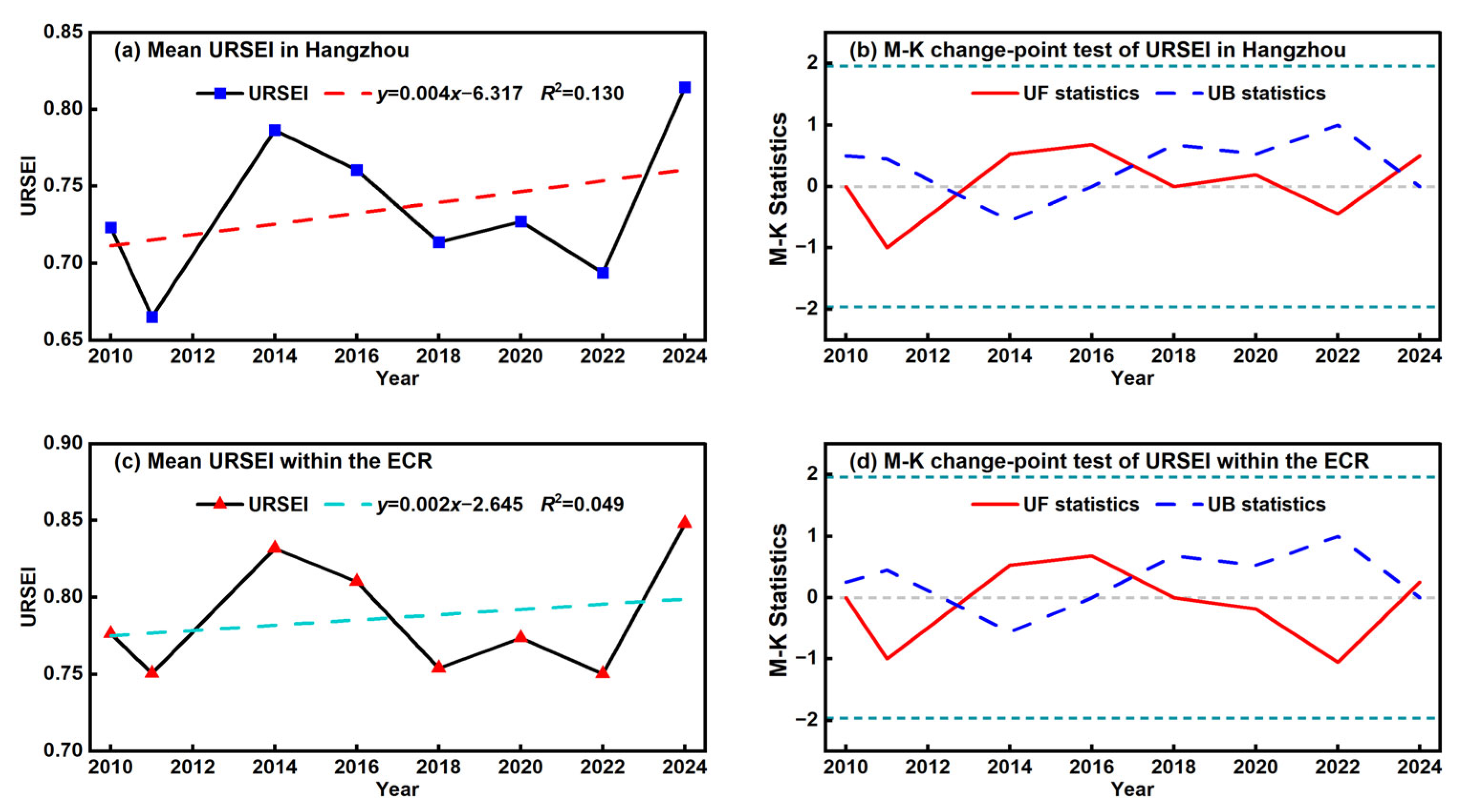
Using the annual mean URSEI values for Hangzhou, combined with the Mann–Kendall mutation test, temporal variations in ecological quality inside and outside the Ecological Conservation Redline (ECR) from 2010 to 2024 were analyzed (Figure 2).

As shown in Figure 2a, the mean URSEI value of Hangzhou ranged from 0.665 to 0.814 during the study period, indicating that overall ecological quality remained relatively high. Although fluctuations occurred across years, an overall upward trend was observed, with an average increase rate of 0.04 per decade. The temporal trajectory can be divided into three stages: an improvement phase from 2010 to 2014, a decline phase from 2014 to 2022, and a recovery phase from 2022 to 2024. This three-stage pattern reflects the combined influence of urban development, vegetation dynamics, and climatic conditions on the city’s ecological quality over time.

The Mann–Kendall mutation test results in Figure 2b show three intersection points between the UF and UB curves during 2010–2024, occurring in 2012–2014, 2016–2018, and 2022–2024. None of these intersections exceeded the confidence interval threshold, indicating that while temporal fluctuations in URSEI were present, no statistically significant abrupt changes occurred. This underscores the importance of interpreting the temporal variation as indicative trends rather than definitive improvements or degradations.

Within the ECR, the mean URSEI ranged from 0.750 to 0.848, consistently higher than the citywide average (Figure 2c). This suggests that ecological quality within protected areas remained superior to that of the broader urban region throughout the study period. Temporal variation within the ECR followed a generally similar pattern to that observed citywide, with a slight upward trend and an increase rate of 0.02 per decade.

Figure 2d presents the Mann–Kendall mutation test results for URSEI within the ECR. Similar to the citywide pattern, three UF–UB intersections were identified, but none exceeded the confidence interval threshold. These results indicate that ecological quality within the ECR remained relatively stable, without statistically significant abrupt changes, suggesting that protected areas maintained comparatively favorable ecological conditions during the study period.

Overall, the temporal analysis demonstrates that URSEI captures subtle variations in ecological quality over time, differentiates between protected and non-protected areas, and provides a robust framework for long-term monitoring of urban ecological dynamics under varying urbanization pressures.

4.2.2. Spatial Variation in Ecological Quality

(1)

Spatial Distribution Patterns

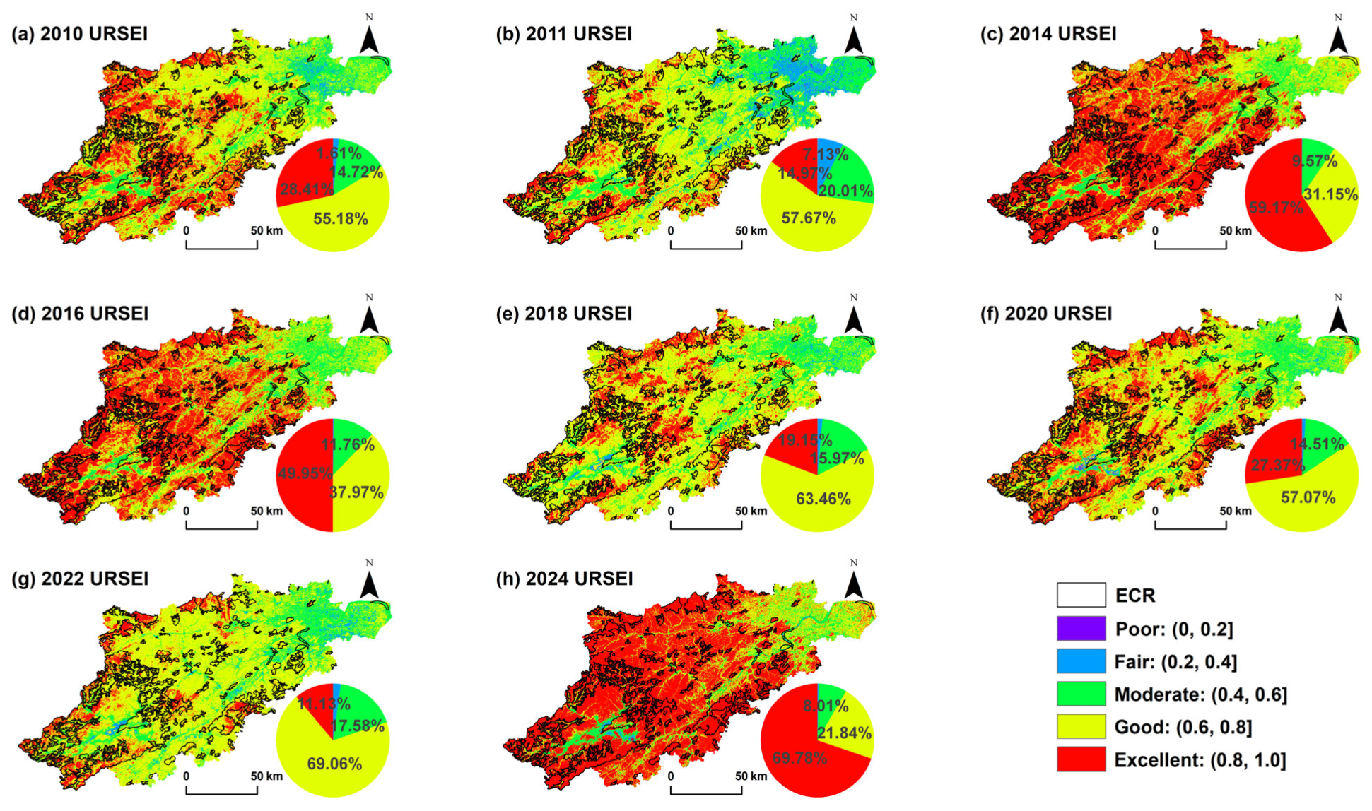
To examine spatial heterogeneity in ecological quality across Hangzhou, URSEI values were classified into five ecological quality levels. The spatial distribution patterns inside and outside the Ecological Conservation Redline (ECR) for 2010–2024 are shown in Figure 3.

As illustrated in Figure 3, ecological quality during 2010–2024 was predominantly categorized as “Good” and “Excellent,” with proportions ranging from 21.84% to 69.06% and 11.13% to 69.78%, respectively. High-quality areas were concentrated in the western, central, and southern hilly and mountainous regions, characterized by dense vegetation and relatively low urbanization.

“Moderate” ecological quality areas were mainly located in the northeastern plains (8.01–20.01%), while “Fair” quality areas were concentrated in the urbanized central regions (0.03–7.13%), with slightly higher proportions in 2011 and 2022. Poor-quality areas (<0.22%) were sparsely distributed in highly urbanized cores, highlighting localized ecological degradation associated with intensive urban development.

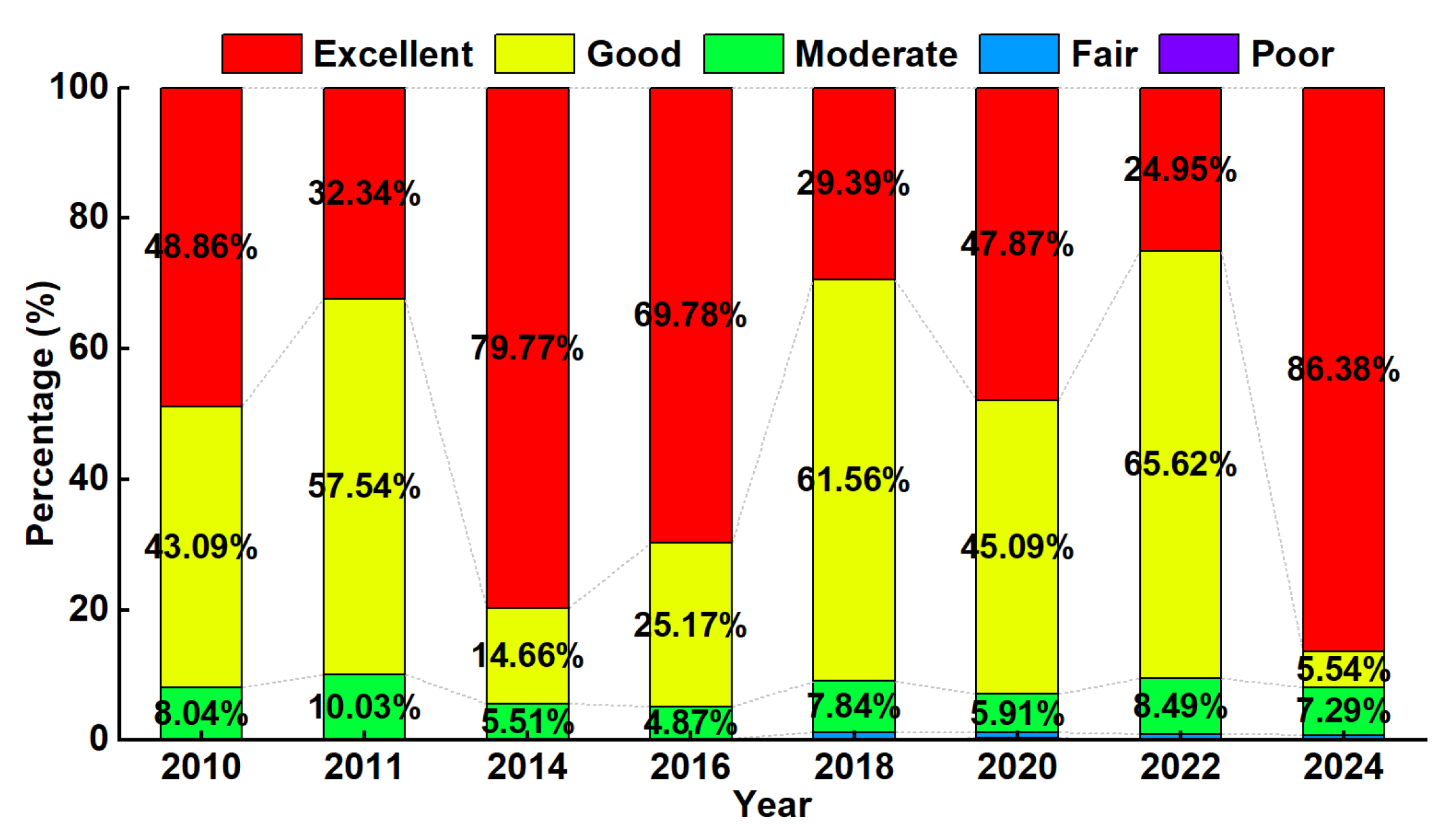
Within the ECR, “Excellent” and “Good” grades collectively accounted for 24.95–86.38% and 5.54–65.62% of the protected area, respectively (Figure 4), demonstrating that the ecological conservation redline effectively encompasses regions of high ecological quality and ecosystem service value.

These spatial patterns reveal clear ecological contrasts between vegetation-dominated regions and densely built-up urban cores: hilly and vegetated areas generally maintain higher ecological quality, whereas highly urbanized cores experience stronger anthropogenic pressures, underscoring the importance of integrating urbanization intensity into URSEI.

(2)

Temporal Trends

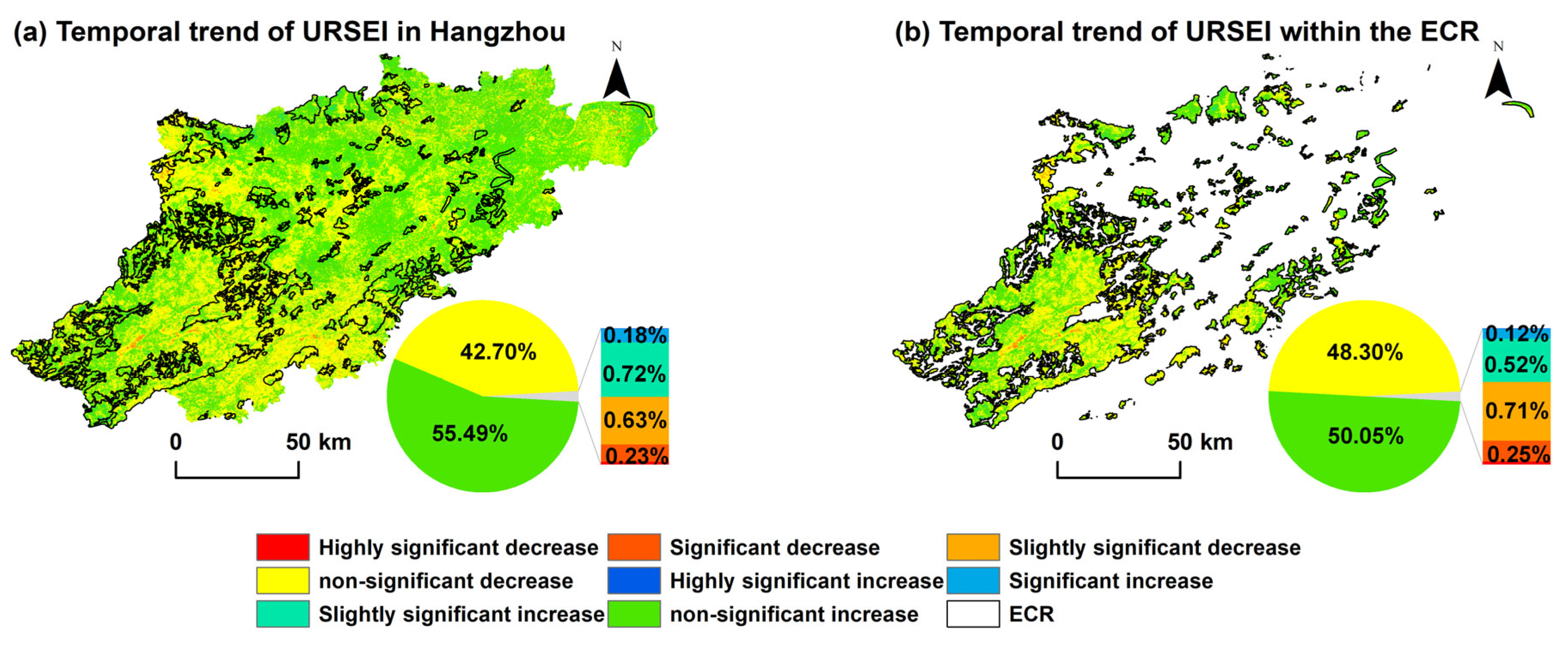
To further explore long-term temporal dynamics at the pixel level, Theil–Sen trend analysis combined with Mann–Kendall significance tests was applied to the URSEI time series. The resulting trend categories are presented in Figure 5.

As shown in Figure 5, 56.40% of Hangzhou exhibited an increasing trend, primarily in the central and northeastern plains. Among these, non-significant increases dominated, accounting for 55.49% of the area. Conversely, 43.60% of the study area showed a declining trend, mostly in southwestern Hangzhou, with non-significant decreases representing 42.70% of the area.

Within the ECR, trend patterns were broadly consistent with citywide results, with non-significant increases comprising 50.05% of the protected area. Overall, ecological quality remained spatially heterogeneous but statistically stable during the study period, with observed fluctuations interpreted as indicative trends rather than definitive improvements or degradations.

(3)

Trend Forecast

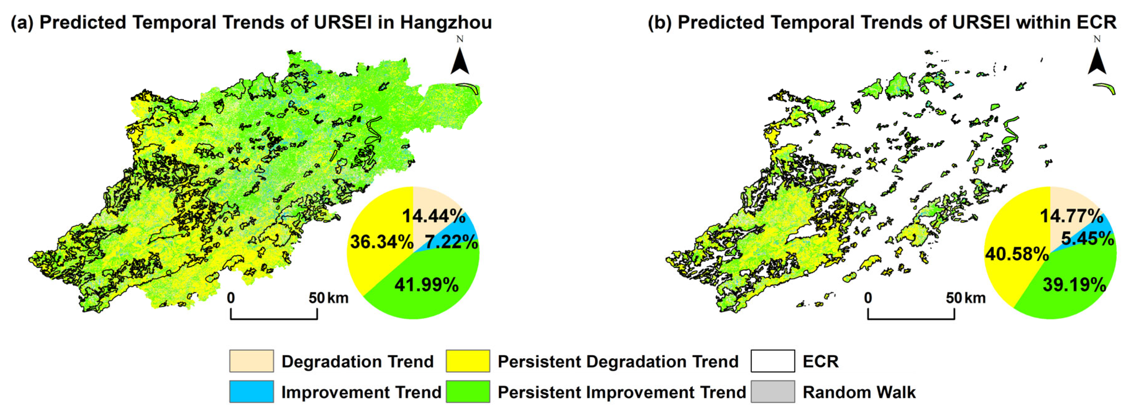
To assess future persistence of ecological quality trends, Theil–Sen slopes were combined with Hurst exponent forecasting to predict the expected trajectory of URSEI (Figure 6).

Predicted trends were categorized as follows: Degradation Trend (14.44%), Improvement Trend (7.22%), Random Walk (H = 0.5), Persistent Improvement Trend (41.99%), and Persistent Degradation Trend (36.34%). These trends were spatially heterogeneous: increasing and persistent improvement trends were concentrated in central, northeastern, and southwestern areas, while degradation trends were scattered throughout the city.

Within the ECR, Degradation and Persistent Degradation trends dominated, jointly accounting for 55.35% of the protected area, mainly around Thousand Island Lake in southwestern Hangzhou. These results indicate that future ecological interventions should prioritize these high-risk areas, and the forecasted trends should be considered indicative rather than deterministic predictions.

4.3. Analysis of Meteorological Drivers

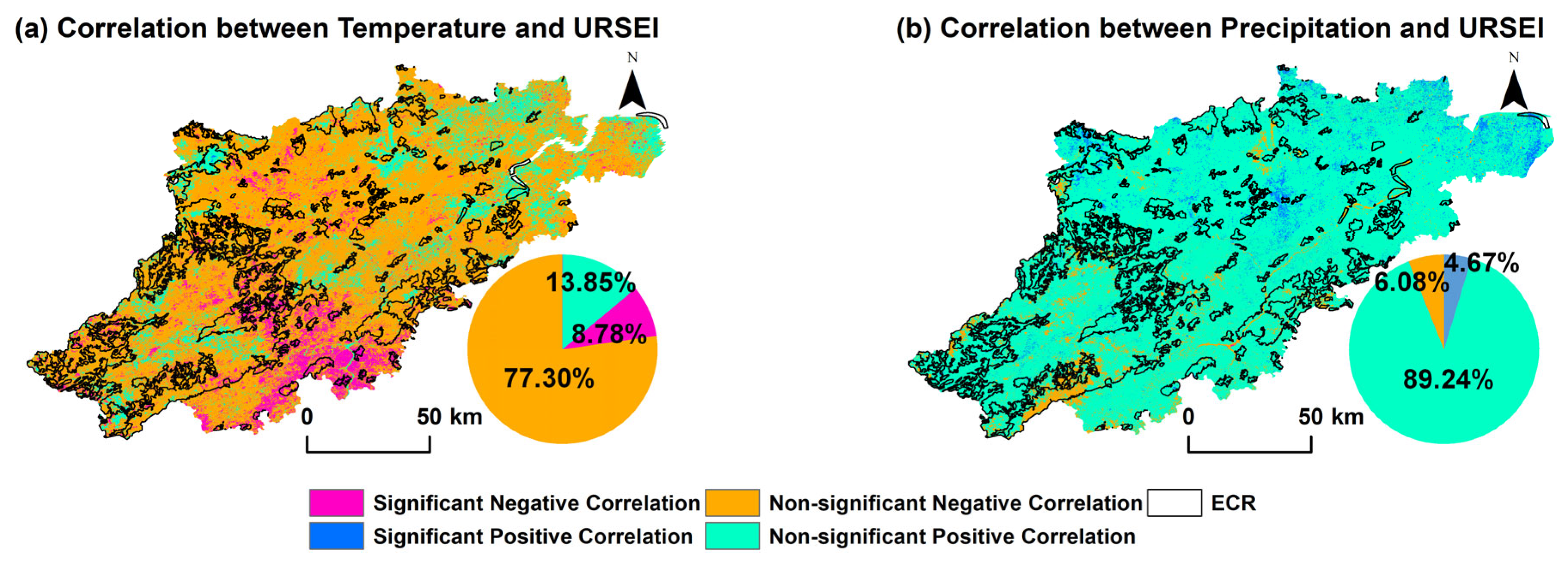
Urban ecological quality is strongly influenced by climatic and thermal conditions, particularly precipitation and temperature-related surface thermal stress, which affect vegetation growth, hydrological cycles, and overall ecosystem stability. To elucidate these relationships in Hangzhou, pixel-wise correlations were computed between annual URSEI values and corresponding annual precipitation and temperature-related thermal conditions represented by MODIS land surface temperature (LST) for 2010–2024. The spatial distribution of these correlations is illustrated in Figure 7.

As shown in Figure 7, temperature predominantly exhibits a negative correlation with URSEI, affecting 86.08% of total pixels. Of these, 8.78% show a statistically significant negative correlation, primarily located in southern Hangzhou and certain areas within the ECR. The remaining 77.30% represent non-significant negative correlations, largely concentrated in the western and central mountainous and hilly regions. This spatial pattern indicates that elevated temperatures generally impose stress on urban ecosystems by increasing evapotranspiration, water demand, and heat stress, thereby suppressing vegetation growth and ecosystem stability.

Conversely, precipitation shows a largely positive correlation with URSEI, covering 93.91% of pixels. Significant positive correlations account for 4.67% of the study area and are sporadically distributed in central and northern Hangzhou. Non-significant positive correlations account for 89.24%, mainly located outside the southwestern part of the city. Only 6.08% of pixels exhibit no clear correlation, predominantly within the ECR. The strong positive relationship between precipitation and URSEI highlights the critical role of water availability in regulating ecological quality and underscores the sensitivity of the urban ecosystem to hydrological conditions.

The spatial distribution of correlations suggests that densely vegetated hilly areas tend to show stronger positive associations with precipitation, whereas highly urbanized central plains exhibit more pronounced negative associations with temperature. This pattern implies that landscape context and urbanization intensity may influence the sensitivity of ecological quality to climatic drivers.

Overall, the proportion of pixels positively associated with precipitation was higher than that negatively associated with temperature-related thermal conditions, suggesting that precipitation showed a stronger association with URSEI among the climatic variables examined during the study period. These results imply that hydrological conditions play an important regulatory role in Hangzhou’s humid subtropical environment, and that urban management strategies should consider water conservation and vegetation restoration to help maintain ecosystem stability under climatic variability.

5. Discussion and Conclusions

5.1. Discussion

Urban ecological quality is a key component of sustainable urban development, directly influencing environmental health, ecosystem services, and residents’ well-being [38]. Under the dual pressures of rapid urbanization and climate change, urban ecosystems face increasingly complex and interrelated challenges [39]. Consequently, quantitative monitoring of urban ecological quality and the identification of the relative contributions of anthropogenic and climatic factors are essential for effective environmental management and sustainable urban planning.

As a rapidly urbanizing city in the Yangtze River Delta, Hangzhou offers an illustrative case for examining the interactions between urban expansion and ecological quality. In this study, the improved Urban Remote Sensing Ecological Index (URSEI) was applied to assess temporal and spatial variations in ecological quality, including within ECR-protected areas. By explicitly incorporating the Urbanization Index (UI) into the conventional RSEI framework, URSEI enhances the capacity of remote sensing ecological assessment to capture anthropogenic disturbance. Comparative analysis indicates that correlations between UI and URSEI consistently exceed those of thermal (LST) and dryness (NDBSI) indicators in most years, suggesting that urbanization intensity is more strongly associated with reduced URSEI values than thermal and surface dryness indicators in most years. This finding underscores the importance of including urbanization measures in ecological assessments of highly developed urban regions and aligns with prior studies emphasizing the ecological impact of urban expansion [40,41,42].

Integrating ECR boundaries into ecological quality monitoring provides a more targeted evaluation of conservation effectiveness. The results show that mean URSEI values within the ECR consistently exceed citywide averages, suggesting that redline areas maintained comparatively favorable ecological conditions during the study period. However, the absence of statistically significant improvement trends within the ECR implies that current protection measures primarily maintain baseline ecological conditions rather than promoting substantial enhancement, highlighting the need for adaptive management interventions.

Furthermore, by using annual mean ecological indicators derived from multi-temporal imagery during the peak vegetation season, the study minimizes short-term phenological variability and improves temporal representativeness compared with single-date RSEI approaches. This approach enhances the robustness of long-term monitoring and allows more reliable interannual comparison.

Despite the effectiveness of URSEI, several limitations should be acknowledged. First, the present study does not explicitly classify urban functional types or evaluate recognition accuracy across industrial areas, high-density built-up zones, low-rise built-up districts, and green or undeveloped spaces. Future studies should integrate high-resolution urban land-use, building morphology, or functional-zone datasets to further assess ecological responses across different urban form categories.

Second, the comparison between URSEI and RSEI in this study is primarily based on PCA contribution rates, component loadings, and internal correlation patterns rather than fully independent external validation. Although these analyses support the rationality and ecological interpretability of URSEI, future work should further evaluate the proposed index against temporally matched impervious surface products, land-cover change datasets, official ecological indicators, or field observations. In addition, the use of 2011 observations to represent the missing 2012 temporal node may introduce uncertainty into the continuity of the time series. Therefore, temporal interpretations around this substituted node should be regarded cautiously, and future studies should seek more complete annual observations or conduct sensitivity tests when suitable data are available.

Third, the meteorological driver analysis considered only temperature-related thermal conditions and precipitation, which cannot fully explain the complexity of urban ecological quality variation. Other factors, including land-use policy, population density, infrastructure expansion, vegetation restoration, water-body dynamics, air pollution, and local planning interventions, may also influence ecological conditions and should be incorporated in future multi-driver analyses. In addition, the climatic datasets used in this study were resampled to match URSEI’s 30 m spatial resolution for pixel-wise comparison. This spatial harmonization does not generate genuinely fine-scale climatic information and may introduce spatial uncertainty; future studies could employ high-resolution climate reconstruction or downscaling approaches to improve driver analysis.

Fourth, reliance on optical remote sensing data makes the framework vulnerable to cloud cover and adverse weather, suggesting that combining optical and SAR data in an active–passive synergistic monitoring approach could strengthen ecological quality assessment under complex atmospheric conditions. Overall, URSEI provides a robust and urbanization-aware framework that captures both natural and anthropogenic influences on urban ecological quality, offering actionable insights for urban environmental management and policy planning.

5.2. Conclusions

This study developed an improved Urban Remote Sensing Ecological Index (URSEI) by extending the conventional RSEI framework to explicitly incorporate urbanization intensity, thereby enhancing the capability of remote sensing ecological assessment in complex urban environments. Using Hangzhou as a case study, the URSEI framework was applied to evaluate ecological quality dynamics, forecast future trends, and assess climatic driving factors from 2010 to 2024. The main conclusions are summarized as follows:

(1) Rationality of URSEI: Throughout the study period, the contribution rate of the first principal component in URSEI was generally higher than that of RSEI, suggesting enhanced integration of ecological information across multiple environmental dimensions within the PCA framework. The strong negative correlation between the Urbanization Index (UI) and URSEI indicates that urbanization intensity exerts substantial ecological pressure, confirming the necessity of explicitly including urbanization in urban ecological quality assessment. The strong negative correlation between the Urbanization Index (UI) and URSEI indicates that urbanization intensity exerts substantial ecological pressure, confirming the necessity of explicitly including urbanization in urban ecological quality assessment. Nevertheless, the comparative advantage of URSEI over conventional RSEI is mainly supported by internal statistical behavior, component loadings, and ecological interpretability, and should be further validated using independent ecological, land-cover, or impervious surface datasets in future studies.

(2) Spatiotemporal Dynamics of Ecological Quality: From 2010 to 2024, 56.40% of Hangzhou exhibited increasing ecological quality trends, while 43.60% showed declining trends. However, the majority of these changes were statistically non-significant, indicating that the overall ecological quality of the city remained relatively stable over the study period. Within the ECR, ecological quality was consistently higher than the citywide average and followed temporal patterns broadly consistent with the overall urban area. These patterns indicate that ecological conditions vary across areas with different urbanization intensities and protection statuses, with hilly and vegetation-dominated regions generally maintaining better ecological quality than densely built-up urban cores.

(3) Climatic Driving Factors: Temperature-related thermal conditions, represented by land surface temperature, were generally negatively correlated with ecological quality, while precipitation exhibited predominantly positive correlations. Among the climatic variables examined, precipitation showed a stronger association with URSEI than temperature-related thermal conditions. The spatial variation in these correlations further indicates that ecological responses to climatic factors differ across protected and non-protected areas, emphasizing the need to jointly consider climate conditions and urbanization intensity when interpreting urban ecological dynamics.

Overall, the URSEI framework provides an urbanization-aware tool for long-term monitoring of urban ecological quality. It captures the combined effects of natural and anthropogenic drivers, reflects ecological differences across areas with contrasting urbanization intensities, and offers useful support for sustainable environmental management and urban planning in rapidly urbanizing regions. However, for direct planning applications, further testing at finer spatial units-such as individual buildings, industrial enterprises, residential developments, or urban subdistricts—is still needed to examine how URSEI responds to specific development types and functional land-use contexts. The study highlights that integrating urbanization indicators into composite ecological indices enhances the interpretability and management relevance of urban ecological assessments, while future applications should be strengthened through finer-scale validation and functional-zone analysis.

References

1. Almulhim, A.I.; Sharifi, A.; Aina, Y.A.; Ahmad, S.; Mora, L.; Filho, W.L.; Abubakar, I.R. Charting Sustainable Urban Development through a Systematic Review of SDG11. Nat. Cities 2024, 1, 677–685. [Google Scholar] [CrossRef]
2. Chaolin, G.U.; Weihua, G.; Helin, L.I.U. Chinese Urbanization 2050: SD Modeling and Process Simulation. Sci. China Earth Sci. 2020, 60, 1067–1082. [Google Scholar] [CrossRef]
3. Zhuang, Q.; Shao, Z.; Li, D.; Huang, X.; Altan, O. Isolating the Direct and Indirect Impacts of Urbanization on Vegetation Carbon Sequestration Capacity in a Large Oasis City: Evidence from Urumqi, China. Geo-Spat. Inf. Sci. 2023, 26, 379–391. [Google Scholar] [CrossRef]
4. Yu, J.; Li, X.; Guan, X.; Shen, H. A Remote Sensing Assessment Index for Urban Ecological Livability and Its Application. Geo-Spat. Inf. Sci. 2024, 27, 289–310. [Google Scholar] [CrossRef]
5. Huete, A.; Didan, K.; Miura, T.; Rodriguez, E.P.; Gao, X.; Ferreira, L.G. Overview of the radiometric and biophysical performance of the MODIS vegetation indices. Remote Sens. Environ. 2002, 83, 195–213. [Google Scholar] [CrossRef]
6. Pettorelli, N. The Normalized Difference Vegetation Index; Oxford University Press: Oxford, UK, 2013. [Google Scholar]
7. Qin, G.; Wang, N.; Wu, Y.; Zhang, Z.; Meng, Z.; Zhang, Y. Ecological Informatics Spatiotemporal Variations in Eco-Environmental Quality and Responses to Drought and Human Activities in the Middle Reaches of the Yellow River Basin, China from 1990 to 2022. Ecol. Inform. 2024, 81, 102641. [Google Scholar] [CrossRef]
8. Li, B.; Cheng, C.; Li, B. Integrating Multiple Environmental Variables to Identify Potential Urban Heat Island Risk Areas Based on the Maxent Model Island Risk Areas Based on the Maxent Model. Geo-Spat. Inf. Sci. 2025, 28, 3095–3109. [Google Scholar] [CrossRef]
9. Zhang, Y.; Shao, Z.; Xu, X.; Zhuang, Q. Quantifying Urban Vegetation Carbon Storage Using Seamless and Dense Time-Series Remote Sensing Data. Geo-Spat. Inf. Sci. 2025, 1–19. [Google Scholar] [CrossRef]
10. Manuvakola, A.; Ngolo, E.; Watanabe, T. Integrating Geographical Information Systems, Remote Sensing, and Machine Learning Techniques to Monitor Urban Expansion: An Application to Luanda, Angola. Geo-Spat. Inf. Sci. 2023, 26, 446–464. [Google Scholar] [CrossRef]
11. Zhang, H.; Ma, C.; Liu, P. Ecological Informatics Dynamic Evaluation of the Ecological Evolution and Quality of Arid and Semi-Arid Deserts in the Aibugai River Basin Based on an Improved Remote Sensing Ecological Index. Ecol. Inform. 2024, 82, 102727. [Google Scholar] [CrossRef]
12. Xu, H.; Wang, Y.; Guan, H.; Shi, T. Detecting Ecological Changes with a Remote Sensing Based Ecological Index (RSEI) Produced Time Series and Change Vector Analysis. Remote Sens. 2019, 11, 2345. [Google Scholar] [CrossRef]
13. Lu, F.; Zhang, C.; Cao, H.; Wang, X.; Zheng, T. Assessment of Ecological Environment Quality and Their Drivers in Urban Agglomeration Based on a Novel Remote Sensing Ecological Index. Ecol. Indic. 2025, 170, 113104. [Google Scholar] [CrossRef]
14. Pan, J.Y.; Wang, S.D.; Fan, Q.H. Assessment of Urban Ecological Quality Based on the Remote Sensing Green Index: A Case Study of Nanjing City. Remote Sens. Nat. Resour. 2024, 36, 88–95. [Google Scholar]
15. Sun, H.; Huang, M.; Lin, H.; Ge, Y.; Zhu, D.; Gong, D.; Altan, O. Spatiotemporal Dynamics of Ecological Environment Quality in Arid and Sandy Regions with a Particular Remote Sensing Ecological Index: A Study of the Beijing-Tianjin Sand Source Region. Geo-Spat. Inf. Sci. 2025, 1–20. [Google Scholar] [CrossRef]
16. Firozjaei, M.K.; Fathololoumi, S.; Weng, Q.; Kiavarz, M. Remotely Sensed Urban Surface Ecological Index (RSUSEI): An Analytical Framework for Assessing the Surface Ecological Status in Urban Environments. Remote Sens. 2020, 12, 2029. [Google Scholar] [CrossRef]
17. Bengal, W. Comparative Study on Remote Sensing-Based Indices for Urban Ecology Assessment: A Case Study of 12 Urban Centers in the Metropolitan Area of Eastern India. J. Earth Syst. Sci. 2024, 133, 100. [Google Scholar] [CrossRef]
18. Yang, X.; Meng, F.; Fu, P.; Zhang, J.; Liu, Y. Ecological Informatics Instability of Remote Sensing Ecological Index and Its Optimisation for Time Frequency and Scale. Ecol. Inform. 2022, 72, 101870. [Google Scholar] [CrossRef]
19. Guo, A.; Yue, W.; Yang, J.; Li, M.; Zhang, Z.; Xie, P.; Zhang, M.; Lu, Y.; He, T. Quantifying the Cooling Effect and Benefits of Urban Parks: A Case Study of Hangzhou, China. Sustain. Cities Soc. 2024, 113, 105706. [Google Scholar] [CrossRef]
20. Wang, R.; Liu, L.; Tao, Z.; Wan, B.; Wang, Y.; Tang, X.; Li, Y.; Li, X. Effect of Urbanization and Urban Forests on Water Quality Improvement in the Yangtze River Delta: A Case Study in Hangzhou, China. J. Environ. Manag. 2024, 351, 119980. [Google Scholar] [CrossRef]
21. Goward, S.N.; Xue, Y.; Czajkowski, K.P. Evaluating Land Surface Moisture Conditions from the Remotely Sensed Temperature/Vegetation Index Measurements: An Exploration with the Simplified Simple Biosphere Model. Remote Sens. Environ. 2002, 79, 225–242. [Google Scholar] [CrossRef]
22. Luo, Z.; Chai, B.; Wang, W. An Improved RSEI-Based Evaluation for Effective Forest Area by Integrating Forest Structure and Quality. Front. Environ. Sci. 2025, 13, 1580169. [Google Scholar] [CrossRef]
23. Wang, J.; Zhang, L.; Li, M. Monitoring Methods and Application of Urbanization Processes Based on Remote Sensing. J. Nanjing For. Univ. (Nat. Sci. Ed.) 2017, 41, 57–64. [Google Scholar]
24. Chander, G.; Markham, B.L.; Helder, D.L. Summary of Current Radiometric Calibration Coefficients for Landsat MSS, TM, ETM+, and EO-1 ALI Sensors. Remote Sens. Environ. 2009, 113, 893–903. [Google Scholar] [CrossRef]
25. Xu, H. A New Index for Delineating Built-up Land Features in Satellite Imagery. Int. J. Remote Sens. 2008, 29, 4269–4276. [Google Scholar] [CrossRef]
26. Rikimaru, A.; Roy, P.S.; Miyatake, S. Tropical Forest Cover Density Mapping. Trop. Ecol. 2002, 43, 39–47. [Google Scholar]
27. Huang, S.; Li, Y.; Hu, H.; Xue, P.; Wang, J. Assessment of Optimal Seasonal Selection for RSEI Construction: A Case Study of Ecological Environment Quality Assessment in the Beijing-Tianjin-Hebei Region from 2001 to 2020. Geocarto Int. 2024, 39, 2311224. [Google Scholar] [CrossRef]
28. Miao, W.; Chen, Y.; Kou, W.; Lai, H.; Sazal, A.; Wang, J.; Li, Y.; Hu, J.; Wu, Y.; Zhao, T. The HANTS-Fitted RSEI Constructed in the Vegetation Growing Season Reveals the Spatiotemporal Patterns of Ecological Quality. Sci. Rep. 2024, 14, 14686. [Google Scholar] [CrossRef]
29. Zhang, L.; Liang, T.; Wei, X.; Wang, H. An Improved Indicator Standardization Method for Multi-Indicator Composite Evaluation: A Case Study in the Evaluation of Ecological Civilization Construction in China. Environ. Impact Assess. Rev. 2024, 108, 107600. [Google Scholar] [CrossRef]
30. Du, Z.; Ji, X.; Liu, J.; Zhao, W.; He, Z.; Jiang, J. Ecological Health Assessment of Tibetan Alpine Grasslands in Gannan Using Remote Sensed Ecological Indicators Ecological Health Assessment of Tibetan Alpine Grasslands in Gannan Using Remote Sensed Ecological Indicators. Geo-Spat. Inf. Sci. 2025, 28, 246–264. [Google Scholar] [CrossRef]
31. Feng, X.; Tian, J.; Wu, J.; Wu, G.; Ren, Y.; He, C.; Bao, W.; Yu, T. Exploring the Spatio-Temporal Distribution Characteristics and the Impacts of Climate Change and Human Activities on Global Grassland Based on KNDVI. Environ. Res. 2025, 279, 121884. [Google Scholar] [CrossRef]
32. Wang, X.; Li, T.; Odion, H.; Rui, M.S. Spatio-Temporal Variability and Persistence of PM 2.5 Concentrations in China Using Trend Analysis Methods and Hurst Exponent. Atmos. Pollut. Res. 2022, 13, 101274. [Google Scholar] [CrossRef]
33. Abu, A.; Zakir, M.; Eyüp, S. Trend Analysis of Hydro-Meteorological Variables Using Mann-Kendall and Sen’s Slope with Standardization (SSS): Case Study of the Kızılırmak Catchment, Türkiye. Phys. Chem. Earth Parts A/B/C 2025, 141, 104115. [Google Scholar] [CrossRef]
34. Khan, A.; Hussain, S.; Bakhet, A.; Anwer, A.; Raza, S.M.M.; Ali, S.; Zakarya, M. Journal of Atmospheric and Solar-Terrestrial Physics Climate Time Series Variability Analysis of Islamabad Capital Territory Using Fractal Dimension and Hurst Exponent Methods. J. Atmos. Sol.-Terr. Phys. 2025, 267, 106406. [Google Scholar] [CrossRef]
35. Yin, Z.; Zhou, H.; Ke, P.; Wei, J. Time-Series SAR Scattering Coef Fi Cients over Woodland: Trend Analysis and Explainable Modelling. Front. Environ. Sci. 2025, 13, 1665409. [Google Scholar] [CrossRef]
36. Zhang, Q.; Cao, G.; Zhao, M.; Zhang, Y. KNDVI Spatiotemporal Variations and Climate Lag on Qilian Southern Slope: Sen–Mann–Kendall and Hurst Index Analyses for Ecological Insights. Forests 2025, 16, 307. [Google Scholar] [CrossRef]
37. Sanz, E.; Jos, J.; Saa-requejo, A.; Carlos, H.D.; Ruiz-ramos, M.; Rodr, A.; Tarquis, A.M. Clustering Arid Rangelands Based on NDVI Annual Patterns and Their Persistence. Remote Sens. 2022, 14, 4949. [Google Scholar] [CrossRef]
38. Estoque, R.C.; Wu, J. Science of the Total Environment The Resilience–Sustainability–Quality of Life Nexus. Sci. Total Environ. 2024, 912, 169526. [Google Scholar] [CrossRef]
39. Zhang, X.; Deng, G.; Chen, L.; Abbass, K. Sustainable Development and Climate Action: The Role of Tax Policy and Innovation. J. Environ. Manag. 2025, 389, 126091. [Google Scholar] [CrossRef]
40. Zhang, X.; Fan, H.; Sun, L.; Liu, W.; Wang, C.; Wu, Z. Identifying Regional Eco-Environment Quality and Its Influencing Factors: A Case Study of an Ecological Civilization Pilot Zone in China. J. Clean. Prod. 2024, 435, 140308. [Google Scholar] [CrossRef]
41. Singh, S.; Shukla, A.; Jain, K. Remote Sensing Applications: Society and Environment Assessing the Urbanization-Induced Impact on Environmental Parameters of a City from a Remote-Sensing Perspective. Remote Sens. Appl. Soc. Environ. 2025, 34, 101169. [Google Scholar] [CrossRef]
42. Wang, Z.; Yu, Y.; Zhou, R. A Longitudinal Exploration of the Spatiotemporal Coupling Relationship and Driving Factors between Regional Urban Development and Ecological Quality of Green Space. Ecol. Indic. 2024, 164, 112134. [Google Scholar] [CrossRef]
Figure 1. Geographic Location and Land Cover Types of Hangzhou. (a) Location of Zhejiang Province within China; (b) location of Hangzhou City within Zhejiang Province; (c) elevation distribution of Hangzhou City; (d) land use types of Hangzhou City, including waters, forest, shrub, crops, and town areas.
Sustainability 18 05394 g001
Figure 2. Trend of mean URSEI and M-K change-point test inside and outside the ECR in Hangzhou.
Sustainability 18 05394 g002
Figure 3. Spatial distribution of URSEI grades inside and outside the ECR in Hangzhou from 2010 to 2024.
Sustainability 18 05394 g003
Figure 4. Proportion of ecological quality grades within the ECR.
Sustainability 18 05394 g004
Figure 5. Temporal trends of ecological quality inside and outside the ECR in Hangzhou from 2010 to 2024.
Sustainability 18 05394 g005
Figure 6. Predicted temporal trends of ecological quality inside and outside the ECR in Hangzhou.
Sustainability 18 05394 g006
Figure 7. Spatial distribution of correlations between URSEI and temperature and precipitation from 2010 to 2024.
Sustainability 18 05394 g007