Review

Artificial Intelligence in Atmospheric Composition Studies for Sustainable Air Quality Management: Spatiotemporal Concentration Forecasting and Emission Inference from Mobile and Point Sources

by
Anna Korzeniewska
and
Katarzyna Szramowiat-Sala
*
Faculty of Energy and Fuels, AGH University of Krakow, Al. A. Mickiewicza 30, 30-059 Kraków, Poland
*
Author to whom correspondence should be addressed.
Sustainability 2026, 18(10), 4838; https://doi.org/10.3390/su18104838
Submission received: 27 February 2026 / Revised: 8 May 2026 / Accepted: 11 May 2026 / Published: 12 May 2026

Abstract

Air pollution remains a major challenge for sustainable development because of its impacts on human health, ecosystems, and climate. At the same time, the rapid growth of environmental data and advances in artificial intelligence (AI) have created new opportunities for atmospheric composition research and air-quality management. This review examines AI applications in atmospheric composition studies, focusing on two related but distinct tasks: (i) spatiotemporal forecasting of pollutant concentrations and (ii) emission inference from mobile and point sources. It emphasizes the fundamental differences between these tasks in terms of data requirements, model design, and physical interpretability. A synthesis of representative studies published between 2018 and 2025 is provided, covering machine learning and deep learning approaches for air-quality prediction and emission characterization. Recent foundation-style architectures and global AI weather models introduced in late 2025 and early 2026 further demonstrate the growing role of large-scale spatiotemporal learning in atmospheric and environmental prediction. Particular attention is given to hybrid and physics-informed models that aim to connect data-driven methods with atmospheric processes. The review also discusses major methodological challenges, including data representativeness, sensor uncertainty, spatial transferability, and model generalization under nonstationary conditions. It highlights the importance of leakage-resistant evaluation, appropriate temporal and spatial splitting strategies, and the roles of interpretability and uncertainty quantification in physically meaningful atmospheric modelling. From a sustainability perspective, these AI approaches can support more reliable monitoring, improved emission assessment, and better-informed strategies for air-pollution mitigation.

1. Introduction

Environmental monitoring and prediction in atmospheric sciences are constrained by nonlinear interactions, multiscale feedback (from street-canyon turbulence and boundary-layer mixing to synoptic forcing), and stochastic variability in meteorology and emissions. Observed air-pollution fields are emergent outcomes of coupled processes: (i) source terms (emissions from mobile and stationary sources), (ii) transport and mixing (advection, diffusion, turbulence, boundary-layer evolution), (iii) chemical transformation (gas-phase and multiphase chemistry), and (iv) removal (dry/wet deposition). In standard Eulerian formulations, these mechanisms are represented by the advection–diffusion–reaction equation with source and sink terms, which provides a physical “spine” for interpreting what data-driven models should learn rather than merely predict [1]. These properties generate heterogeneous, irregular, and often high-frequency datasets that challenge classical modelling toolchains—especially when the system is nonstationary, measurements are incomplete, and source strengths evolve rapidly in time [2].
Artificial intelligence provides complementary methods for learning nonlinear mappings from environmental data. Modern deep learning architectures reframe atmospheric observations as structured objects: convolutional neural networks (CNNs) for spatial fields, recurrent and temporal-convolution models for sequences, attention mechanisms for long-range dependencies and graph neural networks (GNNs) for irregular monitoring networks [3,4]. A critical distinction—often blurred in applied AI studies—is the difference between forecasting concentrations at receptors and estimating emissions from sources. Concentration forecasting predicts what monitoring stations measure given meteorology, prior concentrations, and proxies for emissions. In contrast, emission estimation is an inverse problem: the source term is inferred indirectly through transport, mixing, and chemistry, typically requiring additional physical constraints, forward models (i.e., numerical operators that simulate how emissions propagate through atmospheric transport, mixing, and chemical transformation to produce observable concentrations), and uncertainty-aware inversion or data assimilation frameworks. In practice, emission inversion is affected by multiple sources of uncertainty, including transport model error, chemical mechanism uncertainty, and assumptions embedded in prior emission inventories. Treating these as interchangeable can lead to scientifically misleading claims [5,6]. At the same time, physically based and measurement-driven approaches—including experimental emission characterization and receptor-oriented source apportionment—provide direct insight into emission processes and source contributions, highlighting aspects of system behaviour that may not be fully captured by data-driven models alone [7,8]. AI-based hybrid modelling is increasingly adopted when physical consistency must be maintained while enabling faster inversion or higher-resolution state reconstruction [9,10]. In such workflows, machine learning (ML) augments or accelerates physics-based atmospheric models through neural surrogates, dispersion emulators, or learned parameterizations. Recent foundation-style architectures further demonstrate that attention- and graph-based models can capture long-range spatiotemporal dependencies at global scales. However, their application to air-quality problems requires adaptation to account for the central role of emissions and atmospheric chemistry [11,12]. Recent foundation-style atmospheric AI systems further demonstrate that attention- and graph-based architectures can capture long-range spatiotemporal dependencies at continental and global scales [12,13]. Examples include large-scale forecasting systems such as GraphCast and the Aurora foundation model, which illustrate the growing role of foundation-style AI in Earth-system and environmental prediction [12,13]. Related developments continued into late 2025 and early 2026, reflecting the rapid expansion of large-scale AI frameworks for weather, climate, and atmospheric forecasting [14,15]. However, their application to air-quality problems still requires adaptation to account for the central role of emissions, chemical transformation, and source-term variability. Strong predictive scores alone are not sufficient for atmospheric science. Reliable evaluation requires leakage-resistant evaluation strategies, that is, validation designs that minimize information leakage between training and test data by respecting temporal order and spatial dependence, such as blocked timesplits, rolling-origin validation, and spatial hold-outs, rather than naive random splits that inflate performance through spatiotemporal dependence [16]. The risk of opaque model behaviour should likewise be addressed through explainable AI (XAI) and calibrated uncertainty quantification, testing whether models rely on physically meaningful drivers (e.g., meteorological forcing, emission proxies, and chemical regimes) rather than spurious correlations.
Accordingly, this review provides a process-anchored synthesis of AI methodologies for atmospheric composition studies, focusing on (i) spatiotemporal forecasting of pollutant concentrations and (ii) emission inference from mobile and stationary sources treated as dynamic source terms. A central methodological contribution of this review is the distinction between concentration prediction and source-term inference. The review demonstrates that these tasks are fundamentally different in terms of physical interpretation, modelling assumptions, validation requirements, and uncertainty treatment. Throughout the review, this distinction serves as the main organizational and methodological principle for interpreting AI applications in atmospheric composition studies. Building on the advection–diffusion–reaction framework, the review relates AI approaches to atmospheric processes and data structure, and critically examines the transition from classical machine learning baselines to deep learning and hybrid physics-consistent models. Beyond performance comparisons, the review emphasizes methodological conditions required for credible inference, including leakage-resistant evaluation, robustness under spatiotemporal dependence and distribution shift, and the role of interpretability and uncertainty quantification in assessing physical plausibility.
In this sense, the review positions AI not only as a predictive tool, but as a scientific instrument for atmospheric composition, supporting physically meaningful emission characterization, defensible forecasts, and reliable decision-making in sustainable air-quality management.

2. From Classical to Modern AI

The physical framing introduced in Section 1 implies a simple but consequential point: in atmospheric composition, predictive models are not interchangeable black boxes. A method is only meaningful relative to the task it serves—forecasting concentrations at receptors versus inferring source terms—and relative to the process pathways through which emissions, transport/mixing, and chemistry jointly generate the observed fields [1,2,5,6]. This perspective motivates methodological progression that is common in practice but often blurred in the literature: transparent baselines and exploratory structure discovery first, followed by increasingly expressive models that can represent spatiotemporal dependence and heterogeneous inputs without sacrificing credible evaluation.
Classical machine learning models remain valuable in this context because they provide strong, interpretable reference points and help diagnose regime structure, nonstationarity, and data limitations before deep architectures are introduced [17,18,19,20,21]. Modern deep learning families extend this toolset by learning representations directly from structured atmospheric data—gridded fields, multi-station sequences, and networked observations—thereby capturing spatial gradients, temporal persistence, and long-range dependencies that are difficult to encode by hand [22,23,24,25,26,27].
To reduce ambiguity in terminology, we distinguish three complementary approaches to integrating physical knowledge with AI. Hybrid models couple data-driven components with physical models (e.g., CTM, dispersion, or CFD), typically using AI for surrogate modelling, bias correction, or computational acceleration. Physics-informed approaches embed physical constraints directly into the learning process, for example through loss functions, governing equations, or conservation laws. Physics-consistent approaches, in contrast, do not enforce constraints during training but ensure that model outputs remain physically plausible and interpretable, for example through post hoc validation or feature attribution.
Because the same datasets can support very different claims depending on how models are trained, validated, and interpreted, the methodological discussion in this section also keeps evaluation practice in view. Approaches that ignore spatiotemporal dependence can overstate generalization through spatial/temporal leakage, whereas blocked and time-aware splitting better reflect the conditions under which air-quality models are expected to operate [16,28].

2.1. Structure of AI-Based Modelling in Atmospheric Studies

Artificial intelligence is an umbrella term for computational methods that perform tasks typically associated with intelligent decision-making, such as prediction, pattern recognition, optimization, and control. Machine learning is a major subset of AI in which models learn statistical relationships from data rather than being fully specified by explicit rules. Within ML, artificial neural networks (ANNs) constitute a family of models built from layers of interconnected computational units. Deep learning (DL) refers to neural networks with multiple stacked layers that learn hierarchical representations directly from data (“feature learning”), thereby reducing the need for hand-crafted descriptors [17,22].
These distinctions matter operationally in atmospheric and environmental applications because they map onto data structure and scientific objectives. In this review, “classical ML” denotes feature-based models such as linear and regularized regression, support vector machines, random forests, and gradient-boosted trees, which typically rely on engineered predictors and careful preprocessing [17,18,19,20]. Classical workflows are often complemented by unsupervised structure discovery (e.g., dimensionality reduction and clustering) to identify circulation or pollution regimes, detect outliers, and support stratified evaluation [21].
By contrast, “deep learning” is used when the information content is distributed across space, time, and networks—such as gridded meteorological fields, satellite products, images, or multi-station sequences—so the model must learn spatial, temporal, or relational structure directly. Representative DL families include convolutional neural networks for spatial fields, recurrent sequence models such as LSTM/GRU for temporal dynamics, transformer-style attention mechanisms for long-range dependencies and heterogeneous data fusion, and graph neural networks for irregular monitoring networks and connectivity defined by geography or flow-related relationships [23,24,25,26,27]. “Modern AI” primarily denotes DL and hybrid, physics-consistent approaches, including physics-informed and theory-guided learning, whereas “classical AI/ML” denotes feature-based baselines and unsupervised structure discovery used for transparent benchmarking and regime diagnosis [9,10].
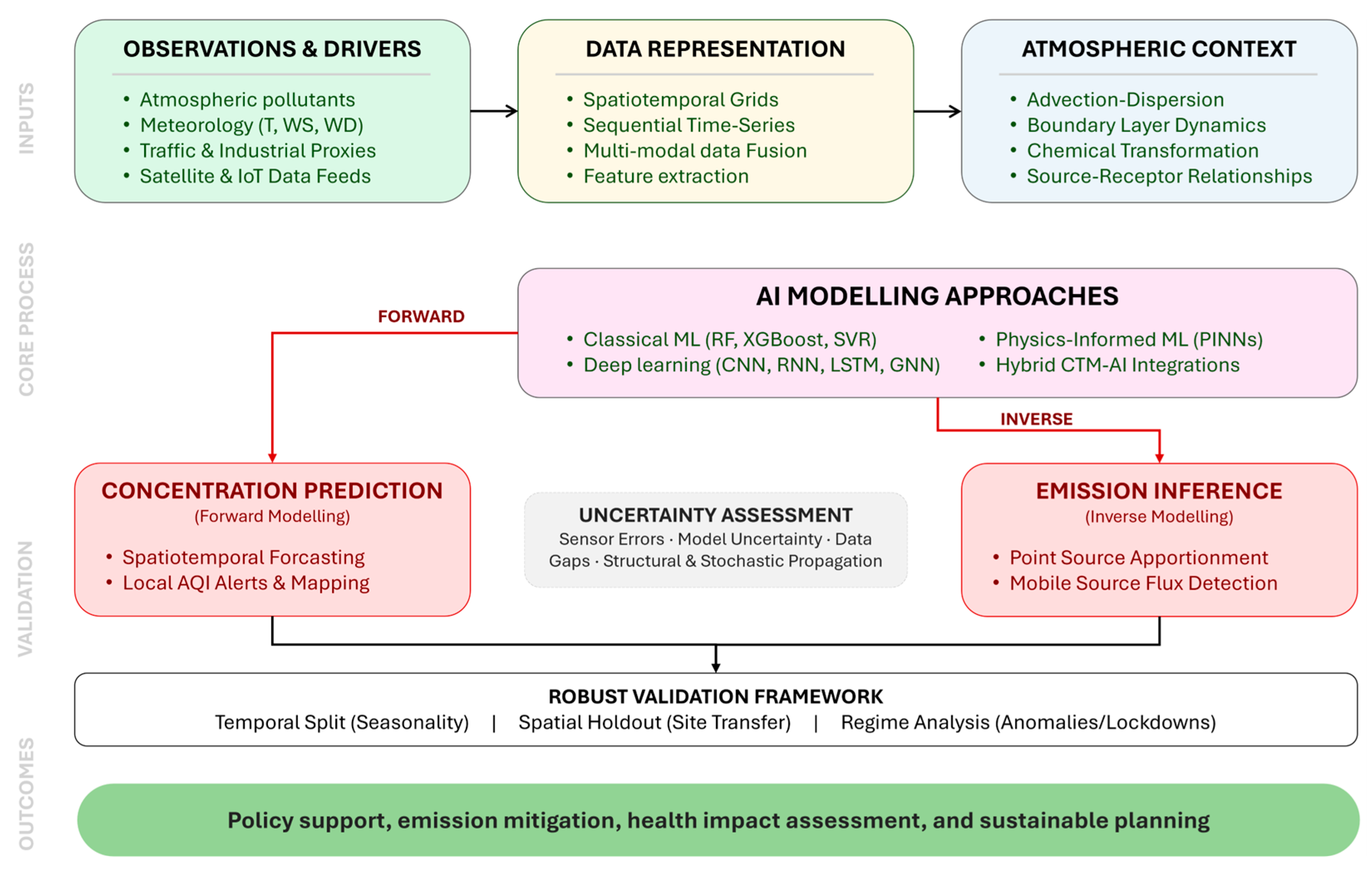
To organize these relationships in a physically and methodologically consistent way, we introduce a conceptual framework that links data, processes, and modelling approaches in atmospheric AI (Figure 1). The framework distinguishes between forward (concentration prediction) and inverse (emission inference) problems, emphasizing their different data requirements, modelling assumptions, and levels of uncertainty. It further incorporates validation strategies addressing temporal, spatial, and regime-dependent generalization, as well as uncertainty assessment related to sensor errors, data limitations, and model structure. The framework illustrates how combining data-driven and physics-informed approaches enables more reliable air quality forecasting, emission characterization, and supports decision-making for sustainable air quality management.
Building on this structured view, the following section focuses on practical modelling workflows used in atmospheric AI studies. We emphasize how data representation, model selection, and validation design jointly determine whether a model provides physically meaningful and generalizable results. This transition from conceptual organization to applied methodology is essential for interpreting reported model performance and for ensuring credible deployment in air-quality applications.

2.2. AI-Based Data-Science Procedure for Environmental and Atmospheric Data

The terminology in Section 2.1 clarifies what we mean by classical ML and modern deep learning families, but credible atmospheric results depend at least as much on the end-to-end data-science procedure as on the model family itself. This is particularly true for air-quality applications, where observations are heterogeneous (stations, satellites, low-cost sensors, model outputs), the system is strongly nonstationary (seasonality, regime shifts, abrupt emission changes), and spatiotemporal dependence can inflate performance when train/test separation is not designed to prevent leakage. For dependent ecological and environmental data, validation strategies should be matched to the dependence structure, with blocked and grouped splits preferred over naive random sampling when the goal is generalization across time, space, or regimes [16,28]. In this review, we use an end-to-end workflow lens—spanning problem definition, data collection, preprocessing, feature construction and split design, modelling and tuning, and finally validation and reporting—to interpret and compare studies and to identify common failure modes.
A defensible procedure begins by defining the scientific task and the intended generalization target, because these choices determine what constitutes a meaningful test. For example, receptor-side concentration forecasting, spatial reconstruction, exceedance detection, and source characterization correspond to different targets and different tolerances for error and uncertainty. Clear task specification also makes inputs interpretable in physical terms, distinguishing drivers (meteorology, boundary-layer structure) from proxies (activity indicators) and clarifying whether the analysis is intended to generalize across locations, across seasons, or across emission regimes. Comparative studies that evaluate ML models under real-world air-quality constraints highlight that differences in data handling and evaluation design can dominate differences between algorithms, including the apparent performance gap between classical machine learning and deep learning models [29,30].
Preprocessing then converts raw environmental observations into analysis-ready data, and in air-quality contexts, this step often controls the reliability of downstream conclusions. Missingness is not just an inconvenience: recent studies show that the choice of imputation strategy can materially change predictive performance and should be treated as an explicit modelling decision rather than clerical cleanup [31,32]. In addition, outlier handling and de-spiking are essential for heterogeneous sensor networks, particularly where low-cost measurements introduce spikes and artefacts that a model could otherwise learn as “signal” [33]. For short-term policy and attribution questions, it can also be important to reduce the risk that models succeed primarily by learning calendar regularities (diurnal/weekly/seasonal cycles) rather than event-scale dynamics; refined weather-normalization strategies are explicitly designed to address this failure mode [34]. When decomposition-based feature construction is used, it should be implemented in a way that respects the train/test boundary, because several decomposition pipelines can inadvertently leak future information if applied across the full dataset before splitting [35]. Decomposition-and-ensemble pipelines have nevertheless shown value when implemented carefully, helping separate temporal components before prediction [36].
Feature construction and data splitting are best treated as a coupled design step. Air-quality predictors commonly include lags, rolling aggregates, and meteorological conditioning variables, but the evaluation split must reflect the intended deployment scenario. Random splits are rarely appropriate for atmospheric time series and station networks because nearby samples are dependent; blocked time-splits, rolling-origin validation, and spatial hold-outs (e.g., leave-location-out) provide more realistic tests of generalization [16,28]. A practical template for leakage-resistant evaluation with sequence learners is provided by applications that combine recurrent models with blocked cross-validation in other environmental process settings, illustrating how to keep model selection and assessment aligned with dependence structure [37]. For atmospheric studies that make claims about transfer across stations or regions, spatial hold-outs and regime-aware reporting are particularly important, because average performance can hide systematic failures under episodes and extremes [30,34].
Within this procedure, model choice becomes interpretable rather than fashionable. Classical ML models and tree ensembles remain strong baselines for engineered predictors and are widely used to improve deterministic forecast products and to quantify performance trade-offs under realistic operational constraints [29,30]. Deep learning architectures are most justified when information is distributed across space, time, and networks—such as gridded fields, multi-station sequences, or irregular sensor layouts—because they can learn structure that is difficult to encode manually. Representative examples include CNN–LSTM hybrids for spatiotemporal prediction [38], transfer-oriented sequence models for new monitoring sites [39], and graph-based approaches that model inter-station coupling for air-quality forecasting [40,41,42]. Hybrid and physics-consistent approaches can further strengthen robustness under regime shifts by incorporating physically motivated constraints or coupling learned components to mechanistic modelling elements; these strategies are particularly relevant when extrapolation is required beyond the regimes represented in training data [21,22].
Model fitting should be paired with transparent hyperparameter tuning and regularization, because nonstationarity and dependence can enable subtle overfitting even when headline skill appears strong. Reproducible tuning workflows increasingly use cross-validation combined with Bayesian hyperparameter optimization in environmental classification and modelling contexts, and similar ideas have been used for sensor-correction applications where model settings strongly affect performance [43,44]. To preserve credibility, tuning should be performed strictly within training data, with the final test set reserved for a single unbiased assessment under the target split design [28,29].
Finally, evaluation and reporting translate scores into atmospheric meaning. Metrics should match the task (e.g., RMSE/MAE and bias for concentration prediction; classification metrics for exceedance detection), and reporting should be stratified by pollutant, site type, lead time, and regime, where possible, because averaged metrics can mask breakdown during high-impact episodes [30,34]. When interpretability tools are used, they should be treated as diagnostic instruments rather than decorations: they should test whether the model relies on physically plausible drivers and whether conclusions remain stable under perturbations, missingness, and drift [45]. Taken together, these end-to-end considerations provide a consistent basis for comparing studies reviewed later in this paper and for distinguishing genuine generalization from results inflated by leakage or dataset-specific artefacts [16,28,35]. For operational settings, they should be extended with post-deployment monitoring (drift detection, recalibration triggers, and periodic revalidation) to prevent silent performance degradation. This workflow perspective provides the methodological backbone for interpreting the studies reviewed in subsequent sections.

2.3. From Classical ML to Modern DL: Architectures Matched to Data Structure

In this section, we focus not on exhaustive model taxonomy but on how architectural choices align with the structure of atmospheric data and the nature of the prediction or inference task. The central methodological point of Section 2 is that model families are tools whose usefulness depends on the geometry of the data and the type of atmospheric signal one expects the model to represent. In air-quality applications, this geometry is rarely “tabular” in a strict sense: information is distributed across space (fields and gradients), time (persistence and delayed responses), and networks (irregular station layouts and inter-site coupling). Modern deep learning families are therefore best understood as architectures that impose inductive biases aligned with these structures, rather than as universally superior replacements for classical ML. Classical machine learning models remain indispensable as transparent reference points and strong performers when predictors are well engineered (meteorology, emissions proxies, lags, rolling aggregates) and when interpretability or limited data dominate. Linear and regularized regression, support-vector methods, random forests, and gradient-boosted trees are widely used because they provide robust baselines and expose whether performance gains from deep models reflect genuine spatiotemporal learning or simply improved fitting of seasonality and covariate interactions [17,18,19,29,30]. Unsupervised structure discovery (e.g., dimensionality reduction and clustering) can further reveal regime structure and guide stratified analysis, supporting physically interpretable comparisons across methods. Deep learning architectures become most defensible when the predictive content is embedded in structured inputs that are difficult to compress into hand-crafted features without losing key information. For spatially structured data—gridded meteorology, satellite products, or model fields—convolutional neural networks provide an inductive bias that matches local spatial coherence and multiscale patterns. CNN-based components are therefore natural for learning spatial gradients and plume-like morphology when inputs can be represented on a grid, and CNN–sequence hybrids are frequently used when both spatial and temporal dependencies are important [22,23,38].
When temporal dependence is central, recurrent sequence models such as LSTM/GRU provide a direct mechanism for representing persistence and delayed responses associated with transport, boundary-layer evolution, and chemistry. In air-quality forecasting, sequence learners are commonly applied as site-level predictors or as temporal modules inside spatiotemporal systems, and transfer-oriented variants have been proposed to support prediction at newly deployed stations with limited historical data [24,25,39]. Temporal convolutional designs can provide similar benefits while offering stable training and parallelism and are often used as alternatives to recurrent modules in modern pipelines [3,46].
Attention-based models (transformers) extend sequence modelling by learning flexible, content-dependent interactions across long horizons and heterogeneous inputs. This is attractive when relevant context spans multiple time scales (episode build-up versus synoptic transitions) and when multi-source fusion is required (stations + satellite + reanalysis + proxies). In atmospheric applications, attention mechanisms can help represent long-range dependence, but they also increase model capacity and therefore require disciplined study design and careful interpretation of what signals the model uses in practice [26]. In this review, transformers are treated as a powerful representational family whose value depends on whether they capture physically plausible dependencies rather than shortcut correlations [47].
For irregular monitoring networks, graph neural networks provide an inductive bias closer to how air-quality observations are collected: nodes (stations/sensors) connected by edges that encode proximity, similarity, or transport-informed coupling. In GNNs, each node iteratively aggregates information from its neighbours through a learned message-passing mechanism, updating its hidden representation based on both local features and the graph structure. This allows the model to capture spatial dependencies defined by network topology rather than purely Euclidean distance [27,48]. Graph-based forecasting explicitly models inter-station dependence and can incorporate heterogeneous node attributes (site type, elevation, local land use) as well as dynamic meteorological context. Recent studies demonstrate attentive and spatiotemporal graph designs for air-quality prediction and spatial inference on networks that do not align with regular grids [27,40,41,42]. In atmospheric applications, GNNs are particularly suitable where station density is uneven and where pollutant transport relationships are not strictly distance-based but influenced by local dynamics and connectivity patterns.
Viewed together, modern DL should not be framed as a replacement for classical ML but as an expansion of representational capacity that becomes useful when the data structure demands it. Classical baselines remain essential for transparency and for anchoring claims, while CNN/sequence/attention/graph architectures become most valuable when they are selected to match the underlying space–time–network structure of the observations and when their learned dependencies can be defended as physically meaningful rather than incidental [17,18,19,20,21,22,23,24,25,26,27].
A consistent observation across atmospheric and environmental studies is that performance differences between classical machine learning models and deep learning approaches are highly task- and data-dependent rather than universal. Classical models such as random forests and gradient-boosted trees often provide competitive or superior performance when predictors are well engineered, datasets are moderate in size, and the dominant signal can be captured through aggregated meteorological and proxy variables. In such settings, their robustness, lower variance, and interpretability make them strong baselines and, in some cases, preferred operational choices. By contrast, deep learning architectures tend to outperform classical models when predictive information is distributed across structured inputs—such as spatial fields, temporal sequences, or monitoring networks—and when the task requires learning interactions that are difficult to encode explicitly. This includes spatiotemporal forecasting, multi-source data fusion, and transfer across locations with heterogeneous conditions. However, these gains are contingent on sufficient data volume, careful regularization, and leakage-resistant evaluation; otherwise, deep models may overfit or exploit spurious correlations while appearing to achieve high accuracy.
Importantly, reported performance improvements should be interpreted with caution in the presence of spatiotemporal dependence. Studies using random train/test splits frequently overestimate the advantage of deep learning, whereas more realistic validation strategies (e.g., temporal blocking or spatial hold-outs) often reduce or eliminate apparent performance gaps. For this reason, classical and deep models should be viewed as complementary rather than hierarchical, with their relative performance determined by data structure, task definition, and evaluation design rather than by model complexity alone.
Model suitability in atmospheric applications is therefore determined not only by data structure, but also by the underlying physical processes that generate the observed signals. Spatial models such as CNNs are most effective when pollutant fields exhibit coherent gradients or plume-like structures but may struggle when transport is dominated by highly irregular or non-local dynamics. Sequence models (LSTM/GRU) are well suited to processes with temporal persistence and delayed responses, yet their performance can degrade under regime shifts, abrupt emission changes, or nonstationary forcing. Attention-based models and transformers can capture long-range and multi-scale dependencies, but their flexibility increases the risk of learning spurious correlations if not constrained by appropriate validation. Similarly, graph-based models are particularly suitable for irregular monitoring networks, although their performance depends on how well the graph structure reflects actual transport or interaction pathways. These considerations highlight that model choice should be guided not only by data representation, but also by process characteristics and known failure modes under atmospheric conditions.
This alignment between data structure and model architecture motivates the shift in the next section toward methodological principles that determine whether such models yield robust and physically credible results in practice [16,28,45].

3. Methodological Foundations for AI in Atmospheric Sciences: Data Preparation, Evaluation, and Trustworthy Deployment

Section 2 mapped model families to the geometry of atmospheric data (grids, sequences, and networks). Section 3 formalizes the methodological spine required for credible inference and operational relevance in atmospheric composition. The core message is that performance claims are only interpretable relative to (i) the governing physical problem being approximated—forecasting a concentration field at receptors versus inferring emissions as a source term—and (ii) an evaluation design that reflects spatiotemporal dependence, nonstationarity, and episode behaviour. Accordingly, we first anchor the discussion in governing equations and the inverse problem framing, and then outline methodological practices for data preparation, validation, transfer/drift, and uncertainty-aware reporting that reduce the risk of leakage, shortcut learning, and silent performance degradation under shift [1,2,5,6,16,28].

3.1. Governing Equations and Inverse Problem Framing

Air-pollution fields emerge from emissions, transport, mixing, chemical transformation, and removal. A compact representation is the advection–diffusion–reaction equation for pollutant concentration c ( x , t ) (or a vector of chemical species), written schematically as [1,2]:
c t + ( u c ) = ( K c ) + S ( x , t ) + P ( c , ) L ( c , ) ,
where
  • u —wind field (advection velocity),
  • K —effective diffusion/turbulent mixing coefficient,
  • S ( x , t ) —source term (emissions from mobile and point sources),
  • P ( c , ) —chemical production processes,
  • L ( c , ) —chemical loss and removal processes (including deposition).
This “process spine” clarifies what different AI tasks mean physically.
Receptor-side concentration forecasting can be viewed as learning a predictive mapping for concentrations at stations or on a grid conditional on meteorology, past concentrations, and emissions proxies. A generic formulation is:
c ^ ( t + Δ t ) = f θ ( c ( t : t τ ) ,   meteo ( t : t τ ) ,   proxies ( t : t τ ) ,
where:
  • f θ —ML/DL model parameterised by θ ,
  • c ( t : t τ ) —past concentration observations,
  • meteo ( t : t τ ) —meteorological inputs,
  • proxies ( t : t τ ) —emission proxies or auxiliary predictors,
  • Δ t —prediction horizon.
Such predictors are valuable for short-term forecasting and reconstruction, but they do not by themselves imply recovery of emissions unless the modelling framework is explicitly constructed and validated for source-term inference [5,6].
Emission estimation is an inverse problem: the emission source term S is inferred indirectly from concentration observations and a forward operator that encodes transport, mixing, and chemistry. A standard observation model is:
y = H ( S ;   meteo , chem ) + ε ,
where:
  • y —observed concentrations,
  • H ( ) —forward operator (transport, mixing, chemistry),
  • S —emission source term represented in the observation model,
  • ε —observation error,
and a common regularized estimator is:
S ^ = a r g m i n S y H ( S ) R 1 2 + λ   Φ ( S ) ,
where:
  • Ŝ—estimated emission source term obtained from the inversion,
  • R —observation-error covariance matrix,
  • Φ ( S ) —regularization term (e.g., smoothness, sparsity, inventory constraints),
  • λ —regularization parameter [5,6]
This framing is important for this review because it distinguishes (i) “predicting concentrations using proxy inputs” from (ii) “inferring emissions as a source term”, which requires physical constraints and uncertainty-aware inversion rather than purely predictive fitting [5,6,49,50,51]. Emission inversion is inherently an ill-posed problem because different emission configurations can produce similar concentration fields under varying transport and chemical conditions. As a result, the stability and identifiability of emission estimates depend strongly on the observational constraints. Sparse or unevenly distributed monitoring networks limit the ability to resolve spatial emission patterns, while measurement uncertainty and temporal resolution affect the reliability of inferred source dynamics.
In addition, inversion results are sensitive to errors in the forward operator. Uncertainty in atmospheric transport (e.g., wind fields, boundary-layer mixing) can propagate directly into emission estimates, leading to systematic bias or misattribution of sources. Similarly, incomplete or uncertain representation of chemical processes affects the production and loss terms, altering the relationship between emissions and observed concentrations. Finally, prior assumptions and regularization choices play a critical role in constraining the solution: while they stabilize the inversion, they can also bias results toward assumed emission patterns. These factors imply that emission estimates should be interpreted as conditional on the modelling framework and data constraints rather than as uniquely determined quantities.
For source-oriented applications, it is also useful to recall the decomposition of emissions into activity and emission factors:
E ( t ) = A ( t ) E F ( t ) ,
where:
  • E ( t ) —emissions,
  • A ( t ) —activity level,
  • E F ( t ) —emission factor.
which supports physically interpretable feature design and helps separate activity-driven variability from changes in emission controls or technology. In atmospheric inference, however, identifiability of E ( t ) depends on the observation network and on the adequacy of the transport–chemistry representation, reinforcing the need for rigorous validation and uncertainty quantification [1,2,5,6,52].

3.2. Data Preparation Under Nonstationarity: Representativeness, Leakage Control, and Regimes

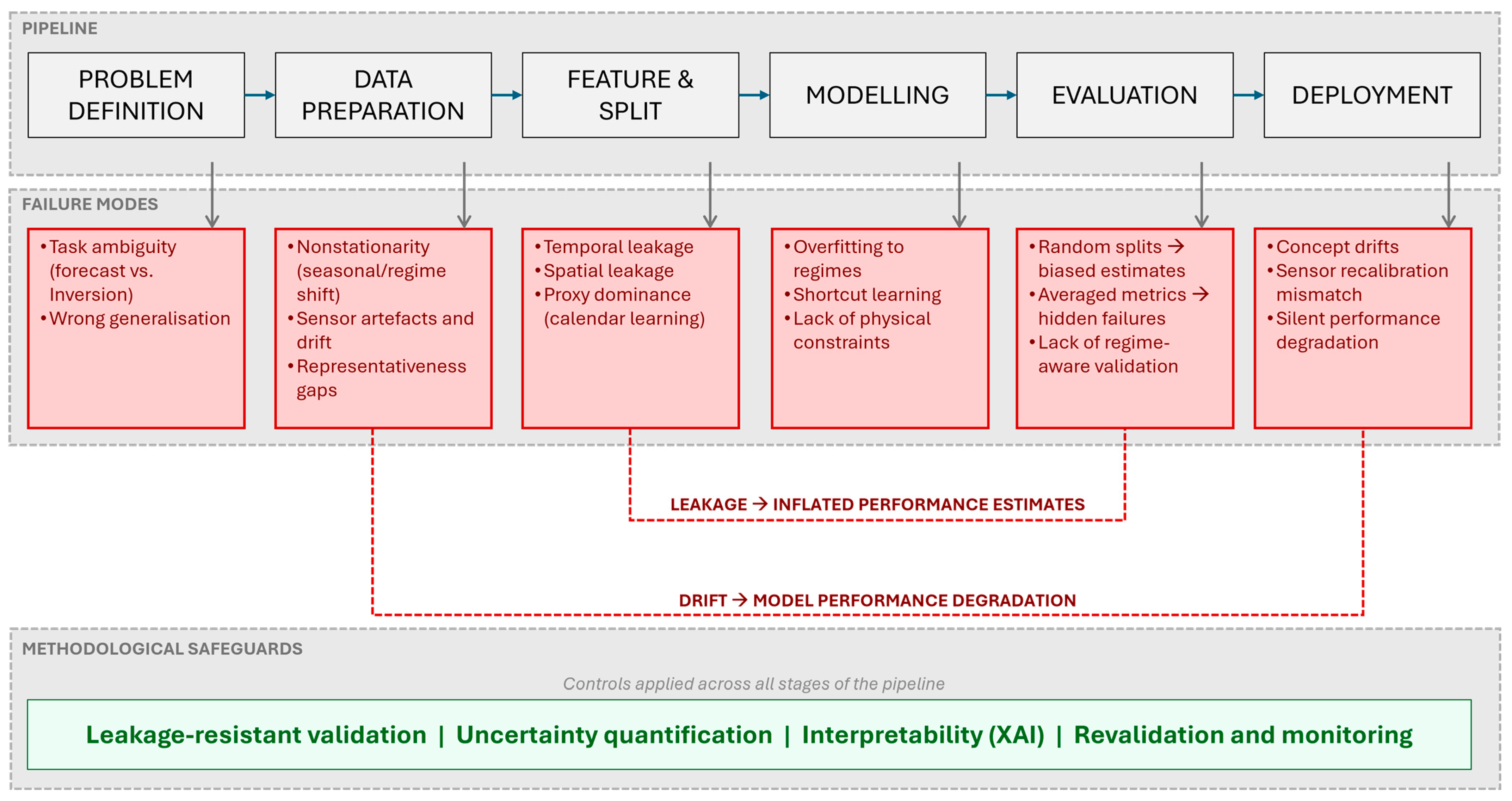
Atmospheric datasets are strongly nonstationary due to seasonality, synoptic variability, regime shifts, and abrupt emission changes; they are also heterogeneous in both measurement characteristics and sampling geometry (stations, satellites, low-cost sensors, model products). Data preparation is therefore not a clerical step but a scientific design choice that shapes what the model can learn and what claims are defensible. These challenges can be systematically interpreted as failure modes arising at different stages of the modelling pipeline, as illustrated in Figure 2.
A robust preparation pipeline begins with representativeness checks: whether training data cover the relevant meteorological and emissions regimes, including extremes. Quality control must be explicit in heterogeneous sensor networks, where spikes, drift, and artefacts can otherwise be mistaken for “signal” [33]. Missingness should be treated as a modelling decision, because the choice of imputation strategy can materially alter performance and uncertainty; sensitivity analysis across imputation methods is therefore recommended [31,32]. For short-term policy or attribution questions, it can also be important to reduce the risk that models succeed primarily by learning calendar regularities (diurnal/weekly/seasonal cycles) rather than event-scale dynamics; refined weather-normalization strategies target this failure mode [34].
Many pipelines also include decomposition-based feature construction. These steps must respect the train/test boundary because applying decomposition to the full dataset before splitting can leak future information into training, inflating apparent skill [35]. When implemented carefully within the training window, decomposition-and-ensemble pipelines can nevertheless help separate temporal components before prediction and improve robustness [36]. Finally, regime discovery and stratification (e.g., clustering by meteorological patterns or pollution regimes) can support balanced training and regime-aware reporting, preventing average scores from hiding systematic failures in stagnation events or transition seasons [21,30,34].

3.3. Validation in Time and Space: Realistic Generalization, Episode Testing, and External Datasets

Because air-quality observations are spatiotemporally dependent, the validation strategy should be chosen according to the scientific claim being made, not treated as a generic technical step. When the goal is prediction over time, blocked-time splits and rolling-origin validation are appropriate because they respect temporal order and prevent future information from leaking into the training window. When prediction across locations is the goal of the modelling, spatial hold-outs (e.g., leave-location-out) are necessary because they test transfer to unseen stations or regions rather than interpolation near sites already represented in training [16,28]. When the goal is robustness under changing emission conditions, evaluation should include held-out periods containing regime shifts, such as lockdowns, policy interventions, or fuel changes, because the relevant question is not only average in-regime accuracy, but performance under nonstationarity and high-impact episodes [30,34]. Treating these validation strategies as interchangeable can lead to misleading conclusions about model performance, particularly in the presence of spatiotemporal dependence and distribution shift.

3.4. Transfer, Domain Shift, and Drift: From “One-Off Accuracy” to Life-Cycle Performance

Even models that validate well can fail under domain shift: changes in emissions, measurement systems, station relocation, meteorological regimes, or chemical environments. Transfer learning and domain adaptation can reuse learned representations for new locations or sensors, but atmospheric deployment requires diagnostics that separate genuine physical change from data artefacts and that quantify how performance degrades under shift [39,45]. Drift is a life-cycle reality for monitoring systems, so operational pipelines should include drift detection triggers, periodic revalidation, and decision rules for recalibration or retraining [45,53,54].
For networked deployments, drift can be heterogeneous (affecting subsets of sensors) and temporally structured (seasonal drift versus abrupt step changes). Monitoring should therefore operate at multiple granularities (site-level, pollutant-level, regime-level) and include quality-control gates and anomaly detection that prevent silent failure propagation into forecasts and decision support [53].

3.5. Uncertainty and Trustworthiness: Probabilistic Outputs, Calibration, and Integrity of Monitoring Pipelines

In operational atmospheric applications, point predictions alone are insufficient; uncertainty estimates should be reported in a form that is both calibrated and physically interpretable. Uncertainty arises from two main sources. The first is inherent atmospheric variability, including turbulent mixing, short-term fluctuations in emissions, and rapidly changing meteorological conditions, which define a natural limit to predictability (aleatoric uncertainty). The second is related to model and data limitations, such as sparse monitoring networks, measurement errors, or distributional shift between training and application conditions (epistemic uncertainty). This distinction is important because it separates uncertainty that cannot be reduced from uncertainty that reflects limitations of the modelling framework [55]. For inverse problems, an additional source of uncertainty is critical. Emission estimates derived from concentration data depend on transport representation, chemical processes, and prior assumptions, and may therefore not be unique. As a result, uncertainty in inferred emissions should be reported explicitly, together with sensitivity to modelling assumptions, rather than represented by a single best estimate [5,6].
For explainable AI to be scientifically useful in atmospheric studies, model explanations must be interpretable in terms of known physical and chemical processes. An explanation is physically meaningful when the attributed predictors correspond to known or mechanistically interpretable drivers of pollutant variability, such as wind speed and direction for dispersion, boundary-layer height for vertical mixing, or stagnation and inversion conditions for pollutant accumulation. By contrast, dominant attribution to shortcut variables such as calendar features, site identifiers, or other non-causal proxies suggests that the model may be exploiting statistical regularities rather than learning atmospheric mechanisms. Practical evaluation should therefore go beyond reporting feature importance alone and include process-based checks, such as predictor ablation, comparison of SHAP-style attributions with known source–meteorology relationships, and testing whether explanations remain consistent with expected differences across pollutants, site types, and seasonal regimes [45].
This idea can be formalized as physically guided feature importance, in which attribution scores obtained from SHAP, LIME, or related XAI methods are systematically evaluated against established domain knowledge rather than interpreted only in statistical terms. The underlying principle is that a model which has genuinely learned the governing physical and chemical processes should produce feature attributions that are consistent, in both sign and relative magnitude, with known regime-dependent directional relationships.
Ozone modelling provides a particularly instructive testbed for this approach. Photochemical ozone formation operates under distinct photochemical regimes: in VOC-limited (NOx-saturated) environments, reducing VOC emissions decreases ozone, whereas reducing NOx may increase it. In NOx-limited environments, the response is reversed. The boundary between these regimes can be characterized empirically through the satellite-derived HCHO/NO2 ratio, which serves as an observational indicator of the relative availability of VOC and NOx precursors, and has been shown to track the transition between regimes across major U.S. urban areas over two decades, providing a chemically grounded benchmark against which model behaviour can be assessed [56]. In a machine learning context, physically guided feature importance requires that the SHAP values assigned to VOC- and NOx-related predictors, radiation, and temperature shift in a regime-consistent manner: VOC-related predictors should dominate attribution in VOC-limited areas, while NOx-related predictors should gain relative importance in NOx-limited regimes. This type of validation has been demonstrated in a LightGBM–SHAP framework applied to ozone formation, where SHAP-derived feature rankings were found to be consistent with TROPOMI-based HCHO/NO2 diagnostics identifying the study area as predominantly VOC-limited, lending credibility to the model’s internal logic beyond what predictive metrics alone could establish [57].
Incorporating physically guided feature importance as a validation step thus strengthens the credibility of XAI outputs in two complementary ways: it provides an independent, domain-grounded check on model behaviour, and it makes explainability results interpretable to domain scientists who may be sceptical of purely data-driven attributions.

4. Applications: Atmospheric Fields and Emission Sources as a Coupled System

Air quality at the surface is an emergent property of a coupled system in which emissions provide time-varying source terms, while meteorology and chemistry control transport, mixing, and transformation of pollutants. In modelling terms, this coupling links (i) the evolution of concentration fields (advection–diffusion–reaction, modulated by boundary-layer dynamics) and (ii) the magnitude and speciation of emissions, which depend on operating conditions and can change rapidly in time. AI methods are increasingly used on both sides of this coupling. On the field side, they support forecasting and spatiotemporal reconstruction of pollutant concentrations from observations, meteorological drivers, and auxiliary products. On the source side, they enable data-driven characterization of emission factors, operating-regime-dependent emission signatures, and sensor-based diagnostics that can act as constraints or inputs for atmospheric applications. The key methodological challenge is ensuring that learned relationships remain valid under regime shifts (meteorological variability, policy-driven emission changes, sensor network evolution) and that evaluation designs reflect intended use without information leakage [1,5,6,16,28].
For clarity, the reviewed studies can be grouped into two main categories: (i) receptor-oriented concentration forecasting and spatiotemporal inference (Section 4.1), and (ii) source-oriented approaches addressing emissions as dynamic source terms (Section 4.2 and Section 4.3). Importantly, only a subset of studies in these categories perform true emission inference in the inverse-problem sense, while many rely on proxy-based modelling of emissions or concentration prediction.

4.1. Atmospheric Pollution Forecasting and Spatiotemporal Inference

Artificial intelligence is now widely used to predict and reconstruct atmospheric pollution fields, including near-surface PM and gas concentrations, across space and time. These applications target both forecasting (e.g., hours to days ahead at stations or grids) and spatiotemporal inference (inferring concentrations at unmonitored locations or producing gridded products from heterogeneous observations). In atmospheric settings, the main difficulty is that pollutant fields reflect a coupled interplay of time-varying emissions, transport, and boundary-layer mixing, and chemical transformation, producing nonstationary behaviour and regime shifts (e.g., stagnation episodes versus advective conditions). Consequently, model design and evaluation must emphasize generalization under changing meteorology/emissions and avoid overly optimistic scores caused by temporal or spatial dependence, which can introduce implicit information leakage when standard random splits are used. Table 1 shows that most approaches focus on concentration prediction using structured spatiotemporal inputs, while relatively fewer studies address emission inference in a physically consistent manner.
Table 1 summarizes representative peer-reviewed studies that illustrate how modern topologies of models address key atmospheric challenges. Most studies in this category focus on concentration prediction and reconstruction, rather than explicit estimation of emissions as source terms. The first atmosphere-facing direction is top-down emission estimation and inventory adjustment for chemical-transport-model (CTM) applications, where neural surrogates of CTM behaviour can enable fast sensitivity analysis and iterative updating of emission inputs while retaining a link to atmospheric physics through the surrogate’s training target and constraints [58]. For station-network forecasting, spatiotemporal graph convolutional networks (ST-GCN) explicitly model inter-station dependencies and provide scalable frameworks for city-level PM prediction [42], including variants with adaptive attention mechanisms that learn dynamic influence patterns across the monitoring network [41]. hybrid deep spatiotemporal models (e.g., CNN–LSTM) remain useful reference points, demonstrating how nonlinear temporal dynamics and spatial coupling can be captured with relatively interpretable components [38]. These architectures are effective because they align with the physical structure of atmospheric processes: temporal models capture persistence and delayed responses driven by transport and boundary-layer evolution, while spatial components represent gradients and inter-station coupling. However, their performance degrades when key drivers of variability (e.g., emissions changes or local meteorology) are not adequately represented in the input data, or when evaluation does not reflect deployment conditions.
The Air Quality Index (AQI) is widely used as an operational, single-value indicator that synthesizes the combined burden of major air pollutants into an interpretable measure of air-quality status and health risk [59,60,61]. In most applications, AQI aggregates information from key criteria pollutants, including PM2.5, PM10, NO2, SO2, CO, and O3, which makes it more useful for communication, warning systems, and policy support than isolated pollutant time series alone [59,60]. At the same time, AQI is not merely a compact reporting metric, because its variability remains strongly shaped by meteorological conditions that govern pollutant accumulation, transport, dispersion, and dilution, including wind speed, rainfall, temperature, and humidity [60,61]. This combination of multi-pollutant aggregation and meteorological sensitivity makes AQI forecasting a particularly demanding spatiotemporal problem: although the target is highly relevant for public-health communication and environmental management, it still reflects nonlinear interactions across pollutants, atmospheric processes, and monitoring locations [59,60,61]. For this reason, AQI provides a natural testbed for graph-based and spatiotemporal deep learning models, which are explicitly designed to learn temporal persistence together with inter-station dependencies that simpler isolated time-series approaches may fail to represent adequately [59].
Alongside architecture choice, several studies emphasize that skill claims are inseparable from evaluation design. Comparative and real-world benchmarking work helps quantify how much improvement is gained over classical baselines and whether gains persist across episodes that matter operationally (alerts, interventions), rather than only in average conditions [29,30]. Importantly, these findings also indicate that reported performance is highly sensitive to validation design, and that realistic evaluation often narrows the gap between model classes.

4.2. Automotive Exhaust Emissions and Toxicity: AI Methods Relevant to Atmospheric Pollution from Mobile Sources

Mobile sources are a major contributor to urban NOx, CO, VOCs and primary particulate matter, and their relevance to population exposure is amplified by strong temporal variability under real driving and by the proximity of emissions to receptors. From an atmospheric-science perspective, the key aim is therefore not engine optimization per se, but the derivation of reliable, time-resolved emission signals and driving-regime-dependent emission factors that can be used to constrain inventories, feed dispersion and exposure models, and support forecasting and scenario analyses [1,2,16].
Recent AI methods contribute to this objective in several complementary ways (Table 2). Virtual sensing approaches learn mappings from on-board operational variables to instantaneous emissions, enabling high-frequency NOx estimation under noisy, nonstationary RDE conditions [62]. Low-latency temporal architectures such as temporal convolutional networks (TCNs) provide transient emission prediction suitable for on-board monitoring as well as for generating high-resolution emission time series that better represent short-lived spikes relevant to near-road impacts [63]. Supervised learning using real-world vehicle activity and road-context data supports dynamic emission modelling that translates kinematics and context into regime-dependent estimates, improving link-level inventories and supporting joint air-quality and climate assessments [64]. At fleet scale, event detection and screening models can identify high-emission episodes or high emitters from remote data streams, enabling targeted mitigation and dynamic inventory correction [65]. In parallel, ML-based models for non-exhaust particulate sources (e.g., brake emissions) help quantify contributions that may dominate urban PM exposure in certain settings and are difficult to capture with traditional exhaust-oriented parameterizations [66].
Finally, unsupervised regime discovery converts raw high-frequency streams into interpretable operating states with distinct emission signatures, supporting regime-conditioned parameterizations and more realistic temporal allocation of emissions [67]. Because mobile emissions are strongly regime-dependent and prone to distribution shift (route, temperature, driver behaviour, vehicle condition), evaluation should reflect intended deployment: time-aware splitting to avoid leakage, robustness checks across operating domains, and reporting of systematic bias in addition to average accuracy [16,28]. This is also evident in Table 2, where studies relying on high-frequency data and sequence-aware models tend to emphasize temporal structure, while approaches based on aggregated or context features may mask short-term variability. In practice, models relying on aggregated or proxy-based inputs may fail to capture short-lived emission spikes and regime transitions, while high-capacity temporal models remain sensitive to data quality, sensor noise, and limited coverage of rare operating conditions.

4.3. Stationary Combustion Diagnostics and Emission-Relevant Modelling: Methods Relevant to Atmospheric Pollution from Point Sources

Stationary combustion systems remain major point sources of NOx, CO and primary particulate emissions, and their emission profiles can change rapidly under load transients, fuel switching, and thermoacoustic instability. From an atmospheric-science perspective, the practical objective is not combustion optimization per se, but extracting time-resolved, regime-aware emission-relevant information that can support point-source characterization, scenario analysis, and (where available) coupling to dispersion/chemistry frameworks as dynamic inputs. In this context, recent AI work contributes in three complementary ways (Table 3): (i) identifying stability boundaries and operational regimes linked to a higher risk of emission excursions, (ii) providing fast instability detection from diagnostic data streams suitable for monitoring and early intervention, and (iii) enabling computational acceleration and sparse-sensing reconstruction that make high-fidelity state information more accessible in practice. Table 3 (continued) includes additional representative studies illustrating emission prediction under different validation strategies.
A first line of work focuses on learning stability maps from operating variables and measured signals to delineate stable versus unstable regimes and to approximate stability limits. Such empirical boundary mapping can be operationally valuable because it translates complex combustor behaviour into actionable “safe operating envelopes,” reducing time spent near unstable conditions that are commonly associated with degraded combustion and higher CO/NOx variability. This is illustrated by neural-network-based stability prediction for industrial gas combustion, where stability regimes are learned directly from operating conditions and measurements and can be used to guide operation toward lower-risk regions [68]. Complementary to boundary mapping, fast instability detection targets the early recognition of thermoacoustic transitions using high-frequency diagnostic streams, where the emphasis is on sensitivity and lead time rather than only average error. Deep spatiotemporal models combining convolutional feature extraction with temporal sequence learning have been demonstrated for rapid detection of combustion instability, supporting online monitoring that can trigger mitigation before high-amplitude oscillations develop and drive short-lived emission spikes [69]. These modern deep learning approaches sit on a longer methodological arc: earlier ANN studies already showed that instability signatures can be learned from measurements, establishing the basic feasibility of data-driven instability prediction and motivating today’s higher-capacity sequence and imaging pipelines [70].
A second direction aligns with the practical reality that industrial systems often operate under limited instrumentation. Here, hybrid digital-twin concepts and sparse-sensing strategies aim to reconstruct emission-relevant states from a small number of sensors while leveraging numerical priors or reduced representations. Adaptive digital twins using sparse sensing have been demonstrated for combustion systems, showing that meaningful state estimation is feasible even when full-field observations are not available, which is directly relevant for translating point-source operation into higher-frequency, better-resolved inputs for atmospheric applications [71]. In parallel, AI-based predictive models for alternative-fuel and dual-fuel operating regimes can support characterization of emission-relevant behaviour under fuel switching (an increasingly common real-world driver of regime change), providing learned mappings between operating conditions and system response that can be used to summarize regime-dependent behaviour and inform scenario-based emission characterization [72]. Finally, chemistry acceleration via deep surrogates enables broader simulation coverage of pollutant-forming pathways that are otherwise computationally prohibitive, which matters when point-source characterization requires richer chemistry (e.g., NH3/H2 combustion with NOx and NH3-slip-relevant pathways). Deep learning chemistry acceleration methods have been proposed to retain acceptable fidelity to detailed kinetics while enabling orders-of-magnitude speed-ups, facilitating more extensive exploration of emission-relevant chemistry in CFD/LES-style analyses [73].
Because point-source behaviour is strongly regime-dependent and can shift with operating mode, load, or fuel, evaluation should reflect intended deployment rather than only retrospective fit. Time-aware splitting helps avoid leakage in high-frequency sequences, robustness checks across operating regimes are necessary to detect failure under transitions [16,28]. In practice, this effect is clearly reflected in comparative modelling studies. Approaches based on random train/test splits often report higher predictive performance, as temporally adjacent observations share similar operating conditions and emission characteristics, leading to implicit information leakage. By contrast, studies explicitly accounting for temporal dependence—including sequence-based models such as LSTM combined with time-aware splitting—typically report lower but more realistic performance, particularly for emission components exhibiting strong transient and regime-dependent behaviour (e.g., CO or OGC). This indicates that the apparent modelling difficulty in combustion-related applications is not solely a property of the model architecture, but emerges from the interaction between data structure, temporal dependence, and validation design [74,75]. Thus, reporting should include systematic bias and failure modes in addition to average metrics. These practices align with established guidance on validation under structured dependence and the known pitfalls of naive cross-validation for time series.
Table 3. Point-source emission estimation and combustion-state diagnostics with AI (stationary sources).
Application/ProblemModel/ArchitectureInput Data and PreprocessingEvaluation Metrics (Typical Reporting)Key Findings (AAS-Relevant Takeaway)Year
Stability boundary mapping for industrial gas burners [69]ANN/MLP classifier–regressor for stability regimes/limitsBurner operating parameters + measured signals; normalization; train/test splitAccuracy/F1 (classification); boundary error; false-alarm rate (where reported)Learns empirical stability maps that support operation within low-risk regimes, reducing probability of unstable combustion associated with CO/NOx excursions2021
Fast instability detection from diagnostic signals (deep sequence classifier) [68]LSTM–CNN hybrid (feature extraction + temporal classification)High-frequency sensor/diagnostic time series (as provided in study); standardization; supervised trainingDetection accuracy/sensitivity; lead time; latency (if reported)Enables early detection of thermoacoustic instability, supporting mitigation before oscillations trigger emission spikes2021
Neural prediction of combustion instability (early ANN approach) [70]Feed-forward ANN/neural predictorExperimental/sensor signals; normalization; supervised trainingPrediction error; classification accuracy (as reported)Early evidence that data-driven predictors can anticipate instability regimes, motivating modern real-time diagnostics for point-source emissions control2002
Sparse-sensing digital twins for industrial combustion monitoring [71]Adaptive digital twin with sparse sensing strategies (hybrid physics–data)Sparse sensor signals + numerical priors; sparse reconstruction/updatingReconstruction error; stability of adaptation; robustness to sensor sparsityDemonstrates feasible monitoring under limited instrumentation, enabling estimation of emission-relevant states in point sources2023
Predictive modelling for H2/NG/Diesel dual-fuel operation (emission-relevant operating regimes) [72] Predictive ML model (as proposed in study)Engine operating variables; preprocessing per study; train/test splitRMSE/MAE/R2 (as reported)Supports mapping of operating regimes for low-carbon fuels; relevant for characterizing point-source emissions under fuel switching scenarios2023
Chemistry acceleration for NH3/H2 combustion (NOx/NH3-slip pathways) [73]DL surrogate for chemical kinetics/closure termsSimulation datasets; state→source mapping; validation vs. detailed chemistrySpeed-up factor; error vs. detailed chemistryReduces cost of detailed chemistry while retaining fidelity, enabling broader inclusion of NOx/NH3-slip-relevant pathways in CFD/LES for point-source characterization2025
Emission prediction under controlled experimental conditions [74]ANN (feed-forward)Heating devices operational parameters, environmental performance of heating devicesRandom train/test splitHigh predictive accuracy, potentially influenced by temporal dependence and leakage effects2024
Time-series emission modelling under dynamic combustion conditions [75]LSTM/sequence-based modelsHeating devices operational parameters, environmental performance of heating devicesTime-aware splittingLower but more realistic performance, highlighting regime dependence and modelling difficulty under temporal variability2025

5. Conclusions and Future Directions: Toward Robust, Physics-Consistent AI for Atmospheric Composition and Emission Sources

This review synthesized recent AI developments for atmospheric pollution through an explicitly process-anchored lens: pollutant concentrations as emergent outcomes of emissions, transport/mixing, chemistry, and removal, with mobile and point sources treated as dynamic source terms rather than static boundary inputs. By separating receptor-side concentration forecasting from source-term inference, we clarified which claims can be supported by predictive models trained on monitoring data and which require inverse-problem structure, physically meaningful priors, and uncertainty-aware coupling to atmospheric models. This framing is aligned with the AAS emphasis on mechanism and interpretability: AI is most scientifically valuable when it strengthens causal reasoning about atmospheric composition, not only when it improves scores.
Across applications, two messages recur. First, the architecture choice must follow data geometry (grids, sequences, networks). It should be justified in terms of the atmospheric dependencies the model is expected to represent (advection-like transport, persistence, regime shifts, extremes). Second, evaluation design is not a technical afterthought, but the backbone of credibility in nonstationary, spatiotemporally dependent systems; leakage-resistant evaluation, regime/episode-aware reporting, and bias diagnostics are essential for trustworthy inference and for operational relevance.
Future work should prioritize robust, physics-consistent hybrid workflows: (i) coupling learned components to dispersion/CTM frameworks for interpretable sensitivity and inversion, (ii) enforcing conservation- and structure-based constraints where feasible, (iii) quantifying uncertainty and calibration under distribution shift, and (iv) developing life-cycle monitoring for drift and sensor artefacts. With these practices, AI can move from “black-box prediction” to a reliable scientific instrument for atmospheric composition—supporting better emission characterization, more defensible forecasts, and clearer links between interventions and observed air-quality outcomes.

Author Contributions

Conceptualization, K.S.-S. and A.K.; methodology, A.K.; validation, K.S.-S. and A.K.; formal analysis, A.K. and K.S.-S.; investigation, K.S.-S. and A.K.; resources, K.S.-S. and A.K.; data curation, K.S.-S. and A.K.; writing—original draft preparation, A.K. and K.S.-S.; writing—review and editing, K.S.-S. and A.K.; visualization, K.S.-S. and A.K.; supervision, K.S.-S.; project administration, K.S.-S. and A.K.; funding acquisition, K.S.-S. All authors have read and agreed to the published version of the manuscript.

Funding

This work was supported by the AGH University of Krakow under grant no. 501.00 210000 10000. The contribution of K.S.-S. was partly supported by the “Excellence Initiative—Research University” programme at the AGH University of Krakow.

Institutional Review Board Statement

Not applicable.

Informed Consent Statement

Not applicable.

Data Availability Statement

This is a review article, and no new datasets were generated by the authors. Relevant data sources are described in the cited original studies.

Conflicts of Interest

Author A.K. is a former employee of MDPI. However, she does not work for the journal Sustainability at the time of submission and publication. The remaining author declares no conflicts of interest.

References

  1. Seinfeld, J.H.; Pandis, S.N. Atmospheric Chemistry and Physics: From Air Pollution to Climate Change, 2nd ed.; John Wiley & Sons: Hoboken, NJ, USA, 2006. [Google Scholar]
  2. Zhang, Y.; Bocquet, M.; Mallet, V.; Seigneur, C.; Baklanov, A. Real-Time Air Quality Forecasting, Part II: State of the Science, Current Research Needs, and Future Prospects. Atmos. Environ. 2012, 60, 656–676. [Google Scholar] [CrossRef] [Scilit]
  3. Yu, M.; Huang, Q.; Li, Z. Deep Learning for Spatiotemporal Forecasting in Earth System Science: A Review. Int. J. Digit. Earth 2024, 17, 2391952. [Google Scholar] [CrossRef] [Scilit]
  4. Reichstein, M.; Camps-Valls, G.; Stevens, B.; Jung, M.; Denzler, J.; Carvalhais, N.; Prabhat. Deep Learning and Process Understanding for Data-Driven Earth System Science. Nature 2019, 566, 195–204. [Google Scholar] [CrossRef] [Scilit]
  5. Enting, I.G. Inverse Problems in Atmospheric Constituent Transport; Cambridge University Press: Cambridge, UK, 2002. [Google Scholar]
  6. Turner, A.J.; Jacob, D.J. Balancing Aggregation and Smoothing Errors in Inverse Models. Atmos. Chem. Phys. 2015, 15, 7039–7048. [Google Scholar] [CrossRef] [Scilit]
  7. Szramowiat-Sala, K.; Styszko, K.; Samek, L.; Kistler, M.; Macherzyński, M.; Ryšavý, J.; Krpec, K.; Horák, J.; Kasper-Giebl, A.; Gołaś, J. Comparative Analysis of Real-Emitted Particulate Matter and PM-Bound Chemicals from Residential and Automotive Sources: A Case Study in Poland. Energies 2023, 16, 6514. [Google Scholar] [CrossRef] [Scilit]
  8. Szramowiat-Sala, K.; Marczak-Grzesik, M.; Karczewski, M.; Kistler, M.; Giebl, A.K.; Styszko, K. Chemical Investigation of Polycyclic Aromatic Hydrocarbon Sources in an Urban Area with Complex Air Quality Challenges. Sci. Rep. 2025, 15, 6987. [Google Scholar] [CrossRef] [Scilit]
  9. Raissi, M.; Perdikaris, P.; Karniadakis, G.E. Physics-Informed Neural Networks: A Deep Learning Framework for Solving Forward and Inverse Problems Involving Nonlinear Partial Differential Equations. J. Comput. Phys. 2019, 378, 686–707. [Google Scholar] [CrossRef] [Scilit]
  10. Karpatne, A.; Atluri, G.; Faghmous, J.H.; Steinbach, M.; Banerjee, A.; Ganguly, A.; Shekhar, S.; Samatova, N.; Kumar, V. Theory-Guided Data Science: A New Paradigm for Scientific Discovery from Data. IEEE Trans. Knowl. Data Eng. 2017, 29, 2318–2331. [Google Scholar] [CrossRef] [Scilit]
  11. Bi, K.; Xie, L.; Zhang, H.; Chen, X.; Gu, X.; Tian, Q. Accurate Medium-Range Global Weather Forecasting with 3D Neural Networks. Nature 2023, 619, 533. [Google Scholar] [CrossRef] [Scilit]
  12. Lam, R.; Sanchez-Gonzalez, A.; Willson, M.; Wirnsberger, P.; Fortunato, M.; Alet, F.; Ravuri, S.; Ewalds, T.; Eaton-Rosen, Z.; Hu, W.; et al. Learning Skillful Medium-Range Global Weather Forecasting. Science 2023, 382, 1416–1421. [Google Scholar] [CrossRef] [Scilit]
  13. Bodnar, C.; Bruinsma, W.P.; Lucic, A.; Stanley, M.; Allen, A.; Brandstetter, J.; Garvan, P.; Riechert, M.; Weyn, J.A.; Dong, H.; et al. A Foundation Model for the Earth System. Nature 2025, 641, 1180–1187. [Google Scholar] [CrossRef] [Scilit]
  14. Gui, K.; Zhang, X.; Che, H.; Li, L.; Zheng, Y.; An, L.; Miao, Y.; Zhao, H.; Dubovik, O.; Holben, B.; et al. Advancing Operational Global Aerosol Forecasting with Machine Learning. Nature 2026, 651, 658–665. [Google Scholar] [CrossRef] [Scilit]
  15. Charafeddine, M.; Brijesh, M.; Krushna, M.; Shobhakar, D. Strategies to Accelerate Climate Risk Management in the Building Sector Using Data-Driven Methods and Tools. Commun. Sustain. 2026, 1, 59. [Google Scholar] [CrossRef] [Scilit]
  16. Roberts David, R.; Volker, B.; Simone, C.; Boyce Mark, S. Cross-Validation Strategies for Data with Temporal, Spatial, Hierarchical, or Phylogenetic Structure. Ecography 2016, 40, 913–939. [Google Scholar] [CrossRef] [Scilit]
  17. Hastie, T.; Tibshirani, R.; Friedman, J. The Elements of Statistical Learning Data Mining, Inference, and Prediction; Springer: Berlin/Heidelberg, Germany, 2008. [Google Scholar]
  18. Friedman, J.H. Greedy Function Approximation: A Gradient Boosting Machine. Ann. Stat. 2001, 29, 1189–1232. [Google Scholar] [CrossRef] [Scilit]
  19. Breiman, L. Random Forests. Mach. Learn. 2001, 45, 5–32. [Google Scholar] [CrossRef] [Scilit]
  20. Cortes, C.; Vapnik, V.; Saitta, L. Support-Vector Networks. Mach. Learn. 1995, 20, 273–297. [Google Scholar] [CrossRef] [Scilit]
  21. Christiansen, B. Atmospheric Circulation Regimes: Can Cluster Analysis Provide the Number? J. Clim. 2007, 20, 2229–2250. [Google Scholar] [CrossRef] [Scilit]
  22. Lecun, Y.; Bengio, Y.; Hinton, G. Deep Learning. Nature 2015, 521, 436–444. [Google Scholar] [CrossRef] [Scilit]
  23. LeCun, Y.; Bottou, L.; Bengio, Y.; Haffner, P. Gradient-Based Learning Applied to Document Recognition. Proc. IEEE 1998, 86, 2278–2323. [Google Scholar] [CrossRef] [Scilit]
  24. Hochreiter, S.; Schmidhuber, J. Long Short-Term Memory. Neural Comput. 1997, 9, 1735–1780. [Google Scholar] [CrossRef] [Scilit] [PubMed]
  25. Cho, K.; Van Merriënboer, B.; Gulcehre, C.; Bahdanau, D.; Bougares, F.; Schwenk, H.; Bengio, Y. Learning Phrase Representations Using RNN Encoder-Decoder for Statistical Machine Translation. In Proceedings of the 2014 Conference on Empirical Methods in Natural Language Processing (EMNLP); Association for Computational Linguistics: Stroudsburg, PA, USA, 2014; pp. 1724–1734. [Google Scholar] [CrossRef] [Scilit]
  26. Vaswani, A.; Brain, G.; Shazeer, N.; Parmar, N.; Uszkoreit, J.; Jones, L.; Gomez, A.N.; Kaiser, Ł.; Polosukhin, I. Attention Is All You Need. In Proceedings of the Advances in Neural Information Processing Systems; Curran Associates, Inc.: Red Hook, NY, USA, 2017; pp. 5998–6008. [Google Scholar]
  27. Kipf, T.N.; Welling, M. Semi-Supervised Classification with Graph Convolutional Networks. In Proceedings of the 5th International Conference on Learning Representations, ICLR 2017, Toulon, France, 24–26 April 2017. [Google Scholar]
  28. Bergmeir, C.; Hyndman, R.J.; Koo, B. A Note on the Validity of Cross-Validation for Evaluating Autoregressive Time Series Prediction. Comput. Stat. Data Anal. 2018, 120, 70–83. [Google Scholar] [CrossRef] [Scilit]
  29. Koçak, E. Comprehensive Evaluation of Machine Learning Models for Real-World Air Quality Prediction and Health Risk Assessment by AirQ+. Earth Sci. Inform. 2025, 18, 447. [Google Scholar] [CrossRef] [Scilit]
  30. Zhang, Z.; Johansson, C.; Engardt, M.; Stafoggia, M.; Ma, X. Improving 3-Day Deterministic Air Pollution Forecasts Using Machine Learning Algorithms. Atmos. Chem. Phys. 2024, 24, 807–851. [Google Scholar] [CrossRef] [Scilit]
  31. Hua, V.; Nguyen, T.; Dao, M.-S.; Nguyen, H.D.; Nguyen, B.T.; Chi Minh City, H. The Impact of Data Imputation on Air Quality Prediction Problem. PLoS ONE 2024, 19, e0306303. [Google Scholar] [CrossRef] [Scilit]
  32. Lee, J.-Y.; Han, S.-H.; Kang, J.-G.; Lee, C.-Y.; Lee, J.-B.; Kim, H.-S.; Yun, H.-Y.; Choi, D.-R.; Lee, J.-Y.; Han, S.-H.; et al. Comparison of Models for Missing Data Imputation in PM-2.5 Measurement Data. Atmosphere 2025, 16, 438. [Google Scholar] [CrossRef] [Scilit]
  33. Zafeirelli, S.; Kavroudakis, D. Comparison of Outlier Detection Approaches in a Smart Cities Sensor Data Context. Int. J. Smart Sens. Intell. Syst. 2024, 17, 20240004. [Google Scholar] [CrossRef] [Scilit]
  34. Dai, Y.; Liu, B.; Tong, C.; Carslaw, D.C.; Mackenzie, A.R.; Shi, Z. Rethinking Machine Learning Weather Normalisation: A Refined Strategy for Short-Term Air Pollution Policies. Atmos. Chem. Phys. 2025, 25, 13585–13596. [Google Scholar] [CrossRef] [Scilit]
  35. Yang, X.; Li, J.; Jiang, X. Research on Information Leakage in Time Series Prediction Based on Empirical Mode Decomposition. Sci. Rep. 2024, 14, 28362. [Google Scholar] [CrossRef] [Scilit] [PubMed]
  36. Maciąg, P.S.; Bembenik, R.; Piekarzewicz, A.; Del Ser, J.; Lobo, J.L.; Kasabov, N.K. Effective Air Pollution Prediction by Combining Time Series Decomposition with Stacking and Bagging Ensembles of Evolving Spiking Neural Networks. Environ. Model. Softw. 2023, 170, 105851. [Google Scholar] [CrossRef] [Scilit]
  37. Jakovljevic, A.; Charlin, L.; Barbeau, B. Applying Recurrent Neural Networks and Blocked Cross-Validation to Model Conventional Drinking Water Treatment Processes. Water 2024, 16, 1042. [Google Scholar] [CrossRef] [Scilit]
  38. Tsokov, S.; Lazarova, M.; Aleksieva-Petrova, A.; Tsokov, S.; Lazarova, M.; Aleksieva-Petrova, A. A Hybrid Spatiotemporal Deep Model Based on CNN and LSTM for Air Pollution Prediction. Sustainability 2022, 14, 5104. [Google Scholar] [CrossRef] [Scilit]
  39. Ma, J.; Li, Z.; Cheng, J.C.P.; Ding, Y.; Lin, C.; Xu, Z. Air Quality Prediction at New Stations Using Spatially Transferred Bi-Directional Long Short-Term Memory Network. Sci. Total Environ. 2020, 705, 135771. [Google Scholar] [CrossRef] [Scilit] [PubMed]
  40. Wang, C.; Zhu, Y.; Zang, T.; Liu, H.; Yu, J. Modeling Inter-Station Relationships with Attentive Temporal Graph Convolutional Network for Air Quality Prediction. In Proceedings of the 14th ACM International Conference on Web Search and Data Mining, WSDM 2021, Virtual, 8–12 March 2021; pp. 616–624. [Google Scholar] [CrossRef] [Scilit]
  41. Liu, H.; Han, Q.; Sun, H.; Sheng, J.; Yang, Z. Spatiotemporal Adaptive Attention Graph Convolution Network for City-Level Air Quality Prediction. Sci. Rep. 2023, 13, 13335. [Google Scholar] [CrossRef] [Scilit]
  42. Ni, Q.; Wang, Y.; Yuan, J. Adaptive Scalable Spatio-Temporal Graph Convolutional Network for PM2.5 Prediction. Eng. Appl. Artif. Intell. 2023, 126, 107080. [Google Scholar] [CrossRef] [Scilit]
  43. Heidari, P.; Milan, A. Combining K-Fold Cross Validation with Bayesian Hyperparameter Optimization for Accuracy Enhancement of Land Cover and Land Use Classification. Sci. Rep. 2025, 15, 39758. [Google Scholar] [CrossRef] [Scilit]
  44. Ahmed, M.; Kong, J.; Jiang, N.; Duc, H.N.; Puppala, P.; Azzi, M.; Riley, M.; Barthelemy, X.; Ahmed, M.; Kong, J.; et al. A Bayesian-Optimized Surrogate Model Integrating Deep Learning Algorithms for Correcting PurpleAir Sensor Measurements. Atmosphere 2024, 15, 1535. [Google Scholar] [CrossRef] [Scilit]
  45. Flora, M.L.; Potvin, C.K.; McGovern, A.; Handler, S. A Machine Learning Explainability Tutorial for Atmospheric Sciences. Artif. Intell. Earth Syst. 2024, 3, e230018. [Google Scholar] [CrossRef] [Scilit]
  46. Bai, S.; Kolter, J.Z.; Koltun, V. An Empirical Evaluation of Generic Convolutional and Recurrent Networks for Sequence Modeling. arXiv 2018, arXiv:1803.01271. [Google Scholar] [CrossRef] [Scilit]
  47. Tian, X.; Zhang, C.; Liu, H.; Zhang, B.; Lu, C.; Jiao, P.; Ren, S. Research on Air Quality in Response to Meteorological Factors Based on the Informer Model. Sustainability 2024, 16, 6794. [Google Scholar] [CrossRef] [Scilit]
  48. Gilmer, J.; Schoenholz, S.S.; Riley, P.F.; Vinyals, O.; Dahl, G.E. Neural Message Passing for Quantum Chemistry. In Proceedings of the 34th International Conference on Machine Learning; PMLR: Sydney, Australia, 2017. [Google Scholar]
  49. Tarantola, A. Inverse Problem Theory and Methods for Model Parameter Estimation; Society for Industrial and Applied Mathematics: Philadelphia, PA, USA, 2005. [Google Scholar]
  50. Eugenia, K. Atmospheric Modeling, Data Assimilation and Predictability; Cambridge University Press: Cambridge, UK, 2003. [Google Scholar]
  51. Rodgers, C.D. Inverse Methods for Atmospheres: Theory and Practice; World Scientific Publishing: Singapore, 2000; Volume 2. [Google Scholar]
  52. Evensen, G. The Ensemble Kalman Filter: Theoretical Formulation and Practical Implementation. Ocean Dyn. 2003, 53, 343–367. [Google Scholar] [CrossRef] [Scilit]
  53. Galaz, V.; Centeno, M.A.; Callahan, P.W.; Causevic, A.; Patterson, T.; Brass, I.; Baum, S.; Farber, D.; Fischer, J.; Garcia, D.; et al. Artificial Intelligence, Systemic Risks, and Sustainability. Technol. Soc. 2021, 67, 101741. [Google Scholar] [CrossRef] [Scilit]
  54. Gama, J.; Žliobaitė, I.; Bifet, A.; Pechenizkiy, M.; Bouchachia, A. A Survey on Concept Drift Adaptation. ACM Comput. Surv. (CSUR) 2014, 46, 1–37. [Google Scholar] [CrossRef] [Scilit] [PubMed]
  55. Irrgang, C.; Boers, N.; Sonnewald, M.; Barnes, E.A.; Kadow, C.; Staneva, J.; Saynisch-Wagner, J. Towards Neural Earth System Modelling by Integrating Artificial Intelligence in Earth System Science. Nat. Mach. Intell. 2021, 3, 667–674. [Google Scholar] [CrossRef] [Scilit]
  56. Jin, X.; Fiore, A.; Boersma, K.F.; Smedt, I.D.; Valin, L. Inferring Changes in Summertime Surface Ozone–NOx–VOC Chemistry over U.S. Urban Areas from Two Decades of Satellite and Ground-Based Observations. Environ. Sci. Technol. 2020, 54, 6518–6529. [Google Scholar] [CrossRef] [Scilit]
  57. Yao, T.; Lu, S.; Wang, Y.; Li, X.; Ye, H.; Duan, Y.; Fu, Q.; Li, J. Revealing the Drivers of Surface Ozone Pollution by Explainable Machine Learning and Satellite Observations in Hangzhou Bay, China. J. Clean. Prod. 2024, 440, 140938. [Google Scholar] [CrossRef] [Scilit]
  58. Huang, L.; Liu, S.; Yang, Z.; Xing, J.; Zhang, J.; Bian, J.; Li, S.; Sahu, S.K.; Wang, S.; Liu, T.Y. Exploring Deep Learning for Air Pollutant Emission Estimation. Geosci. Model Dev. 2021, 14, 4641–4654. [Google Scholar] [CrossRef] [Scilit]
  59. Cui, S.; Yang, Y.; Liu, G.; Shen, L. Air Quality Index Prediction Based on Spatio-Temporal Graph Neural Networks: An Empirical Study of Xi’an, China. Eng. Appl. Artif. Intell. 2026, 166, 113547. [Google Scholar] [CrossRef] [Scilit]
  60. Ali, D.; Singh, M.; Khan, A.A.; Vidyarthi, A.K.; Ahmed, S. Impact of Meteorological Drivers on Air Quality Index: A Case Study from Delhi. Environ. Pollut. 2026, 388, 127324. [Google Scholar] [CrossRef] [Scilit]
  61. Wu, Y.; Jin, G.; Li, X.; Huang, H.; Sheng, Z.; Liao, Q. A Novel IDBO-VMD-ITransformer Framework for Air Quality Index Prediction: Multi-Strategy Optimization and Environmental Sustainability Assessment. Process Saf. Environ. Prot. 2026, 207, 108379. [Google Scholar] [CrossRef] [Scilit]
  62. Li, J.; Yu, Y.; Wang, Y.; Zhao, L.; He, C.; Li, J.; Yu, Y.; Wang, Y.; Zhao, L.; He, C. Prediction of Transient NOx Emission from Diesel Vehicles Based on Deep-Learning Differentiation Model with Double Noise Reduction. Atmosphere 2021, 12, 1702. [Google Scholar] [CrossRef] [Scilit]
  63. Liao, J.; Hu, J.; Chen, P.; Zhu, L.; Wu, Y.; Cai, Z.; Wu, H.; Wang, M. Prediction of the Transient Emission Characteristics from Diesel Engine Using Temporal Convolutional Networks. Eng. Appl. Artif. Intell. 2024, 127, 107227. [Google Scholar] [CrossRef] [Scilit]
  64. Li, S.; Tong, Z.; Haroon, M. Estimation of Transport CO2 Emissions Using Machine Learning Algorithm. Transp. Res. D Transp. Environ. 2024, 133, 104276. [Google Scholar] [CrossRef] [Scilit]
  65. Ge, Y.; Hou, P.; Lyu, T.; Lai, Y.; Su, S.; Luo, W.; He, M.; Xiao, L. Machine Learning-Aided Remote Monitoring of NOx Emissions from Heavy-Duty Diesel Vehicles Based on OBD Data Streams. Atmosphere 2023, 14, 651. [Google Scholar] [CrossRef] [Scilit]
  66. Wei, N.; Men, Z.; Ren, C.; Jia, Z.; Zhang, Y.; Jin, J.; Chang, J.; Lv, Z.; Guo, D.; Yang, Z.; et al. Applying Machine Learning to Construct Braking Emission Model for Real-World Road Driving. Environ. Int. 2022, 166, 160–4120. [Google Scholar] [CrossRef] [Scilit]
  67. Mehnatkesh, H.; Gordon, D.; Koch, C.R. Dynamic Emission Analysis of a Hydrogen/Diesel Dual-Fuel Engine Using Clustering Method. Int. J. Hydrogen Energy 2025, 136, 371–382. [Google Scholar] [CrossRef] [Scilit]
  68. Lyu, Z.; Jia, X.; Yang, Y.; Hu, K.; Zhang, F.; Wang, G.; Lyu, Z.; Jia, X.; Yang, Y.; Hu, K.; et al. A Comprehensive Investigation of LSTM-CNN Deep Learning Model for Fast Detection of Combustion Instability. Fuel 2021, 303, 121300. [Google Scholar] [CrossRef] [Scilit]
  69. Zhang, L.; Xue, Y.; Xie, Q.; Ren, Z. Analysis and Neural Network Prediction of Combustion Stability for Industrial Gases. Fuel 2021, 287, 119507. [Google Scholar] [CrossRef] [Scilit]
  70. Cammarata, L.; Fichera, A.; Pagano, A. Neural Prediction of Combustion Instability. Appl. Energy 2002, 72, 513–528. [Google Scholar] [CrossRef] [Scilit]
  71. Procacci, A.; Amaduzzi, R.; Coussement, A.; Parente, A. Adaptive Digital Twins of Combustion Systems Using Sparse Sensing Strategies. Proc. Combust. Inst. 2023, 39, 4257–4266. [Google Scholar] [CrossRef] [Scilit]
  72. Sehili, Y.; Loubar, K.; Tarabet, L.; Cerdoun, M.; Lacroix, C. Development of Predictive Model for Hydrogen-Natural Gas/Diesel Dual Fuel Engine. Energies 2023, 16, 6943. [Google Scholar] [CrossRef] [Scilit]
  73. Wu, S.; Liang, W.; Luo, K.H. Deep Learning Based Combustion Chemistry Acceleration Method for Widely Applicable NH3/H2 Turbulent Combustion Simulations. Combust. Flame 2025, 278, 114218. [Google Scholar] [CrossRef] [Scilit]
  74. Szramowiat-Sala, K.; Penkala, R.; Horák, J.; Krpec, K.; Hopan, F.; Ryšavý, J.; Borovec, K.; Górecki, J. AI-Based Data Mining Approach to Control the Environmental Impact of Conventional Energy Technologies. J. Clean. Prod. 2024, 472, 143473. [Google Scholar] [CrossRef] [Scilit]
  75. Szramowiat-Sala, K.; Krpec, K.; Penkala, R.; Ryšavý, J. Data-Driven Prediction of Pollutants Emission from Small-Scale Heating Units Using Temporal Deep Learning. Energy Convers. Manag. X 2025, 28, 101322. [Google Scholar] [CrossRef] [Scilit]
Figure 1. Conceptual framework for AI-based atmospheric modelling (source: own preparation).
Sustainability 18 04838 g001
Figure 2. Failure-aware workflow for AI-based atmospheric modelling under nonstationary and spatiotemporally dependent conditions (source: own preparation).
Sustainability 18 04838 g002
Table 1. Representative AI applications for atmospheric pollution forecasting and spatiotemporal inference.
Application/ProblemModel/ArchitectureInput Data and PreprocessingEvaluation MetricsKey FindingsYear
Emission inventory estimation/top-down correction for CTM applications [58]NN-CTM (neural-network surrogate of a comprehensive CTM) + gradient-based emission updatingCTM simulations + surface monitoring constraints; surrogate training + iterative emission adjustmentSurrogate similarity vs. CTM; concentration error reduction (MAE/RMSE as reported); emission incrementsDemonstrates that a NN surrogate can emulate CTM behaviour and support inventory updating that improves agreement with observations—directly relevant for building better emission inputs for atmospheric modelling2021
City-scale PM2.5 prediction (scalable graph learning) [42]Adaptive scalable spatio-temporal graph convolutional network (ST-GCN)Station-network time series; graph construction; scaling/normalizationRMSE/MAE/R2 (as reported)Captures space–time dependencies across monitoring networks and scales to larger city deployments, supporting operational forecasting2023
City-level air-quality prediction (adaptive attention on graphs) [41]Spatiotemporal adaptive attention graph convolution networkMulti-station time series; adaptive graph attention; standard preprocessingRMSE/MAE/R2 (as reported)Learns dynamic inter-station influence patterns, improving city-level predictions in heterogeneous monitoring networks2023
Hybrid deep spatiotemporal forecasting [38]CNN–LSTM hybrid spatiotemporal modelHistorical pollutant time series + spatiotemporal features; scaling; train/val/test splitRMSE/MAE/R2 (as reported)Illustrates a strong “classic” deep baseline for capturing nonlinear dynamics and space–time coupling in air-pollution forecasting2022
Deterministic air-pollution forecast improvement (3-day) [30]ML post-processing/algorithm comparison for forecast correctionMonitoring + meteorological predictors (and/or model outputs, per setup); standard preprocessingRMSE/MAE, bias/skill (as reported)Shows that ML correction layers can improve short-range deterministic forecasts and reduce systematic error2024
Real-world AQ prediction + health risk assessment [29]Comprehensive ML evaluation suite (model benchmarking)Air-quality time series; model-specific preprocessing (as reported)Forecast errors (RMSE/MAE/R2) + task-specific metrics (as reported)Provides a structured benchmark illustrating how model choice impacts predictive skill under real-world conditions, useful as a reference baseline2025
Table 2. Mobile-source emission modelling with AI: virtual sensing, transient prediction and fleet-scale screening.
Application/ProblemModel/ArchitectureInput Data and PreprocessingEvaluation MetricsKey FindingsYear
Virtual NOx sensing under real driving conditions (RDE) [62]Signal decomposition + sequence learning (e.g., SSA/ICEEMDAN + GRU) with regression (e.g., SVR)On-road time series (engine/aftertreatment/vehicle signals); denoising + decomposition; component selection; normalizationRMSE, MAE, R2 (often segment-/route-wise)Enables high-frequency NOx estimation from operational signals, supporting time-resolved emission profiles for near-road air-quality and exposure applications2021
Low-latency transient emission prediction for on-board monitoring [63]Temporal convolutional network (TCN; dilated causal conv + residual blocks)Driving-cycle sequences (e.g., WHTC/RDE segments); scaling; train/validation/test splitsRMSE/MAE/R2; inference latency (where reported)Provides fast transient emission predictions suitable for real-time monitoring and generation of high-resolution emission time series2024
Dynamic emission modelling from real-world vehicle activity data (CO2) [64]Supervised ML (e.g., gradient boosting or LSTM-based sequence models)PEMS + GPS/road context; kinematic features (speed/acceleration/grade), VSP; filtering; normalizationRMSE/R2; bias across road types/driving regimesDerives driving-regime-dependent emission factors from real-world data, improving link-level inventories and supporting coupled air-quality–climate assessments2023–2024
Fleet-scale detection of high-emission events (high-NOx/high emitters) [65]ML classification/early-warning (e.g., random forest or related ensembles)Remote OBD/telematics streams + operating context; feature engineering; imbalance handlingClassification metrics (F1/AUROC), detection rate/false alarmsIdentifies high-emission episodes/vehicles at scale, enabling targeted mitigation and dynamic inventory corrections for urban modelling2023
Non-exhaust PM source modelling under real-world driving (brake emissions) [66]Data-driven emission model (ML regression with context features)Driving kinematics + braking intensity/context + measured non-exhaust PM; preprocessing aligned to measurement protocolPrediction error vs. baseline; scenario sensitivityQuantifies non-exhaust PM contributions that can dominate urban particulate exposure in specific settings, improving source representation2022
Emission regime discovery and state identification from high-frequency streams [67]Unsupervised clustering + regime statistics (e.g., k-means/state identification)Instantaneous emissions + driving/engine states; scaling; validity checksCluster validity indices; regime-wise emission deltasConverts raw RDE/PEMS streams into interpretable operating regimes with distinct emission signatures, supporting regime-conditioned parameterizations2025
Disclaimer/Publisher’s Note: The statements, opinions and data contained in all publications are solely those of the individual author(s) and contributor(s) and not of MDPI and/or the editor(s). MDPI and/or the editor(s) disclaim responsibility for any injury to people or property resulting from any ideas, methods, instructions or products referred to in the content.