Predicting Public Transit Demand Using Urban Imagery with a Dual-Latent Deep Learning Framework

Abstract

Public transit demand forecasting is a foundational component of sustainable urban mobility, enabling efficient operation, equitable service provision, and planning of public transit systems. Urban imagery, such as aerial images, contains rich information about urban sociodemographic characteristics and the built environment, offering particular value for data-scarce regions where conventional datasets are limited or outdated. However, there is limited research on using these images for public transit demand forecasting. This study introduces a deep learning approach for predicting transit ridership using aerial images. The method employs an encoder–decoder architecture to functionally separate image-derived latent representations into sociodemographic and physical environment vectors, which are subsequently used as inputs to a neural network for ridership prediction. Using data from Seoul, South Korea, the effectiveness of the proposed method is evaluated against three baseline configurations. The results show that the sociodemographic latent vector captures spatially organized residential characteristics, while the physical environment vector encodes distinct urban landscape patterns such as dense housing, traditional street grids, open spaces, and natural environments. The proposed model, which uses only imagery-derived latent features, substantially outperforms the pure image baseline and narrows the performance gap with census-informed models, reducing sMAPE by 25–60% depending on the mode. Combining imagery with census variables yields the highest accuracy, confirming their complementary nature. These findings highlight the potential of imagery-based approaches as a scalable, cost-efficient, and sustainable tool for data-driven transit planning.

1. Introduction

Many cities around the world are striving to advance sustainable and low-carbon transportation systems by encouraging the use of public transit. To support these goals, accurately predicting public transit demand is essential for ensuring efficient operations, equitable service provision, and environmentally responsible mobility planning [1,2]. In these demand prediction models, sociodemographic indicators and the features of the built environment are significant variables [3,4,5,6,7], which are traditionally collected and utilized in numerical form through field surveys and questionnaires. However, these datasets are often costly to obtain, infrequently updated, and in many regions unavailable, posing challenges for sustainable and data-driven transit planning.

Recent advancements in deep learning have revealed that urban imagery, including aerial imagery and satellite imagery, contains diverse information about urban areas, such as sociodemographic factors, built environment characteristics, land cover, and urban form [8]. Images can be used to estimate the population, economic status, and commercial activity, thus assessing the sociodemographic conditions of cities. Additionally, features extracted from these images can facilitate land cover monitoring and the identification of urban elements such as buildings, vehicles, and ships. If urban imagery can indeed provide information about a city’s sociodemographic conditions and urban environment, it stands to reason that image-based public transit demand prediction might also be feasible.

Despite the promising potential of urban imagery, current research on its application in the transportation sector is still limited. Existing studies have focused mainly on numerical data for predicting public transit demand, overlooking the rich, high-dimensional information available in urban imagery. As a result, the potential of imagery for transportation planning, particularly for supporting sustainable and equitable public transit systems, has not yet been fully explored. To bridge this gap, this study proposes a novel image-based framework for predicting public transit demand without requiring direct access to observed sociodemographic data. The key idea is to decompose urban imagery into two complementary latent spaces: a sociodemographic latent vector learned by predicting demographic attributes from images, and a physical environment latent vector that captures the remaining visual information. These representations are learned through a sequential, knowledge-guided training strategy that functionally separates demographic and physical features, enabling more interpretable and transferable image-based demand prediction. By integrating these disentangled latent vectors into a transit demand prediction network, this study introduces a new way to leverage imagery for transportation analysis that is scalable, interpretable, and data-efficient.

2. Literature Review

2.1. Public Transit Demand

The conventional approach for public transit demand modeling is conducted using the “four-step” demand estimation model. While the four-step model may be suitable for macroscopic analyses at the administrative district level, its accuracy and ability to predict usage patterns are limited in densely populated areas. To complement the four-step demand model, the Direct Ridership Model (DRM) can be utilized. The DRM directly predicts transit ridership based on the built environment, land use characteristics, transit service features, and the sociodemographic attributes of passengers. This method is time-efficient, reduces labor costs, and offers interpretability by revealing the relationship between station ridership and surrounding land use characteristics. The most used method for station-level passenger modeling in DRM is multiple regression analysis [9]. To account for spatial heterogeneity, Geographically Weighted Regression (GWR) is also widely employed [10,11]. Additionally, artificial intelligence methodologies, such as Random Forest [12] and Gradient Boosting Regression Tree Models [13], are frequently used to capture nonlinear relationships with ridership.

In the Direct Ridership Model, the primary variables that significantly impact ridership are sociodemographic and built environment variables. Ridership tends to be higher in areas with high population and employment densities [14,15,16]. Certain sociodemographic groups also play an important role. For instance, areas with a larger proportion of youth tend to exhibit higher ridership, while areas with a greater share of elderly or high-income residents generally show lower transit use [17,18]. In addition, transit usage is related to urban structure and the built environment, with higher usage tendencies in urban centers and areas with mixed land use [7,19,20,21]. Factors such as the ratio of green spaces and the ratio between buildings are also crucial determinants of transit usage [20,22]. Although a variety of socio-structural and built environment variables influence ridership, practical constraints such as modeling algorithms, computational power, and data collection costs have limited most models to using fewer than a certain number of variables. Additionally, to the best of our knowledge, most studies have relied on structured data, and there is no existing research that models ridership using urban imagery to capture the actual urban landscape.

2.2. Urban Imagery

Urban imagery provides a depiction of the Earth’s surface, offering comprehensive information about urban environments, forms, and sociodemographic characteristics. First, lower-level information about the urban environment can be obtained, such as the amount of vegetation, the area of the building, and the geometry. In addition, it has been shown to include higher-level information on land use classification [23,24,25] and is well-suited to understanding urban form and context [26,27]. Furthermore, recent deep-learning research has shown that urban imagery can be used to infer sociodemographic information. It enables the identification of characteristics of the urban population, inference of economic status, and mapping of poverty [28,29,30]. Early studies on predicting sociodemographic indicators were conducted on a macroscopic scale of 25 km × 25 km [23], but recent studies have demonstrated that predictions can also be made on a more granular scale [28].

Individual pixels in urban imagery do not inherently carry meaningful information. To extract significant insights from urban imagery, various modeling approaches can be employed. First, domain-specific knowledge can be used to aggregate pixel-level attributes for modeling. For example, studies have shown that increases in nighttime lights are strong predictors of national economic growth [31], and urban vegetation indices are related to heat-related mortality [32]. Second, convolutional neural networks (CNNs) can be utilized to estimate various indicators such as population, economic livelihood, and land use [26,33]. Third, transfer learning can be applied by training a model on a large, labeled dataset and then fine-tuning it for the specific target of interest. Ayush et al. [30] demonstrated this approach by using high-resolution images to detect buildings, vehicles, and objects, thereby accurately estimating economic well-being in Uganda. Fourth, generative models can be used to effectively compress image vectors and learn good representations, leading to strong performance. For instance, Fu et al. [34] proposed a convolutional autoencoder model to extract important features to predict minute-level solar photovoltaic power.

Based on the literature review, it was identified that the use of urban imagery for public transit demand analysis is better aligned with Direct Ridership Modeling than with the traditional “four-step” modeling framework. This is because it is possible to infer sociodemographic indicators and understand the physical environment even at a micro-level. To enhance prediction accuracy, it is essential that relevant information be effectively extracted from images, including sociodemographic attributes and built-environment features. Accordingly, an encoder–decoder–based model is employed to extract attributes related to both sociodemographic indicators and the urban environment.

3. Methodology

3.1. Problem Definition

The primary objective of this study is to predict public transit demand at the grid-cell level using urban imagery. Let ${\mathbf{x}}_i\in {\mathbb{R}}^{H\times W\times C}$ denote an aerial image corresponding to grid cell i, where C represents the number of color channels (e.g., Red, Green and Blue), and $H\times W$ denotes the spatial dimensions (height and width). Each grid cell also has a corresponding value of sociodemographic indicators and public transit demand values: a vector of sociodemographic indicators ${\mathbf{d}}_i\in {\mathbb{R}}^f$, and a vector of public transit demand values ${\mathbf{y}}_i\in {\mathbb{R}}^m$.

This paper proposes a model that utilizes urban imagery to predict public transit demand. The primary objective of the proposed model in this study is to predict public transit demand using urban imagery. Public transit demand is estimated by predicting the average weekday ridership for both subways and buses, including boarding, alighting, and total passenger counts. We also aimed to consider public bikes, which are a widely used public mode nowadays. The model considers variables that influence public transit usage, specifically sociodemographic indicators and the built environment, which are derived from aerial imagery.

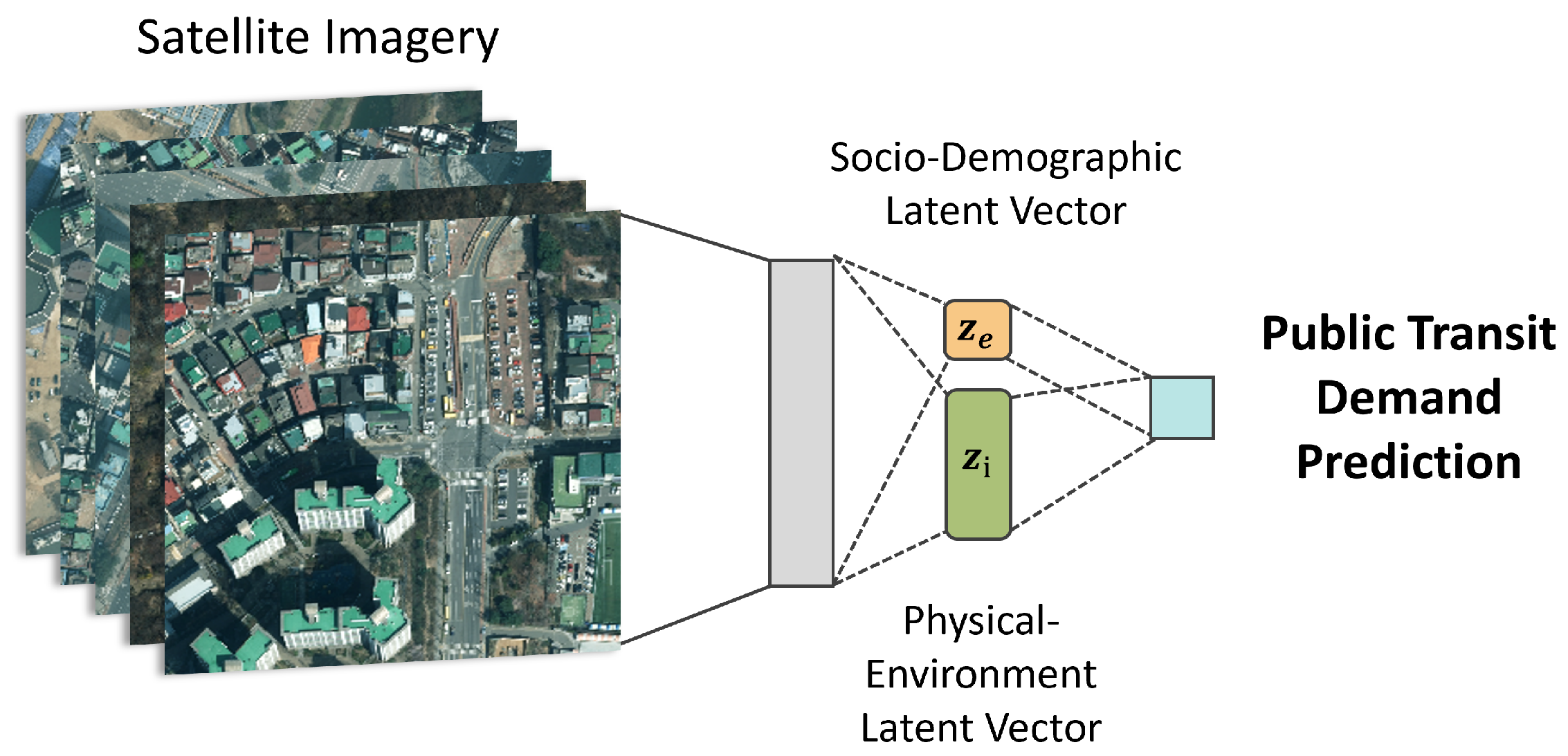
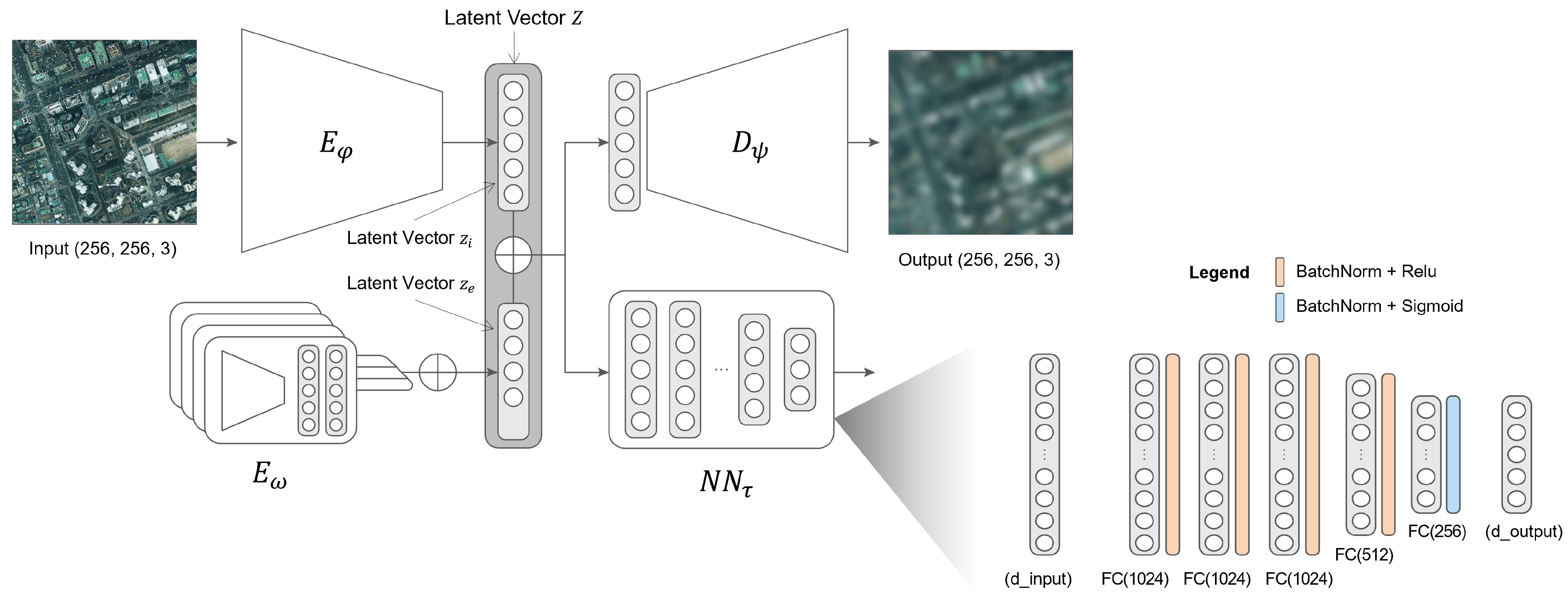
As shown in Figure 1, the core idea of the model is to use urban imagery as input and extract two latent vectors: a sociodemographic vector $z_e$ and a physical environment vector $z_i$. These two vectors are jointly used to predict public transit demand at the spatial grid level. The sociodemographic vector $z_e$ includes variables such as gender, age distribution, household characteristics, and other relevant factors. The physical environment latent vector $z_i$ captures complementary features from the urban imagery that are not explicitly contained in $z_e$. These two vectors are designed to be disjoint so that $z_i$ focuses on image-derived features orthogonal to the sociodemographic information in $z_e$.

3.2. Approach/Methodology

This section describes the framework of the public transit ridership prediction model. The model integrates sociodemographic information and image-based representations by learning two functionally specialized latent vectors: a sociodemographic latent vector $z_e$ and the physical environment latent vector $z_i$. The objective is to predict transit ridership demand from these latent representations. The model adopts an encoder–decoder structure, taking images as input and reconstructing them during training. The compressed latent vectors from the image information consist of $z_e$ and $z_i$. The network comprises $E_{\omega }$ for learning $z_e$, $E_{\phi }$ and $D_{\psi }$ for learning $z_i$, and $N{N}_{\tau }$ for predicting public transit demand using vectors $z_e$ and $z_i$.

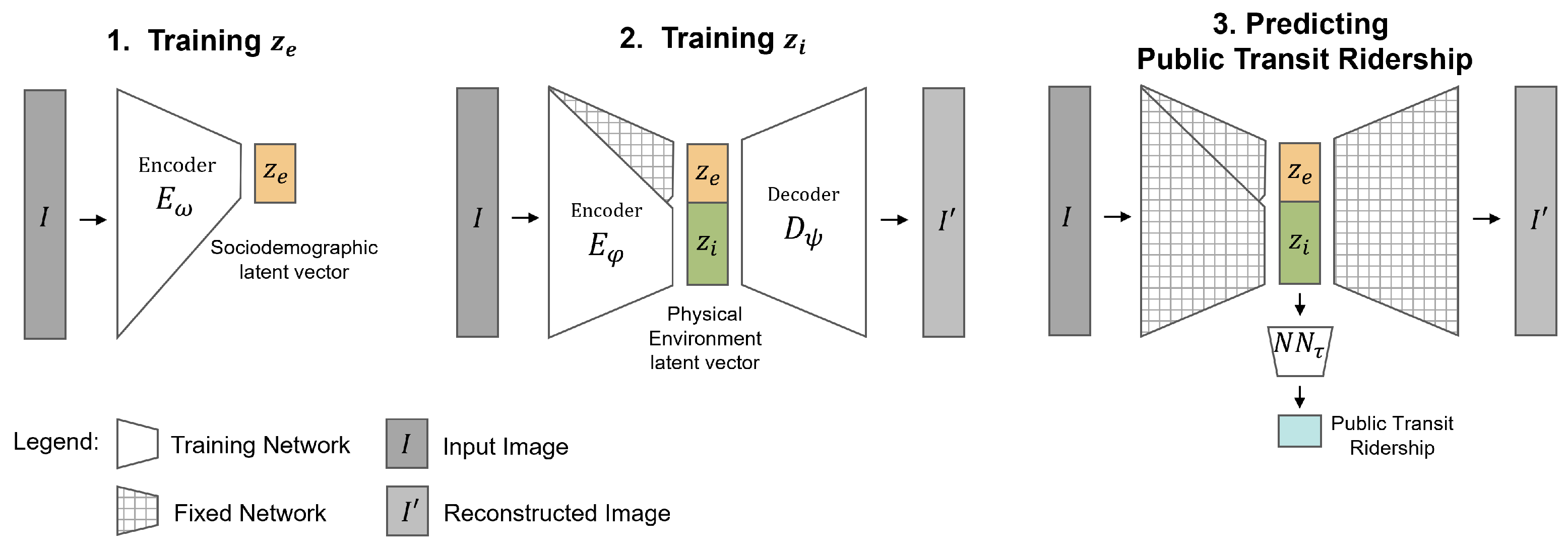
As shown in Figure 2, the model follows a three-stage sequential training strategy. First, the network $E_{\omega }$ is trained to estimate the sociodemographic vector $z_e$ from the input image. Second, with $E_{\omega }$ fixed, the learned $z_e$ is incorporated into an auto-encoder framework to reconstruct the input image. In this stage, the encoder $E_{\phi }$ and decoder $D_{\psi }$ are trained to learn the complementary latent vector $z_i$, which captures the remaining visual information not represented in $z_e$. This design assumes that physical environment characteristics are encoded in the latent vector $z_i$. Although the framework does not explicitly impose orthogonality or independence between $z_e$ and $z_i$, the distinct training objectives guide a functional separation informed by the different training objectives.

Finally, a model $N{N}_{\tau }$ is trained to predict travel demand using the concatenated vector of the two latent vectors, $z_e$ and $z_i$, as input. Although the final prediction network receives the fused latent representation $z_e$ and $z_i$, the model is not trained as an end-to-end fused network. Instead, the architecture adopts a late-fusion approach, where the two latent vectors are first learned independently and subsequently combined only during the prediction stage. This sequential design ensures that $z_e$ captures sociodemographic attributes, while $z_i$ encodes the remaining physical information extracted from the image.

3.2.1. Training $z_e$, the Sociodemographic Latent Vector

The encoder network receives an image as input and estimates a sociodemographic latent vector $z_e$ that encodes attributes such as population, household composition, and employment structure. Each element $z_{e,j}$ of this vector corresponds to one sociodemographic attribute, and the encoder learns to minimize the difference between each true value $z_{e,j}$ and its predicted counterpart ${\widehat{z}}_{e,j}$.

For attributes represented as probability distributions, the encoder maximizes the likelihood of the observed data. This process is equivalent to minimizing the Kullback–Leibler (KL) divergence, as shown in Equation (1). The explicit form of this divergence is provided in Equation (2).

$$arg\underset{\omega }{min}{D}_{\mathrm{KL}}(p\left(z_{e,j}\right)\Vert { q}_{\omega }\left({\widehat{z}}_{e,j}\right))$$

(1)

$$D_{\mathrm{KL}}(p\left(z_{e,j}\right)\Vert { q}_{\omega }\left({\widehat{z}}_{e,j}\right))={\mathbb{E}}_{p\left(z_{e,j}\right)}\left[\log {\displaystyle \frac{p\left(z_{e,j}\right)}{q_{\omega }\left({\widehat{z}}_{e,j}\right)}}\right]$$

(2)

For continuous numerical attributes, the Mean Squared Error (MSE) is used as the reconstruction loss, as expressed in Equation (3).

$$arg\underset{\omega }{min}{\displaystyle \frac{1}{N}}\sum _{n=1}^N{(z_{e,j}^{\left(n\right)}-{\widehat{z}}_{e,j}^{\left(n\right)})}^2$$

(3)

Finally, the overall optimization objective for the encoder parameters $\omega$ is defined as the weighted sum of all attribute-specific losses, as shown in Equation (4).

$$arg\underset{\omega }{min}\sum _{j=1}^m{\lambda }_j\mathcal{L}(z_{e,j},{\widehat{z}}_{e,j})$$

(4)

Here, $\mathcal{L}(z_{e,j},{\widehat{z}}_{e,j})$ corresponds to either the KL divergence loss or the MSE loss, depending on the attribute type, and ${\lambda }_j$ represents the relative weighting of each component. This formulation allows the encoder to flexibly capture both distributional and numerical sociodemographic information from the input imagery.

3.2.2. Training $z_i$, the Physical Environment Latent Vector

After training the $z_e$ part, the parameters $\omega$ of the encoder $E_{\omega }$ are frozen. Then $E_{\phi }$ takes the image as input, passes through the bottleneck layer, and $D_{\psi }$ reconstructs the image, minimizing the reconstruction loss to learn the expressive $z_i$. The MSE loss is used as the loss term to minimize the error between the original and reconstructed images. The final $z_i$ is a vector containing detailed information from the image. This $z_i$ is linearly combined with $z_e$ to form the latent vector z. Since the parameters of $E_{\omega }$ are fixed, the backpropagation does not update $\omega$, and $E_{\phi }$ focuses on learning the information in the image, excluding the sociodemographics output by $E_{\omega }$. Therefore, $z_i$ represents information from the image that is disjoint from sociodemographic data. The optimization term of the objective function for training $E_{\phi }$ and $D_{\psi }$ is shown in Equation (5), and Equation (6) is a more explicit form.

$$arg\underset{(\phi ,\psi )}{min}{\displaystyle \frac{1}{K}}\sum _k{(x_k-{\widehat{x}}_k)}^2$$

(5)

$$arg\underset{(\phi ,\psi )}{min}{\displaystyle \frac{1}{K}}\sum _k{\left(x_k-D_{\psi }(E_{\phi }\left(x_k\right)\oplus E_{\omega }\left({\widehat{x}}_k\right))\right)}^2$$

(6)

3.2.3. Public Transit Ridership Prediction

Finally, the combined latent vector of $z_e$ and $z_i$ is used to predict transit ridership. The ridership prediction model takes $z_e$ and $z_e$ as inputs and is trained using the network $N{N}_{\tau }$ parameterized by $\tau$. The loss function used for training is MSE. The optimization term of the objective function for training $N{N}_{\tau }$ is shown in Equation (7).

$$arg\underset{\tau }{min}{\displaystyle \frac{1}{K}}\sum _k{(y-{\mathrm{NN}}_{\tau }(z_i\oplus z_e))}^2$$

(7)

4. Experiment Setting

4.1. Datasets

The experiments used three primary datasets: aerial imagery to represent the physical urban environment, census data to capture sociodemographic characteristics, and ridership data for subways, buses, and public bikes to represent public transit demand in Seoul. The sociodemographic and ridership data were spatially re-aggregated to match the grid size of the aerial imagery. After data preprocessing and alignment, a total of 2198 grid cells with corresponding image and attribute information were used for analysis. The following subsections describe the data collection procedures and key characteristics of each dataset in detail.

4.1.1. Aerial Photos

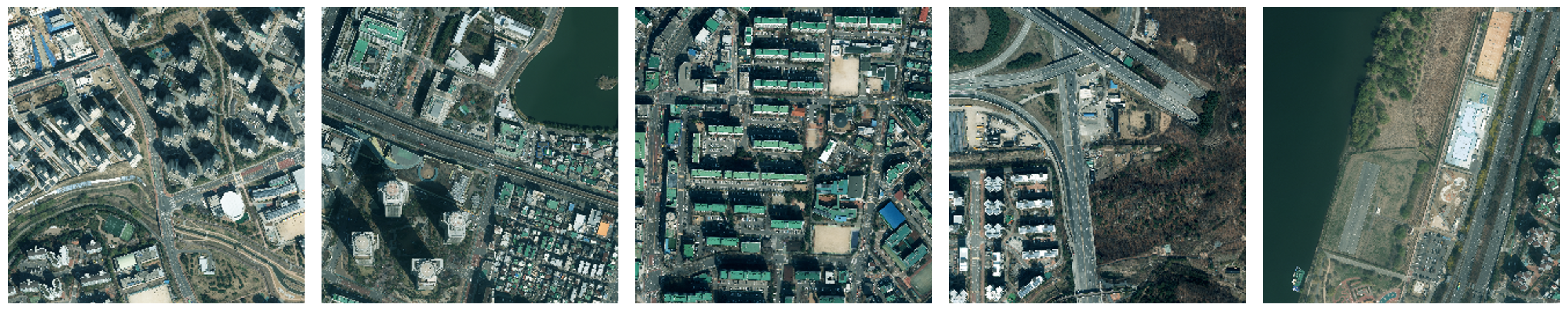
Aerial photos of Seoul were obtained from the National Geographic Information Institute (NGII, https://www.ngii.go.kr/eng/main.do, accessed on 14 June 2024). NGII produces various national geospatial images using high-resolution aerial photography technology. Aerial surveys are conducted every two years to create a comprehensive database of aerial photographs with a resolution of 25 cm. For this experiment, we used 141 images captured in April 2022. These images were first mosaicked into a single, geospatially aligned raster covering the entire study area. Then it was divided into grids with a spatial resolution of 512 m × 512 m, ultimately resulting in 2198 image tiles. Each tile was resampled to a 256 × 256-pixel resolution for model training. Figure 3 presents representative examples of these processed imagery tiles used as inputs to the model.

4.1.2. Sociodemographic Data

To incorporate sociodemographic information, data from the 2022 Population and Housing Census provided by the Statistical Geographic Information Service (https://sgis.kostat.go.kr/ accessed on 11 June 2024) were employed. The Population and Housing Census is one of the most fundamental and globally standardized national surveys. It represents Korea’s nationwide enumeration that covers the entire population and dwellings at a specific point in time. The survey collects general characteristics, such as population, households, housing units, number of business establishments, and employees, on a complete enumeration basis. Importantly, it offers data down to the local administrative level (eup, myeon, and dong), which can be spatially analyzed through its integration with Geographic Information Systems (GIS). In this study, census variables were utilized, including population counts, gender, age-group distributions, number of households, household types, number of establishments, and number of employees.

4.1.3. Public-Transit Ridership Data

Ridership data for different modes of transit in Seoul were obtained from the Seoul Open Data Plaza (https://data.seoul.go.kr/ accessed on 16 June 2024). The data include the average weekday ridership for 474 subway stations, 12,501 bus stops, and 2662 public bike rental stations in April 2022.

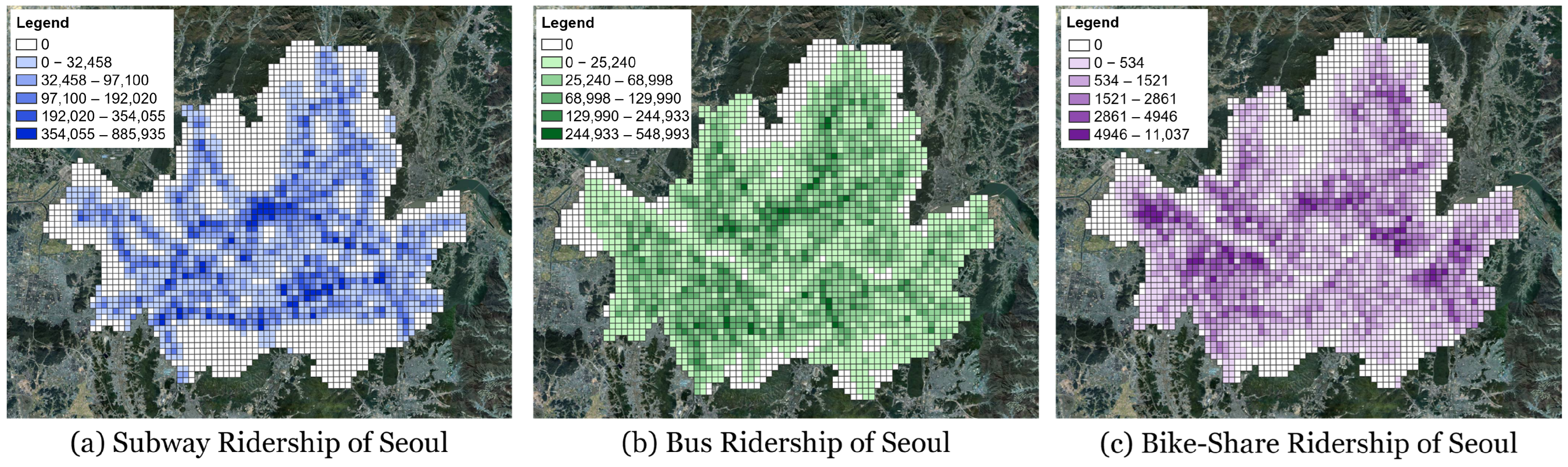
To reflect the ridership demand for each mode in different areas, Kernel Density Analysis (KDA) was applied to the usage data based on the stops. KDA is a useful analysis method for visualizing the density of geographically concentrated data points. We used boardings and alightings as weights. The bandwidth for the kernel was set to reflect the Pedestrian Catchment Area for each mode: 600 m for subways [22,35], 400 m for buses [36,37], and 300 m for public bikes [38,39,40]. Based on the KDA results for each mode, the KDA values for each cell were summed, and the ratio of each cell’s KDA value to the total KDA value was calculated. This ratio was then multiplied by the total capacity of each mode to reflect the density and actual ridership in each cell. Figure 4 visualizes the usage of each mode. To account for the significant variations in absolute usage volumes across different modes, Min–Max scaling was applied to normalize ridership values to a range between 0 and 1 for the training and validation datasets.

Table 1. Descriptive statistics of transit demand variables.

Category	Type	Mean	Std.	Min	25%	50%	75%	Max
Subway	Board	49,108	89,068	0	0	8585	62,544	885,935
	Alight	49,212	90,358	0	0	8358	62,172	886,440
Bus	Board	43,035	51,105	0	4388	29,814	59,787	548,993
	Alight	42,073	48,528	0	4652	30,252	60,311	572,287
Public Bike	Rentals	908	1240	0	25	441	1292	11,037

presents the descriptive statistics of transit ridership variables aggregated at the grid-cell level after applying Kernel Density Analysis. The results show substantial variation in both magnitude and distribution across transit modes. Subway demand exhibits the highest average and variability, with a mean of 89,068 boardings and 90,358 alightings per cell, but with medians below 9000. This indicates a highly skewed distribution concentrated in a few major stations. The maximum values exceed 880,000 passengers, while more than half of the cells record zero subway demand, reflecting extreme spatial imbalance.

Bus ridership shows moderate magnitudes and a less skewed pattern compared with subway demand. The average boarding and alighting volumes are approximately 51,105 and 48,528 passengers, respectively, with median values around 30,000. The minimum and lower-quartile values above zero suggest that bus usage is more evenly distributed across urban areas than subway usage.

Public bike rentals display the smallest scale and the largest relative variability. The mean number of rentals per cell is 1240, while the median is only 441, and the range extends up to 11,037. This indicates that public bike usage is concentrated in a limited number of active areas, with many cells showing few or no rentals.

Overall, these descriptive statistics reveal distinct spatial and numerical patterns among the three modes. Subway ridership is characterized by a large scale but extreme concentration, while bus demand is moderate and spatially dispersed. Public bike ridership is small in magnitude but highly localized. Such heterogeneity in data distribution implies that errors and model performances are likely to vary across transit modes in the subsequent analysis.

4.2. Experiment Architecture Setting

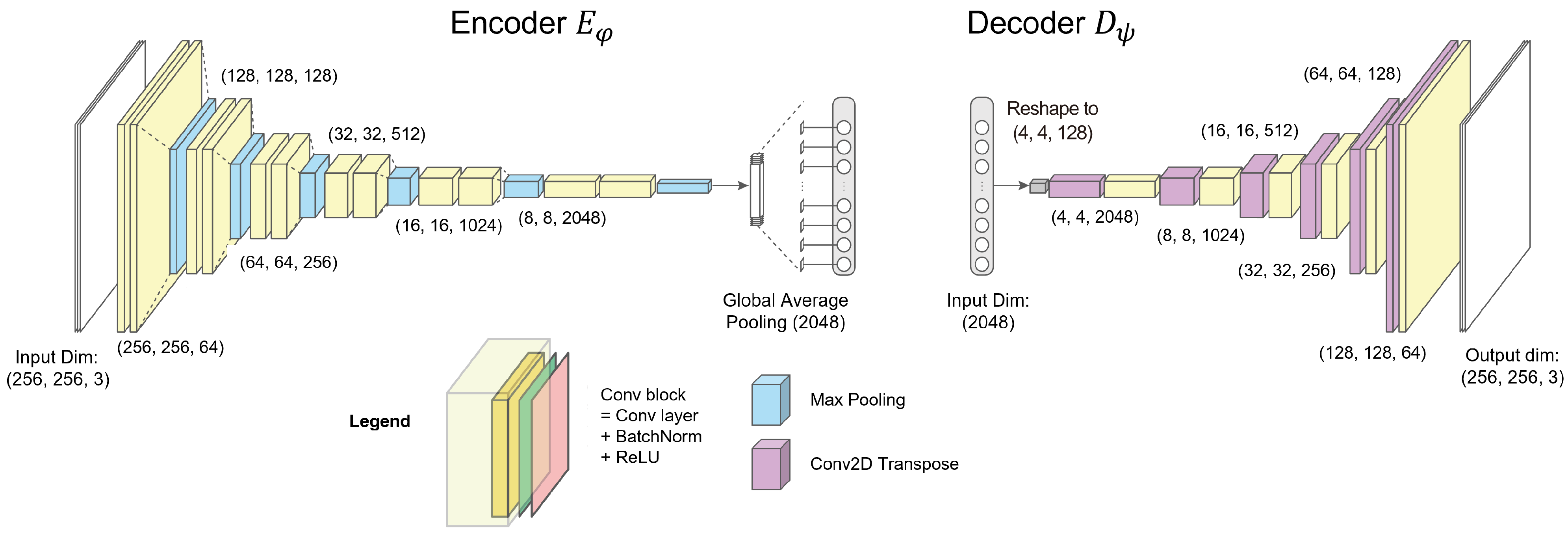
This section explains the model architecture used in the experiment. Figure 5 illustrates the complete architecture of the proposed model. The model consists of networks $E_{\omega }$ that predict $z_e$, $E_{\phi }$, and $D_{\psi }$ for learning $z_i$, and $N{N}_{\tau }$ to predict public transit demand using input vectors $z_e$ and $z_i$. The bottom-right panel provides a detailed view of the internal structure of $N{N}_{\tau }$, showing the sequence of fully connected layers, normalization, and activation functions used for transit demand prediction. Figure 6 illustrates the detailed architecture setting of $E_{\phi }$ and $D_{\psi }$.

The input image shape is 256 × 256 × 3, which is consistent across all sub-models. The basic structure of the encoder model consists of multiple layers defined as a convolutional block (Convolutional layer ($Nu{m}_{filters}$) + BatchNormalization + ReLU activation + MaxPooling) and a dense block (Dense layer ($Nu{m}_{units}$)) + BatchNormalization + ReLU activation). In the encoder blocks $E_{\omega }$ and $E_{\phi }$, there are six convolutional blocks. The number of filters in the convolutional layers for each block is 64, 128, 256, 512, 1024, and 2048, respectively. This is followed by a global average pooling layer that converts the output into a 2048 × 1-dimensional vector.

The increasing number of filters (from 64 to 2048) was chosen to capture the multi-scale spatial structures present in urban aerial imagery. Although the effective resolution of the input patches is 2 m/pixel, each 256 × 256 image covers a large and heterogeneous urban region containing diverse built-environment elements. Preliminary ablation tests indicated that reducing the maximum channel width noticeably degraded the quality of latent representations and reconstruction, so the 2048-filter configuration was adopted as a sufficient capacity for this task.

For $E_{\omega }$, the next layers consist of four dense blocks with 2048, 1024, 512, and 256 units, respectively. These are connected to the output layers with two units for gender prediction, eight units for age prediction, six units for household composition prediction, and eight units for other sociodemographic predictions. Except for the other sociodemographic output units that use ReLU activation, the rest use softmax activation to predict distributions.

In the sub-model learning $z_i$, $E_{\phi }$ connects directly to the output layer after global average pooling, resulting in an output dimension of 2048 × 1. The outputs of $E_{\phi }$ are concatenated through a concatenation layer. The combined 2072 × 1 vector then passes through a dense layer with 2048 units, reshaped into a 4 × 4 × 128 tensor, and subsequently processed through $D_{\psi }$, which is composed of decoder blocks defined as (ConvTranspose2D + Convolutional block) with filter numbers 2048, 1024, 512, 256, 128, and 64. The final output layer is a convolutional layer with three filters and a sigmoid activation function. Finally, in the sub-model $N{N}_{\tau }$, predicting public transit ridership, $z_e$ and $z_i$ are combined through a concatenation layer. As shown in the right corner of Figure 5, the concatenated vector is passed through three dense blocks with 128 units each, and connected to an output layer with six units and ReLU activation.

All models were trained using the Adam optimizer with a learning rate of 0.001 and a batch size of 32. The dataset was split using a fixed random seed (42), with 95% of the data used for training, 3% for validation, and 2% for testing, corresponding to 2088 training samples, 66 validation samples, and 44 test samples.

4.3. Experimental Model Configurations

Considering the limited research on predicting public transit ridership using remote imagery, our study proposes a novel approach that predicts ridership by extracting latent vectors from urban imagery to capture sociodemographic and physical environment features. Although evaluating the model’s performance against existing studies would be ideal, directly comparable research using urban imagery for public transit demand prediction is extremely limited. Prior studies differ widely in data modalities, spatial units, prediction targets, and modeling objectives, making a quantitative comparison of $R^2$ values infeasible. To address this limitation, the proposed model (Model 4) was compared with three alternative configurations (Models 1–3) through internal benchmarking. All four models share the same network architecture to ensure a fair comparison, differing only in the types of input data provided. This setup allows us to isolate and assess the impact of each data source—imagery, sociodemographic variables, and their combinations—on prediction performance.

Model 1 uses latent features extracted from the imagery, denoted as $z_i$, and the network is represented as $TB=N{N}_{\tau }\left(z_i\right)$. This model serves as a baseline to assess whether urban imagery features alone can effectively predict public transit ridership. It provides a reference point to evaluate the added value of integrating sociodemographic features into the prediction process. Model 2 uses only sociodemographic data as input $z_e$, following the structure $TB=N{N}_{\tau }\left(z_e\right)$. This model serves as a reference for comparison with traditional approaches. Model 3 combines both imagery-derived features $z_i$ and actual sociodemographic data $z_e$, allowing us to test whether combining these data sources improves performance. Model 4, the proposed model, uses imagery-derived $z_i$ and an estimated version of sociodemographic information ${\widehat{z}}_e$, reconstructed from imagery. The combined input $z_i+{\widehat{z}}_e$ is fed into the network, formulated as $TB=N{N}_{\tau }(z_i+{\widehat{z}}_e)$. This model is designed to explore whether public transit ridership can still be accurately predicted when actual sociodemographic data are unavailable, highlighting the potential for remote imagery to act as a proxy in data-scarce regions. These models are summarized in

Table 2. Model configurations.

Model	Input	Configuration
Model 1	$z_i$	$TB=N{N}_{\tau }\left(z_i\right)$
Model 2	$z_e$	$TB=N{N}_{\tau }\left(z_e\right)$
Model 3	$z_i\oplus z_e$	$TB=N{N}_{\tau }(z_e\oplus z_i)$
Model 4	$z_i\oplus {\widehat{z}}_e$	$TB=N{N}_{\tau }({\widehat{z}}_e\oplus z_i)$

. Model training was conducted using Google Colaboratory with Python 3.9 and TensorFlow 2.15.

4.4. Evaluation Metrics

We evaluated the predictive performance of the proposed models using three widely adopted regression metrics: Root Mean Square Error (RMSE), Mean Absolute Percentage Error (MAPE), and the Coefficient of Determination ($R^2$). Each of these metrics measures different aspects of model accuracy and stability, as formulated in Equations (8)–(10).

$$\mathrm{RMSE}=\sqrt{{\displaystyle \frac{1}{n}}\sum _{i=1}^n{(y_i-{\widehat{y}}_i)}^2}$$

(8)

where $y_i$ and ${\widehat{y}}_i$ denote the observed and predicted values, respectively. RMSE represents the average magnitude of prediction errors in the same units as the target variable. A lower RMSE indicates that the predictions are, on average, closer to the ground truth.

$$\mathrm{sMAPE}={\displaystyle \frac{100}{n}}\sum _{i=1}^n{\displaystyle \frac{2|y_i-{\widehat{y}}_i|}{|y_i|+|{\widehat{y}}_i|}}$$

(9)

sMAPE provides a symmetric, percentage-based measure of prediction error by normalizing the absolute difference between actual and predicted values to the average of their magnitudes. This formulation alleviates the excessive inflation observed in MAPE when actual values are close to zero and ensures balanced sensitivity across varying demand levels. However, sMAPE may still be unstable when both the actual and predicted values approach zero.

$$R^2=1-{\displaystyle \frac{{\sum }_{i=1}^n{(y_i-{\widehat{y}}_i)}^2}{{\sum }_{i=1}^n{(y_i-\overline{y})}^2}}$$

(10)

where $\overline{y}$ is the mean of the observed values. The $R^2$ metric measures the proportion of variance in the dependent variable that is explained by the model. Higher $R^2$ values, closer to 1, indicate stronger explanatory power.

RMSE and MAPE measure the absolute and relative magnitudes of prediction errors, respectively, while R-squared indicates the proportion of variance explained by the model. Together, these metrics provide a balanced evaluation of both explanatory power and prediction accuracy.

5. Results

5.1. Latent Vector $z_e$

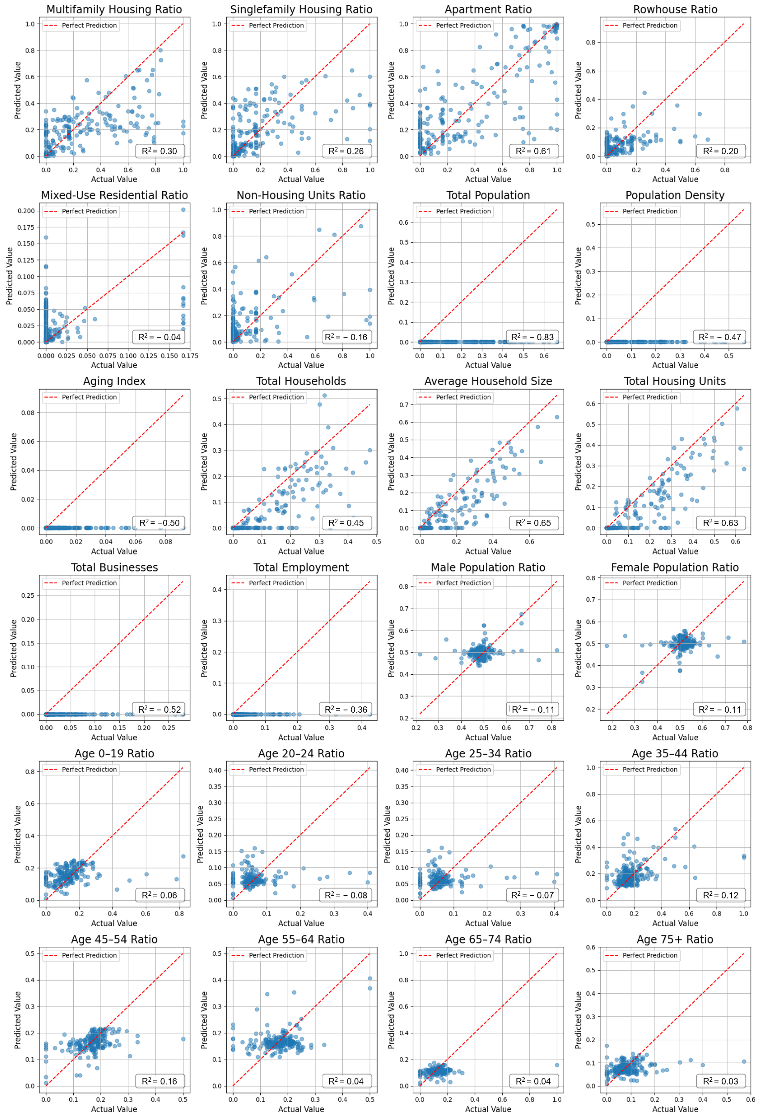
To assess whether the encoder $E_{\omega }$ effectively learns the socio-demographic latent vector $z_e$, the prediction results are evaluated with $R^2$ values. Figure 7 $z_e$ illustrates the predictive performance of 28 sociodemographic variables from aerial imagery.

The model exhibits strong predictive performance for variables related to housing and household structure, such as Apartment Ratio ($R^2$ = 0.61), Total Households ($R^2$ = 0.45), Total Housing Units ($R^2$ = 0.63), and Average Household Size ($R^2$ = 0.65). These variables reflect spatially organized residential patterns that tend to appear consistently in aerial imagery. Because these characteristics often co-vary with sociodemographic patterns, the encoder is able to infer them reliably from image features.

In contrast, variables representing population composition, such as sex ratios and age distributions, show limited predictive power. These variables are not directly observable from images; therefore, the model is unable to accurately predict them from visual cues alone. Some indicators like population density, employment, and business establishments show partial alignment but low overall $R^2$ due to skewed distributions, suggesting that the encoder captures certain spatial regularities but remains constrained by the information available in imagery.

Overall, the learned $z_e$ captures a meaningful subset of sociodemographic characteristics, particularly those that are spatially organized and indirectly reflected through residential patterns. Rather than encoding demographic composition directly, $z_e$ represents sociodemographic attributes that can be inferred from the spatial arrangement of households and residential forms.

5.2. Latent Vector $z_i$

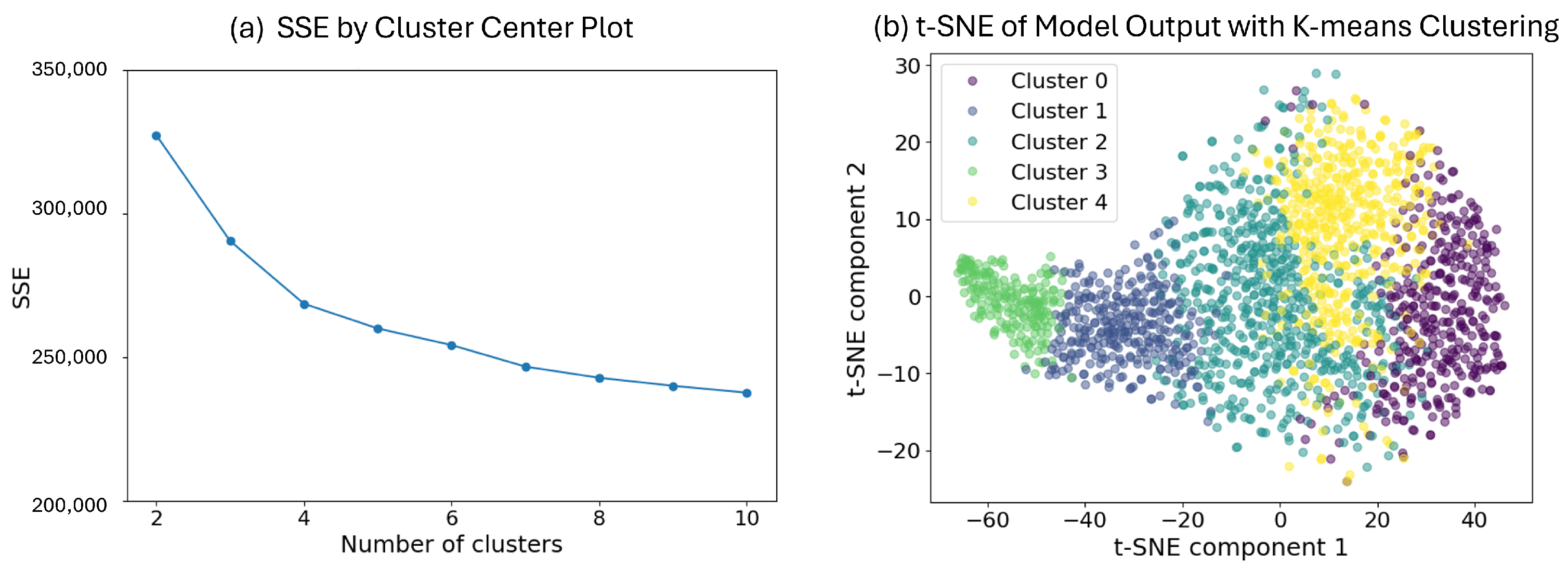
Unlike the $z_e$ latent vectors extracted using census data, we performed unsupervised learning on the $z_i$ vectors to encode the physical environmental attributes of the city. To understand the specific meaning of the $z_i$ vector, a cluster analysis was conducted using the vectors extracted from the images. Utilizing the k-means clustering method, five clusters were identified, as shown in Figure 8a. Additionally, we visualized the clusters using t-distributed stochastic neighbor embedding (t-SNE), a nonlinear dimensionality reduction technique, as illustrated in Figure 8b.

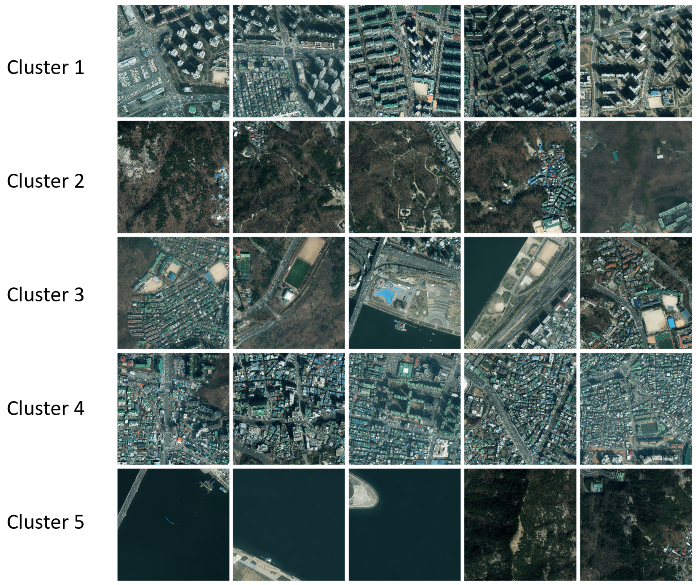
Each cluster consisted of images with similar $z_i$ vectors, indicating that these images share similar environmental characteristics. Figure 9 displays five randomly selected images from each cluster. To ensure methodological transparency, the images are presented in their original resolution for training and validation, with no up-scaling, smoothing, or other visual adjustments applied.

Cluster 1 consists of images with high-density buildings, such as apartments and mixed-use complexes. It represents areas with high population density within the city, typically large residential complexes or mixed-use buildings. A distinguishing feature of this cluster is the wider road widths compared to other image clusters. Next, Cluster 2 includes images of mountains, which represent natural environments within or surrounding the city. Cluster 3 has images with schools or parks predominantly from this cluster. It includes images with large open spaces, indicating public facilities or recreational areas. Cluster 4 consists of images from areas with densely packed buildings. It includes images with curved roads and is characterized by narrow streets and complex building layouts, reflecting traditional urban structures. Lastly, Cluster 5 comprises images of the Han River area or dark-colored mountain images, representing primarily waterfront areas or extensive natural environments. The outcomes of this cluster analysis indicate that the model effectively extracts physical environmental features from aerial imagery, allowing for the clustering of similar environments. This substantiates the validity of the image-based public transit ridership prediction model, implying that it is possible to make detailed ridership predictions that account for various physical environments within the city.

5.3. Model Performance Analysis

Table 3. Model performance comparison across transit modes.

Category	Metric	Model 1	Model 2	Model 3	Model 4
Subway
Board	$R^2$	−1.27	0.25	0.44	0.22
	RMSE	61,244	54,670	48,444	59,545
	sMAPE (%)	125.54	71.93	50.29	85.55
Alight	$R^2$	−0.02	0.15	0.38	0.18
	RMSE	63,991	57,267	49,217	59,941
	sMAPE (%)	126.70	74.09	52.11	85.85
Bus
Board	$R^2$	0.38	0.43	0.31	0.27
	RMSE	30,832	29,792	32,284	33,230
	sMAPE (%)	72.20	41.76	65.11	68.06
Alight	$R^2$	0.31	0.46	0.38	0.34
	RMSE	33,125	29,812	31,683	32,783
	sMAPE (%)	73.48	37.89	61.82	63.27
Public Bike
Rentals	$R^2$	0.42	0.56	0.61	0.31
	RMSE	1189	1048	979	1309
	sMAPE (%)	84.82	57.79	51.57	61.30

Note: Bold values indicate the best-performing model for each metric within the same category.

summarizes the predictive performance of four models across subway, bus, and public bike modes. Each block in the table represents one transit mode, and within each block, three evaluation metrics, mean absolute percentage error $R^2$, RMSE, and sMAPE are reported for boarding, alighting, or rental cases.

The four columns correspond to the four models introduced in Table 2. All results were obtained from the testing dataset at the epoch with the lowest validation loss. This study investigates the capability of image-derived information to predict public transit ridership without relying on actual sociodemographic data. In addition, comparing modes and models allows one to evaluate how image-based and sociodemographic features contribute to predictive performance in different travel contexts. The following sections provide a detailed comparison of predictive performance both across models and across transit modes to identify the strengths, limitations, and implications of each modeling approach. The predictive results yield the following three main findings.

First, Model 4 demonstrated improvement in predictive accuracy compared to Model 1. Across subway and public bike modes, Model 4 reduced both RMSE and sMAPE relative to Model 1. For subway, sMAPE decreases 31.8 percent and 126.70% for alighting and boarding, while RMSE also declines by 2.8% and 6.3%, respectively. Although the gains in $R^2$ are modest, the substantial reductions in percentage-based errors indicate that Model 4 captures relative variations much more effectively than Model 1. For the bus mode, boarding sMAPE decreases only modestly—a 5.7% reduction—but alighting accuracy improves more notably. sMAPE decreases by 13.9%, accompanied by an increase in $R^2$ and a slight reduction in RMSE from 33,125 to 32,783. Public bike ridership shows a similar pattern with sMAPE declining by 27.5%, although RMSE increases. These improvements suggest that incorporating an additional latent space that captures demographic-like patterns helps compensate for the absence of true sociodemographic variables.

Second, Model 3 achieved the highest overall performance for the prediction of the subway and public bike. By jointly using image-derived latent vectors and observed sociodemographic variables, Model 3 achieved the highest coefficients of determination. The $R^2$ values were 0.44 and 0.38 for subway boarding and alighting, and 0.61 for public bike rentals, with the lowest RMSE and sMAPE across these modes. For subway ridership, incorporating sociodemographic information significantly reduced prediction errors, with sMAPE decreasing from 125.54 to 50.29 for boarding and from 126.7 to 52.11 for alighting, representing reductions of approximately 60 and 59 percent. These improvements indicate that both population characteristics and built-environment features contribute substantially to explaining subway usage patterns. For public bike rentals, Model 3 achieved an R² of 0.61, improving prediction accuracy by roughly 60 percent compared to Model 1. This result suggests that high-resolution imagery effectively captures micro-level physical conditions, such as street design and cycling infrastructure.

Third, Model 2, which used only sociodemographic variables, provided the best performance for bus ridership. Specifically, bus alighting achieved the lowest RMSE, approximately 29,800, which is about 5.4% of the maximum ridership, and the lowest sMAPE, as well as the highest $R^2$ value, 0.46. This likely reflects the fact that bus usage patterns are closely tied to sociodemographic indicators, which are already well captured by traditional demographic data. Although this finding does not align directly with the primary goal of imagery-based modeling, it provides essential information on the explanatory power of different data types in different travel modes.

5.4. Model Performance Across Modes

The public bike mode demonstrates the most stable and accurate performance in terms of $R^2$, which is about 8% of the maximum ridership, the lowest MAPE, approximately 38%, and the highest R² value variation in bike rental ridership. The RMSE values, ranging from 979 to 1309, correspond to roughly 9–12% of the full demand range. The sMAPE values fall between 51.57 and 84.82 percent, which appear relatively high are largely due to the prevalence of low-demand or zero-demand subdistricts in the bike dataset. In such areas, even small absolute deviations inflate percentage-based errors because the denominator in sMAPE becomes very small. Nevertheless, the consistently high $R^2$ values, which were up to 0.61, and low RMSE values indicate that image-derived physical environment latent vector and sociodemographic features effectively capture the spatial heterogeneity of bike rental patterns.

The bus mode shows moderate predictive performance. The $R^2$ values range from 0.31 to 0.46, indicating that the model explains approximately 30 to 45% of the spatial variation in bus ridership across subdistricts. The RMSE values correspond from 5.4% to 6.1% of the maximum boarding volume and 5.2% to 5.8% of the maximum alighting volume, suggesting that the absolute prediction errors remain relatively small despite the moderate explanatory power. The sMAPE values range from 41.76 to 73.8%. These results suggest that while the models capture general spatial patterns of bus demand reasonably well, bus ridership is driven more strongly by demographic and behavioral factors. Consequently, the sociodemographic-only model, Model 2, yields the strongest performance for bus prediction, with limited additional benefits from incorporating image-based features.

The subway mode exhibits the most dramatic variation in model performance among all transit modes. This pattern reflects the highly skewed distribution of subway ridership, where a large share of subdistricts report zero or very low demand, while major transfer stations reach daily volumes exceeding 880,000. Such extremely long-tailed characteristics make the subway mode highly sensitive to model specifications. The physical environment latent vector-only model performs poorly, with negative $R^2$ values and very high sMAPE, indicating that built environment features alone cannot capture subway ridership. In contrast, incorporating socioeconomic variables produces substantial gains, improving $R^2$ to 0.44 for boarding and reducing sMAPE from over 125% to nearly 50%. The RMSE values for Model 3 correspond to only 5–6% of the maximum observed ridership, demonstrating high absolute accuracy despite the large magnitude of subway demand. Even Model 4, which extracts demographic-like latent features from imagery, provides substantial improvement over the image-only baseline, highlighting the importance of demographic patterns in explaining subway usage. Overall, subway ridership is strongly shaped by broad socioeconomic and population characteristics, which explains the dramatic performance differences observed across models.

6. Discussion

6.1. Implications and Interpretation

Model 3 remains the best-performing model; its strength stems from the availability of accurate, census-based sociodemographic data. In this sense, Model 3 illustrates the upper bound of how well the proposed framework can perform when rich auxiliary information is available. However, these data are not always accessible, up-to-date, or consistently collected across regions, which limits the scalability of such models in real-world applications. Model 4 addresses this limitation by demonstrating that a comparable level of performance can be achieved using only imagery-derived features, without requiring access to actual sociodemographic information.

The improvement from Model 1 to Model 4 is particularly meaningful. The relatively low performance of Model 1 likely results from the fact that raw image data do not explicitly encode sociodemographic attributes, making it difficult to capture key determinants of transit ridership. By learning to infer these characteristics through latent representations, Model 4 effectively narrows the performance gap between pure imagery-based and census-informed models. Although Model 4 does not reach the predictive accuracy of Model 2 or Model 3, it substantially outperforms Model 1, emphasizing the added value of sociodemographic representations extracted from urban imagery.

Importantly, the strong performance of Model 3, combining actual sociodemographic attributes with the physical environment latent vector $z_i$, also indicates the potential upper bound that could be achieved if both latent representations $z_e$ and $z_i$ were learned with higher fidelity. In other words, the gap between Model 3 and Model 4 reflects not a structural limitation of imagery-based approaches, but the current stage of latent feature learning. As the extraction of demographic-like signals in $z_e$ and physical environment patterns in $z_i$ improves, there is considerable room for the imagery-only model to approach the accuracy of census-informed models. This highlights significant potential for future research to enhance the latent space learning process and further strengthen imagery-based ridership forecasting.

The primary contribution of this study lies not in surpassing traditional models in data-rich environments but in demonstrating a scalable and transferable framework for estimating ridership in data-scarce or underrepresented regions. This approach offers a practical pathway for data-driven transit planning and decision-making in areas where conventional survey-based sociodemographic data are unavailable, outdated, or prohibitively costly to obtain.

6.2. Future Research Directions

There are several limitations to our model. The Separated Latent Vector Approach processes urban images using autoencoders and CNNs, and this powerful image interpretation capability is inevitably associated with a highly complex neural network structure. As a result, the following limitations may arise. First, the complex deep learning architecture requires significant computational resources, which can slow down training and inference, especially when dealing with large-scale datasets. This computational complexity may impose constraints on real-time data analysis or large-scale data processing. Second, deep learning models tend to converge to various local optima, raising the risk that the final solution may not be a global optimum. This risk becomes particularly significant when handling nonlinear and complex data structures, where the model might overfit specific regional patterns. These limitations are common challenges associated with complex neural network structures, and future advances in neural network models and optimization techniques will help overcome them. The model in this study represents an initial attempt to predict public transit ridership using images, and three potential avenues for further advancement have been identified for future research.

6.2.1. External Validity

Further research is needed to evaluate the applicability of the proposed model across various cities and environments. By capturing sociodemographic and physical environment features from images, the model can be expected to yield similar results in other regions. This capability could be particularly beneficial in areas like the Global South, where sociodemographic characteristics and development patterns vary significantly, but up-to-date census data are often lacking. Several approaches should be explored in future research to enhance the external validity of the model.

First, it is crucial to evaluate the model’s general applicability using diverse regional datasets. Including data from cities with differing traffic patterns, levels of development, and degrees of urbanization could help ensure that the model is not overly sensitive to regional characteristics and can be broadly applied. This will contribute to consistent performance across diverse environments.

In addition to expanding the geographic scope of the dataset, future work should also integrate more conservative validation strategies to ensure the robustness of the model’s generalizability across space. Approaches such as spatial block cross-validation, district-level holdout, and buffered spatial cross-validation would provide more reliable out-of-sample estimates and help guard against potential spatial leakage that may arise under random partitioning. Incorporating these evaluation strategies will be a key direction for improving the external validity and reliability of future models.

Third, incorporating pretraining into the model development process could be a valuable strategy. During the second stage of the proposed model, training $E_{\omega }$, pretraining with images from multiple regions could enable the model to extract more generalized image features. By leveraging datasets from areas with varying development patterns, pretraining could significantly improve the model’s predictive performance across different contexts.

Lastly, optimizing the model structure and experimental parameters is crucial for enhancing both predictive and generalization performance. While this study identified optimal parameters, as written in Section 4, aspects such as image resolution, grid size, and model architecture require further exploration. Higher-resolution images and smaller grids offer detailed insights but require more computational resources, whereas larger grids provide broader trends but may miss finer variations. Through these additional efforts, this study has the potential to evolve beyond the prediction of transit demand in specific cities, offering a more broadly applicable model with greater external validity.

6.2.2. General Transportation Demand

While this study focuses on public transit demand, we believe that the proposed model is not inherently limited to transit and could potentially be applied to general transportation demand prediction. For instance, in the case of Direct Ridership Models, the model could be adapted for other modes of transportation if sufficient data for those modes are available. Furthermore, the applicability of image data should be explored in existing frameworks for travel demand modeling, such as Sequential Demand Modeling and Activity-Based Modeling. As highlighted in previous studies, image data contains information about sociodemographic indicators and urban physical environments, making it a highly promising input variable for complementing quantitative data in these models. In Sequential Demand Modeling, particularly the 4-Step Travel Demand Modeling framework, image data could potentially be utilized in each stage of the process. A recent study that proposed a Deep Hybrid Model incorporating image data for mode choice prediction is particularly noteworthy in this context. The model demonstrated superior performance compared to traditional deep learning-based demand prediction approaches [41].

6.2.3. Multiple Data Modalities

This study was conducted to examine whether public transit demand can be predicted solely using image data. However, combining image data with other complementary datasets could further enhance the predictive performance of the model. Many studies have highlighted the potential of integrating non-structured data with other datasets, as extracting meaningful information from non-structured data can be challenging [42,43,44,45]. For public transit demand prediction, incorporating additional inputs such as the cost of transportation modes, travel time, and availability—key factors that directly influence transit usage—could significantly improve predictions. Future research could focus on enhancing the accuracy and comprehensiveness of transit demand models by integrating supply-related variables as additional inputs.

In summary, this study presents an innovative methodology for predicting public transit demand using urban imagery, confirming its potential utility. This framework can contribute significantly to urban planning and the formulation of public transit policies, especially in scenarios that involve the establishment of new transit stations in existing cities. Future research should investigate the extension of the model to different regions and cities, as well as explore its utility in general transportation beyond public transit. Additionally, incorporating diverse datasets as input variables and employing a broader range of models could further enhance the general applicability of the model.

7. Conclusions

Urban imagery offers valuable information for understanding sociodemographic characteristics and physical aspects of the urban environment in data-scarce regions. Despite their growing availability and potential, limited research has explored their use in predicting public transit ridership, which is a key element for sustainable transportation planning. This study proposed a novel framework that leverages urban imagery to extract two disjoint latent vectors: one representing sociodemographic features and the other capturing physical environmental characteristics, which are used to forecast public transit ridership.

The first objective of this study was to determine whether these two distinct types of information could be effectively disentangled through latent representations. The empirical results confirm that the proposed framework successfully achieves this separation. The sociodemographic latent vector captures spatially organized residential characteristics such as housing types, household structure, and residential density attributes that are indirectly reflected in aerial imagery. Meanwhile, the physical environment latent vector forms coherent clusters corresponding to dense urban districts, traditional street grids, open spaces, natural areas, and waterfront environments. These findings demonstrate that the model learns two functionally distinct latent spaces that meaningfully represent demographic-like and physical environment information.

Building on this foundation, the predictive evaluation reveals important differences across data sources and transit modes. Empirical results based on data from Seoul indicate that the model using actual sociodemographic data achieves the highest predictive accuracy. However, our proposed model, which relies solely on image-derived features, including an inferred representation of sociodemographic characteristics, shows substantial improvement over the image-only baseline. While it does not outperform census-informed models, it approaches their performance, demonstrating that meaningful sociodemographic signals can be captured from imagery alone.

Our proposed model provides several key benefits. First, it enables clear separation and preservation of information. By learning $z_e$ and $z_i$ separately, the model can more precisely reflect and reconstruct sociodemographic and image data, ensuring that each latent vector maintains its unique set of information while functioning complementarily. Secondly, functional separation of the latent vector improves the interpretability. Distinguishing $z_e$ from $z_i$ simplifies understanding of each vector’s representation, thereby enhancing the interpretability of the model’s predictions and offering valuable insights for urban planning and policy-making. Finally, because the framework relies on imagery rather than direct access to census or survey-based variables, it offers significant potential for use in data-scarce or rapidly changing urban environments. By reducing dependence on traditional sociodemographic datasets, which are often costly, infrequently updated, or unavailable, the proposed approach provides a practical and scalable foundation for future research that integrates multimodal urban data and advances mobility planning. This framework offers a scalable foundation for future research integrating multimodal urban data and advancing image-based approaches in transportation analysis.

References

1. Kaeoruean, K.; Phithakkitnukoon, S.; Demissie, M.G.; Kattan, L.; Ratti, C. Analysis of demand–supply gaps in public transit systems based on census and GTFS data: A case study of Calgary, Canada. Public Transp. 2020, 12, 483–516. [Google Scholar] [CrossRef] [Scilit]
2. Hoque, J.M.; Zhang, I.; Schmitt, D.; Erhardt, G.D. Are public transit investments based on accurate forecasts? An analysis of the improving trend of transit ridership forecasts in the United States. Transp. Res. Part A Policy Pract. 2024, 186, 104142. [Google Scholar] [CrossRef] [Scilit]
3. Diab, E.; Kasraian, D.; Miller, E.J.; Shalaby, A. The rise and fall of transit ridership across Canada: Understanding the determinants. Transp. Policy 2020, 96, 101–112. [Google Scholar] [CrossRef] [Scilit]
4. Neog, D.; Brown, J. Transit ridership growth in small urbanized areas: Lessons from seven US transit systems. J. Urban Plan. Dev. 2022, 148, 05021051. [Google Scholar] [CrossRef] [Scilit]
5. Urbanek, A.; Acedański, J.; Krawczyk, G. Depopulation or ageing? Decomposing the aggregate effects of projected demographic changes on urban transport systems. J. Transp. Geogr. 2023, 111, 103662. [Google Scholar] [CrossRef] [Scilit]
6. Shao, Q.; Zhang, W.; Cao, X.; Yang, J.; Yin, J. Threshold and moderating effects of land use on metro ridership in Shenzhen: Implications for TOD planning. J. Transp. Geogr. 2020, 89, 102878. [Google Scholar] [CrossRef] [Scilit]
7. Pasha, M.; Rifaat, S.M.; Tay, R.; De Barros, A. Effects of street pattern, traffic, road infrastructure, socioeconomic and demographic characteristics on public transit ridership. KSCE J. Civ. Eng. 2016, 20, 1017–1022. [Google Scholar] [CrossRef] [Scilit]
8. Chi, M.; Plaza, A.; Benediktsson, J.A.; Sun, Z.; Shen, J.; Zhu, Y. Big data for remote sensing: Challenges and opportunities. Proc. IEEE 2016, 104, 2207–2219. [Google Scholar] [CrossRef] [Scilit]
9. Zhao, J.; Deng, W.; Song, Y.; Zhu, Y. Analysis of Metro ridership at station level and station-to-station level in Nanjing: An approach based on direct demand models. Transportation 2014, 41, 133–155. [Google Scholar] [CrossRef] [Scilit]
10. Cardozo, O.D.; García-Palomares, J.C.; Gutiérrez, J. Application of geographically weighted regression to the direct forecasting of transit ridership at station-level. Appl. Geogr. 2012, 34, 548–558. [Google Scholar] [CrossRef] [Scilit]
11. He, Y.; Zhao, Y.; Tsui, K.L. Geographically modeling and understanding factors influencing transit ridership: An empirical study of Shenzhen metro. Appl. Sci. 2019, 9, 4217. [Google Scholar] [CrossRef] [Scilit]
12. Yan, X.; Liu, X.; Zhao, X. Using machine learning for direct demand modeling of ridesourcing services in Chicago. J. Transp. Geogr. 2020, 83, 102661. [Google Scholar] [CrossRef] [Scilit]
13. Shao, Z.; Tang, P.; Wang, Z.; Saleem, N.; Yam, S.; Sommai, C. BRRNet: A fully convolutional neural network for automatic building extraction from high-resolution remote sensing images. Remote Sens. 2020, 12, 1050. [Google Scholar] [CrossRef] [Scilit]
14. Cervero, R.; Murakami, J.; Miller, M. Direct ridership model of bus rapid transit in Los Angeles County, California. Transp. Res. Rec. 2010, 2145, 1–7. [Google Scholar] [CrossRef] [Scilit]
15. Mucci, R.A.; Erhardt, G.D. Evaluating the ability of transit direct ridership models to forecast medium-term ridership changes: Evidence from San Francisco. Transp. Res. Rec. 2018, 2672, 21–30. [Google Scholar] [CrossRef] [Scilit]
16. Pinho, P.; Lopes, M.; Altieri, M.; e Sá, F.M.; Silva, C.; Amante, A. The application of direct ridership models in the evaluation of the expansion of the Porto Light Rail Transit. Case Stud. Transp. Policy 2024, 18, 101282. [Google Scholar] [CrossRef] [Scilit]
17. Driscoll, R.A.; Lehmann, K.R.; Polzin, S.; Godfrey, J. The effect of demographic changes on transit ridership trends. Transp. Res. Rec. 2018, 2672, 870–878. [Google Scholar] [CrossRef] [Scilit]
18. Rahman, M.; Yasmin, S.; Faghih-Imani, A.; Eluru, N. Examining the Bus Ridership Demand: Application of Spatio-Temporal Panel Models. J. Adv. Transp. 2021, 2021, 8844743. [Google Scholar] [CrossRef] [Scilit]
19. Durning, M.; Townsend, C. Direct ridership model of rail rapid transit systems in Canada. Transp. Res. Rec. 2015, 2537, 96–102. [Google Scholar] [CrossRef] [Scilit]
20. Guo, R.; Huang, Z. Mass rapid transit ridership forecast based on direct ridership models: A case study in Wuhan, China. J. Adv. Transp. 2020, 2020, 7538508. [Google Scholar] [CrossRef] [Scilit]
21. Li, L.; Zhong, L.; Ran, B.; Du, B. Analysis of the relationship between metro ridership and built environment: A machine learning method considering combinational features. Tunn. Undergr. Space Technol. 2024, 144, 105564. [Google Scholar] [CrossRef] [Scilit]
22. Jun, M.J.; Choi, K.; Jeong, J.E.; Kwon, K.H.; Kim, H.J. Land use characteristics of subway catchment areas and their influence on subway ridership in Seoul. J. Transp. Geogr. 2015, 48, 30–40. [Google Scholar] [CrossRef] [Scilit]
23. Albert, A.; Kaur, J.; Gonzalez, M.C. Using Convolutional Networks and Satellite Imagery to Identify Patterns in Urban Environments at a Large Scale. In Proceedings of the 23rd ACM SIGKDD International Conference on Knowledge Discovery and Data Mining (KDD ’17), Halifax, NS, Canada, 13–17 August 2017; Association for Computing Machinery: New York, NY, USA, 2017; pp. 1357–1366. [Google Scholar] [CrossRef] [Scilit]
24. Pastorino, M.; Gallo, F.; Di Febbraro, A.; Moser, G.; Sacco, N.; Serpico, S.B. Multimodal Fusion of Mobility Demand Data and Remote Sensing Imagery for Urban Land-Use and Land-Cover Mapping. Remote Sens. 2022, 14, 3370. [Google Scholar] [CrossRef] [Scilit]
25. Khan, M.; Hanan, A.; Kenzhebay, M.; Gazzea, M.; Arghandeh, R. Transformer-based land use and land cover classification with explainability using satellite imagery. Sci. Rep. 2024, 14, 16744. [Google Scholar] [CrossRef] [Scilit] [PubMed]
26. Singleton, A.; Arribas-Bel, D.; Murray, J.; Fleischmann, M. Estimating generalized measures of local neighbourhood context from multispectral satellite images using a convolutional neural network. Comput. Environ. Urban Syst. 2022, 95, 101802. [Google Scholar] [CrossRef] [Scilit]
27. Baragwanath, K.; Goldblatt, R.; Hanson, G.; Khandelwal, A.K. Detecting urban markets with satellite imagery: An application to India. J. Urban Econ. 2021, 125, 103173. [Google Scholar] [CrossRef] [Scilit]
28. Putri, S.R.; Wijayanto, A.W.; Pramana, S. Multi-source satellite imagery and point of interest data for poverty mapping in East Java, Indonesia: Machine learning and deep learning approaches. Remote Sens. Appl. Soc. Environ. 2023, 29, 100889. [Google Scholar] [CrossRef] [Scilit]
29. Arshad, A.; Zulfiqar, J.; Zaib, M.H.; Khan, A.; Khan, M.J. Mapping socioeconomic conditions using satellite imagery: A computer vision approach for developing countries. J. Econ. Technol. 2023, 1, 144–163. [Google Scholar] [CrossRef] [Scilit]
30. Ayush, K.; Uzkent, B.; Burke, M.; Lobell, D.; Ermon, S. Generating Interpretable Poverty Maps using Object Detection in Satellite Images. arXiv 2020, arXiv:2002.01612. [Google Scholar] [CrossRef] [Scilit]
31. Dasgupta, N. Using satellite images of nighttime lights to predict the economic impact of COVID-19 in India. Adv. Space Res. 2022, 70, 863–879. [Google Scholar] [CrossRef] [Scilit]
32. Son, J.Y.; Lane, K.J.; Lee, J.T.; Bell, M.L. Urban vegetation and heat-related mortality in Seoul, Korea. Environ. Res. 2016, 151, 728–733. [Google Scholar] [CrossRef] [Scilit]
33. Zhang, C.; Wei, S.; Ji, S.; Lu, M. Detecting Large-Scale Urban Land Cover Changes from Very High Resolution Remote Sensing Images Using CNN-Based Classification. ISPRS Int. J. Geo-Inf. 2019, 8, 189. [Google Scholar] [CrossRef] [Scilit]
34. Fu, Y.; Chai, H.; Zhen, Z.; Wang, F.; Xu, X.; Li, K.; Shafie-Khah, M.; Dehghanian, P.; Catalão, J.P. Sky image prediction model based on a convolutional auto-encoder for minutely solar PV power forecasting. IEEE Trans. Ind. Appl. 2021, 57, 3272–3281. [Google Scholar] [CrossRef] [Scilit]
35. Li, S.; Yang, H.; Zhang, G.; Ling, Z.; Xiong, Y.; Li, Y. What is the best catchment area of a metro station? A study based on station level ridership modeling. In Proceedings of the 2019 5th International Conference on Transportation Information and Safety (ICTIS), Liverpool, UK, 14–17 July 2019; IEEE: Piscataway, NJ, USA, 2019; pp. 1239–1244. [Google Scholar]
36. Noh, N.M.; Mohamad, D.; Hamid, A.H.A. Acceptable walking distance accessible to the nearest bus stop considering the service coverage. In Proceedings of the 2021 International Congress of Advanced Technology and Engineering (ICOTEN), Virtual, 4–5 July 2021; IEEE: Piscataway, NJ, USA, 2021; pp. 1–7. [Google Scholar]
37. Mulley, C.; Ho, C.; Ho, L.; Hensher, D.; Rose, J. Will bus travellers walk further for a more frequent service? An international study using a stated preference approach. Transp. Policy 2018, 69, 88–97. [Google Scholar] [CrossRef] [Scilit]
38. Kabra, A.; Belavina, E.; Girotra, K. Bike-share systems: Accessibility and availability. Manag. Sci. 2020, 66, 3803–3824. [Google Scholar] [CrossRef] [Scilit]
39. Zhang, G.; Yang, H.; Li, S.; Wen, Y.; Li, Y.; Liu, F. What is the best catchment area of bike share station? A study based on Divvy system in Chicago, USA. In Proceedings of the 2019 5th International Conference on Transportation Information and Safety (ICTIS), Liverpool, UK, 14–17 July 2019; IEEE: Piscataway, NJ, USA, 2019; pp. 1226–1232. [Google Scholar]
40. Zhang, Y.; Thomas, T.; Brussel, M.; Van Maarseveen, M. Exploring the impact of built environment factors on the use of public bikes at bike stations: Case study in Zhongshan, China. J. Transp. Geogr. 2017, 58, 59–70. [Google Scholar] [CrossRef] [Scilit]
41. Wang, Q.; Wang, S.; Zheng, Y.; Lin, H.; Zhang, X.; Zhao, J.; Walker, J. Deep hybrid model with satellite imagery: How to combine demand modeling and computer vision for travel behavior analysis? Transp. Res. Part Methodol. 2024, 179, 102869. [Google Scholar] [CrossRef] [Scilit]
42. Cao, R.; Zhu, J.; Tu, W.; Li, Q.; Cao, J.; Liu, B.; Zhang, Q.; Qiu, G. Integrating Aerial and Street View Images for Urban Land Use Classification. Remote Sens. 2018, 10, 1553. [Google Scholar] [CrossRef] [Scilit]
43. Davenport, F.M.; Harrison, L.; Shukla, S.; Husak, G.; Funk, C.; McNally, A. Using out-of-sample yield forecast experiments to evaluate which earth observation products best indicate end of season maize yields. Environ. Res. Lett. 2019, 14, 124095. [Google Scholar] [CrossRef] [Scilit]
44. Li, T.; Xin, S.; Xi, Y.; Tarkoma, S.; Hui, P.; Li, Y. Predicting multi-level socioeconomic indicators from structural urban imagery. In Proceedings of the 31st ACM International Conference on Information & Knowledge Management, Atlanta, GA, USA, 17–21 October 2022; pp. 3282–3291. [Google Scholar]
45. Yeh, C.; Perez, A.; Driscoll, A.; Azzari, G.; Tang, Z.; Lobell, D.; Ermon, S.; Burke, M. Using publicly available satellite imagery and deep learning to understand economic well-being in Africa. Nat. Commun. 2020, 11, 2583. [Google Scholar] [CrossRef] [Scilit]
Figure 1. The concept of the model.
Sustainability 18 00067 g001
Figure 2. Model implementation process.
Sustainability 18 00067 g002
Figure 3. Image samples of aerial imagery.
Sustainability 18 00067 g003
Figure 4. Public transit ridership of Seoul.
Sustainability 18 00067 g004
Figure 5. Complete model architecture.
Sustainability 18 00067 g005
Figure 6. Experiment architecture of the image encoder–decoder network.
Sustainability 18 00067 g006
Figure 7. Scatter plots of predicted versus actual values of z e . Blue dots represent individual samples from the test dataset.
Sustainability 18 00067 g007
Figure 8. Cluster analysis on the latent vector z i .
Sustainability 18 00067 g008
Figure 9. Example imagery of each cluster.
Sustainability 18 00067 g009