Analysis of Factors Affecting Electric Vehicle Range Estimation: A Case Study of the Eskisehir Osmangazi University Campus

Abstract

In recent years, electric vehicles have become increasingly widespread, both in the logistics sector and in personal use. This increase, together with factors such as environmental concerns and government incentives, has brought energy consumption and range estimation issues to the forefront. In this study, the energy consumption of an electric cargo vehicle under different speed and load conditions is examined with an experimental and data-driven approach, and then used for range estimation. The raw data collected from the vehicle on the selected ~2 km route in Eskisehir Osmangazi University campus are combined into per-second samples with time synchronization and data cleaning. The route is divided into average of 150 m segments, and variables such as slope, energy consumption, and acceleration are calculated for each segment. Then, the data are used to train various machine learning models, such as Extra Trees, CatBoost, LightGBM, Voting Regressor, and XGBoost, and their performances regarding energy consumption-based range estimation are compared. The findings show that driving dynamics such as high speed and sudden acceleration, as well as road slope and load conditions, significantly shape the energy consumption and thus the remaining range. In particular, Extra Trees outperforms other machine learning models in terms of metrics such as R², RMSE and, MAE, with a reasonable computational time. The results provide applicable guidance in areas such as route optimization, smart battery management, and charging infrastructure to reduce range anxiety and increase the operational efficiency of electric vehicles.

1. Introduction

The transportation sector contributes significantly to greenhouse gas emissions. Fossil fuel vehicles have been recognized as one of the biggest contributors to climatic pollution, accounting for 23% of total energy-related CO₂ emissions [1]. Technological advances, environmental concerns, and government incentives have driven a significant increase in the adoption of electric vehicles, both for personal use and in logistics. All over the world, governments and authorities are working on strategies that will allow for a faster take-up of electric vehicles, along with enhancements in the charging facilities available [2].

An advantage of electric vehicles is they do not emit greenhouse gases or other pollutants when they are in operation. This will inevitably help to minimize the damage to the climate imposed by transportation as a whole [3]. Moreover, if electric vehicles are fuelled by renewable sources of energy, this would decrease the transportation sector’s adverse effects on the environment even further [4]. Adopting e-vehicles comes with more than just environmental perks. Economically, it can help to save operating costs for both consumers as well as businesses. As electric vehicles do not involve any mechanical parts and oil changing, these vehicles do not need as much service as vehicles using internal combustion engines. In addition, the cost of electric vehicles is relatively less volatile than the prices of gasoline, which enables better budgeting [5]. The growth in the electric vehicle industry is driving economic and innovation growth in the field of automobile manufacturing, battery development, and charging station development. In addition to these economic benefits, environmental benefits have led to the rapid spread of electric vehicles in various transportation sub-sectors.

Switching to electric vehicles offers numerous economic and environmental benefits. However, the transition to electric vehicles also brings with it several problems that need to be worked on. Short driving ranges due to battery capacity limitations and limited charging infrastructures are causing range anxiety among drivers [6]. Range anxiety becomes especially evident on long journeys, and makes planning difficult for users. It can become even worse due to a change in driving range caused by factors affecting energy consumption that are beyond the driver’s control. Therefore, accurate estimation of the range constitutes an important research topic in order to increase user confidence and optimize operational activities in electric vehicles. On the other hand, high-accuracy range estimation in the logistics sector helps to reduce costs by positively affecting energy efficiency, productivity, and route planning quality as it ensures optimum use of existing resources. In addition to this, it will inform infrastructure planning—in particular, the strategic placement of charging stations—and underpin the development of smart battery management.

In recent years, various studies have begun to be published in the literature on the range estimation of electric vehicles. Range estimation is a rather complex phenomenon that is directly related to energy consumption and is influenced by multiple factors that are related or unrelated to each other. Vehicle speed and acceleration are the primary determinants of energy consumption; higher speeds and sudden accelerations increase aerodynamic drag and mechanical load, respectively [7]. The road gradient plays an important role in energy consumption, due to the gravitational force acting on the vehicle. Uphill ascending scenarios require more energy, while descending scenarios can provide energy recovery, thanks to regenerative braking [8]. In addition to the weight of the vehicle, the weight of the passengers and the load carried also have a significant impact on the energy consumption of electric vehicles, especially during acceleration and uphill driving [9]. Vehicle speed, acceleration, road slope, and load are factors that have been addressed in separate studies in relation to energy consumption. However, how these interact—especially for short-haul segments—remains poorly understood. To address these challenges and advance the understanding of factors influencing energy consumption and range estimation in electric vehicles, this study adopts a focused approach on short-distance logistics, providing valuable insights for both theoretical frameworks and practical applications. The main objective of the study focuses on the range estimation of electric vehicles based on the energy consumed in real-life conditions, by systematically examining the factors affecting energy consumption. The dataset used in this study is created using a real electric cargo delivery vehicle. The main contributions of this study can be summarized as follows:

• It focuses on the energy consumption and remaining range estimation for a small three-wheeled electric vehicle designed for use in last-mile delivery logistics. In this context, it aims to determine the critical role of such vehicles in energy management and to increase the sustainability of logistics operations.
• In order to systematically observe the effects of slope, speed, load, and acceleration factors on energy consumption, an experimental design is established. The effects of particular factors that cause energy consumption are examined.
• Experiments are carried out with an electric vehicle used in real-life cargo delivery. This implementation increases the validity of the research by verifying the designed experiment in real-life conditions and helping to observe the effects of driving dynamics and environmental factors.
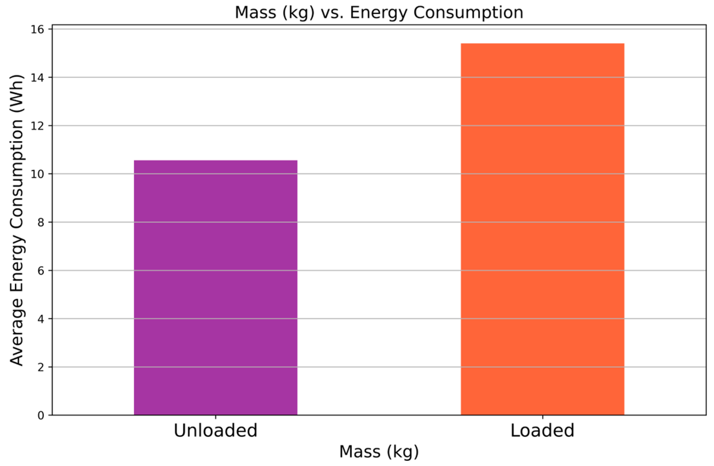
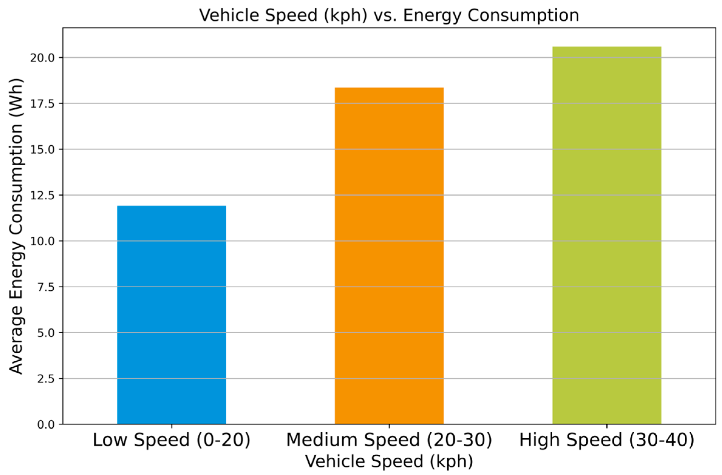
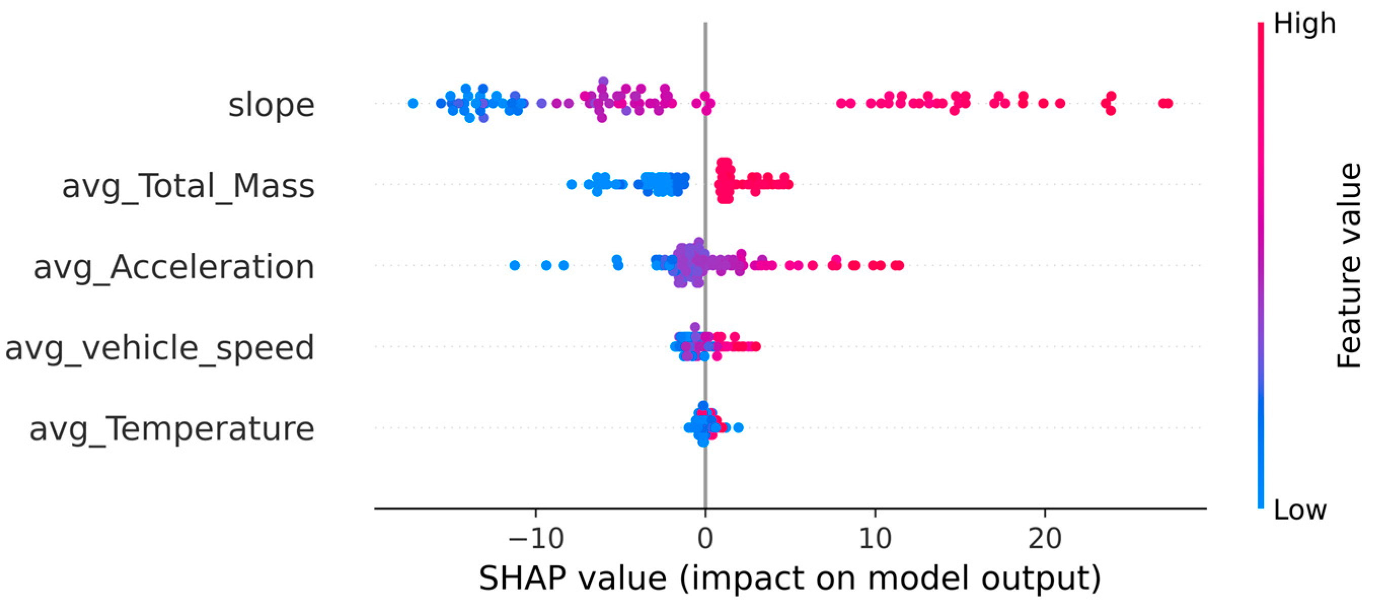
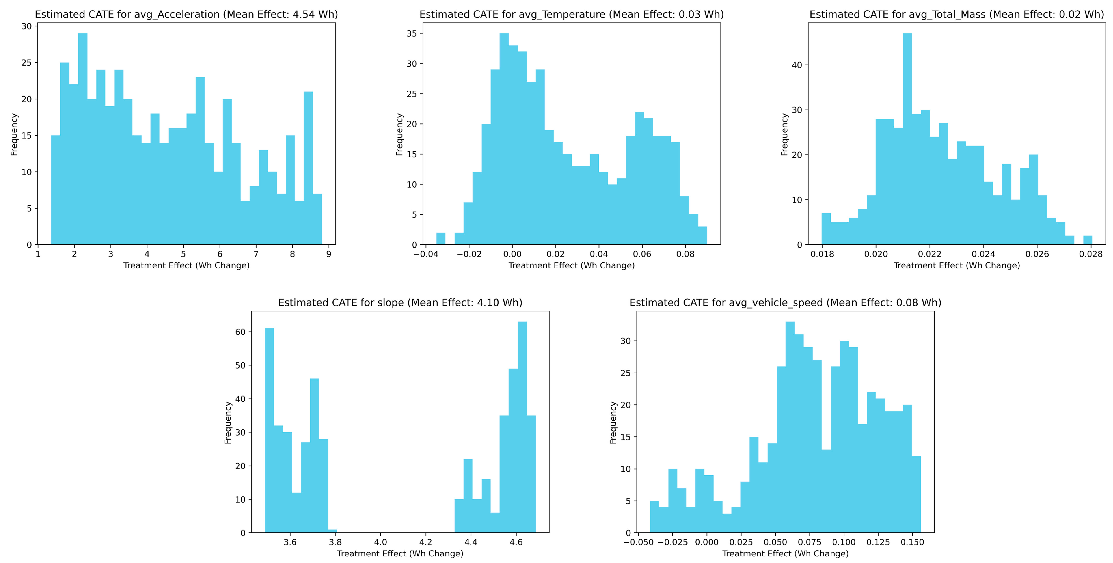
• The effects of slope, speed, load, and acceleration factors on energy consumption are statistically analyzed. The separate effects of each factor are explained, and ideas about the vehicle’s energy consumption and the estimation of the remaining range are presented.
• As one of the rare studies in the literature investigating the effect of the characteristics of small-scale regions on energy consumption, it emphasizes the effect of local factors on electric vehicle performance.
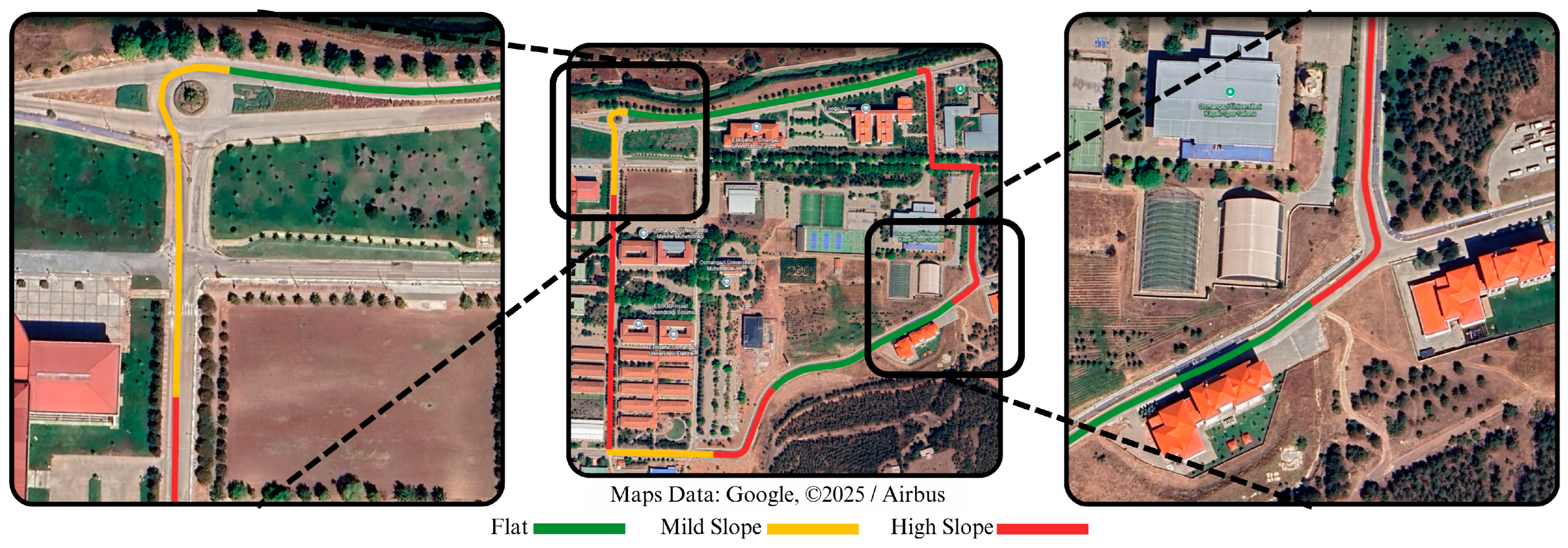
• In this context, the energy consumption analysis is carried out by focusing on shorter road segments with an average length of 150 m. This approach allows the dynamic changes in driving conditions and their immediate effects on energy consumption to be realized more precisely. For each road segment, the energy consumption is calculated using the State of Charge (SoC) value of the battery at the starting and ending points of the road segment. The relationship of energy consumption with specific factors in each segment provides valuable information about how these factors affect energy consumption and range. The remainder of the paper is organized as follows: Section 2 presents the related works, focusing on factors and algorithms used in the prediction of energy consumption and range estimation of electric vehicles. The dataset and the methodology used in the study are given in Section 3. Section 4 presents the experimental results and identifies the factors affecting the prediction of range. Finally, the discussions, conclusions, and suggestions for future work are presented in Section 5.

2. Related Studies

Concerns about fossil fuel depletion and increasing air pollution have led to an increase in the search for alternatives to internal combustion engine (ICE) road transport [10]. This has driven the increasing popularity of electric vehicles (EVs). However, the actual driving range of EVs is often significantly shorter, due to fewer charging facilities and longer charging times compared to ICE vehicles. As there are fewer EV charging points than fuel stations, EV drivers are constantly worried about arriving at their destination on time, making range anxiety inevitable [11]. Therefore, accurately determining how far an EV can travel on a single charge is important for EV drivers. A review of the literature shows that changes in driving conditions, driver behaviour, ambient conditions, and battery health lead to difficulties in accurately estimating the remaining range in electric vehicles. Existing studies highlight the need for advanced prediction models and real-time data integration to improve range prediction accuracy and develop effective battery management strategies in response to dynamically changing environmental conditions. Vaz et al. propose a multi-objective optimization technique. The technique shows the ideal driving speeds corresponding to the estimated range for the driver by increasing the electric motor efficiency and reducing the power consumption [12]. In the model-based approach, where the driving profile and power consumption are estimated, the remaining range estimation is achieved with an error of 2.52% [13]. In the study of Sarrafan et al., the researchers use environmental and drive system loss factors to estimate the State of Charge (SoC), and thus the EV range [14]. However, the SoC calculation is found to be more accurate, with only 0.5% difference between the estimated and measured value at the destination. The effect of driving efficiency on SoC is studied by Helmbrecht et al. [15]. They observe that customers with a lower SoC tend to change their driving habits to maintain the SoC.

In physical models, accurate measurements of many parameters, such as air resistance, rolling resistance, and slope force, are required. The variability of these parameters under different vehicle types and driving conditions limits the accuracy of the models [16,17,18,19]. Model-based range prediction is specific to EVs and requires prior knowledge of the battery. In recent years, data-driven machine learning-based approaches have been widely used to directly estimate the remaining driving range of electric vehicles [20]. Therefore, a more generalized range prediction algorithm that can help with different driver characteristics can be developed using data-driven machine learning algorithms. ML methods can learn complex and nonlinear relationships over data, independently of physical principles. In this way, sudden changes in driving conditions and the effects of environmental factors can be captured more accurately [21]. ML methods offer a more flexible structure compared to physical models that remain limited due to high data requirements and fixed assumptions. They can integrate dynamic factors such as road conditions into the model by learning from large and heterogeneous datasets. Interpretive techniques such as Shapley Additive exPlanations (SHAP) can show which variables are most effective in prediction, increasing the reliability of the model and its usability in practice. Data-driven algorithms can be modelled to accommodate different factors that may affect range consumption. Thus, they can be applied in situations where accurate mathematical modelling of the EV battery is difficult [22]. They also show great scalability, due to their robustness to noise and lower prediction error in range [23]. On the other hand, there are extensive studies in the literature on statistical, predictive, and causal analysis of factors affecting energy consumption under different driving conditions. For example, Huang et al. examined the factors affecting energy consumption of electric vehicles (EVs) in statistical, predictive, and causal dimensions. They investigated the role of these factors in different trip categories with the double-biased machine learning (DML) approach [24]. Gurusamy et al. focused on predicting the energy consumption of electric two-wheelers (E2Ws) using automatic Machine Learning (autoML) libraries. They showed that ensemble-based models increased the prediction accuracy, and especially, the PyCaret-based stacked ensemble model exhibited the best performance [25]. Yılmaz et al. proposed a transformer-based method for estimating the SoC. The study demonstrated the remarkable effectiveness of the transformer model for SoC prediction across various datasets [26]. Lee and Wu developed a big data framework to improve the driving range prediction of EVs using a single battery cell [27]. Sarrafan et al. used web-based data and driving behaviours for range estimation, and found an estimation error of 1% [28]. In the data-driven approach using the fuzzy logic classifier using battery parameters and consumed power, an error range of 20% was estimated [29]. Rhode et al. propose a data-driven approach for range estimation that adapts to changing conditions in real time, without relying on specific vehicle parameters [30]. Zhao et al. propose a hybrid machine learning algorithm combining XGBoost and Light Gradient Boosting Machine (LightGBM) methods, which can predict the remaining driving range for EVs using real driving data [31]. They find that the hybrid model reduces the prediction errors by an average of 20 km compared to traditional methods, and achieves an average absolute error of 10 km in range prediction. Tian et al. present a model combining and dimensionality extension approach using the eXtreme Gradient Boosting (XGBoost) technique to accurately predict the remaining range of electric vehicles [32]. The XGBoost model demonstrates superior performance compared to other machine learning methods by achieving a 15% increase in prediction accuracy. Zamee et al. propose a method for intelligent charging load estimation of EVs [33]. This method divides EVs into four categories: electric private cars, electric public transport buses, electric car rentals, and battery-powered vehicles for delivery. The system establishes charging power calculation models for various types of EVs and studies probabilistic models of load-influencing factors. Based on the estimated EV ownership, initial charging condition, and charging duration, the approach calculates the charging demand of EVs using Monte Carlo simulation. The study found that EV rentals, on average, increased their range by 50 km after charging to 80% SoC. Dong et al. propose a cascaded neuromorphic computation system that includes a Gated Recurrent Unit (GRU), an attention circuit module, and a Kalman filter to increase the speed and accuracy of SoC estimation [34]. The method both increases the accuracy and reduces the computation time by approximately 16 to 20 times. Selvaraj and Vairavasundaram propose a machine learning model approach based on Bayesian optimization, which considers environmental and in-vehicle factors to increase accuracy in SoC estimation [35]. The proposed model with high performance has a prediction error below 1%. Mishra et al. review machine learning models for range estimation in their study [36]. They emphasize the importance of data pre-processing techniques and model selection for accurate estimations. They observe that the use of algorithms such as Deep MLP and Random Forest provide higher accuracy in range estimations.

When the literature is examined, it can be seen that slope, acceleration, speed, and load factors are considered in most of the studies on energy consumption and range prediction (

Table 1. Factors examined in related works.

RW	Slope	Acceleration	Speed	Load	Model
Topić, Škugor, and Deur, 2019 [37]		√	√		DD
Varga, Sagoian, and Mariasiu 2019 [38]	√	√	√	√	DD
López and Fernández, 2020 [39]			√		PM
Miri, Fotouhi, and Ewin, 2021 [40]	√	√	√	√	PM, DD
Ullah, Liu, Yamamoto, Zahid, and Jamal, 2021 [41]	√		√	√	DD
Kocaarslan et al., 2022 [42]	√	√	√	√	PM
Sun, An, Geng, and Geng, 2023 [43]		√	√		PM
Achariyaviriya et al., 2023 [44]	√	√	√		DD
Yılmaz and Yagmahan, 2024 [45]	√		√	√	DD
Wang et al., 2024 [46]	√		√		DD
Gioldasis, Christoforou, and Katsiadrami, 2024 [47]	√		√		DD
Kozłowski, Wiśniowski, Gis, Zimakowska-Laskowska, and Borucka, 2024 [48]		√	√		PM
Our work	√	√	√	√	PM, DD

Our study addresses related factors. In addition, the factors are examined with both physical model (PM) and data-driven (DD) methods.

).

3. Materials and Methods

The increasing use of electric vehicles in the logistics sector has increased the importance of studies on the energy consumption and range of cargo vehicles. In this context, a new method is proposed to examine the factors affecting the range of an electric vehicle by implementing different scenarios. Scenarios were created in a real test environment and using data collected from an electric cargo delivery vehicle. The flow diagram of the proposed method is shown in Figure 1.

The research methodology presented in Figure 1 consists of three main phases: scenario definition, data collection and pre-processing, and analysis and validation. In the first phase, routes with different slope conditions are created at Eskisehir Osmangazi University Meselik Campus. The conditions to be tested, namely different speeds, different slope values, different temperature conditions, and different load cases, are determined. In the second phase, vehicle sensor data are collected, synchronized, and cleaned on a per-second basis. Routes are divided into segments based on slope, the appropriate slope value is assigned to each segment, and the data are normalized. In the last phase, the correlations of the factors affecting energy consumption are examined with the obtained dataset, energy consumption and range estimates are made with machine learning (ML) models, and the performances of these models are evaluated.

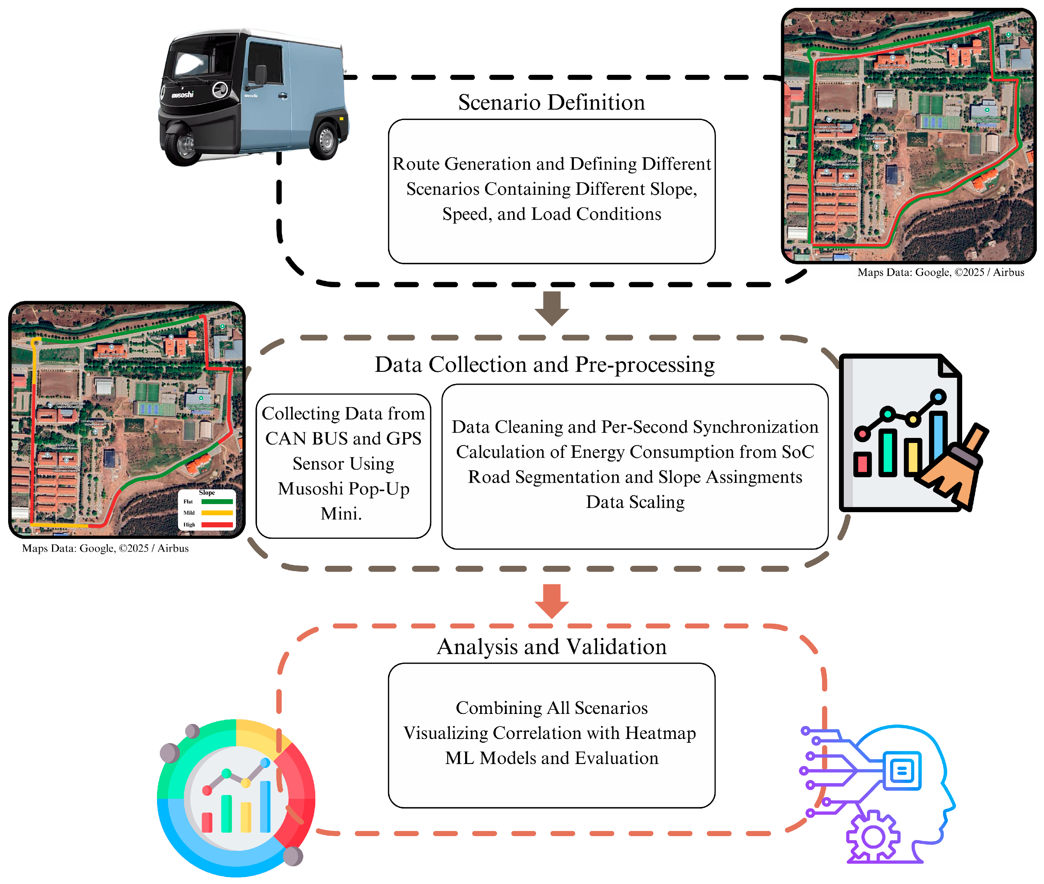
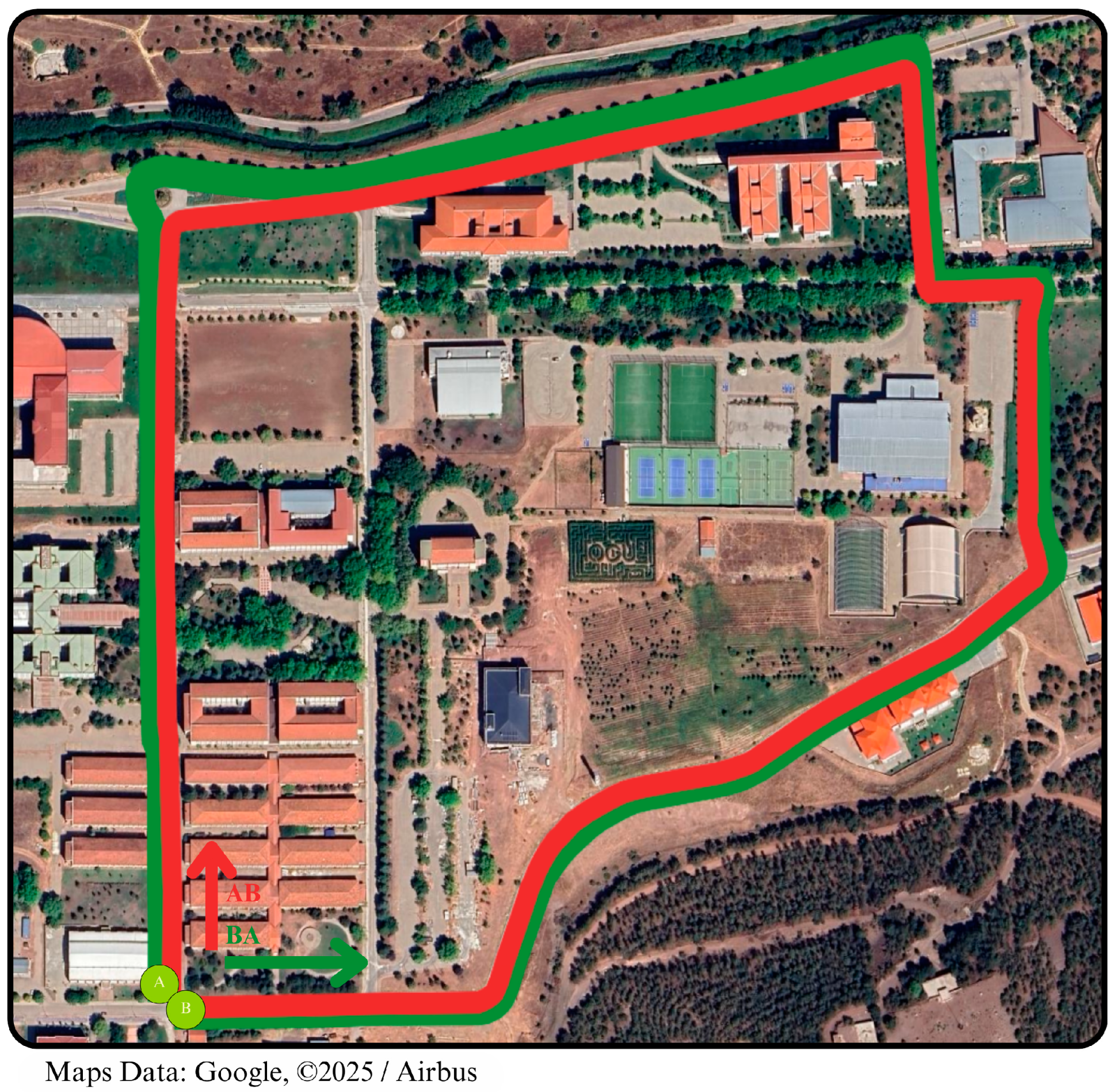
3.1. Scenario Definition

In this study, the effects on energy consumption and range were analyzed by collecting data under different speed, slope, weather, and load conditions from a Musoshi brand Pop-Up Mini electric vehicle. The parameters of the vehicle are given in

Table 2. Musoshi Pop-Up Mini parameters.

Description	Value
Vehicle Mass	700 kg
Payload Capacity	400 kg
Top Speed	50 km/h
Acceleration	1 m/s2
Range	120 km
Battery Capacity	15.6 kW/h
Front Surface Area	2.55 m2

.

The experiments were carried out on a route approximately 2 km in length, with slope values varying between 0% and 9%, in Eskisehir Buyukdere Neighbourhood, where Eskisehir Osmangazi University Meselik Campus is located (Figure 2). The reason for choosing this route was that different slopes and road conditions are presented in the same area, thus enabling data appropriate for real driving conditions to be obtained. Within the scope of the tests, the route was covered at an average speed of 15, 25, and 35 km/h in both the direction of travel and return. In addition, the vehicle was tested under two different load conditions (empty and 350 kg-loaded) for each speed option, and the tests were conducted in both the winter and summer seasons. In this way, the data for each speed and load combination were recorded separately; as a result, a total of 24 different experimental data files were obtained. These experiments were performed to minimize possible sensor errors and variations due to environmental variables. The experiments allowed for the systematic examination of changes in energy consumption and range estimation under various driving conditions.

While naming these routes, intelligent naming was used according to the speed, load, and direction. The numbers 15, 25, and 35 represent speeds, L represents loaded, and U represents unloaded. The letters M and C represent the direction towards The Faculty of Engineering and Architecture (represented as AB) and the direction towards The Center of Intelligent Systems Application Research (represented as BA), respectively. This wide range of data obtained provided the opportunity to examine in detail the performance and energy consumption of the vehicle under different conditions, in terms of variables such as speed, load, and slope. Thus, a comprehensive evaluation could be made in terms of driving dynamics and energy efficiency.

3.2. Data Collection and Pre-Processing

In the raw data collection phase, different sensor data, such as speed, acceleration, location, and SoC, that came from the vehicle were first converted to a coherent structure by fitting them into a single time axis. Since recording from sensors at different frequencies can lead to time differences between datasets, an approach of combining data for each second was adopted. If there were multiple measurement points corresponding to the same second, the numerical values were averaged, while for textual values, the latest data were used. In this way, the resulting cleaned data created a coherent time series, where all sensor information was included in a single line for each second. Since empty or erroneous measurements can occur due to sensor failure or GPS signal insufficiency, these points were filtered to minimize noise during the analysis process. At the same stage, outlier analysis was also performed. Abnormal acceleration, braking, or SoC change rates that were consistent with real driving conditions were kept in the dataset. Parts thought to have measurement errors were eliminated. Altitude information related to the location was added to the data table, converted into a time series for each second, and the route slopes were calculated with higher accuracy. The altitude information was obtained via Google Elevation API. Slope values of the road ranging from 0 to 9% could be accurately modelled. In the slope calculation, the Haversine formula (Equation (1)) was used to find geographical distances; this formula converts global coordinates (latitude-longitude) to radians, and gives the horizontal distance between two points as a metre-level approximation.

$$distance=2\mathrm{r} arcsin\left(\sqrt{{sin}^2\left({\displaystyle \frac{∆\varnothing }{2}}\right)+\cos \left({\mathrm{\varnothing }}_1\right)\cos \left({\mathrm{\varnothing }}_2\right){sin}^2\left({\displaystyle \frac{∆\mathrm{ʎ}}{2}}\right)}\right)$$

(1)

where r is the radius of the Earth (about 6,371,000 m); ${\mathrm{\varnothing }}_1$, ${\mathrm{\varnothing }}_2$ are the latitude angles of the first and second points in, radians; ${\mathrm{ʎ}}_1$, ${\mathrm{ʎ}}_2$ are longitude angles of the first and second points, in radians; ∆∅ is the difference between ${\varnothing }_2$ and ${\varnothing }_1$; and ∆ʎ is the difference between ${\mathrm{ʎ}}_2$ and ${\mathrm{ʎ}}_1$.

The slope percentage, determined using the obtained horizontal distance and the altitude difference between the same two points, is calculated on a segmental basis along the route.

$$slope={\displaystyle \frac{∆altitude}{∆horizontal distance}}\times 100\left(\mathrm{\%}\right)$$

(2)

Initially, different segment lengths of approximately 50, 75, 100, 150, 200, and 250 m were tried, but the turns of the road and short-term slope changes caused lower performance in the machine learning models. The best-performing models for different segment lengths and their performance metrics are given in

Table 3. Performances of models on different segment lengths.

Segment Length	Best Model	R2	MAE	RMSE
50 m	CatBoost	0.88	1.59	2.23
75 m	Extra Trees	0.92	1.70	2.44
100 m	CatBoost	0.93	1.95	2.74
150 m	Extra Trees	0.96	2.10	3.02
200 m	Extra Trees	0.93	3.81	5.01
250 m	Extra Trees	0.92	3.32	5.02

.

When segments of approximately 150 m were used, the effect of slope transitions on energy consumption could be observed more clearly, and the data became more meaningful. Nevertheless, in special cases such as steep slope changes or long straight sections, the segment lengths were kept flexible (Figure 3).

In the segmented version of the route, segments with a maximum slope of 1% were considered flat, and are shown in green. Segments with slopes between 1% and 4% were considered mild, and are shown in yellow. Slopes over 4% were considered high, and are shown in red. Energy consumption was calculated from the decrease in the SoC data, showing the vehicle’s battery charge level as a percentage (Equation (3)):

$$E_{\mathrm{consumption}}=\mathrm{BatteryCap}\times \left({\mathrm{SoC}}_{\mathrm{start}}-{\mathrm{SoC}}_{\mathrm{end}}\right)$$

(3)

where BatteryCap (15,600 Wh) represents the nominal battery capacity of the vehicle and SoC indicates the percentage of charge of the battery. In the formula, the difference between the SoC values measured at the beginning $\left({\mathrm{SoC}}_{\mathrm{start}}\right)$ and the end $\left({\mathrm{SoC}}_{\mathrm{end}}\right)$ is multiplied by the battery capacity to calculate the total energy consumed (Wh). Since the battery charge level can increase during regenerative breaking, negative energy consumption moments are also included in the dataset. Using the vehicle speed, the acceleration can be calculated from the difference between two time points. Positive acceleration corresponds to acceleration, and negative acceleration corresponds to braking or deceleration. The total mass of the vehicle is kept in the total mass column in the data table, according to the scenarios where it operates in an empty state or with an additional load of 350 kg. In addition, the SoC and acceleration values corresponding to each second are recorded together with the segment and slope information to which they belong. In this way, it is possible to examine the driving characteristics along the route from a holistic perspective. Thus, critical parameters, such as location, energy consumption, speed, acceleration, and load status, are combined in a single dataset. In the last stage, all variables were normalized between −1 and 1 to fit the positive and negative values that could occur in either the energy consumption, slope, or acceleration data at the same scale. For example, negative energy consumption measurements in processes such as regenerative braking, or extreme values that occurred during sudden acceleration-braking moments, were given equal weight with other variables in the modelling stage, thanks to this normalization. After the segmentation process, physically meaningless values are encountered for a single segment in the Total Energy Consumption column. This situation is due to the fact that the selected test route is loop-shaped, and the start and end points were sometimes mixed together during the segmentation process. Therefore, outliers that emerged in segment-based analyses and could be encountered in real driving scenarios were kept; however, the errors caused by the proximity of the start points of the first segment and the end points of the last segment were eliminated, thus minimizing the negative impact of outliers on the model training process and obtaining more consistent and realistic energy consumption estimates.

Finally, the resulting dataset gains a structure that is synchronized both temporally and geographically, including columns such as Latitude, Longitude, Altitude, Vehicle Speed, SoC, Energy Consumption, Total Mass, Acceleration, Segment, Slope and Range. This comprehensive data structure allows for detailed analysis of many topics, from the effect of slopes on energy consumption along the route, to acceleration behaviour. In this way, the dataset forms the basis for subsequent modelling or optimization studies.

3.3. Analysis and Validation

The analysis of factors for the estimation of energy consumption-based range prediction is defined in following subsection. The proposed method for the validation of range estimation is described in Section 3.3.2.

3.3.1. Analysis of Factors for Energy Consumption

The main purpose of this stage is to better understand the effects of variables such as slope, speed, acceleration, and load status on energy consumption, and therefore on range. To provide an overview of the dataset, statistical summaries (mean, median, standard deviation) are calculated, and bar and scatter plots are examined to observe the integrity of the data structure. Thus, the factors that are more decisive for energy consumption and range are understood both on a segment basis and at the level of the general dataset. Although the results are evaluated from a detailed statistical perspective in this Section, the majority of the numerical experimental outputs will be presented in the Experimental Results Section. The implementation was carried out in Python 3.10.16 environment, using libraries such as Pandas 2.2.3, NumPy 1.26.4, Matplotlib 3.10.1, and Seaborn 0.13.2.

Descriptive statistics, such as the mean, median and standard deviation of variables, were calculated. Afterwards, a heatmap consisting of Pearson correlation coefficients was created, and the relationships between the variables were interpreted. For example, the effect of slope on energy consumption was supported by the correlation coefficient r ≈ 0.83. To determine if these coefficients were statistically significant, p-values were then computed (

Table 4. Type II sum of squares table for regression model.

Variable	PR (>F)
segment_length	0.3404
slope	0.0
avg_vehicle_speed	0.1169
avg_Acceleration	0.0
avg_Total_Mass	0.0
avg_Temperature	0.0002

).

In the above table, F is the F-statistic and PR (>F) is the p-value. Variables with p-values below 0.05 (slope, average acceleration, total mass, and temperature) are statistically significant, while segment length and average vehicle speed are not individually significant. After examining the Pearson correlation coefficients, the effect of each variable on energy consumption was evaluated by keeping all the other variables constant or within a certain range. Thanks to this approach, the extent to which each variable had an effect on its own was revealed more clearly, and a more detailed insight into the general behaviour of the model could be obtained.

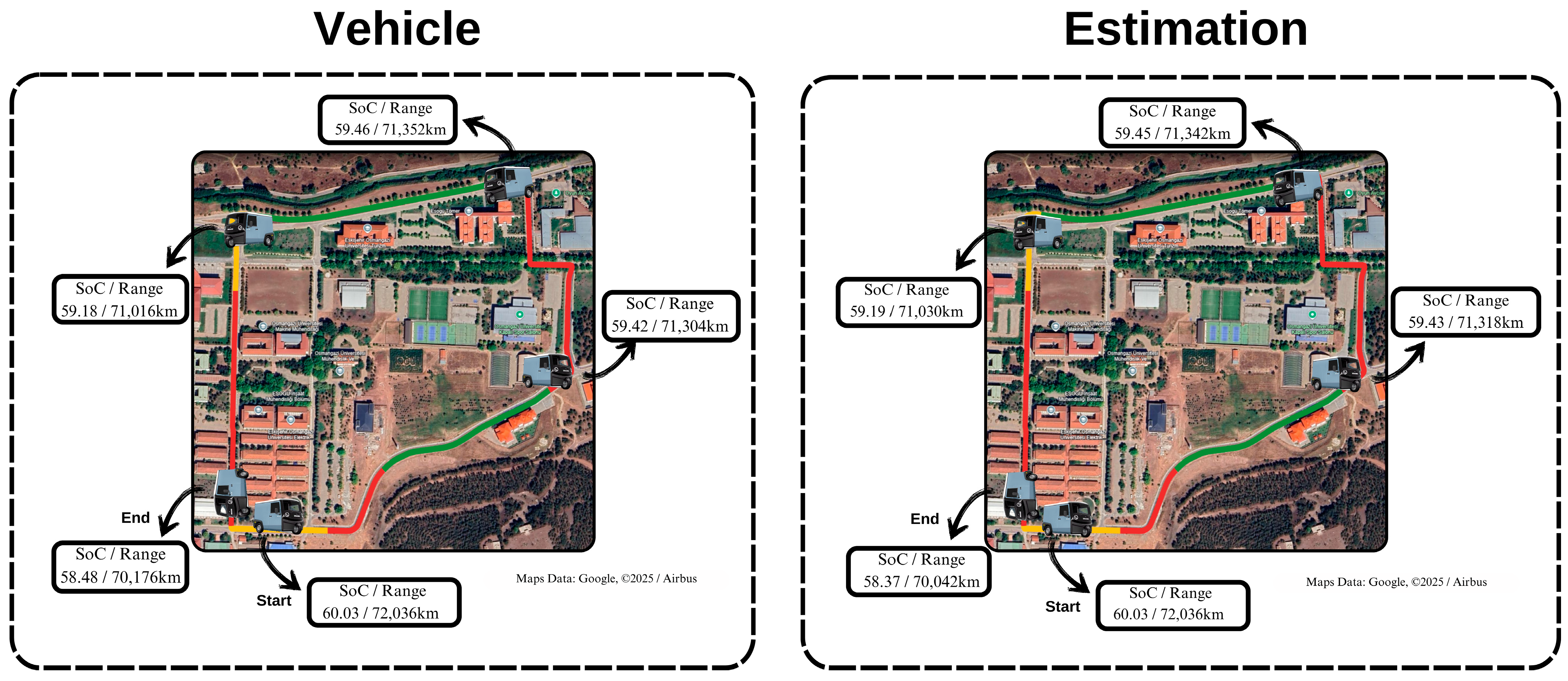
3.3.2. Validation of Range Estimation

The proposed energy consumption-based range estimation method uses various machine learning methods, and a physical energy consumption model [16], which is taken as a reference. This experimental approach allowed us to evaluate to what extent both the traditional physical model and various ML methods accurately modelled difficult driving conditions. This model evaluates the vehicle’s energy consumption step by step, and continuously updates the total energy content. First, the vehicle’s kinetic energy (depending on its speed), potential energy (depending on its altitude), and rotational inertia energy of the internal rotating masses are calculated. This trio represents the vehicle’s current energy status (Equation (3)).

$${\mathrm{E}}_{\mathrm{veh}}\left[\mathrm{k}\right]={\mathrm{E}}_{\mathrm{kin}}\left[\mathrm{k}\right]+{\mathrm{E}}_{\mathrm{pot}}\left[\mathrm{k}\right]+{\mathrm{E}}_{\mathrm{int},\mathrm{rot}}\left[\mathrm{k}\right]$$

(4)

$${\mathrm{E}}_{\mathrm{veh}}\left[\mathrm{k}\right]={\displaystyle \frac{\mathrm{m}}{2}}{\mathrm{v}}^2\left[\mathrm{k}\right]+\mathrm{m}\mathrm{g}\mathrm{h}\left[\mathrm{k}\right]+{\displaystyle \frac{{\mathrm{J}}_{\mathrm{int}}}{2}}{\mathrm{v}}^2\left[\mathrm{k}\right]$$

(5)

The vehicle’s energy status at the next time step is updated based on the energy from the previous step (Equation (6)). Here, energy gain or loss becomes important. If the vehicle is descending a hill or braking, regenerative braking is activated, and can return a certain amount of energy to the battery. However, if the vehicle accelerates, climbs a hill, or struggles with resistance forces, energy is consumed from the battery.

$$\mathsf{\Delta }{\mathrm{E}}_{\mathrm{gain}}\left[\mathrm{k}\right]={\mathrm{E}}_{\mathrm{veh}}\left[\mathrm{k}+1\right]-{\mathrm{E}}_{\mathrm{veh}}\left[\mathrm{k}\right]-\mathsf{\Delta }{\mathrm{E}}_{\mathrm{loss}}\left[\mathrm{k}\right]$$

(6)

Energy losses are caused by various resistances. Air resistance causes energy consumption in direct proportion to the vehicle’s speed and aerodynamic properties. Rolling resistance is another loss item, resulting from the interaction of the tyres with the surface. The curve resistance that occurs when cornering, and fixed consumers integrated into the vehicle (such as headlights, air conditioning), are also among the factors that increase energy consumption. Each resistance item is calculated separately in the model (Equation (7)), then added together and evaluated as the total loss.

$$\mathsf{\Delta }{\mathrm{E}}_{\mathrm{l}\mathrm{o}\mathrm{s}\mathrm{s}}\left[\mathrm{k}\right]=\mathsf{\Delta }{\mathrm{E}}_{\mathrm{a}\mathrm{i}\mathrm{r}}\left[\mathrm{k}\right]+\mathsf{\Delta }{\mathrm{E}}_{\mathrm{r}\mathrm{o}\mathrm{l}\mathrm{l}}\left[\mathrm{k}\right]+\mathsf{\Delta }{\mathrm{E}}_{\mathrm{c}\mathrm{u}\mathrm{r}\mathrm{v}\mathrm{e}}\left[\mathrm{k}\right]+\mathsf{\Delta }{\mathrm{E}}_{\mathrm{c}\mathrm{o}\mathrm{n}\mathrm{s}\mathrm{t}}\left[\mathrm{k}\right]$$

(7)

$$\mathsf{\Delta }{\mathrm{E}}_{\mathrm{air}}\left[\mathrm{k}\right]={\displaystyle \frac{1}{2}}{\mathsf{\rho }}_{\mathrm{air}}{\mathrm{A}}_{\mathrm{veh}}{\mathrm{c}}_{\mathrm{w}}{\mathrm{v}}^2\left[\mathrm{k}\right]|\mathsf{\Delta }\mathrm{s}\left[\mathrm{k}\right]|$$

(8)

$$\mathsf{\Delta }{\mathrm{E}}_{\mathrm{roll}}\left[\mathrm{k}\right]={\mathrm{c}}_{\mathrm{roll}}\mathrm{m}\mathrm{g}|\mathsf{\Delta }\mathrm{s}\left[\mathrm{k}\right]|$$

(9)

$$\mathsf{\Delta }{\mathrm{E}}_{\mathrm{curve}}\left[\mathrm{k}\right]={\mathrm{c}}_{\mathrm{rad}}{\displaystyle \frac{\mathrm{m}{\mathrm{v}}^2\left[\mathrm{k}\right]}{\mathrm{R}\left[\mathrm{k}\right]}}|\mathsf{\Delta }\mathrm{s}\left[\mathrm{k}\right]|$$

(10)

$$\mathsf{\Delta }{\mathrm{E}}_{\mathrm{const}}\left[\mathrm{k}\right]={\mathrm{P}}_{\mathrm{const}}\mathsf{\Delta }\mathrm{t}$$

(11)

In the final step, the amount of energy gained or lost is reflected in the vehicle’s battery level. If the vehicle has gained energy (for example, by regenerative braking downhill), energy is added to the battery according to a certain efficiency rate. If the vehicle has consumed energy, the battery energy is reduced again by a certain drive efficiency factor. Thus, a more realistic estimate is obtained by considering energy fluctuations during driving, physical variables, and efficiency elements.

If ΔE_“gain” [k] > 0 (regeneration), the formula is as follows:

$${\mathrm{E}}_{\mathrm{bat}}\left[\mathrm{k}+1\right]={\mathrm{E}}_{\mathrm{bat}}\left[\mathrm{k}\right]+\mathsf{\Delta }{\mathrm{E}}_{\mathrm{gain}}\left[\mathrm{k}\right]{\mathsf{\eta }}_{\mathrm{recup}}$$

(12)

If ΔE_“gain” [k] < 0 (consumption), the formula is as follows:

$${\mathrm{E}}_{\mathrm{bat}}\left[\mathrm{k}+1\right]={\mathrm{E}}_{\mathrm{bat}}\left[\mathrm{k}\right]+\mathsf{\Delta }{\mathrm{E}}_{\mathrm{gain}}\left[\mathrm{k}\right]{\mathsf{\eta }}_{\mathrm{prop}}$$

(13)

After the definition of the physical model, comprehensive experiments were performed to compare the performance of different ML models. Among the candidate algorithms, five models achieved particularly high accuracy rates, and the analysis is focused on these models. Extra Trees (Extremely Randomized Trees), an ensemble-based method, adds variety to the model with the strategy of determining random split points. It can achieve significant success by speeding up the prediction time in datasets with interactive variables, such as speed, acceleration, and slope [49]. CatBoost is a model based on the gradient boosting method, and is known for its structure that is sensitive to categorical variables and order effects in the data. Each tree focuses on minimizing the error margin of the previous model, and thus follows a training process that carefully considers the order in the data to reduce the risk of overfitting [50]. The Voting Regressor approach is based on training different regression models, such as CatBoost, Extra Trees, and LightGBM, on the same dataset and combining the produced predictions. By using different model structures together, it provides better performance, often exceeding the accuracy that a single model can achieve on its own. XGBoost (eXtreme Gradient Boosting) is a gradient boosting library enriched with optimization principles; it has become popular by providing both high accuracy and short training time in large datasets, thanks to additional mechanisms such as regularization and parallelization [32]. LightGBM is also a gradient boosting-based library which reduces memory usage and increases training speed in large datasets with its leaf-wise growth strategy. It is known for its high success rates, especially in multi-dimensional feature spaces [51]. During the model training process, scikit-learn, CatBoost, LightGBM, and XGBoost libraries are used. The dataset consists of 14698 rows, and 80% of the dataset is separated for training and 20% for testing [52]; in addition, 5-fold cross-validation is applied to measure the general performance of each model consistently. Hyperparameters such as the learning rate, number of trees, and maximum depth are scanned and optimized with Bayesian optimization (Optuna). Optuna is a Python-based and open-source hyperparameter optimization library that systematically scans the parameter range using randomization and Bayesian strategies. In each trial, the parameter selection is evaluated via the R² value and the results are recorded; during this process, the search range is gradually narrowed down using statistical methods such as Tree-structured Parzen Estimators (TPE). Thus, the possible value range of the parameters is effectively scanned, the performance of each trial is measured, and the best-scoring parameter set is determined. With this process, basic parameters, such as the number of estimators, maximum depth, and minimum sample split, are scanned across different intervals; each iteration is evaluated using 5-fold cross-validation. In this way, it the aim for the models to show both high accuracy and strong generalization ability. As a result of experiments with different parameter combinations on different models, it was seen that the Extra Trees model outperforms other models, based on metrics such as the R², MAE, and RMSE.

Finally, based on the information that the vehicle can reach a fully charged battery range of 120 km, and the battery capacity is 15.6 kWh according to the factory data, the process of estimation of the energy consumption during driving and the remaining range estimation at the end of the drive is discussed in detail. First, the energy consumption prediction is determined by the Extra Trees model. Then, how much of a SoC change the energy consumption prediction from the model causes is calculated (Equation (14)).

$${\mathrm{S}\mathrm{o}\mathrm{C}}_{\mathrm{d}\mathrm{i}\mathrm{f}\mathrm{f}\mathrm{e}\mathrm{r}\mathrm{e}\mathrm{n}\mathrm{c}\mathrm{e}}={\displaystyle \frac{{\mathrm{E}}_{\mathrm{e}\mathrm{s}\mathrm{t}\mathrm{i}\mathrm{m}\mathrm{a}\mathrm{t}\mathrm{e}\mathrm{d}}}{\mathrm{B}\mathrm{a}\mathrm{t}\mathrm{t}\mathrm{e}\mathrm{r}\mathrm{y}\mathrm{C}\mathrm{a}\mathrm{p}\mathrm{a}\mathrm{c}\mathrm{i}\mathrm{t}\mathrm{y}\left(\mathrm{w}\mathrm{H}\right)}}\times 100$$

(14)

Then, the SoC difference is subtracted from the initial SoC value, and the remaining estimated SoC value is obtained (Equation (15)).

$${\mathrm{S}\mathrm{o}\mathrm{C}}_{\mathrm{e}\mathrm{s}\mathrm{t}\mathrm{i}\mathrm{m}\mathrm{a}\mathrm{t}\mathrm{e}\mathrm{d}}={\mathrm{S}\mathrm{o}\mathrm{C}}_{\mathrm{s}\mathrm{t}\mathrm{a}\mathrm{r}\mathrm{t}}-{\mathrm{S}\mathrm{o}\mathrm{C}}_{\mathrm{d}\mathrm{i}\mathrm{f}\mathrm{f}\mathrm{e}\mathrm{r}\mathrm{e}\mathrm{n}\mathrm{c}\mathrm{e}}$$

(15)

After determining the estimated SoC, the usable remaining energy is calculated as in Equation (16):

$${\mathrm{E}}_{\mathrm{u}\mathrm{s}\mathrm{a}\mathrm{b}\mathrm{l}\mathrm{e}}=\mathrm{B}\mathrm{a}\mathrm{t}\mathrm{t}\mathrm{e}\mathrm{r}\mathrm{y}\mathrm{C}\mathrm{a}\mathrm{p}\mathrm{a}\mathrm{c}\mathrm{i}\mathrm{t}\mathrm{y}\left(\mathrm{w}\mathrm{H}\right)\times {\displaystyle \frac{{\mathrm{S}\mathrm{o}\mathrm{C}}_{\mathrm{e}\mathrm{s}\mathrm{t}\mathrm{i}\mathrm{m}\mathrm{a}\mathrm{t}\mathrm{e}\mathrm{d}}-{\mathrm{S}\mathrm{o}\mathrm{C}}_{min}}{100}}$$

(16)

where ${\mathrm{S}\mathrm{o}\mathrm{C}}_{min}$ indicates allowed minimum SoC.; here, it is accepted as zero.

Finally, the remaining range is calculated using ${\mathrm{E}}_{\mathrm{u}\mathrm{s}\mathrm{a}\mathrm{b}\mathrm{l}\mathrm{e}}$ and ${\mathrm{E}}_{\mathrm{n}\mathrm{o}\mathrm{n}\mathrm{l}\mathrm{i}\mathrm{n}\mathrm{e}\mathrm{a}\mathrm{r}}$ (Equation (17)):

$${\mathrm{R}\mathrm{a}\mathrm{n}\mathrm{g}\mathrm{e}}_{\mathrm{r}\mathrm{e}\mathrm{m}\mathrm{a}\mathrm{i}\mathrm{n}\mathrm{i}\mathrm{n}\mathrm{g}}={\displaystyle \frac{{\mathrm{E}}_{\mathrm{u}\mathrm{s}\mathrm{a}\mathrm{b}\mathrm{l}\mathrm{e}}}{{\mathrm{E}}_{\mathrm{n}\mathrm{o}\mathrm{n}\mathrm{l}\mathrm{i}\mathrm{n}\mathrm{e}\mathrm{a}\mathrm{r}}}}$$

(17)

where ${\mathrm{E}}_{\mathrm{n}\mathrm{o}\mathrm{n}\mathrm{l}\mathrm{i}\mathrm{n}\mathrm{e}\mathrm{a}\mathrm{r}}$ indicates the average energy consumed per kilometre (Wh/km). The coefficient ${\mathrm{E}}_{\mathrm{n}\mathrm{o}\mathrm{n}\mathrm{l}\mathrm{i}\mathrm{n}\mathrm{e}\mathrm{a}\mathrm{r}}$ is determined using the mean values for each average speed, mass, and slope combination in the dataset.

Using the final SoC value calculated from the energy consumption estimated by the model, the distance that the vehicle can travel during the remaining drive is realistically estimated. This approach reveals both how much of the battery energy is consumed and how much distance the vehicle can travel with the remaining SoC, in an integrated manner. In this whole process, the effects of driving conditions, such as slope, high speed, sudden acceleration, or loaded driving, on energy consumption are revealed more clearly. Extra Trees’ ability to capture multi-dimensional variable interactions, CatBoost’s strategy that considers the ordering feature in the data, LightGBM’s fast training structure, Voting Regressor’s ensemble approach, and Random Forest’s robust decision tree model provide more consistent energy consumption estimates under real driving conditions. This approach provides more realistic predictions in areas such as route optimization and energy management compared to traditional methods, improving both the user experience and supporting accurate infrastructure planning.

4. Experimental Results

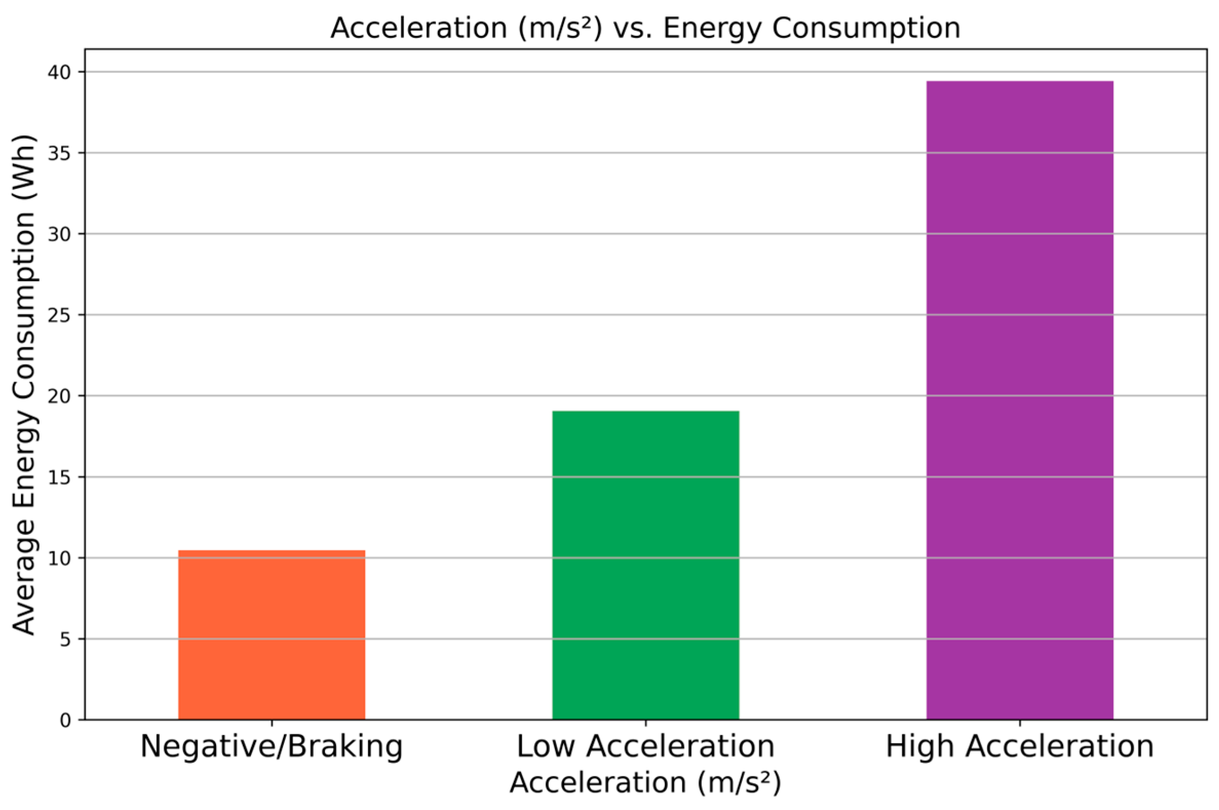
4.1. Analysis of Factors

In this study, different factors affecting the energy consumption of electric vehicles (acceleration, mass, slope, and speed) were analyzed with experimental data, and estimation studies were carried out with machine learning (ML) models, in line with the obtained findings. The numerical reflections of these findings and comprehensive results regarding the performance of the models will be discussed in detail. To understand the interactions between variables more clearly, a heatmap was created, as seen in Figure 4. This map provides the opportunity to visualize how factors such as slope, speed, acceleration, and load affect energy consumption at the level of mutual correlation. Then, variance analyses and correlation studies were performed to determine whether the total energy consumption, speed, slope, and acceleration variables create a statistically significant difference.

As seen in Figure 4, the data reflects the positive or negative linear relationship between the variable pairs. In particular, the correlation of 0.83 between the slope and the total energy consumption observed throughout the segment confirms how much the slope is a determinant for energy needs. Similarly, the correlation value of 0.36 for acceleration supports the fact that high acceleration significantly increases energy consumption. The fact that the speed factor shows a more moderate correlation of 0.11 is also parallel to our previous observations: speed has an effect, but not as strong as that of slope and acceleration. Mass, on the other hand, influences energy consumption with a correlation of 0.20, exhibiting a positive relationship. The effect of temperature is observed to be quite low, with a correlation value of 0.04. These relationships can guide machine learning models in understanding which variables provide more information. Thus, the correlation matrix summarizes the interaction of all these parameters, and constitutes an important reference point for artificial intelligence and machine learning methods in selecting input variables and improving model performance.

Low and negative acceleration values are associated with relatively low energy consumption compared to when the vehicle is in braking or deceleration mode (Figure 5). Especially during negative acceleration (braking), the net consumption level can be reduced in some systems with the contribution of regenerative braking. On the other hand, when the acceleration reaches positive and high values (>1 m/s²), a significant increase in energy consumption is observed. The main reasons for this are the increased torque requirement on the engine for fast acceleration, and the consequent drawing of more electric power. The data confirm that high acceleration significantly increases energy consumption.

With the increase in load, a visible increase in energy consumption is observed. Especially in the loaded state, there is a higher torque requirement, which causes the engine to consume more energy. In addition, the increase in mass increases the friction and rotational resistances, which are important factors affecting the energy consumption of electric vehicles, and thus increase the energy consumption. Therefore, Figure 6 clearly shows that the increase in total mass has a direct effect on energy consumption.

In cases where a negative slope is observed, energy consumption remains at low levels due to the vehicle going downhill, consumption can be further reduced thanks to regenerative braking, and the total energy consumption can even be observed to be below zero, and gains can be dominant (Figure 7). On the other hand, as positive slope values increase, the need for power increases, as the vehicle has to work against gravity, and this situation significantly increases the average energy consumption. Particularly high positive slopes lead to the highest energy consumption values observed, revealing the significant effect of the slope factor on vehicle performance.

Energy consumption remains relatively limited at lower speeds, as air resistance and friction forces are minimal. On the other hand, as speed increases, especially at speeds of 30 kph and above, factors such as aerodynamic drag and rolling resistance grow rapidly, causing the engine to draw more power (Figure 8). The results show that the significant increase in energy consumption is in direct proportion to the increase in speed. Although the trend observed in Figure 8 in electric vehicles for personal use is observed at higher speeds, when the maximum speed of the Musoshi Pop-Up Mini vehicle (50 kph) used in the experiments is considered, speeds of 30 kph and above are considered relatively high. These inferences show that it may be advantageous to stay in the lower or medium speed bands in terms of energy efficiency.

Contrary to expectations, lower energy consumption is observed in cold weather conditions, and higher energy consumption in hot conditions (Figure 9). Technical examinations reveal that the vehicle battery system only has heating pads, and no cooling mechanism. Therefore, the battery exceeding its optimal operating temperature in hot weather causes additional energy consumption, and explains this unusual trend in the data.

When one factor was considered during the analysis, the other factors were kept constant or selected from very small ranges in parts where the data were not sufficient. Also, SHapley Additive exPlanations (SHAP) analyses reveal in detail which variables the model is sensitive to, and how these variables guide the prediction (Figure 10).

First, when the average absolute SHAP values are examined, it is seen that the slope variable makes the highest contribution to the model output. Acceleration is the second most important variable, and it is observed that especially the positive or negative change in acceleration creates a significant change in the results of the model. It is noteworthy that the SHAP value shifts to a positive and higher range with the increase in mass, which shows that the prediction tends to increase in high-weight segments. Although temperature and speed are in the middle ranks in terms of effect size, examination of SHAP distributions shows that these features also play an important role in the model; in particular, the interaction of speed and segment length can affect the model output both positively and negatively. All these findings show that the machine learning model used has strong sensitivity to factors such as slope, acceleration, and mass, and the result validates the determined correlation coefficients. In addition, the Conditional Average Treatment Effect (CATE) distributions estimated for average vehicle speed, slope, average acceleration, total mass, segment length, and average temperature are shown in Figure 11.

The histograms illustrate how changes in these variables affect energy consumption (Wh). Notably, slope (~4.10 Wh) and average acceleration (~4.54 Wh) exhibit the highest positive mean effects, indicating significant increases in energy consumption. By contrast, the mean effects of average vehicle speed, total mass, segment length, and average temperature remain relatively small (under ~0.10 Wh). The results indicate that each factor must be considered together to understand the complex dynamics of vehicle energy consumption, and that holistic consideration of these factors is critical in model development and practical applications.

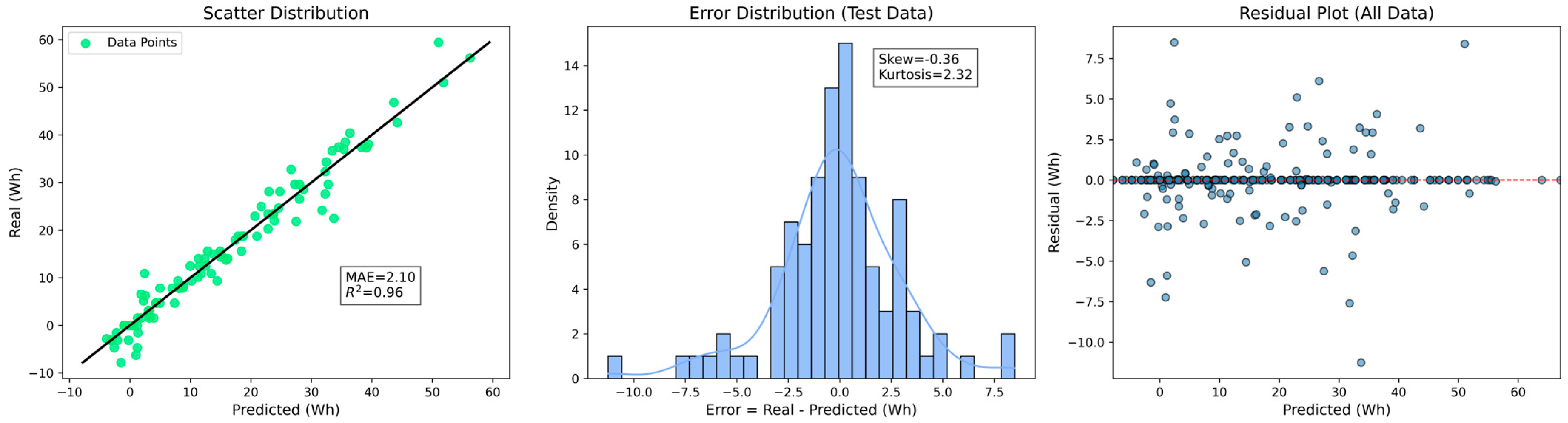
4.2. Estimation of Energy Consumption and Range

Performance comparisons in terms of the R², MAE, and RMSE values of the different machine learning models, as well as their computational times, are listed in

Table 5. Machine learning models performance table.

Model	R2 Score	MAE	RMSE	Training Time (s)	Prediction Time (s)
Extra Trees	0.96	2.1	3.02	0.28	0.03
CatBoost	0.96	2.32	3.17	2.37	0.0
LightGBM	0.95	2.63	3.4	0.06	0.0
Voting Regressor	0.95	2.58	3.46	0.66	0.04
Random Forest	0.94	2.68	3.56	0.52	0.02
Stacking Regressor	0.94	2.74	3.59	3.39	0.02
Gradient Boosting	0.93	2.92	3.81	0.2	0.0
XGBoost	0.92	2.95	4.1	0.22	0.01
Polynomial Regression (Degree 3)	0.89	3.36	4.9	0.01	0.01
Decision Tree	0.87	3.97	5.32	0.01	0.0
AdaBoost	0.87	4.4	5.39	0.17	0.02
Linear Regression	0.81	4.91	6.46	0.01	0.0
Ridge Regression	0.81	4.91	6.46	0.0	0.0
Bayesian Ridge	0.81	4.94	6.47	0.0	0.0
Lasso Regression	0.81	4.94	6.47	0.0	0.0
ElasticNet	0.81	5.0	6.51	0.01	0.0
Huber Regressor	0.81	4.88	6.53	0.08	0.0
Support Vector Regressor (SVR)	0.8	4.6	6.68	0.01	0.01
Theil-Sen Regressor	0.74	4.88	7.59	0.75	0.0
K-Nearest Neighbors (KNN)	0.58	6.91	9.73	0.0	0.0

. It is seen that tree-based ensemble methods capture complex interactions more successfully.

Extra Trees stands out with its high R² score of 0.96 and low error values (MAE = 2.1, RMSE = 3.02). While CatBoost and LightGBM models provide results close to Extra Trees, Voting Regressor and Random Forest also reach satisfactory R² values, at 0.95 and 0.94. On the other hand, methods like XGBoost and Polynomial Regression, and some approaches such as Linear Regression, SVR, and KNN, have higher error metrics. This situation highlights the potential of tree-based ensemble techniques to increase the prediction performance for a problem where many factors are simultaneously active.

Among these tree-based methods, CatBoost stands out with its automatic target coding and gradient-based boosting approach, especially in handling categorical variables. XGBoost and LightGBM also attract attention with their computational efficiency, ability to handle missing data, and high-precision splitting strategies. Extra Trees, on the other hand, captured the complex interactions of the dataset more effectively with the flexible use of random splitting points and tree depth. Low hyperparameter dependency and the ability to capture variable interactions in the data in many random trees allowed it to reduce the risk of overfitting and achieve a high R² value. A scatter plot of the relationship between the predicted energy consumption and the actual consumption is shown in Figure 12.

The fact that the points are mostly close to the diagonal axis shows that Extra Trees makes predictions with high accuracy. The error distribution (prediction−actual) shows that the errors are mostly concentrated in a narrow range, but there is a stretch in the right tail (positive skewness, Skew = 2.32). Despite this, the fact that the prediction errors are generally small confirms that the model fits the actual consumption values.

In order to evaluate the statistical robustness of model performance, both 95% and 98% confidence intervals for R² values were calculated with the bootstrap method. A 20% portion of the dataset, which included a total of 14698 samples, was separated for testing, and bootstrap resampling was applied with 1000 iterations, based on the percentile approach. As a result of this analysis, R² = 0.955 and [0.932, 0.970] for the 95% confidence interval, and R² = 0.955 and [0.929, 0.972] for the 98% confidence interval. The narrow confidence intervals produced by the bootstrap approach show that the high R² value of the model is not random, and its performance is stable.

After estimating the energy consumption, the calculations regarding the remaining range of the vehicle, mentioned in Section 3.3.2, were completed, and then the differences between the range estimates of the vehicle at the beginning of the route and the range estimates at the end of the route were calculated and compared with the actual distance travelled. In

Table 6. Range differences based on trips.

Route	Mass (kg)	Actual Distance (m)	Average Velocity (kph)	Vehicle Range Difference (m)	Estimated Range Difference (m)	PM Range Difference (m)	Actual vs. Vehicle	Actual vs. Predicted	Actual vs. PM
15LC	1195	2047	14.01	1860	1994	1551	9.14%	2.58%	24.22%
15LM	1195	1970	14.32	1716	2019	1587	12.89%	2.48%	19.43%
15UC	870	2047	14.72	1260	1935	1166	38.45%	5.49%	43.06%
15UM	870	1970	14.4	1176	1691	1153	40.30%	14.14%	41.45%
25LC	1220	2047	23.26	2143	2176	2034	4.70%	6.25%	0.62%
25LM	1195	1970	22.39	1956	2033	2166	0.71%	3.18%	9.96%
25UC	870	2047	25.63	1524	1736	1671	25.55%	15.19%	18.37%
25UM	870	1970	25.05	1512	1727	1784	23.25%	12.35%	9.42%
35LC	1220	2047	32.02	2295	2224	2626	12.14%	8.62%	28.28%
35LM	1220	1970	30.65	2364	2178	2828	20.00%	10.56%	43.57%
35UC	870	2047	34.32	1882	1997	2014	8.02%	2.45%	1.63%
35UM	870	1970	33.73	2076	1928	2306	5.38%	2.15%	17.07%

, the average speed, vehicle mass, actual distance, vehicle range, Extra Trees estimations, and physical model calculations are given together for different route scenarios. It is noteworthy that in various routes where the mass varies between 870 and 1220 kg and the speed is measured in the 14–35 km/h band, the average deviation of Extra Trees from the actual range difference is mostly lower than that of the physical model. For example, on route 15LM, the difference between the actual distance and the Extra Trees estimate is approximately 2.48%, while the physical model deviates from the actual distance by 19.43%. Similarly, on the same route, the vehicle range shows a difference of 12.89% compared to the actual value.

All these results show that machine learning methods can better express the multi-dimensional factors (road slope, vehicle mass, driving dynamics, etc.) that play a role in the energy consumption of electric vehicles, compared to physical approaches. However, the physical model also provided reasonable prediction success, especially in low-speed and low-acceleration conditions; nevertheless, the deviation rate increased in difficult driving scenarios where acceleration or mass was high, and the slope of the routes varied greatly.

Figure 13 is designed to compare the vehicle and estimated SoC and range values obtained along short-distance route segments for the urban distribution vehicle. The sections separated from Segment 1 to Segment 13 on the map visualize the effects of factors such as slope, acceleration, speed, and payload on each segment. The SoC and range values measured at the beginning are updated as the segments progress, and are presented side by side with the estimated data at each stage.

Although the machine learning-based model uses only basic factors, such as slope, acceleration, speed, and payload, as inputs, it is striking that the actual and estimated data are quite close. In particular, the similar decrease in SoC and range values along the route proves that the method has sufficient accuracy. Despite the small deviations at the segment end points, the overall picture indicates that the approach shows high performance in battery charge level and possible range estimation. The findings show that if these four factors—slope, acceleration, speed, and payload—are correctly modelled, the battery status and expected range value can be reliably predicted. These results, obtained in urban operations on routes divided into short-distance segments, constitute important evidence that estimates close to real data can be provided. In this way, these results are expected to contribute to the more effective execution of processes such as charging planning and fleet management, especially in urban logistics applications.

5. Conclusions and Future Works

The increasing use of electric vehicles reduces greenhouse gas emissions, reduces dependence on fossil fuels, and increases sustainability in the transportation sector. Range prediction is important, not only for improved performance and customer experience, but also to further the reliability of deployments in various real-world use cases, such as urban deliveries or long-distance travel. In this study, the factors affecting the energy consumption of electric vehicles (acceleration, slope, mass, speed, etc.) were examined in detail, and various machine learning models were trained on the dataset of the proposed experiments, to provide a more accurate estimation of energy consumption and, accordingly, driving range. In particular, tree-based ensemble methods such as Extra Trees, CatBoost, Voting Regressor, XGBoost, and LightGBM provided fast and high-accuracy estimates closest to real consumption values in various driving scenarios. The experiments conducted revealed that the effect on energy consumption becomes more complex when dynamic factors such as speed, acceleration, and slope interact with conditions such as vehicle mass. In addition, comparisons have shown that machine learning approaches produce much more accurate predictions under different driving conditions compared to traditional physical models. The increase in prediction accuracy increases the ease of use and user confidence of electric vehicles, by providing a more accurate calculation of driving range; thus, it contributes to the elimination of range anxiety problems. This study provides insights, by focusing on short-distance segments to optimize the range estimation for electric vehicles, for both theoretical developments and practical applications. The methods presented in the study provide guidance on route optimization and energy consumption reduction for logistics operations.

In future studies, it is the goal to examine the effects of dynamic variables, such as traffic density, waiting times at red lights, and the number of stops and starts, in order to understand energy consumption under real driving conditions, in addition to factors such as battery temperature, ambient temperature, and in-vehicle auxiliary systems (air conditioning, heater, radio, etc.). It is planned to evaluate the effects of regenerative braking and different driving styles on range estimation, due to low speed and frequent braking in heavy traffic conditions. Thus, it is aimed to develop models based on real-time data flows that incorporate dynamically changing conditions along the road, such as traffic density and driver behaviour.

References

1. Coignard, J.; MacDougall, P.; Stadtmueller, F.; Vrettos, E. Will Electric Vehicles Drive Distribution Grid Upgrades?: The Case of California. IEEE Electrif. Mag. 2019, 7, 46–56. [Google Scholar]
2. Qadir, S.A.; Ahmad, F.; Al-Wahedi, A.M.A.B.; Iqbal, A.; Ali, A. Navigating the complex realities of electric vehicle adoption: A comprehensive study of government strategies, policies, and incentives. Energy Strat. Rev. 2024, 53, 101379. [Google Scholar]
3. Ghosh, A. Possibilities and Challenges for the Inclusion of the Electric Vehicle (EV) to Reduce the Carbon Footprint in the Transport Sector: A Review. Energies 2020, 13, 2602. [Google Scholar] [CrossRef]
4. Richardson, D.B. Electric vehicles and the electric grid: A review of modeling approaches, Impacts, and renewable energy integration. Renew. Sustain. Energy Rev. 2013, 19, 247–254. [Google Scholar]
5. Weldon, P.; Morrissey, P.; O’mahony, M. Long-term cost of ownership comparative analysis between electric vehicles and internal combustion engine vehicles. Sustain. Cities Soc. 2018, 39, 578–591. [Google Scholar]
6. Rauh, N.; Franke, T.; Krems, J.F. Understanding the Impact of Electric Vehicle Driving Experience on Range Anxiety. Hum. Factors J. Hum. Factors Ergon. Soc. 2015, 57, 177–187. [Google Scholar]
7. Liu, Q.; Zhang, Z.; Zhang, J. Research on the interaction between energy consumption and power battery life during electric vehicle acceleration. Sci. Rep. 2024, 14, 157. [Google Scholar]
8. Liu, K.; Yamamoto, T.; Morikawa, T. Impact of road gradient on energy consumption of electric vehicles. Transp. Res. Part D Transp. Environ. 2017, 54, 74–81. [Google Scholar]
9. Abousleiman, R.; Rawashdeh, O. Energy Consumption Model of an Electric Vehicle. In Proceedings of the 2015 IEEE Transportation Electrification Conference and Expo (ITEC), Dearborn, MI, USA, 14–17 June 2015; pp. 1–5. [Google Scholar]
10. Brady, J.; O’Mahony, M. Travel to Work in Dublin. The Potential Impacts of Electric Vehicles on Climate Change and Urban Air Quality. Transp. Res. D Transp. Environ. 2011, 16, 188–193. [Google Scholar]
11. Neubauer, J.; Wood, E. The impact of range anxiety and home, workplace, and public charging infrastructure on simulated battery electric vehicle lifetime utility. J. Power Sources 2014, 257, 12–20. [Google Scholar]
12. Vaz, W.; Nandi, A.K.; Landers, R.G.; Koylu, U.O. Electric vehicle range prediction for constant speed trip using multi-objective optimization. J. Power Sources 2015, 275, 435–446. [Google Scholar] [CrossRef]
13. Hong, J.; Park, S.; Chang, N. Accurate Remaining Range Estimation for Electric Vehicles. In Proceedings of the 2016 21st Asia and South Pacific Design Automation Conference (ASP-DAC), Macao, China, 25–28 January 2016; pp. 781–786. [Google Scholar]
14. Sarrafan, K.; Sutanto, D.; Muttaqi, K.M.; Town, G. Accurate range estimation for an electric vehicle including changing environmental conditions and traction system efficiency. IET Electr. Syst. Transp. 2017, 7, 117–124. [Google Scholar] [CrossRef]
15. Helmbrecht, M.; Olaverri-Monreal, C.; Bengler, K.; Vilimek, R.; Keinath, A. How Electric Vehicles Affect Driving Behavioral Patterns. IEEE Intell. Transp. Syst. Mag. 2014, 6, 22–32. [Google Scholar]
16. Kurczveil, T.; López, P.Á.; Schnieder, E. Implementation of an Energy Model and a Charging Infrastructure in SUMO. In Proceedings of the Simulation of Urban Mobility: First International Conference, SUMO 2013, Berlin, Germany, 15–17 May 2013; Revised Selected Papers 1. Springer: Berlin/Heidelberg, Germany, 2014; pp. 33–43. [Google Scholar]
17. Pan, Y.; Fang, W.; Zhang, W. Development of an energy consumption prediction model for battery electric vehicles in real-world driving: A combined approach of short-trip segment division and deep learning. J. Clean. Prod. 2023, 400, 136742. [Google Scholar] [CrossRef]
18. Yao, E.; Yang, Z.; Song, Y.; Zuo, T. Comparison of Electric Vehicle’s Energy Consumption Factors for Different Road Types. Discret. Dyn. Nat. Soc. 2013, 2013, 328757. [Google Scholar] [CrossRef]
19. Zhang, R.; Yao, E. Electric vehicles’ energy consumption estimation with real driving condition data. Transp. Res. Part D Transp. Environ. 2015, 41, 177–187. [Google Scholar] [CrossRef]
20. Amirkhani, A.; Haghanifar, A.; Mosavi, M.R. Electric Vehicles Driving Range and Energy Consumption Investigation: A Comparative Study of Machine Learning Techniques. In Proceedings of the 2019 5th Iranian Conference on Signal Processing and Intelligent Systems (ICSPIS), Shahrood, Iran, 18–19 December 2019; pp. 1–6. [Google Scholar]
21. Fetene, G.M.; Kaplan, S.; Mabit, S.L.; Jensen, A.F.; Prato, C.G. Harnessing big data for estimating the energy consumption and driving range of electric vehicles. Transp. Res. Part D Transp. Environ. 2017, 54, 1–11. [Google Scholar]
22. Lu, L.; Han, X.; Li, J.; Hua, J.; Ouyang, M. A review on the key issues for lithium-ion battery management in electric vehicles. J. Power Sources 2013, 226, 272–288. [Google Scholar] [CrossRef]
23. Tiwary, A.; Mishra, S.; Kumar, U. Electric Vehicle Range Estimation Based on Driving Behaviour Employing Long Short-Term Memory Neural Network. In Proceedings of the 2024 International Symposium on Power Electronics, Electrical Drives, Automation and Motion (SPEEDAM), Ischia, Italy, 19–21 June 2024; pp. 551–555. [Google Scholar]
24. Huang, H.; Li, B.; Wang, Y.; Zhang, Z.; He, H. Analysis of Factors Influencing Energy Consumption of Electric Vehicles: Statistical, Predictive, and Causal Perspectives. Appl. Energy 2024, 375, 124110. [Google Scholar]
25. Gurusamy, A.; Bokdia, A.; Kumar, H.; Ashok, B.; Gunavathi, C. Appositeness of automated machine learning libraries on prediction of energy consumption for electric two-wheelers based on micro-trip approach. Energy 2025, 320, 135199. [Google Scholar] [CrossRef]
26. Yılmaz, M.; Çinar, E.; Yazıcı, A. A Transformer-Based Model for State of Charge Estimation of Electrical Vehicle Batteries. IEEE Access 2025, 13, 33035–33048. [Google Scholar]
27. Lee, C.-H.; Wu, C.-H. A Novel Big Data Modeling Method for Improving Driving Range Estimation of EVs. IEEE Access 2015, 3, 1980–1993. [Google Scholar] [CrossRef]
28. Sarrafan, K.; Muttaqi, K.M.; Sutanto, D.; Town, G.E. A Real-Time Range Indicator for EVs Using Web-Based Environmental Data and Sensorless Estimation of Regenerative Braking Power. IEEE Trans. Veh. Technol. 2018, 67, 4743–4756. [Google Scholar]
29. Çeven, S.; Albayrak, A.; Bayır, R. Real-time range estimation in electric vehicles using fuzzy logic classifier. Comput. Electr. Eng. 2020, 83, 106577. [Google Scholar]
30. Rhode, S.; Van Vaerenbergh, S.; Pfriem, M. Power prediction for electric vehicles using online machine learning. Eng. Appl. Artif. Intell. 2020, 87, 103278. [Google Scholar]
31. Zhao, L.; Yao, W.; Wang, Y.; Hu, J. Machine Learning-Based Method for Remaining Range Prediction of Electric Vehicles. IEEE Access 2020, 8, 212423–212441. [Google Scholar] [CrossRef]
32. Chen, T.; Guestrin, C. Xgboost: A Scalable Tree Boosting System. In Proceedings of the 22nd ACM SIGKDD International Conference on Knowledge Discovery and Data Mining, San Francisco, CA, USA, 13–17 August 2016; pp. 785–794. [Google Scholar]
33. Zamee, M.A.; Han, D.; Cha, H.; Won, D. Self-supervised online learning algorithm for electric vehicle charging station demand and event prediction. J. Energy Storage 2023, 71, 108189. [Google Scholar]
34. Dong, Z.; Ji, X.; Wang, J.; Gu, Y.; Wang, J.; Qi, D. ICNCS: Internal Cascaded Neuromorphic Computing System for Fast Electric Vehicle State-of-Charge Estimation. IEEE Trans. Consum. Electron. 2023, 70, 4311–4320. [Google Scholar]
35. Selvaraj, V.; Vairavasundaram, I. A Bayesian optimized machine learning approach for accurate state of charge estimation of lithium ion batteries used for electric vehicle application. J. Energy Storage 2024, 86, 111321. [Google Scholar] [CrossRef]
36. Mishra, D.P.; Kumar, P.; Rai, P.; Kumar, A.; Salkuti, S.R. Exploratory data analysis for electric vehicle driving range prediction: Insights and evaluation. Int. J. Appl. Power Eng. 2024, 13, 474–482. [Google Scholar] [CrossRef]
37. Topić, J.; Škugor, B.; Deur, J. Neural Network-Based Modeling of Electric Vehicle Energy Demand and All Electric Range. Energies 2019, 12, 1396. [Google Scholar] [CrossRef]
38. Varga, B.O.; Sagoian, A.; Mariasiu, F. Prediction of Electric Vehicle Range: A Comprehensive Review of Current Issues and Challenges. Energies 2019, 12, 946. [Google Scholar] [CrossRef]
39. López, F.C.; Fernández, R.Á. Predictive model for energy consumption of battery electric vehicle with consideration of self-uncertainty route factors. J. Clean. Prod. 2020, 276, 124188. [Google Scholar]
40. Miri, I.; Fotouhi, A.; Ewin, N. Electric vehicle energy consumption modelling and estimation—A case study. Int. J. Energy Res. 2021, 45, 501–520. [Google Scholar]
41. Ullah, I.; Liu, K.; Yamamoto, T.; Zahid, M.; Jamal, A. Electric vehicle energy consumption prediction using stacked generalization: An ensemble learning approach. Int. J. Green Energy 2021, 18, 896–909. [Google Scholar]
42. Kocaarslan, I.; Zehir, M.A.; Uzun, E.; Uzun, E.C.; Korkmaz, M.E.; Cakiroglu, Y. High-Fidelity Electric Vehicle Energy Consumption Modelling and Investigation of Factors in Driving on Energy Consumption. In Proceedings of the 2022 4th Global Power, Energy and Communication Conference (GPECOM), Cappadocia, Turkey, 14–17 June 2022; pp. 227–231. [Google Scholar]
43. Sun, L.; An, X.; Geng, P.; Geng, Y. Energy Consumption Evaluation of an Electric Vehicle Under Different Driving Conditions. In Proceedings of the 2023 7th International Conference on Power and Energy Engineering (ICPEE), Chengdu, China, 22–24 December 2023; pp. 229–234. [Google Scholar]
44. Achariyaviriya, W.; Wongsapai, W.; Janpoom, K.; Katongtung, T.; Mona, Y.; Tippayawong, N.; Suttakul, P. Estimating Energy Consumption of Battery Electric Vehicles Using Vehicle Sensor Data and Machine Learning Approaches. Energies 2023, 16, 6351. [Google Scholar] [CrossRef]
45. Yılmaz, H.; Yagmahan, B. Electric vehicle energy consumption prediction for unknown route types using deep neural networks by combining static and dynamic data. Appl. Soft Comput. 2024, 167, 112336. [Google Scholar]
46. Wang, L.; Yang, Y.; Zhang, K.; Liu, Y.; Zhu, J.; Dang, D. Enhancing Electric Vehicle Energy Consumption Prediction: Integrating Elevation into Machine Learning Model. In Proceedings of the 2024 IEEE Intelligent Vehicles Symposium (IV), Jeju Island, Republic of Korea, 2–5 June 2024; pp. 2936–2941. [Google Scholar]
47. Gioldasis, C.; Christoforou, Z.; Katsiadrami, A. Usage factors influencing e-scooter energy consumption: An empirical investigation. J. Clean. Prod. 2024, 452, 142165. [Google Scholar]
48. Kozłowski, E.; Wiśniowski, P.; Gis, M.; Zimakowska-Laskowska, M.; Borucka, A. Vehicle Acceleration and Speed as Factors Determining Energy Consumption in Electric Vehicles. Energies 2024, 17, 4051. [Google Scholar] [CrossRef]
49. Geurts, P.; Ernst, D.; Wehenkel, L. Extremely Randomized Trees. Mach. Learn. 2006, 63, 3–42. [Google Scholar]
50. Prokhorenkova, L.; Gusev, G.; Vorobev, A.; Dorogush, A.V.; Gulin, A. CatBoost: Unbiased Boosting with Categorical Features. arXiv 2017, arXiv:1706.09516. [Google Scholar]
51. Ke, G.; Meng, Q.; Finley, T.; Wang, T.; Chen, W.; Ma, W.; Ye, Q.; Liu, T.-Y. Lightgbm: A Highly Efficient Gradient Boosting Decision Tree. In Proceedings of the 31st International Conference on Neural Information Processing Systems, Long Beach, CA, USA, 4–9 December 2017. [Google Scholar]
52. ESOGU-ML5EV Dataset (v1.0.0). Zenodo. Available online: https://doi.org/10.5281/zenodo.14912892 (accessed on 10 January 2025).
Figure 1. The flow diagram of the proposed method.
Sustainability 17 03488 g001
Figure 2. Planned route.
Sustainability 17 03488 g002
Figure 3. Road segments.
Sustainability 17 03488 g003
Figure 4. Heatmap of used features with Pearson correlation coefficients.
Sustainability 17 03488 g004
Figure 5. Relationship between average acceleration and average energy consumption.
Sustainability 17 03488 g005
Figure 6. Relationship between total mass and average energy consumption.
Sustainability 17 03488 g006
Figure 7. Relationship between slope and average energy consumption.
Sustainability 17 03488 g007
Figure 8. Relationship between average vehicle speed and average energy consumption.
Sustainability 17 03488 g008
Figure 9. Relationship between weather and average energy consumption.
Sustainability 17 03488 g009
Figure 10. SHapley Additive exPlanations.
Sustainability 17 03488 g010
Figure 11. CATE distributions.
Sustainability 17 03488 g011
Figure 12. Predicted energy consumption.
Sustainability 17 03488 g012
Figure 13. Visualization of actual and estimated ranges.
Sustainability 17 03488 g013