Revealing Black Stains on the Surface of Stone Artifacts from Material Properties to Environmental Sustainability: The Case of Xianling Tomb, China

Abstract

Around the world, a large number of stone artifacts have been exposed to air for long periods of time, showing multiple types of deterioration that have attracted widespread attention. Among them, there is an often overlooked deterioration of stone artifacts, i.e., black stains on the surface of the calcareous stone, which are tightly bonded to the substrate as a result of the long-term deposition of air pollution. However, due to the current lack of a clear understanding of the black stains, people often tend to use the wrong cleaning and conservation methods, which is not conducive to sustainable conservation. Therefore, there is an urgent need to comprehensively recognize the black stains in terms of material properties and environmental sustainability to guide scientific sustainable conservation methods. To this end, in this paper, we take the black stains observed on marble buildings in the Xianling Tomb, China, as an example, and for the first time, we aim to create a comprehensive understanding of black deposition from the aspects of material properties and environmental characteristics. Multi-analytical approaches, including polarized light microscopy, X-ray fluorescence (XRF), and scanning electron microscopy with energy dispersive X-ray spectrometry (SEM-EDS), were employed to discern the differences between the substrate and black stains. The results revealed that the formation of black stains was attributed to prolonged exposure to various air pollutants (PM, SO₂, NO₂, CO, and O₃). Subsequently, observational data from 2015 to 2023 were utilized to investigate the temporal evolution of local air pollutants and their coupled resonances. Multi-scale variations (annual, seasonal, monthly, weekly, and daily) of pollutant concentration sequences were identified, which helps us to have a clearer perception and to proactively control air pollutants in the region from different cycles. In addition, wavelet coherence (WTC) demonstrated significant time-scale dependency in correlation with air pollutants, which provides effective data support for the coordinated control of air pollutants. This study reveals the mechanism of black stain deterioration on stone artifact surfaces, provides data support for the control and prediction of air pollutants oriented to the sustainable conservation of stone artifacts, and provides a novel and comprehensive approach to the scientific knowledge and sustainable conservation of stone artifacts.

1. Introduction

Air pollutants play a crucial role in material deterioration, thereby significantly impacting buildings with historical and artistic value [1,2]. A number of physicochemical processes take place on the surfaces of historic buildings, developing discolorations related to the type of the environmental attacks and the type of material exposed [3,4]. In a polluted environment, the surfaces of calcareous historic buildings frequently exhibit black stains [5,6]. Compounds derived from air pollutions undergo a transformation and give rise to new minerals, which then reach the surfaces of buildings and interact with their substrates, often resulting in structural degradation and color changes [7,8]. The abundant presence of carbonate matrices (i.e., calcite, dolomite) in calcareous stones makes them more susceptible to damage from air pollutants [1,9].

In the context of rapid urban and industrial development worldwide, surface blackening on carbonate buildings has become increasingly prevalent [5,10]. The increase of pollutant types and their synergistic effects has led to a growing complexity in the causes of black stain formation [5,11]. Over the past century, sulfur dioxide (SO₂) from fossil fuel combustion has been identified as the primary driver of calcareous stone deterioration [12,13]. When SO₂ deposits onto calcium carbonate (CaCO₃), the stone surface transforms into calcium sulfate hemihydrate (CaSO₃•0.5H₂O) and gypsum (CaSO₄•2H₂O) [14,15,16]. While gypsum, being soluble in water, is typically washed away, black stains (gypsum encrusted with embedded ash particles) remain on carbonate surfaces [17,18,19]. It is noteworthy that SO₂ emissions have gradually decreased due to improvements in industrial practices and the adoption of low-sulfur fuels [20]. Conversely, the ongoing demand for transportation has led to a continuous increase in pollutants from mobile sources, such as ozone (O₃), nitrogen oxides (NO_x), carbon monoxide (CO), and particulate matter (PM) rich in organic compounds [20,21]. Consequently, the formation of black stains has shifted from being predominantly influenced by SO₂ to the combined effects of various pollutants including PM [8,22,23], NO_X [24,25], and O₃ [26], and the effects of different air pollutants have gradually manifested themselves in an intertwined pattern. For example, SO_x and NO_x can form sulfates and nitrates through chemical processes, which attach to existing PM and accumulate into larger particles, accelerating their deposition and leading to the occurrence of black stains [27,28]. Therefore, the formation of black stains on calcareous stone surfaces often depends on the type and concentration of air pollutants [29,30], posing a challenging issue worthy of further investigation.

Effectively controlling and predicting multiple pollutant concentrations will contribute to addressing the challenges in the preservation of widespread calcareous buildings, necessitating a scientific understanding of their temporal evolution. However, the variability of air pollutant sequences in the time-frequency domain is influenced by complex formation mechanisms (i.e., meteorological conditions, topography, emissions from natural and human activities), and they tend to exhibit multiscale, non-stationary, and localized characteristics, increasing the difficulty of their evaluation [31,32,33,34]. Moreover, air pollutants are interrelated, and considering the synergistic effects among them is essential for more effective control and prediction. However, due to the complex physical and chemical transformation mechanisms or similar sources [35,36], the correlations between air pollutants are intricate and varied, often accompanied by nonlinear dynamics and multiscale effects [37,38]. Therefore, to effectively address air pollutions under the context of heritage conservation, it is imperative to extensively investigate the multi-timescale variations in pollutant concentrations and their coupled resonances using more suitable analytical methods.

In recent years, China’s atmospheric monitoring capabilities have improved, providing a data foundation for effectively managing the complex changes in air pollutants. Since January 2013, the Ministry of Environmental Protection has started releasing data on the concentrations of six standard air pollutants (PM_2.5, PM₁₀, SO₂, NO₂, CO, and O₃) in major cities [39,40]. Many researchers have employed the released data to study the spatiotemporal variations of air pollutant concentrations and their correlations at regional, provincial, and urban scales [39,40,41]. It has been found that traditional time-series analysis methods and correlation analyses have limitations and cannot fully reveal the complex evolution of pollutant concentration sequences [42,43]. They fail to distinguish variations at different time scales and are not applicable to non-monotonic and nonlinear relationships [44]. However, the above limitations are effectively addressed by the wavelet transform, which utilizes wavelet basis functions to decompose time series into temporal and frequency components, helping to elucidate dominant patterns of evolution and how these patterns change over time [45]. Consequently, spectrum analysis methods based on wavelet transforms have increasingly found powerful tools that can be used to reveal the multi-scale variations in air pollutant signals [45,46].

The Xianling Tomb, located in Jingmen city, Hubei Province, is a World Heritage site with extensive black stains on outdoor calcareous buildings, severely damaging the historical value. However, research on the Xianling Tomb primarily focuses on architectural and artistic features, with studies on regional air pollutants mainly concentrating on the provincial capital city, Wuhan [47,48]. In fact, many studies on air pollutant evolution in Chinese urban areas have focused on first- and second-tier cities (i.e., Beijing [27,49], Shanghai [46], and Wuhan [47]), as research aims to improve living environments rather than heritage preservation [50,51]. However, Jingmen city has a lower population density and economic level, placing it in the fourth-tier city category in China. As of 2023, Jingmen city has a permanent population of 2.55 million and a GDP of 227.23 billion, whereas cities like Wuhan have a much higher population (13.65 million) and GDP (2.00 trillion). Generally speaking, the evolution patterns of air pollutants are closely related to the industrial level, population size, and traffic structure of cities [20,42], implying that pollution control experiences from large cities may not apply to smaller and medium-sized cities. Therefore, to formulate more precise heritage conservation strategies, it is crucial to explore the regional characteristics of air pollutant evolution in Jingmen city.

This study comprehensively evaluated the characteristics of widespread black stains on the surfaces of carbonate buildings in the Xianling Tomb. By comparing the microstructure and chemical composition of the substrate and black stains, the formation mechanism of black stains and synergistic destructive effects of various air pollutants were clarified. For precise and effective heritage preservation, the temporal evolution of air pollutants (PM_2.5, PM₁₀, SO₂, NO₂, CO, and O₃) and the coupled resonances among them were investigated. Multi-scale variations (annual, seasonal, monthly, weekly, and daily) of pollutant concentration sequences were identified. Various methods, including the Mann–Kendall test, discrete wavelet decomposition, and continuous wavelet transform, were employed to enhance the understanding of trends, mutations, and periodicities in sequences. Further, wavelet coherence was used to quantify multiscale correlations of various air pollutants in the time-frequency domain, capturing dominant periods, coherent distributions, and time-lag characteristics. These findings supported the prediction and control of air pollutants around the Xianling Tomb and guided conserving calcareous architectural heritage in medium and small-sized cities across China.

2. Materials and Methods

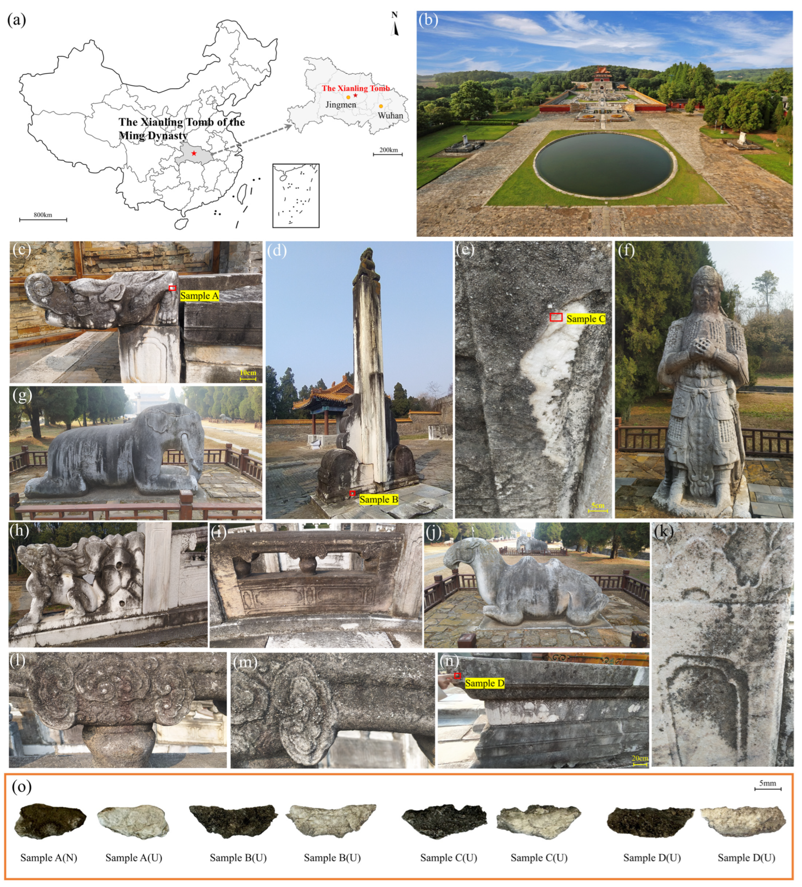
2.1. Study Area

Located in Jingmen city, Hubei province, the Xianling Tomb spans from 31°12′2″ to 31°13′00″ N latitude and from 112°37′50″ to 112°38′09″ E longitude (Figure 1). As one of only four World Heritage Sites in Hubei province, the Xianling Tomb stands as an exemplary imperial tomb in China, boasting significant historical and cultural value. Constructed in 1519, it covers a total area of 183.15 hectares, with the tomb area spanning 52 hectares. Designated as part of the “Ming and Qing Imperial Tombs”, the Xianling Tomb was inscribed in the World Heritage List in 2000. The mausoleum area preserves numerous precious stone artifacts, including stone pedestals, stone-carved railings, and stone statues. The stones used can be distinctly classified into two colors: white and bluish-white. The white stones display a noticeable luster (Figure 1c,d,h,i,l,m), while the bluish-white stones possess a darker, bluish hue (Figure 1e,f,g,j,k,n). Although historical records suggest that the stone components of the Xianling Tomb were mainly made of marble, the specific type remains to be conclusively determined. Over the years, the majority of stone components exposed outdoors have been adversely affected by various environmental factors, resulting in poor overall preservation. Black stains adhere firmly to the surface of numerous artifacts, causing the gradual loss of detail in the reliefs (Figure 1c–n). These black stains are prevalent on almost all stone components, causing extensive damage to the cultural heritage value.

2.2. Sample Description

Four stone fragments with surface black stains were collected from different locations within the Xianling Tomb, labeled as A, B, C, and D. Sample A and B were collected from white stones (Figure 1c,d), and sample C and D were collected from bluish-white stones (Figure 1e,n). The four samples could be divided into the following two parts: inner (substrate) labeled as A(U), B(U), C(U), and D(U), and outer (black stains) labeled as A(N), B(N), C(N), and D(N) (Figure 1o). The black stains (N-series) exhibited thin thickness and showed good adhesion to the substrate, making them difficult to remove. All samples mainly originated from stone fragments about to detach; hence, some parts of the substrate (e.g., Sample D(N)) also exhibited slight contamination. In our study, we conducted a detailed surface analysis, and our results indicate that microorganism presence was minimal or absent on the examined artifacts. The primary causes of degradation observed in our research were related to environmental factors, particularly prolonged exposure to air pollutants, humidity variations, and temperature fluctuations, which have led to chemical and physical changes in the stone material.

2.3. Stone Material Characterization Methods

For a complete characterization of stone substrates and alteration products, the following analytical techniques were employed. Thin sections of unaltered stones were prepared for mineralogical and petrographic studies under a transmitted light polarizing optical microscope (LABORLUX 12POL, LEITZ, Oberkochen, Germany) with special reference to different types of marble. The major element compositions of samples were determined using an X-ray fluorescence spectrometer (XRF, Axios MAX, Almelo, The Netherlands). A comparison of microstructure and chemical elements of the substrate and black stains was studied by a CLARA GMH scanning electron microscopy (SEM, TESCAN, Brno, Czech Republic) equipped with Ultim Extreme energy dispersive X-ray (EDS, TESCAN, Brno, Czech Republic). A gold coating was employed on the samples before SEM imaging to improve imaging quality.

2.4. Data Source and Data Processing Methods

To investigate the current status and temporal evolution of ambient air pollution in the Xianling Tomb, monitoring data of major pollutant concentrations (PM_2.5, PM₁₀, SO₂, NO₂, CO, and O₃) were counted from January 2015 to December 2023. The data were collected from a single station in Jingmen city and sourced from the National Urban Air Quality Real-time Monitoring Platform (https://www.cnemc.cn/, accessed on 1 February 2024). In analyzing air pollutant monitoring data, monthly averages were calculated from daily measurements, and then annual averages were derived accordingly. Linear regression and the Mann–Kendall (MK) test were used to identify significant trends in the time series [52,53]. Mean mutations were also determined using the MK test [54]. Further, wavelet analysis was employed to assess the complexity of air pollutant sequences by capturing local variations across the time-frequency domain [42,46]. Specifically, Morlet wavelets were used to generate real part wavelet coefficients and wavelet variances to determine the primary period(s) [45,46]. Discrete wavelet decomposition was utilized to obtain rate mutations [42,44]. Using wavelet coherence (WTC) [53,55], on the basis of the Pearson and Spearman Correlation [56,57], the coupled oscillations of multiple air pollutants on different time scales were further elucidated, revealing the coherent distributions and time-lag characteristics [37]. In addition, comparisons were made with the Chinese Ambient Air Quality Standards Grade II (CAAQS) (GB3095-2012) (Table S1) to assess the degree of the improvement of air pollutants [39].

3. Characterization of the Black Stains

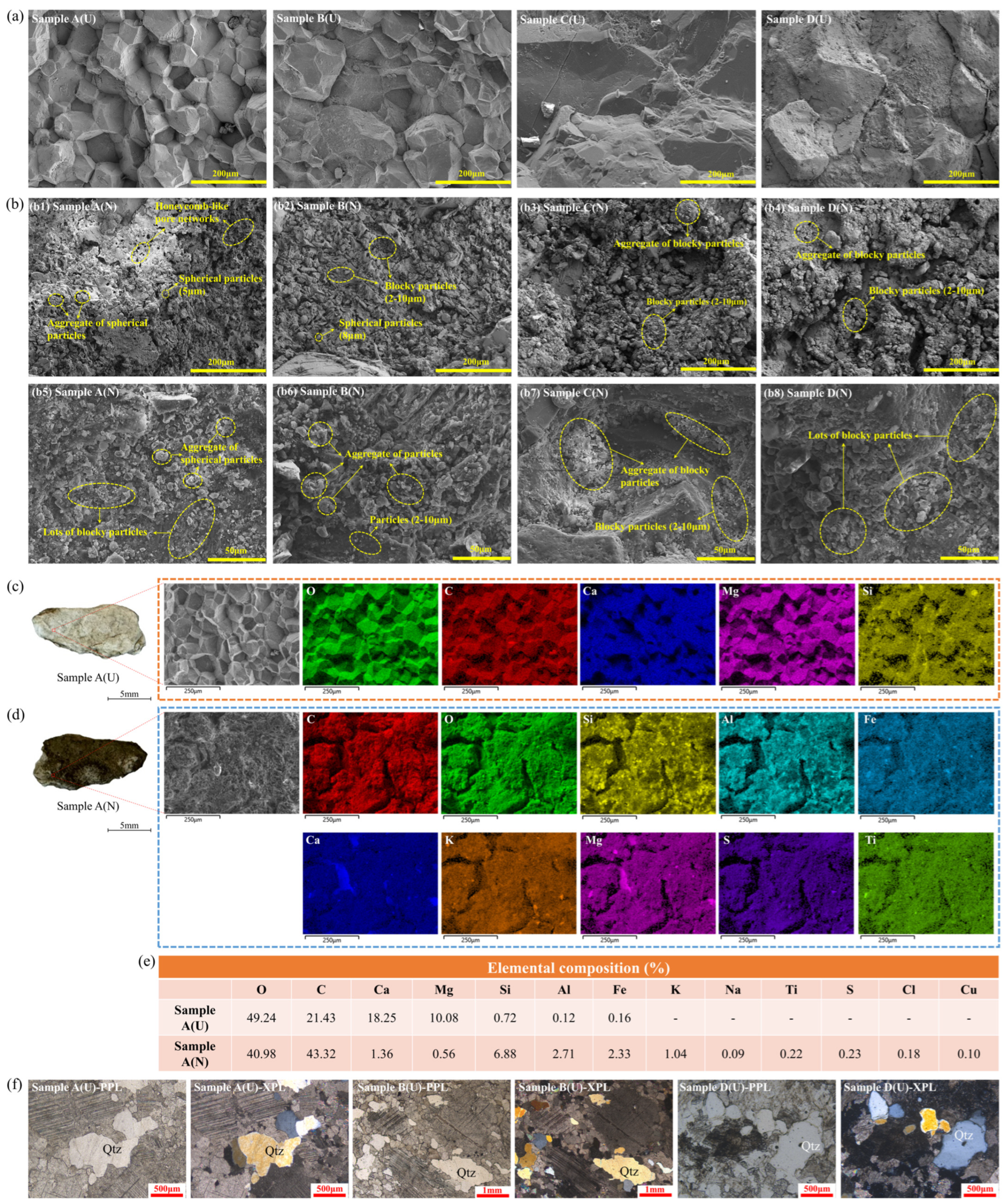
3.1. The Stone Substrate

The petrographic investigation revealed that the white stone fragments (samples A and B) predominantly consisted of dolomite (55% and 90%, respectively), calcite (40% and 3%, respectively), quartz (3% and 5%, respectively), and minor proportions of clay minerals (both 2%) (Figure 2a–f). In contrast, the bluish-white stone samples were primarily composed of calcite (both 75%), dolomite (both 15%), and minor amounts of clay minerals (5% and 4%, respectively) (Figure 2g–l). Additionally, sample C contained trace amounts of tremolite (4%) and scapolite (1%), while sample D contained trace amounts of quartz (5%) and muscovite (1%) (Figure 2g–i). These findings indicated that both the white and bluish-white stone samples fell within the marble category, with the primary distinction lying in the proportions of dolomite (CaMg(CO₃)₂) and calcite (CaCO₃). According to extensive prior research [5,58,59], samples A and B belonged to dolomitic marble, while samples C and D belonged to calcitic marble, commonly found as an associated ore of dolomitic marble [58]. The XRF analysis further confirmed the very low Mg/Ca ratio of calcareous marbles (less than 0.05 [58,59]), with samples A and B (0.38 and 0.43, respectively) having lower Mg/Ca ratios compared to samples C and D (both 0.04) (Table S2).

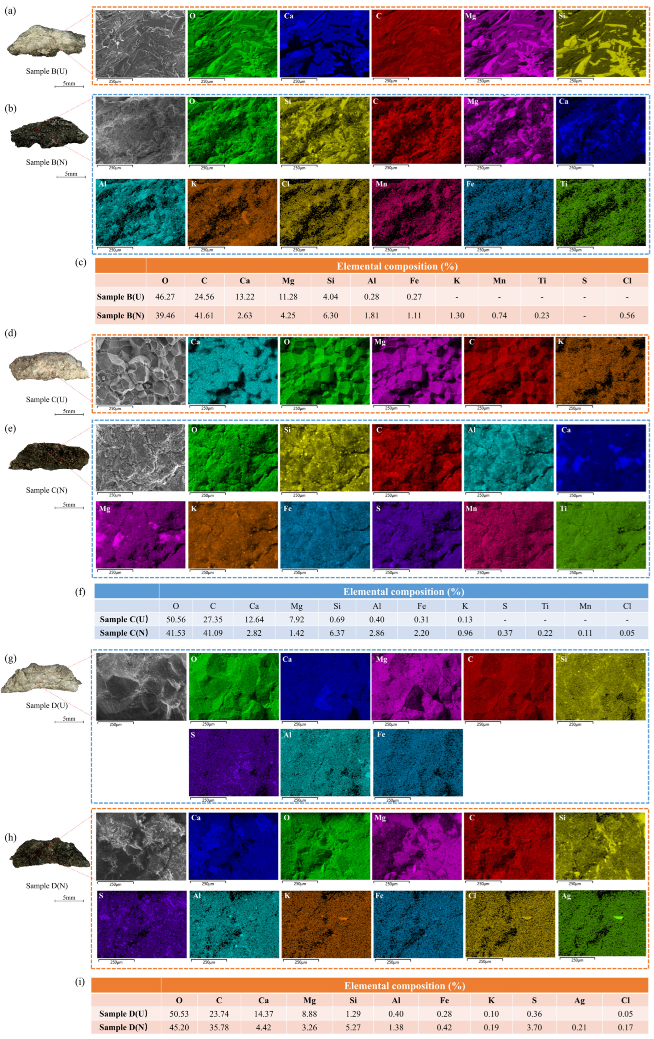
3.2. The Black Stains

Differences in the microstructure of the substrate and black stains were observed. In the U series samples, mineral grains exhibited tight cohesion with relatively smooth surfaces, forming a framework primarily composed of equiaxed minerals embedded with each other, with only a few discernible interlayer cracks (Figure 3a). However, the surface morphology of the N series samples markedly differed from that of the U series. In samples A(N), B(N), C(N), and D(N), the previously cohesive structures were almost entirely obscured, with numerous spherical particles (~2–10 μm), blocky particles (~2–10 μm), and flocculent particles (particle aggregates) adhering to the surface (Figure 3b). The cohesion between particles was weak, resulting in various pores and cracks, with some samples displaying honeycomb-like pore networks (Figure 3(b1)). The complete coverage of the black stains fundamentally altered the microstructure of the substrate, transforming the original face-to-face connection into a point-to-surface connection and changing the initially dense and uniform structure into a loose, porous, irregular structure.

Furthermore, the EDS results showed that the substrate of the four samples (U series) displayed high enrichment of C, O, Ca, and Mg, indicative of calcite and dolomite as the principal mineral constituents (Figure 3c and Figure 4). However, the black stains (N series) showed a marked reduction in Ca and Mg, with only slight enrichment in exposed substrate areas (Figure 3d and Figure 4b,e,h). Notably, a conspicuous elevation in C content became the hallmark of the black stains, suggesting the accumulation of carbonaceous particles. This finding was consistent with previous studies where carbonaceous components (EC and OC) in PM were considered the primary contributors to increased C on black stains [7,23]. Additionally, the relative enrichment of metallic elements was consistently observed in the black stains compared to the substrate (Figure 3d and Figure 4). Sample A(N) exhibited the presence of Fe, Al, Ti, Mn, K, and Cu, which were less prevalent in the substrate (Figure 3c,d). This difference persisted across the other three sample groups (Figure 4). The analogous enrichment of metallic elements was primarily attributed to the deposition of metal substances from atmospheric particulate on the marble surface [11,60].

Moreover, samples A, C, and D displayed a significant rise in Si content on the blackened surfaces (Figure 3e and Figure 4f,i). Petrographic analysis indicated trace amounts of quartz (3–5%) in the substrate, unevenly distributed with larger grain sizes (up to 1.6 mm), with some forming aggregates and further augmenting the grain size (Figure 3f). In contrast, the Si-rich grains on the black stains were primarily distributed uniformly in point-like forms, with most being smaller than 10 μm, probably representing finely ground and rounded quartz particles. The micrometer-scale, point-like distribution of Si elements in black stains indicated that they were late-stage degradation products. Indeed, quartz was commonly found in PM₁₀ [5,61]. Studies by C. Samara et al. [5] and M.F. La Russa et al. [7] also found Si enrichment on the blackened surfaces of marble, which were attributed to atmospheric particulate deposition. Furthermore, S elements were detected on the surface of certain black stains (samples A(N), C(N), D(N)) (Figure 3d and Figure 4), indicating potential sulphation. It is generally believed that S elements in outdoor marble structures originate from atmospheric SO₂ [8,14]. In addition, particles containing K and Cl elements were observed on samples A(N), B(N), and D(N) (Figure 3e and Figure 4b,h), possibly linked to sylvite (KCl) produced during biomass combustion [5,62].

The construction stones of the Xianling Tomb included dolomitic marble and calcite marble, both categorized as calcareous stone. SEM-EDS analysis of the substrate and black stains across the four sets of samples yielded consistent results. The black stains could be regarded as passive samplers of atmospheric pollutants, influenced by a combination of various air pollutants over extended periods. Enrichment of the C element, the presence of metallic elements (Fe, Al, Ti, Mn, K, Cu, Ag), and the occurrence of Si and S underscore the roles played by PM, SO₂, and CO. Moreover, SO₂ and NO₂ served as significant precursors of PM [37,63], while NO₂ and O₃ played crucial catalytic and accelerating roles in sulfation and deposition processes [8,60]. These findings emphasize the importance of exploring the temporal evolution of air pollutants in Jingmen, the location of the Xianling Tomb, with the objective of protecting cultural heritage. Analyzing trends and cycles of air pollutant sequences and deciphering the temporal distribution of high concentrations and concentration mutations are crucial for precise control. Furthermore, understanding the synergistic destructive effects of multiple pollutants requires a clear comprehension of their multiscale resonances across all time-frequency domains to provide a scientific foundation for coordinated control measures.

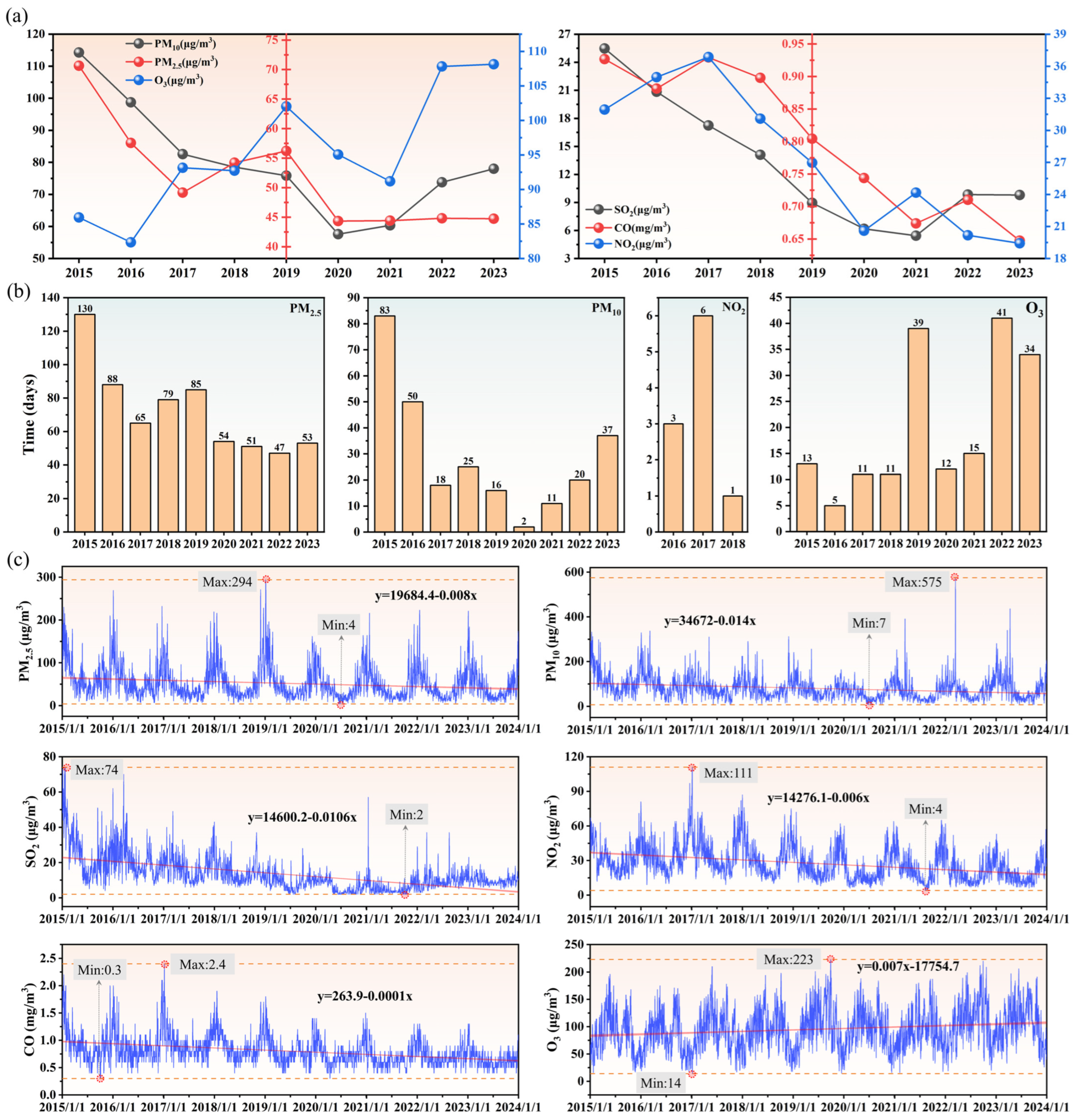
4. Temporal Evolution of Air Pollutant Concentrations

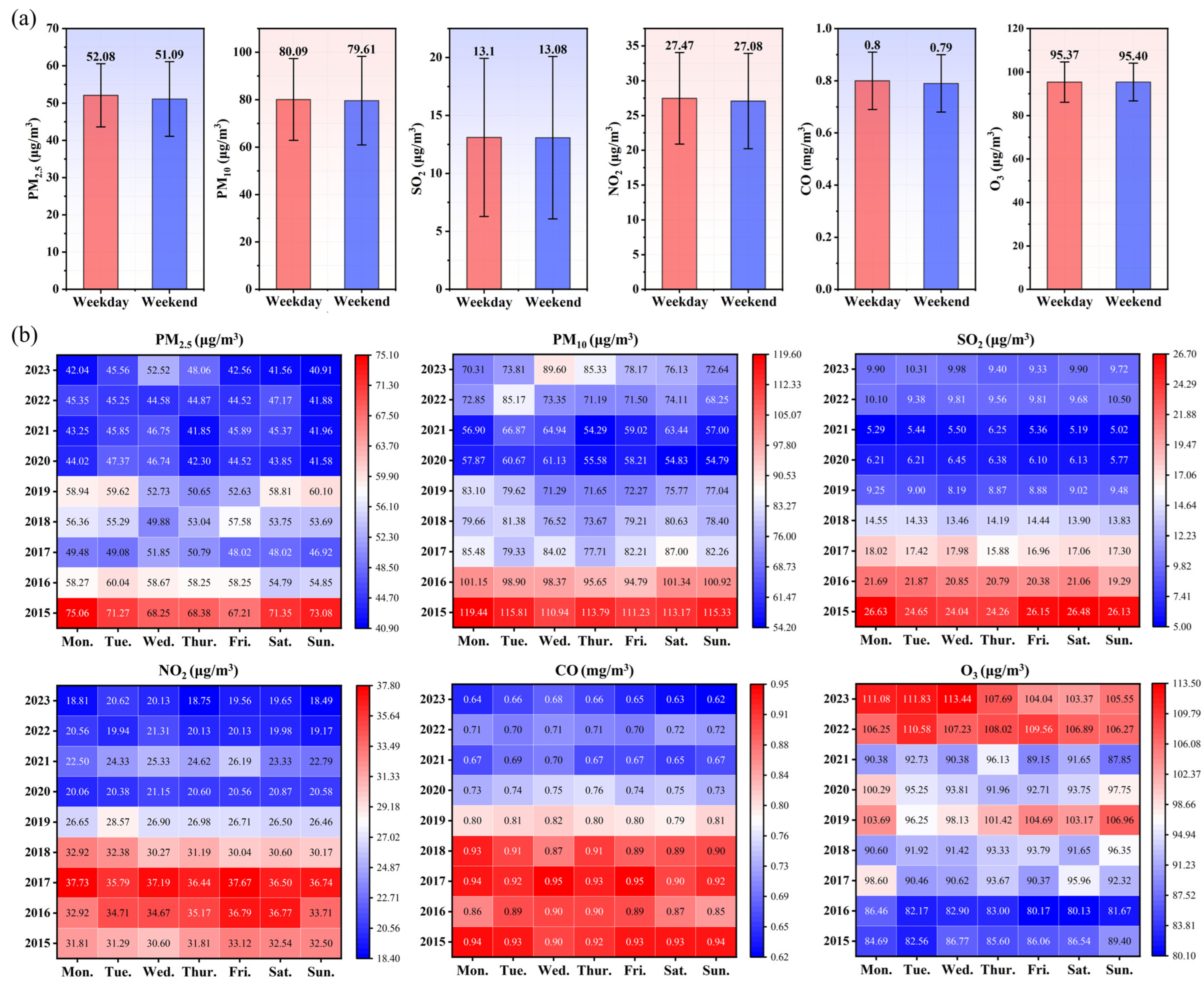
4.1. General Characteristic

A general decline in PM_2.5, PM₁₀, SO₂, NO₂, and CO concentrations was observed in Jingmen city, except for O₃, which exhibited an upward trend (Figure 5). The lowest annual averages of the six air pollutants were concentrated in 2020 and 2021, including PM_2.5 (44.34 μg/m³ in 2020), PM₁₀ (57.59 μg/m³ in 2020), SO₂ (5.44 μg/m³ in 2021), and O₃ (91.18 μg/m³ in 2021) (Figure 5a). This trend was likely due to COVID-19 travel restrictions reducing industrial and transportation activities during 2020–2021. Following the CAAQS standard (Figure 5b), PM_2.5 and PM₁₀ were the predominant pollutants, with 652 and 262 days exceeding the limits, respectively. Moreover, the number of days with O₃ concentration exceeding the standard increased significantly in recent years, gradually becoming one of the primary pollutants in the region. However, CO and SO₂ remained within limits throughout the study period, and NO₂ had no exceedances since 2018, suggesting recent significant improvements in certain air pollutants. Regarding the daily averages (Figure 5c), PM_2.5, PM₁₀, NO₂, and CO displayed a “U-shaped” pattern within the year, which was attributed to seasonal weather conditions [63,64].

However, the intra-annual oscillations in O₃ showed a “mountain-peak” pattern (as opposed to “U-shaped”) (Figure 5c). SO₂ exhibited no consistent pattern of changes, maintaining low levels since 2017. In addition, the fluctuation curve of the daily average PM_2.5 concentration resembled that of PM₁₀, NO₂, and CO, and partially resembled SO₂, suggesting that the five pollutants (PM_2.5, PM₁₀, SO₂, CO, and NO₂) might share similar emission sources, possibly related to coal combustion [49,63]. The general variations in air pollutants in Jingmen city aligned with those observed in other cities of China. Reductions in most air pollutants were primarily attributed to the enforcement of environmental protection laws in China in recent years, with SO₂, NO₂, and CO being better controlled. PM_2.5 and PM₁₀ remained predominant local pollution problems. Furthermore, the escalating trend in O₃ concentration over the years indicated a worsening pollution scenario, mirroring trends in other Chinese cities [65,66].

4.2. Monthly and Seasonal Variations

Figure 6 and Figure 7 illustrate the monthly and seasonal fluctuations in air pollutant concentrations. Except for O₃, concentrations of almost all pollutants peaked in winter (especially in December and January) and valleyed in summer (especially in June and July) (Figure 6 and Figure 7). Moreover, the monthly mean curves of PM_2.5, PM₁₀, SO₂, NO₂, and CO exhibited more pronounced oscillations in winter but gentler transitions in summer (Figure 7b). The difference was especially noticeable for PM_2.5, PM₁₀, and NO₂, with the PM_2.5 concentration (90.65 μg/m³) in winter standing 3.5 times higher than in summer (26.17 μg/m³) (Figure 7a). Seasonal differences also led to a “U-shaped” distribution of monthly averages for PM_2.5, PM₁₀, SO₂, NO₂, and CO.

However, the monthly mean of O₃ showed a bimodal “M-shaped” pattern, peaking in May (118.67 μg/m³) and September (123.09 μg/m³) (Figure 7b). Summer had the highest O₃ concentration (mean: 109.12 μg/m³), but dominance was not significant, while the winter concentration (mean: 66.75 μg/m³) was considerably lower than other seasons (Figure 7a). This finding suggests that the seasonal variations of the O₃ concentration deviated markedly from that of the other five pollutants and did not follow the “winter high, summer low” pattern, with concentrations generally higher from April to October. O₃, categorized as a secondary pollutant, resulted from intricate photochemical reactions involving nitrogen oxides (NO_x) and volatile organic compounds (VOC_S) under sunlight [67,68]. The heightened O₃ levels in warmer seasons likely stemmed from increased solar radiation and escalated photochemical reaction rates, while the diminished concentration in colder seasons might arise from attenuated solar radiation suppressing such reaction rates [65,67].

In general, the seasonal difference in pollutant concentrations in Jingmen was pronounced, with most pollutants following the pattern winter > spring > autumn > summer. Our observations were consistent with previous studies, indicating that the most severe atmospheric pollution occurred during winter [32,69]. The higher pollution concentrations during colder seasons could be attributed to coal and biomass use for heating and stagnant meteorological conditions [70,71]. However, during summer, some significant pollution sources decreased or disappeared, and specific meteorological conditions, such as strong turbulence under intense radiation and high temperatures, along with frequent rainfall, facilitated pollutant removal [72,73]. It was noteworthy that control policies had significantly reduced winter pollutant concentrations recently, leading to a gradual narrowing of seasonal differences. This trend was particularly evident in SO₂ and CO, with more balanced concentration distributions throughout the year since 2017 (Figure 6c,e). Although there was also a decreasing trend of PM₁₀ and NO₂ in winter, further validation over an extended period was necessary (Figure 6b,d). However, the winter pollution situation for PM_2.5 remained concerning, with average concentrations around 100 μg/m³ in January 2022 and 2023, significantly exceeding the CAAQS limit of 75 μg/m³ (Figure 6a).

4.3. Weekdays Versus Weekends

The weekly cycle could be divided into weekdays (from Monday to Friday) and weekends (Saturday and Sunday), representing two typical different lifestyles [31]. Differences in economic activities between weekdays and weekends might affect the weekly cycle in urban air pollutant concentrations [31,73]. In Jingmen city, the weekend and weekday averages for PM_2.5, PM₁₀, SO₂, NO₂, CO, and O₃ remained largely consistent, with differences all less than 2% (Figure 8a). Over nine years, only PM_2.5 and CO concentrations showed higher averages on weekends than on weekdays (5 and 6 times, respectively) (Figure 8b). For PM_2.5 (2015 and 2019), PM₁₀ (2016 and 2019), and O₃ (2015, 2016, and 2019), weekend averages were actually higher than weekdays, reflecting an “anti-weekend effect” (Figure 8b). These results indicate that all air pollutants did not exhibit significant or consistent concentration differences between weekdays and weekends, and the weekly cycling pattern was blurred across all seasons (Figure S1).

However, extensive research showed a notable “weekend effect” in air pollutants, with concentrations typically significantly higher on weekdays than on weekends [73,74]. Studies conducted in Chengdu found that the concentration difference between weekends and weekdays was approximately 5 μg/m³ for PM_2.5 and NO₂ and around 10 μg/m³ for PM₁₀ [31]. These observed “weekend effects” were usually attributed to reduced emissions resulting from decreased human activities on weekends [33,74]. Therefore, the causal relationship naturally led to the “weekend effect” being mainly observed in large, mega, and super-mega cities (i.e., Beijing [74], Chengdu [31], Harbin [75]), where there were collective economic activities with a large population. However, as a small- to medium-sized city, Jingmen has significantly lower population, industrial, and traffic densities compared to the aforementioned cities. Therefore, the influence of human economic activities on the weekly cycling of pollutant concentrations was somewhat weakened, further revealing the close correlation between air pollutant evolution and urban scale.

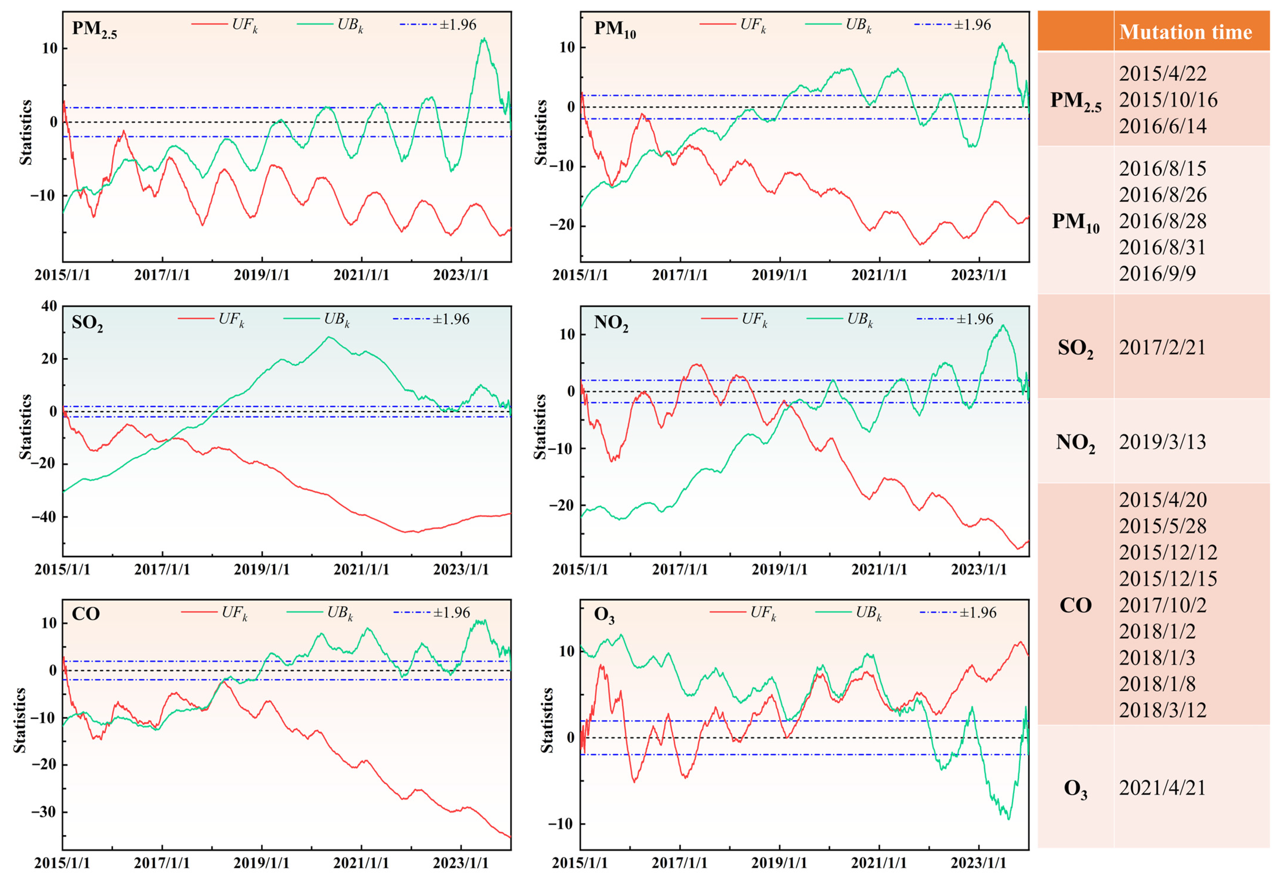
4.4. Mutation Characteristic

Abrupt changes in air pollutant concentrations can swiftly lead to harmful alterations to historic buildings, underscoring the necessity of a stable atmospheric environment [2]. Abrupt changes are characterized by sudden shifts from one statistical feature to another, primarily divided into the following two categories: mean mutations [54] and rate mutations [76]. The Mann–Kendall test effectively analyzed mean mutations, with the intersection of UF_k and UB_k indicating the mutation point [54]. The results (Figure 9) showed multiple occurrences of mean mutations for PM_2.5, PM₁₀, and CO, with the mutation points for PM_2.5 and PM₁₀ clustered before 2017, while CO experienced them in 2015, 2017, and 2018. For SO₂, O₃, and NO₂, intersections occurred only once throughout the study period, on 21 February 2017, 21 April 2021, and 13 March 2019, respectively. Among pollutants, the CO concentration exhibited the most complex pattern of mean mutations, with frequent occurrences and a large span of years. Overall, mutation points were most common in 2015 and 2016 (six times respectively), showing a decreasing trend in frequency over the years. Since 2020, except for O₃, no mutations had occurred, indicating a gradual stabilization of the local air environment. Seasonally, mean mutations were more prevalent in spring and winter, highlighting the significant role of meteorological factors. Previous research also suggested that stagnant meteorological conditions often led to severe pollution events, common in low-temperature seasons [77,78].

Additionally, the MK test for trend analysis and linear trends (Figure 5c) of air pollutant sequences was consistent. Starting in late January 2015, UF_k values for PM_2.5, PM₁₀, SO₂, and CO were all <0, exceeding the confidence interval, indicating a significant decrease. NO₂ also displayed a persistent decline since 2018. However, O₃ showed an overall upward trend, particularly after May 2019, with UF_k values surpassing the confidence interval, indicating a significant increase.

A common method for identifying rate mutations involves reconstructing the first-level high-frequency coefficients using discrete wavelet decomposition, with mutations occurring at times corresponding to points with large coefficients [37,76]. The results (Figure 10) showed that, from 2015 to 2023, PM_2.5, SO₂, NO₂, and CO exhibited a declining trend in mutation frequency. However, there was a slight increase in both the frequency and magnitude for PM₁₀ and O₃ over time. Among pollutants, SO₂ mutations were the most stable, characterized by low frequency and small magnitude, with most occurring before 2017. Similarly, after 2017, there was a significant decrease in CO mutations. Overall, the rate mutations of all air pollutants were more prevalent during cold seasons, with PM_2.5, NO₂, and CO exhibiting higher rates during winter, while PM₁₀ mutations were mainly observed in spring. Further, rate mutations in O₃ displayed a more complex and frequent pattern, without a consistent seasonal trend. This finding suggests that O₃ evolution responded more intricately to changes in emissions due to the nonlinear effects of meteorological conditions and precursor emissions [32,79].

Moreover, after five-layer wavelet decomposition filtering, the high-frequency signal pattern for the PM_2.5 concentration closely resembled PM₁₀, indicating that they shared a similar source [32,63]. However, rate mutations for PM₁₀ consistently lagged behind PM_2.5 by approximately two months, primarily occurring in spring rather than winter, likely due to sand-dust weather. With rising temperatures in spring, the thawing of frozen soil and the loosening of surface soil, coupled with frequent strong winds, contribute to occurrences of sand-dust weather [69]. Dust particles typically had diameters greater than 2.5 μm, leading to rapid increases in PM₁₀ concentration [80].Therefore, pollution mitigation efforts should not only address the coordinated control of PM_2.5 and PM₁₀ but also implement targeted interventions based on particle size differences under specific meteorological conditions.

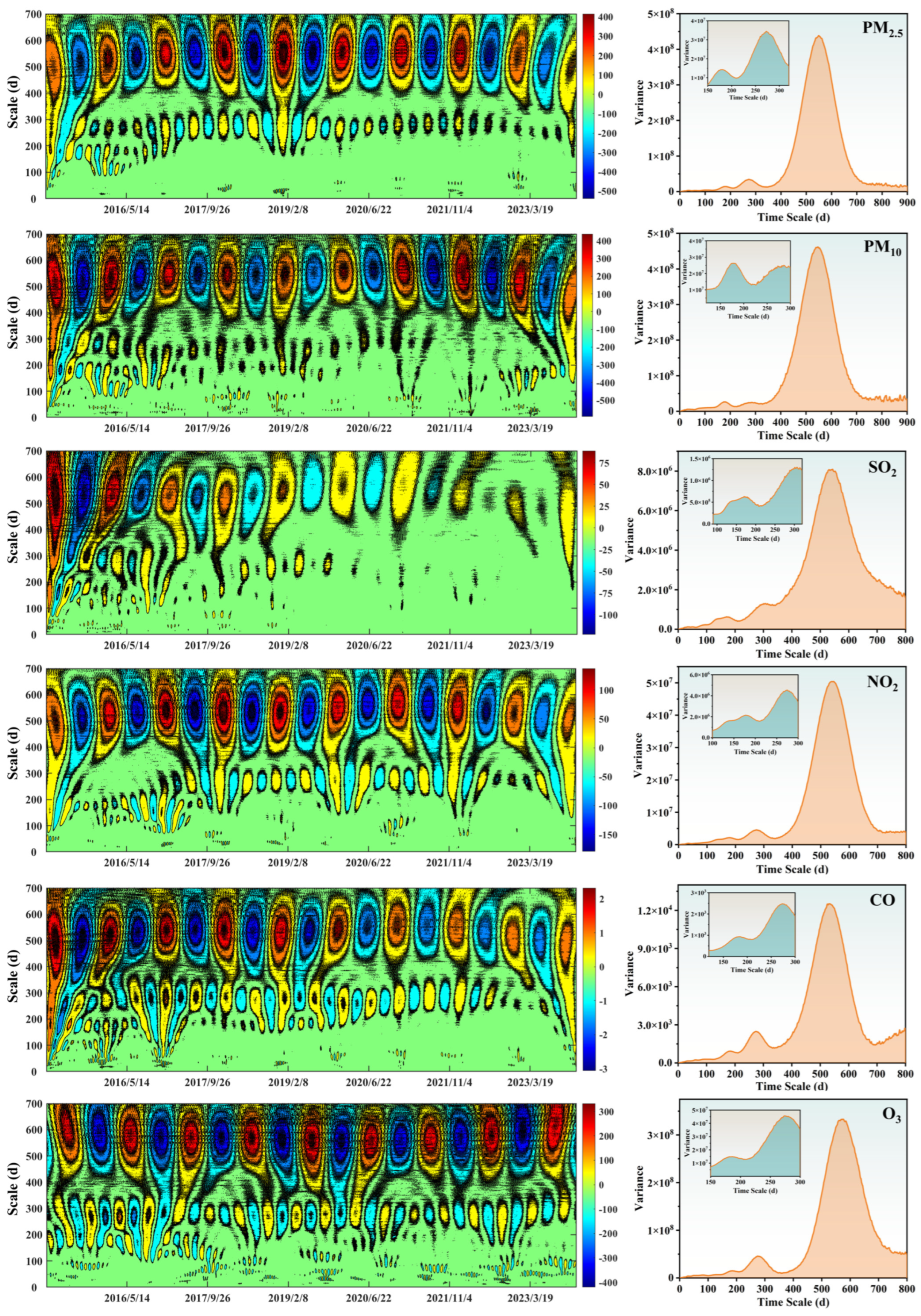
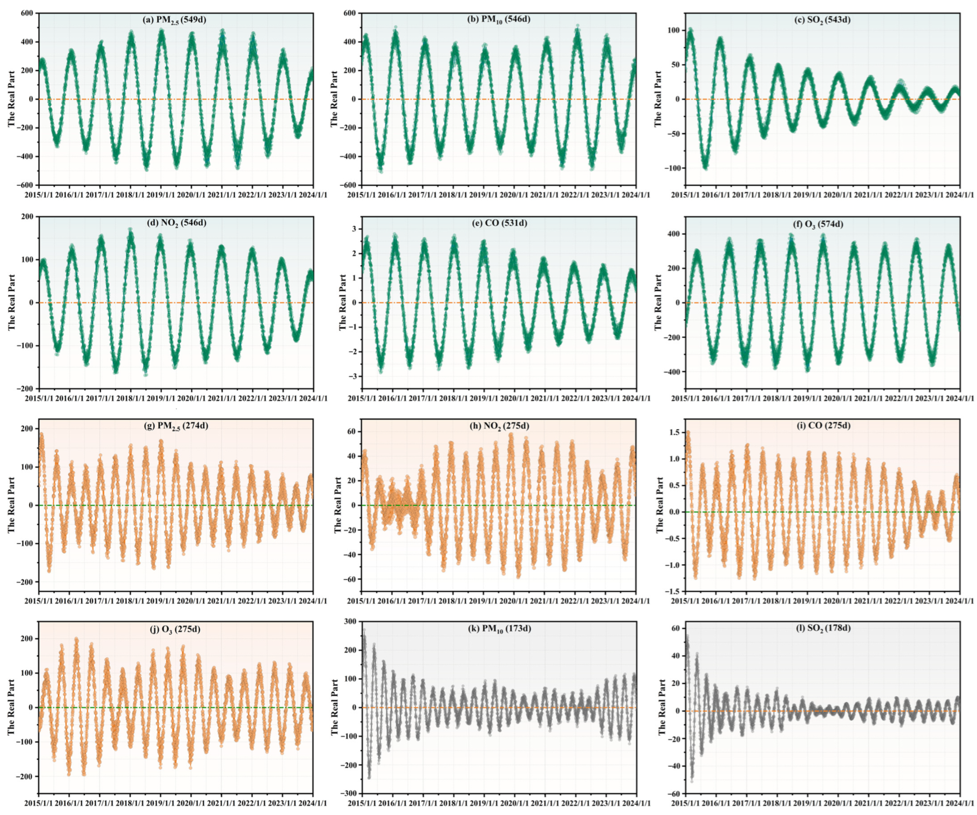
4.5. Periodic Characteristic

The temporal evolution of air pollutant concentrations exhibited non-stationary behavior with varying dominant cycles on different scales, and wavelet analysis adeptly described these cyclical patterns [45]. The real part of wavelet coefficients (Figure 11, left) indicated the energy distributions of air pollutants over time, frequency, and scale, with their periods largely overlapping, particularly on the scales of 150–200 d, 250–300 d, and 450–600 d. Among these, there were obvious oscillations on the 450–600 d scale, and the periodic characteristics were very stable in the entire evolutionary process. While SO₂ exhibited weakened oscillations after 2021, the stability of this scale remained consistent for other pollutants. Moreover, PM_2.5, PM₁₀, NO₂, and CO displayed similar fluctuation patterns on the 450–600 d scale, with ten high-value centers and nine low-value centers across the time domain, primarily occurring around 8–18 January and 7–13 July each year, respectively. High concentrations were observed during the first and last three months of the year (January to March and October to December), while lower concentrations were evident during the intervening six months (April to September). The energy distributions aligned well with the seasonal variations in air pollutants, further suggesting that these four pollutants (PM_2.5, PM₁₀, NO₂, and CO) might originate from similar emission sources [63].

However, while O₃ also exhibited a significant oscillation period on the 400–700 d scale, only nine high-value centers and eight low-value centers were present. The time distributions of high and low concentrations differed from other pollutants, with high values mainly occurring from March to September, spanning 8 months. Significant periodic oscillations were also observed for PM_2.5, NO₂, CO, and O₃ on the 250–300 d scale, largely covering the entire domain. However, the smaller scale oscillation for 150–200 d was more prominent before 2017, primarily observed in PM₁₀ and SO₂. For instance, PM₁₀ experienced four conversions between January 2015 and March 2016, with a cycle of two months and peak intervals of about one month.

The variance of wavelet coefficient (Figure 11, right) further examined the amplitude modulation, and the variance values showed the power of the fluctuations, with higher values being the more dominant oscillations on that scale [45]. The results revealed that the highest peaks of wavelet variance for six air pollutants fell within the range of 531–574 d (PM_2.5-549 d, PM₁₀-546 d, SO₂-543 d, NO₂-546 d, CO-531 d, O₃-574 d), indicating the strongest periodic oscillations on this scale. Moreover, PM_2.5, NO₂, CO, and O₃ exhibited a similar second dominant cycle (274–275 d); however, the peak was weaker and less energetic than the first dominant period. Overall, fluctuations on these two scales almost entirely controlled the variations of the daily average concentrations across the entire time domain. In addition, although PM₁₀ and SO₂ showed no cycle on the scale of 274–275 d, they both shared a weaker peak on the 170–180 d scale.

Based on wavelet variance analysis, the real part variations of the three dominant periods (531–574 d, 274–275 d, and 170–180 d) were illustrated (Figure 12). On the scale of 531–574 d, two up-down conversions happened in an annual cycle (Figure 12a–f). High values were observed mainly from November to April, while low values occurred predominantly from May to October. For the first primary period, both SO₂ and CO showed a weakening trend in fluctuation amplitudes over time. However, PM_2.5 and NO₂ exhibited a “strong in the middle, weak at both ends” pattern (Figure 12a,d), while PM₁₀ showed the opposite (“weak in the middle, strong at both ends”) (Figure 12b). Typically, most NO₂ emissions came from fossil fuel combustion, biomass burning, soil, and various industrial sources [81]; hence, the observed similarity between parts of the NO₂ curve and the PM_2.5 curve was not surprising.

For the second dominant period (274–275 d), PM_2.5, NO₂, CO, and O₃ all experienced two up-down conversions within about 180 days (Figure 12g–j). High values were mainly observed from mid-November to January and from May to July. However, on the scale of 170–180 d, the up-down conversion for PM₁₀ and SO₂ was approximately within 120 days (Figure 12k,l). On both the 274–275 d and 170–180 d scales, PM_2.5, PM₁₀, SO₂, and CO demonstrated a declining trend in amplitude over the study period. In addition, O₃ exhibited different distributions of high and low values across the time domain despite sharing similar periodicities with other pollutants (Figure 12f,j). High O₃ concentration was mainly observed from April to September on the 531–574 d scale, while on the 274–275 d scale, high values occurred from March to May and from July to September. This finding was consistent with the multi-year monthly average variation curve of O₃ (Figure 7b, last image).

The analysis above revealed the dominant periods, conversions between high and low values, and time distributions of pollutant concentration sequences, highlighting the heterogeneous, multilayer structure and pronounced localization of the sequences across entire time domain. The annual period was commonly observed in the evolution of all air pollutants, consistent with numerous research findings [37,45]. However, the scales of 274–275 d and 170–180 d were relatively uncommon in other cities, confirming the regional differences in medium- and small-scale cycles [37]. The periodic scales of 274–275 d and 170–180 d align closely with seasonal changes, suggesting a potential connection to the monsoon climate, fluctuations in industrial production, and the seasonal demand for heating. Therefore, localized control strategies for air pollutants should pay particular attention to periodicities on medium and small scales. Furthermore, due to successive environmental governance policies implemented, significant differences in periodic amplitude changes for different pollutants have emerged. These differences emphasized trend analysis in precise periodic control of various pollutants, which might have been overlooked in previous studies.

5. Correlations Between Air Pollutants

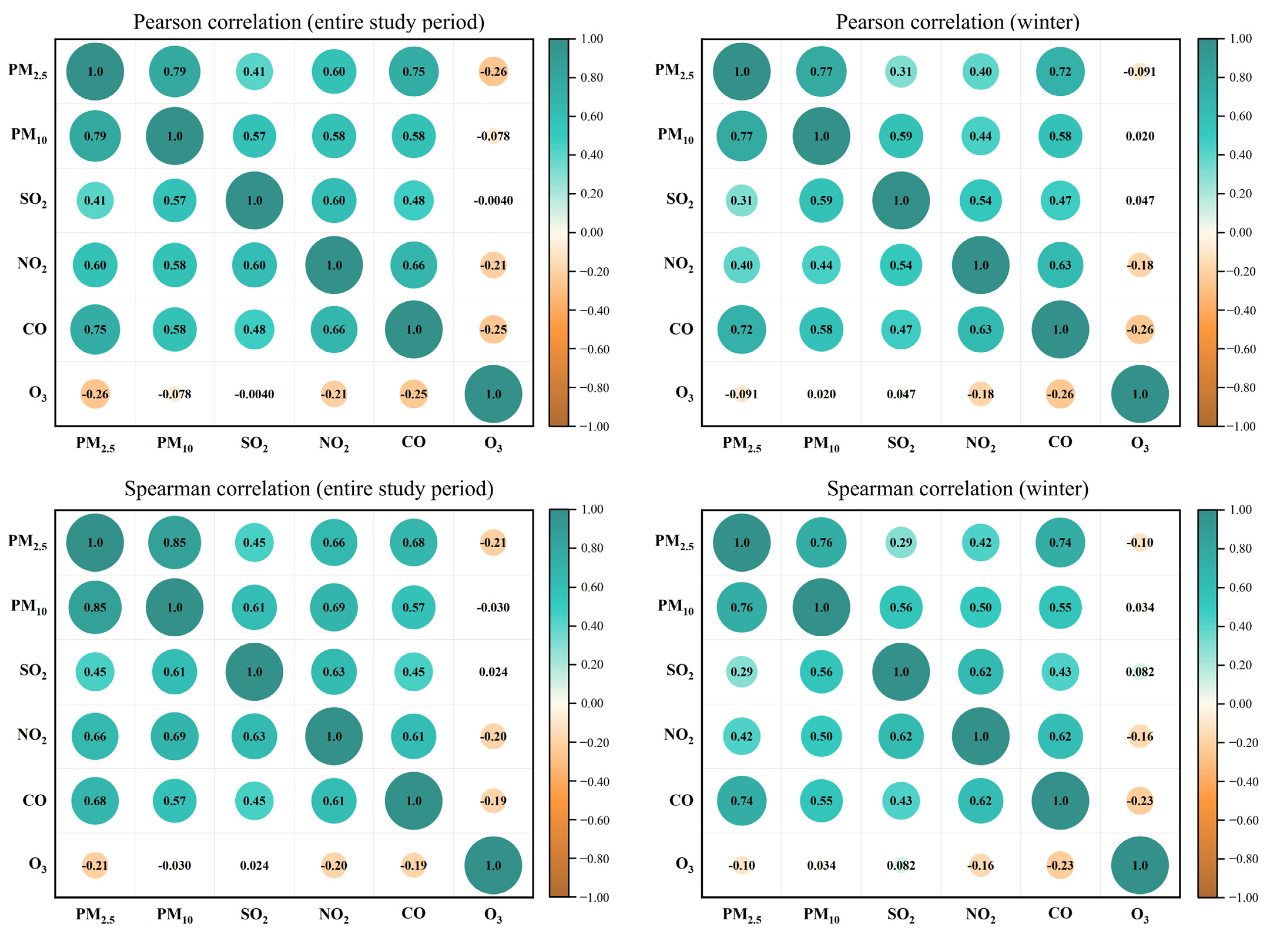
5.1. Pearson and Spearman Correlation

Pearson and Spearman correlations were conducted to assess the overall correlations among the six air pollutants over the entire study period, and the findings from both methods exhibited strong consistency (Figure 13). All pairs of pollutants, including PM_2.5, PM₁₀, SO₂, NO₂, and CO, demonstrated positive correlations. The correlation between PM₁₀ and PM_2.5 was the strongest (r = 0.79, ρ = 0.85), indicating significant synergies between the emissions of particles of varying sizes [38]. Further, PM_2.5-CO (r = 0.75, ρ = 0.68) and PM_2.5-NO₂ (r = 0.60, ρ = 0.66) showed good positive correlations, attributable to the fact that both CO and NO₂ emissions tended to be accompanied by PM_2.5, which had similar sources like fossil fuel combustion and automobile exhaust [36,37]. However, owing to precursor-to-O₃ conversion trends, multiple air pollutants displayed relatively weak negative correlations with O₃ [32]. Among these, a negative correlation between PM_2.5 and O₃ was observed (r = −0.26, ρ = −0.21), suggesting that higher PM_2.5 concentrations might have an impact on the secondary formation of O₃ [82]. In addition, correlations between any pairs of air pollutants during winter weakened compared to the entire study period.

5.2. Wavelet Coherence Analysis

Further investigation was to determine whether the overall correlations indicated by the Pearson and Spearman results exhibited consistency across all time scales. The WTC (Figure 14 and Figure S2) revealed the full-time multi-scale correlations between air pollutants, including resonance periods, coherent distributions, and time-lag characteristics. The average power of the wavelet coherence (AWC) and the percent area of significant coherence (PASC) values from the WTCs are shown in

Table 1. Average power of the wavelet coherence (AWC) and percent area of the significant coherence (PASC) of wavelet coherence (WTC).

Variables	Entire Study Period		Winter
	AWC	PASC (%)	AWC	PASC (%)
PM2.5-PM10	0.7170	59.90%	0.6933	54.52%
PM2.5-SO2	0.4068	15.55%	0.3522	8.37%
PM2.5-NO2	0.5165	29.48%	0.4792	19.08%
PM2.5-CO	0.5950	43.78%	0.6667	50.42%
PM2.5-O3	0.5062	26.15%	0.4042	9.26%
PM10-SO2	0.4978	25.56%	0.4740	17.63%
PM10-NO2	0.5292	31.29%	0.4624	19.43%
PM10-CO	0.5361	27.88%	0.5159	28.23%
PM10-O3	0.4491	23.58%	0.3676	8.64%
SO2-NO2	0.5176	29.91%	0.4467	20.92%
SO2-CO	0.4341	17.69%	0.3451	6.45%
SO2-O3	0.4326	20.41%	0.3907	12.32%
NO2-CO	0.5371	29.46%	0.5132	26.63%
NO2-O3	0.4858	23.15%	0.4171	15.56%
CO-O3	0.4206	20.61%	0.3416	9.49%

. The results illustrated a significant positive correlation between PM_2.5 and PM₁₀ across all time scales. When comparing the AWC and PASC, PM_2.5-PM₁₀ had the highest values (AWC = 0.7170, PASC = 59.90%). PM_2.5 and PM₁₀ demonstrated numerous in-phase coherent distributions (Figure 14a), indicating synchronized variations and highlighting their significant inclusive relationship. Moreover, PM_2.5 exhibited relatively continuous high-energy resonances with NO₂, CO, and O₃ on the scale of 128–512 d (Figure 14c–e). Among these, PM_2.5 showed positive correlations with CO and NO₂, while it displayed a negative correlation with O₃. Furthermore, PM₁₀ and the four pollutants (SO₂, NO₂, CO, and O₃) exhibited similar patterns of coherent distributions, primarily concentrated at large time scales (256–512 d), showing continuous periodic resonances throughout the entire domain (Figure 14f–i). However, differences existed in the phase relationships within these coherent regions. Except for O₃, PM₁₀ was mainly positively correlated with the other three pollutants.

Notably, the correlations between O₃ and PM_2.5 or PM₁₀ exhibited significant time-scale dependency (Figure 14e,i). At larger scales (e.g., annual scale), their negative correlation remained consistent throughout the study period. However, at smaller scales (e.g., monthly scale), a certain positive effect between O₃ and PM_2.5 or PM₁₀ responses was observed, primarily occurring in summer. This phenomenon of phase relationship changing with resonance scale also occurred in the coherent distributions of SO₂-O₃ and NO₂-O₃ (Figure 14l,n). The negative correlation between O₃ and multiple pollutants on larger scales was speculated to be due to the decrease in concentrations of other pollutants, which reduced the scattering and absorption of sunlight and increased UV radiation, favoring O₃ formation [37,68]. However, in summer, high temperatures and intense solar radiation promoted both the formation of photochemical product O₃ and secondary particles significantly [83]. Therefore, synchronous increases and decreases between multiple pollutants (i.e., PM_2.5, PM₁₀) and O₃ were observed at smaller scales during the summer.

Furthermore, NO₂ and CO had a strong correlation on medium to large scales (128–512 d), but on smaller scales (<128 d), their coherence was markedly weakened, with only a few regions passing the significance test (Figure 14m). Specifically, there were significant in-phase positive coherent distributions between NO₂ and CO on the scale of 256–512 d, suggesting that CO could directly lead to the increase of NO₂ within this oscillation period. However, on smaller scales, the relationship between SO₂ and NO₂ was more tightly connected, with a large number of intermittent positive coherent distributions on the scale of 16–64 d (Figure 14j). The strong correlation of SO₂-NO₂ (AWC = 0.5176, PASC = 29.91%) might be attributed to their involvement in the production of secondary aerosols (including sulfates, nitrates, etc.) [84].

Moreover, the coherence between PM_2.5 and SO₂ was the weakest among all combinations, with the lowest being AWC (0.4068) and PASC (15.55%). This finding differed significantly from prior research, which suggested a high degree of similarity in the WTC results for PM_2.5-SO₂ and PM_2.5-NO₂ [38]. However, in our investigation, the correlation of PM_2.5-SO₂ was significantly weaker than that of PM_2.5-NO₂, possibly due to the substantial decline in SO₂ concentration in recent years. It was noteworthy that there was a lag in PM_2.5 changes in several coherent distributions for both PM_2.5-SO₂ and PM_2.5-NO₂ (Figure 14b,c). The delayed impact of NO₂ and SO₂ on PM_2.5 arose from their involvement in the secondary generation of PM_2.5, and the conversion process occurred under specific conditions [37]. This further elucidated why the correlation between PM_2.5-SO₂ and PM_2.5-NO₂ increased with the expansion of the time scale.

In addition, seasonal characteristics of the correlations between six air pollutants were analyzed. On the scale of 256–512 d (approximately annual), all combinations showed continuous coherent patterns with minimal seasonal influence. On larger scales (>512 d), coherent distributions were observed only between CO and SO₂. However, on smaller scales (<256 d), seasonal differences in the correlations among air pollutants became apparent. For example, intermittent coherent distributions of SO₂-NO₂ on the 30 d scale were concentrated in the spring, autumn, and winter, with weaker coherence observed in summer (Figure 14j). Conversely, coherence between SO₂ and O₃ on the same scale was concentrated in spring and autumn (Figure 14l). In general, resonances of air pollutants on small time scales were less frequent during the summer. The comparison of PASC values in the entire study period and in winter (Figure 14 and Figure 15, Table 1) showed that only the winter PASC values for PM_2.5-CO and PM₁₀-CO were higher, primarily increasing at smaller scales (4–64 d), particularly evident in the enlargement of coherent regions on the 16–32 d scale. However, this strengthening of resonances was intermittent, with increases mainly occurring in December. In January and February in winter, these coherent distributions experienced multiple interruptions. Therefore, particular attention should be paid to the synergistic control of PM_2.5 or PM₁₀ and CO in December.

The analysis presented above revealed coupling resonances of six air pollutants in Jingmen city across multiple time-frequency scales. Fifteen pairs of variables formed three distinctive resonance periods: annual, quadrennial, and monthly. Across most large-scale resonances, the phase angles remained stable, with continuous coherent distributions. However, on small and medium scales, correlations became complex, marked by fluctuating phase angles and intermittent coherent distributions, showing seasonal differences. Among pollutants, the most stable resonance occurred between PM_2.5 and PM₁₀, while the most complex one emerged between O₃ and other pollutants.

6. Discussion

6.1. Discussion of the Link Between Material Properties and Air Pollutants

The study presents a comprehensive analysis of both the material characteristics of the black stains on the stone substrate and the temporal evolution of air pollutants in Jingmen city. The petrographic analysis of the marble fragments (both dolomitic and calcitic) reveals that the stone’s composition, including the presence of calcite, dolomite, and other trace minerals, plays a crucial role in understanding the potential for pollutant deposition and surface alteration. The SEM-EDS results show that the black stains on the marble are largely composed of carbonaceous particles, metals, and silicon, indicating that air pollution, particularly PM, CO, SO₂, and NO₂, has significantly contributed to the degradation of the stone surface. In parallel, the air quality data from Jingmen, showing seasonal and inter-annual variations in the concentrations of pollutants like PM_2.5, PM₁₀, SO₂, NO₂, CO, and O₃ provide a clear picture of the pollution trends and their potential impact on the preservation of cultural heritage. The strong correlations between pollutants, especially PM_2.5 and PM₁₀, indicate a synergistic effect of particulate pollution on both the environment and stone structures.

One of the major challenges in this work is connecting the two distinct areas of analysis, material characterization and air pollution data. However, the correlation between the accumulation of carbonaceous and metallic particles on the surface of the stone and the concentration of air pollutants is evident. As pollutants, especially PM, SO₂, NO₂, and O₃, increase in concentration, they contribute to the deposition of these pollutants on the surface of the marble, leading to the formation of black stains and surface degradation. This temporal correlation between the rise in pollution levels and the deterioration of the stone substrate highlights the need for a deeper understanding of the interactions between atmospheric pollutants and the material properties of cultural heritage objects. Moreover, the seasonal cycles of pollutant concentrations, particularly the higher concentrations in winter, align with the period of increased degradation of the stone surfaces, further emphasizing the connection between pollutant exposure and material deterioration.

There is a need for further investigation into the long-term effects of combined pollutants (PM, SO₂, NO₂, CO, and O₃) on stone substrates to better predict and prevent future damage. The interaction between various pollutants, such as their synergistic effects on enhancing surface degradation or their role in catalyzing the sulfation and carbonization processes, should be explored in more detail. Additionally, future research should focus on developing models that simulate the impact of air quality variations on the degradation of stone materials over extended periods, integrating both the chemical and physical factors. This would provide a more robust framework for heritage conservation. It would also be beneficial to study the role of meteorological factors, such as humidity and temperature, in these degradation processes, as these factors could influence the deposition and chemical reactions on the stone surfaces.

6.2. Discussion of the Protection Strategies and Measures

Given the significant role of air pollutants, particularly particulate matter (PM_2.5, PM₁₀), SO₂, NO₂, and O₃, in the degradation of the stone, a multi-pronged approach is necessary to mitigate these pollutants. Strategies include:

o

Emission Controls: Implementing stricter regulations on industrial emissions, particularly for sources that contribute to SO₂, NO₂, and particulate matter is one strategy. The enforcement of low-emission technologies and cleaner fuels in transportation and industry could significantly reduce the concentrations of these pollutants.

o

Urban Green Spaces: Expanding green spaces and vegetation cover in the vicinity of historical sites can help absorb pollutants and reduce the overall pollution load in the air. Additionally, trees and plants can act as passive filters, trapping particulate matter and reducing the direct impact on stone surfaces.

o

Air Quality Monitoring: The continuous monitoring of air pollutants in and around cultural heritage sites will allow for real-time assessment and targeted interventions. Real-time data on pollutant concentrations will help heritage professionals adjust conservation strategies in response to spikes in pollution levels.

In addition to controlling pollutant emissions, protective measures for the stone surfaces are essential. Strategies include:

o

Protective Coatings: One strategy involves the application of protective coatings that can shield the stone from direct contact with pollutants and reduce the deposition of particulate matter. These coatings should be breathable, allowing moisture to escape while preventing the penetration of pollutants.

o

Regular Cleaning and Maintenance: A strategy for this involves implementing a routine cleaning and conservation program to remove accumulated pollutants from stone surfaces before they cause significant damage. The use of mild cleaning agents and techniques that do not harm the integrity of the stone is critical. Some laser micro- and nano-processing technologies [85,86,87,88], such as the preparation of hydrophobic structures [89], laser cleaning [90], can have significant advantages in their non-contact, non-contaminating approach.

o

Surface Treatments for Acid Rain Protection: Given the impact of SO₂ and NO₂ on stone surfaces through acid rain formation, the use of surface treatments that neutralize the effects of acidic compounds should be explored. This can include the use of alkaline treatments that help prevent the sulfation process, which leads to further degradation.

By addressing both the environmental factors and the protection of the stone substrates, these strategies will help preserve cultural heritage in the face of ongoing urban pollution. Combining pollutant control with surface protection will provide a holistic approach to mitigating the impact of air pollution on historical stone structures, ensuring their longevity for future generations.

7. Conclusions

In the Xianling Tomb, located in Jingmen city, a designated World Heritage Site, widespread black stains observed on marble buildings were confirmed to result from prolonged exposure to various air pollutants. Effectively controlling and predicting pollutant concentrations contributed to addressing preservation challenges, requiring a scientific understanding of their temporal evolution patterns. The main conclusions are as follows.

(1) This study confirmed that the Xianling Tomb’s construction stones are dolomitic and calcitic marbles, both of which are vulnerable to environmental degradation. The black stains altered the stone’s microstructure, increasing porosity and weakening cohesion. SEM-EDS analysis revealed the significant enrichment of carbonaceous particles, metallic elements, and sulfur, indicating prolonged exposure to air pollutants like PM and SO₂.

(2) In the context of air pollutants, our study shows that recent improvements in SO₂, CO, and NO₂ were relatively significant, with PM_2.5, PM₁₀, and O₃ constituting the most severe problems. Combining phase differences between PM and O₃ in resonances at different time scales provided a viable approach for their coordinated control.

(3) Results indicated significant non-stationarity, multiscale, and localized characteristics of pollutant concentrations. Seasonal differences were observed, while monthly averages exhibited a “U”-shaped pattern and no discernible “weekend effect”. Mutations frequently occurred during colder seasons, correlating with adverse meteorological conditions, with rate mutations being more severe, frequent, and temporally complex.

(4) The analysis identified three key resonance periods (annual, quadrennial, and monthly) among six air pollutants in Jingmen City. PM_2.5 and PM₁₀ showed the strongest correlation, while O₃ had the most complex relationships, varying by time scale and season. Winter correlations weakened overall, except for stronger PM_2.5-CO and PM₁₀-CO coherence in December, highlighting the need for targeted pollution control.

Future efforts will focus on applying protective coatings or sealants to stone surfaces to reduce the penetration of pollutants such as O₃ and PM_2.5, thereby mitigating their effects. Additionally, ongoing environmental monitoring and air quality management will be crucial in regions with high pollution levels, helping to control pollutant concentrations and protect historical monuments from further deterioration.

References

1. Mitsos, D.; Kantarelou, V.; Palamara, E.; Karydas, A.; Zacharias, N.; Gerasopoulos, E. Characterization of black crust on archaeological marble from the Library of Hadrian in Athens and inferences about contributing pollution sources. J. Cult. Heritage 2022, 53, 236–243. [Google Scholar] [CrossRef]
2. Basu, S.; Orr, S.A.; Aktas, Y.D. A Geological Perspective on Climate Change and Building Stone Deterioration in London: Implications for Urban Stone-Built Heritage Research and Management. Atmosphere 2020, 11, 788. [Google Scholar] [CrossRef]
3. Rosso, F.; Jin, W.; Pisello, A.L.; Ferrero, M.; Ghandehari, M. Translucent marbles for building envelope applications: Weathering effects on surface lightness and finishing when exposed to simulated acid rain. Constr. Build. Mater. 2016, 108, 146–153. [Google Scholar] [CrossRef]
4. Moropoulou, A.; Tsiourva, T.; Bisbikou, K.; Tsantila, V.; Biscontin, G.; Longega, G.; Groggia, M.; Dalaklis, E.; Petritaki, A. Evaluation of cleaning procedures on the facades of the Bank of Greece historical building in the center of Athens. Build. Environ. 2002, 37, 753–760. [Google Scholar] [CrossRef]
5. Samara, C.; Melfos, V.; Kouras, A.; Karali, E.; Zacharopoulou, G.; Kyranoudi, M.; Papadopoulou, L.; Pavlidou, E. Morphological and geochemical characterization of the particulate deposits and the black crust from the Triumphal Arch of Galerius in Thessaloniki, Greece: Implications for deterioration assessment. Sci. Total Environ. 2020, 734, 139455. [Google Scholar] [CrossRef]
6. Böke, H.; Göktürk, E.H.; Saltık, E.N.C. Effect of some surfactants on SO2–marble reaction. Mater. Lett. 2002, 57, 935–939. [Google Scholar] [CrossRef]
7. La Russa, M.F.; Fermo, P.; Comite, V.; Belfiore, C.M.; Barca, D.; Cerioni, A.; De Santis, M.; Barbagallo, L.F.; Ricca, M.; Ruffolo, S.A. The Oceanus statue of the Fontana di Trevi (Rome): The analysis of black crust as a tool to investigate the urban air pollution and its impact on the stone degradation. Sci. Total Environ. 2017, 593-594, 297–309. [Google Scholar] [CrossRef]
8. Saba, M.; Quiñones-Bolaños, E.; López, A.L.B. A review of the mathematical models used for simulation of calcareous stone deterioration in historical buildings. Atmos. Environ. 2018, 180, 156–166. [Google Scholar] [CrossRef]
9. Russa, M.F.; Belfiore, C.M.; Comite, V.; Barca, D.; Bonazza, A.; Ruffolo, S.A.; Crisci, G.M.; Pezzino, A. Geochemical study of black crusts as a diagnostic tool in cultural heritage. Appl. Phys. A 2013, 113, 1151–1162. [Google Scholar] [CrossRef]
10. Lal, R.M.; Nagpure, A.S.; Luo, L.; Tripathi, S.N.; Ramaswami, A.; Bergin, M.H.; Russell, A.G. Municipal solid waste and dung cake burning: Discoloring the Taj Mahal and human health impacts in Agra. Environ. Res. Lett. 2016, 11, 104009. [Google Scholar] [CrossRef]
11. Ogrizek, M.; Gregorič, A.; Ivančič, M.; Contini, D.; Skube, U.; Vidović, K.; Bele, M.; Šala, M.; Gunde, M.K.; Rigler, M.; et al. Characterization of fresh PM deposits on calcareous stone surfaces: Seasonality, source apportionment and soiling potential. Sci. Total Environ. 2022, 856, 159012. [Google Scholar] [CrossRef] [PubMed]
12. Giavarini, C.; Santarelli, M.; Natalini, R.; Freddi, F. A non-linear model of sulphation of porous stones: Numerical simulations and preliminary laboratory assessments. J. Cult. Heritage 2008, 9, 14–22. [Google Scholar] [CrossRef]
13. Agelakopoulou, T.; Metaxa, E.; Karagianni, C.-S.; Roubani-Kalantzopoulou, F. Air pollution effect of SO2 and/or aliphatic hydrocarbons on marble statues in Archaeological Museums. J. Hazard. Mater. 2009, 169, 182–189. [Google Scholar] [CrossRef] [PubMed]
14. Çetintaş, S.; Akboğa, Z. Investigation of resistance to ageing by SO2 on some building stone. Constr. Build. Mater. 2020, 262, 120341. [Google Scholar] [CrossRef]
15. Luque, A.; de Yuso, M.V.M.; Cultrone, G.; Sebastián, E. Analysis of the surface of different marbles by X-ray photoelectron spectroscopy (XPS) to evaluate decay by SO2 attack. Environ. Earth Sci. 2012, 68, 833–845. [Google Scholar] [CrossRef]
16. Lan, T.T.N.; Nishimura, R.; Tsujino, Y.; Satoh, Y.; Thoa, N.T.P.; Yokoi, M.; Maeda, Y. The effects of air pollution and climatic factors on atmospheric corrosion of marble under field exposure. Corros. Sci. 2005, 47, 1023–1038. [Google Scholar] [CrossRef]
17. Barca, D.; Comite, V.; Belfiore, C.M.; Bonazza, A.; La Russa, M.F.; Ruffolo, S.A.; Crisci, G.M.; Pezzino, A.; Sabbioni, C. Impact of air pollution in deterioration of carbonate building materials in Italian urban environments. Appl. Geochem. 2014, 48, 122–131. [Google Scholar] [CrossRef]
18. Di Turo, F.; Proietti, C.; Screpanti, A.; Fornasier, M.F.; Cionni, I.; Favero, G.; De Marco, A. Impacts of air pollution on cultural heritage corrosion at European level: What has been achieved and what are the future scenarios. Environ. Pollut. 2016, 218, 586–594. [Google Scholar] [CrossRef]
19. Dan, M.B.; Přikryl, R.; Török, Á. Materials, Technologies and Practice in Historic Heritage Structures; Springer: Berlin/Heidelberg, Germany, 2010. [Google Scholar]
20. Vidorni, G.; Sardella, A.; De Nuntiis, P.; Volpi, F.; Dinoi, A.; Contini, D.; Comite, V.; Vaccaro, C.; Fermo, P.; Bonazza, A. Air pollution impact on carbonate building stones in Italian urban sites⋆. Eur. Phys. J. Plus 2019, 134, 439. [Google Scholar] [CrossRef]
21. Fermo, P.; Turrion, R.G.; Rosa, M.; Omegna, A. A new approach to assess the chemical composition of powder deposits damaging the stone surfaces of historical monuments. Environ. Sci. Pollut. Res. 2014, 22, 6262–6270. [Google Scholar] [CrossRef]
22. Comite, V.; Álvarez de Buergo, M.; Barca, D.; Belfiore, C.M.; Bonazza, A.; La Russa, M.F.; Pezzino, A.; Randazzo, L.; Ruffolo, S.A. Damage monitoring on carbonate stones: Field exposure tests contributing to pollution impact evaluation in two Italian sites. Constr. Build. Mater. 2017, 152, 907–922. [Google Scholar] [CrossRef]
23. Bergin, M.H.; Tripathi, S.N.; Devi, J.J.; Gupta, T.; Mckenzie, M.; Rana, K.S.; Shafer, M.M.; Villalobos, A.M.; Schauer, J.J. The Discoloration of the Taj Mahal due to Particulate Carbon and Dust Deposition. Environ. Sci. Technol. 2014, 49, 808–812. [Google Scholar] [CrossRef] [PubMed]
24. Kirkitsos, P.; Sikiotis, D. Deterioration of Pentelic marble, Portland limestone and Baumberger sandstone in laboratory exposures to NO2: A comparison with exposures to gaseous HNO3. Atmos. Environ. 1996, 30, 941–950. [Google Scholar] [CrossRef]
25. Massey, S. The effects of ozone and NOx on the deterioration of calcareous stone. Sci. Total. Environ. 1999, 227, 109–121. [Google Scholar] [CrossRef]
26. Haneef, S.; Johnson, J.; Thompson, G.; Wood, G. Effects of dry deposition of pollutant gases on the degradation of pentelic marble. Corros. Sci. 1993, 35, 743–750. [Google Scholar] [CrossRef]
27. Xu, Q.; Wang, S.; Jiang, J.; Bhattarai, N.; Li, X.; Chang, X.; Qiu, X.; Zheng, M.; Hua, Y.; Hao, J. Nitrate dominates the chemical composition of PM2.5 during haze event in Beijing, China. Sci. Total Environ. 2019, 689, 1293–1303. [Google Scholar] [CrossRef]
28. Tian, S.L.; Pan, Y.P.; Wang, Y.S. Size-resolved source apportionment of particulate matter in urban Beijing during haze and non-haze episodes. Atmos. Meas. Tech. 2016, 16, 1–19. [Google Scholar] [CrossRef]
29. Liu, X.G.; Li, J.; Qu, Y.; Han, T.; Hou, L.; Gu, J.; Chen, C.; Yang, Y.; Yang, T.; Zhang, Y.; et al. Formation and evolution mechanism of regional haze: A case study in the megacity Beijing, China. Atmos. Meas. Tech. 2013, 13, 4501–4514. [Google Scholar] [CrossRef]
30. Chu, B.; Kerminen, V.-M.; Bianchi, F.; Yan, C.; Petäjä, T.; Kulmala, M. Atmospheric new particle formation in China. Atmos. Chem. Phys. 2019, 19, 115–138. [Google Scholar] [CrossRef]
31. Xiong, J.; Li, J.; Gao, F.; Zhang, Y. City Wind Impact on Air Pollution Control for Urban Planning with Different Time-Scale Considerations: A Case Study in Chengdu, China. Atmosphere 2023, 14, 1068. [Google Scholar] [CrossRef]
32. Song, C.; Wu, L.; Xie, Y.; He, J.; Chen, X.; Wang, T.; Lin, Y.; Jin, T.; Wang, A.; Liu, Y.; et al. Air pollution in China: Status and spatiotemporal variations. Environ. Pollut. 2017, 227, 334–347. [Google Scholar] [CrossRef] [PubMed]
33. Makra, L.; Mayer, H.; Mika, J.; Sánta, T.; Holst, J. Variations of traffic related air pollution on different time scales in Szeged, Hungary and Freiburg, Germany. Phys. Chem. Earth Parts A/B/C 2010, 35, 85–94. [Google Scholar] [CrossRef]
34. Salcedo, R.; Ferraz, M.A.; Alves, C.; Martins, F. Time-series analysis of air pollution data. Atmos. Environ. 1999, 33, 2361–2372. [Google Scholar] [CrossRef]
35. Ma, T.; Duan, F.; He, K.; Qin, Y.; Tong, D.; Geng, G.; Liu, X.; Li, H.; Yang, S.; Ye, S.; et al. Air pollution characteristics and their relationship with emissions and meteorology in the Yangtze River Delta region during 2014–2016. J. Environ. Sci. 2019, 83, 8–20. [Google Scholar] [CrossRef]
36. Xie, Y.; Zhao, B.; Zhang, L.; Luo, R. Spatiotemporal variations of PM2.5 and PM10 concentrations between 31 Chinese cities and their relationships with SO2, NO2, CO and O3. Particuology 2015, 20, 141–149. [Google Scholar] [CrossRef]
37. Wang, J.; Lu, X.; Yan, Y.; Zhou, L.; Ma, W. Spatiotemporal characteristics of PM2.5 concentration in the Yangtze River Delta urban agglomeration, China on the application of big data and wavelet analysis. Sci. Total Environ. 2020, 724, 138134. [Google Scholar] [CrossRef]
38. Li, S.; Liu, N.; Tang, L.; Zhang, F.; Liu, J.; Liu, J. Mutation test and multiple-wavelet coherence of PM2.5 concentration in Guiyang, China. Air Qual. Atmos. Health 2021, 14, 955–966. [Google Scholar] [CrossRef]
39. Fan, Y.; Ding, X.; Hang, J.; Ge, J. Characteristics of urban air pollution in different regions of China between 2015 and 2019. Build. Environ. 2020, 180, 107048. [Google Scholar] [CrossRef]
40. Zhao, S.; Yu, Y.; Yin, D.; Qin, D.; He, J.; Dong, L. Spatial patterns and temporal variations of six criteria air pollutants during 2015 to 2017 in the city clusters of Sichuan Basin, China. Sci. Total Environ. 2018, 624, 540–557. [Google Scholar] [CrossRef]
41. Liu, S.; Hua, S.; Wang, K.; Qiu, P.; Liu, H.; Wu, B.; Shao, P.; Liu, X.; Wu, Y.; Xue, Y.; et al. Spatial-temporal variation characteristics of air pollution in Henan of China: Localized emission inventory, WRF/Chem simulations and potential source contribution analysis. Sci. Total Environ. 2018, 624, 396–406. [Google Scholar] [CrossRef]
42. Ma, W.; Ding, J.; Wang, R.; Wang, J. Drivers of PM2.5 in the urban agglomeration on the northern slope of the Tianshan Mountains, China. Environ. Pollut. 2022, 309, 119777. [Google Scholar] [CrossRef] [PubMed]
43. Cheng, Y.; Zhang, H.; Liu, Z.; Chen, L.; Wang, P. Hybrid algorithm for short-term forecasting of PM2.5 in China. Atmos. Environ. 2019, 200, 264–279. [Google Scholar] [CrossRef]
44. Feng, X.; Li, Q.; Zhu, Y.; Hou, J.; Jin, L.; Wang, J. Artificial neural networks forecasting of PM2.5 pollution using air mass trajectory based geographic model and wavelet transformation. Atmos. Environ. 2015, 107, 118–128. [Google Scholar] [CrossRef]
45. Chen, X.; Yin, L.; Fan, Y.; Song, L.; Ji, T.; Liu, Y.; Tian, J.; Zheng, W. Temporal evolution characteristics of PM2.5 concentration based on continuous wavelet transform. Sci. Total Environ. 2020, 699, 134244. [Google Scholar] [CrossRef]
46. Su, Y.; Sha, Y.; Zhai, G.; Zong, S.; Jia, J. Comparison of air pollution in Shanghai and Lanzhou based on wavelet transform. Environ. Sci. Pollut. Res. 2017, 26, 16825–16834. [Google Scholar] [CrossRef]
47. Mbululo, Y.; Qin, J.; Yuan, Z.; Nyihirani, F.; Zheng, X. Boundary layer perspective assessment of air pollution status in Wuhan city from 2013 to 2017. Environ. Monit. Assess. 2019, 191, 69. [Google Scholar] [CrossRef]
48. Zhang, H.; Yan, L.; Chen, X.; Zhang, C. The association between short-term exposure to air pollutants and rotavirus infection in Wuhan, China. J. Med. Virol. 2021, 93, 4831–4839. [Google Scholar] [CrossRef]
49. Sun, W.; Li, Z. Hourly PM2.5 concentration forecasting based on feature extraction and stacking-driven ensemble model for the winter of the Beijing-Tianjin-Hebei area. Atmos. Pollut. Res. 2020, 11, 110–121. [Google Scholar] [CrossRef]
50. Qin, X.; Wei, P.; Ghadikolaei, M.A.; Gali, N.K.; Wang, Y.; Ning, Z. The application of a multi-channel sensor network to decompose the local and background sources and quantify their contributions. Build. Environ. 2023, 230, 110005. [Google Scholar] [CrossRef]
51. Jung, S.; Kang, H.; Sung, S.; Hong, T. Health risk assessment for occupants as a decision-making tool to quantify the environmental effects of particulate matter in construction projects. Build. Environ. 2019, 161, 106267. [Google Scholar] [CrossRef]
52. Mohsin, T.; Gough, W.A. Trend analysis of long-term temperature time series in the Greater Toronto Area (GTA). Theor. Appl. Clim. 2009, 101, 311–327. [Google Scholar] [CrossRef]
53. Fattah, A.; Morshed, S.R.; Al Kafy, A.; Rahaman, Z.A.; Rahman, M.T. Wavelet coherence analysis of PM2.5 variability in response to meteorological changes in South Asian cities. Atmos. Pollut. Res. 2023, 14, 101737. [Google Scholar] [CrossRef]
54. Nourani, V.; Mehr, A.D.; Azad, N. Trend analysis of hydroclimatological variables in Urmia lake basin using hybrid wavelet Mann–Kendall and Şen tests. Environ. Earth Sci. 2018, 77, 207. [Google Scholar] [CrossRef]
55. Schaefli, B.; Maraun, D.; Holschneider, M. What drives high flow events in the Swiss Alps? Recent developments in wavelet spectral analysis and their application to hydrology. Adv. Water Resour. 2007, 30, 2511–2525. [Google Scholar] [CrossRef]
56. Croux, C.; Dehon, C. Influence functions of the Spearman and Kendall correlation measures. Stat. Methods Appl. 2010, 19, 497–515. [Google Scholar] [CrossRef]
57. Schober, P.; Boer, C.; Schwarte, L.A. Correlation Coefficients: Appropriate Use and Interpretation. Anesth. Analg. 2018, 126, 1763–1768. [Google Scholar] [CrossRef]
58. Melezhik, V.; Roberts, D.; Fallick, A.; Gorokhov, I.; Kusnetzov, A. Geochemical preservation potential of high-grade calcite marble versus dolomite marble: Implication for isotope chemostratigraphy. Chem. Geol. 2005, 216, 203–224. [Google Scholar] [CrossRef]
59. Richards, I.J.; Labotka, T.C.; Gregory, R.T. Contrasting stable isotope behavior between calcite and dolomite marbles, Lone Mountain, Nevada. Contrib. Miner. Pet. 1996, 123, 202–221. [Google Scholar] [CrossRef]
60. Benedetti, D.; Bontempi, E.; Pedrazzani, R.; Zacco, A.; Depero, L.E. Transformation in calcium carbonate stones: Some examples. Phase Transit. 2008, 81, 155–178. [Google Scholar] [CrossRef]
61. Xue, H.; Liu, G.; Zhang, H.; Hu, R.; Wang, X. Similarities and differences in PM10 and PM2.5 concentrations, chemical compositions and sources in Hefei City, China. Chemosphere 2019, 220, 760–765. [Google Scholar] [CrossRef]
62. Kamally, H.A. Orange, Yellow, Brownish Stains and Alteration on White Marble at El Montazah in Alexandria, Egypt. Int. J. Archit. Herit. 2020, 15, 1942–1958. [Google Scholar] [CrossRef]
63. Dong, Y.; Zhou, H.; Fu, Y.; Li, X.; Geng, H. Wavelet periodic and compositional characteristics of atmospheric PM2.5 in a typical air pollution event at Jinzhong city, China. Atmos. Pollut. Res. 2021, 12, 245–254. [Google Scholar] [CrossRef]
64. Yan, D.; Lei, Y.; Shi, Y.; Zhu, Q.; Li, L.; Zhang, Z. Evolution of the spatiotemporal pattern of PM2.5 concentrations in China—A case study from the Beijing-Tianjin-Hebei region. Atmos. Environ. 2018, 183, 225–233. [Google Scholar] [CrossRef]
65. Li, K.; Jacob, D.J.; Liao, H.; Shen, L.; Zhang, Q.; Bates, K.H. Anthropogenic drivers of 2013–2017 trends in summer surface ozone in China. Proc. Natl. Acad. Sci. USA 2018, 116, 422–427. [Google Scholar] [CrossRef]
66. Fan, H.; Zhao, C.; Yang, Y. A comprehensive analysis of the spatio-temporal variation of urban air pollution in China during 2014–2018. Atmos. Environ. 2020, 220, 117066. [Google Scholar] [CrossRef]
67. Bai, J.; de Leeuw, G.; van der, A.R.; De Smedt, I.; Theys, N.; Van Roozendael, M.; Sogacheva, L.; Chai, W. Variations and photochemical transformations of atmospheric constituents in North China. Atmos. Environ. 2018, 189, 213–226. [Google Scholar] [CrossRef]
68. Wang, P.; Guo, H.; Hu, J.; Kota, S.H.; Ying, Q.; Zhang, H. Responses of PM2.5 and O3 concentrations to changes of meteorology and emissions in China. Sci. Total Environ. 2019, 662, 297–306. [Google Scholar] [CrossRef]
69. Wang, Y.; Ying, Q.; Hu, J.; Zhang, H. Spatial and temporal variations of six criteria air pollutants in 31 provincial capital cities in China during 2013–2014. Environ. Int. 2014, 73, 413–422. [Google Scholar] [CrossRef]
70. Liu, T.; Gong, S.; He, J.; Yu, M.; Wang, Q.; Li, H.; Liu, W.; Zhang, J.; Li, L.; Wang, X.; et al. Attributions of meteorological and emission factors to the 2015 winter severe haze pollution episodes in China’s Jing-Jin-Ji area. Atmos. Meas. Tech. 2017, 17, 2971–2980. [Google Scholar] [CrossRef]
71. Jeong, J.I.; Park, R.J. Winter monsoon variability and its impact on aerosol concentrations in East Asia. Environ. Pollut. 2017, 221, 285–292. [Google Scholar] [CrossRef]
72. Tui, Y.; Qiu, J.; Wang, J.; Fang, C. Analysis of Spatio-Temporal Variation Characteristics of Main Air Pollutants in Shijiazhuang City. Sustainability 2021, 13, 941. [Google Scholar] [CrossRef]
73. Huang, X.; Tang, G.; Zhang, J.; Liu, B.; Liu, C.; Zhang, J.; Cong, L.; Cheng, M.; Yan, G.; Gao, W.; et al. Characteristics of PM2.5 pollution in Beijing after the improvement of air quality. J. Environ. Sci. 2021, 100, 1–10. [Google Scholar] [CrossRef]
74. Chen, W.; Tang, H.; Zhao, H. Diurnal, weekly and monthly spatial variations of air pollutants and air quality of Beijing. Atmos. Environ. 2015, 119, 21–34. [Google Scholar] [CrossRef]
75. Luo, Y.; Liu, S.; Che, L.; Yu, Y. Analysis of temporal spatial distribution characteristics of PM2.5 pollution and the influential meteorological factors using Big Data in Harbin, China. J. Air Waste Manag. Assoc. 2021, 71, 964–973. [Google Scholar] [CrossRef]
76. Wang, P.; Zhang, G.; Chen, F.; He, Y. A hybrid-wavelet model applied for forecasting PM2.5 concentrations in Taiyuan city, China. Atmos. Pollut. Res. 2019, 10, 1884–1894. [Google Scholar] [CrossRef]
77. Hua, Y.; Cheng, Z.; Wang, S.; Jiang, J.; Chen, D.; Cai, S.; Fu, X.; Fu, Q.; Chen, C.; Xu, B.; et al. Characteristics and source apportionment of PM2.5 during a fall heavy haze episode in the Yangtze River Delta of China. Atmos. Environ. 2015, 123, 380–391. [Google Scholar] [CrossRef]
78. Sun, W.; Wang, D.; Yao, L.; Fu, H.; Fu, Q.; Wang, H.; Li, Q.; Wang, L.; Yang, X.; Xian, A.; et al. Chemistry-triggered events of PM2.5 explosive growth during late autumn and winter in Shanghai, China. Environ. Pollut. 2019, 254, 112864. [Google Scholar] [CrossRef]
79. Pusede, S.E.; Steiner, A.L.; Cohen, R.C. Temperature and Recent Trends in the Chemistry of Continental Surface Ozone. Chem. Rev. 2015, 115, 3898–3918. [Google Scholar] [CrossRef]
80. Liu, T.; Duan, F.; Ma, Y.; Ma, T.; Zhang, Q.; Xu, Y.; Li, F.; Huang, T.; Kimoto, T.; Zhang, Q.; et al. Classification and sources of extremely severe sandstorms mixed with haze pollution in Beijing. Environ. Pollut. 2023, 322, 121154. [Google Scholar] [CrossRef]
81. Xiao, C.; Chang, M.; Guo, P.; Yuan, M.; Xu, C.; Song, X.; Xiong, X.; Li, Y.; Li, Z. Characteristics analysis of industrial atmospheric emission sources in Beijing–Tianjin–Hebei and Surrounding Areas using data mining and statistics on different time scales. Atmos. Pollut. Res. 2020, 11, 11–26. [Google Scholar] [CrossRef]
82. Jia, L.; Sun, J.; Fu, Y. Spatiotemporal variation and influencing factors of air pollution in Anhui Province. Heliyon 2023, 9, e15691. [Google Scholar] [CrossRef]
83. Wang, G.; Zhang, R.; Gomez, M.E.; Yang, L.; Zamora, M.L.; Hu, M.; Lin, Y.; Peng, J.; Guo, S.; Meng, J.; et al. Persistent sulfate formation from London Fog to Chinese haze. Proc. Natl. Acad. Sci. USA 2016, 113, 13630–13635. [Google Scholar] [CrossRef]
84. Huang, R.-J.; Zhang, Y.; Bozzetti, C.; Ho, K.-F.; Cao, J.-J.; Han, Y.; Daellenbach, K.R.; Slowik, J.G.; Platt, S.M.; Canonaco, F.; et al. High secondary aerosol contribution to particulate pollution during haze events in China. Nature 2014, 514, 218–222. [Google Scholar] [CrossRef]
85. Jia, X.; Luo, J.; Li, K.; Wang, C.; Li, Z.; Wang, M.; Jiang, Z.; Veiko, V.P.; Duan, J.A. Ultrafast laser welding of transparent materials: From principles to applications. Int. J. Extreme Manuf. 2025, 7, 032001. [Google Scholar] [CrossRef]
86. Jia, X.; Lin, J.; Li, Z.; Wang, C.; Li, K.; Wang, C.; Duan, J.A. Continuous wave laser ablation of alumina ceramics under long focusing condition. J. Manuf. Processes 2025, 134, 530–546. [Google Scholar] [CrossRef]
87. Li, Z.; Lin, J.; Jia, X.; Li, X.; Li, K.; Wang, C.; Sun, K.; Ma, Z.; Duan, J.A. High efficiency femtosecond laser ablation of alumina ceramics under the filament induced plasma shock wave. Ceram. Int. 2024, 50, 47472–47484. [Google Scholar] [CrossRef]
88. Li, Z.; Lin, J.; Wang, C.; Li, K.; Jia, X.; Wang, C.; Duan, J.A. Damage performance of alumina ceramic by femtosecond laser induced air filamentation. Opt. Laser Technol. 2025, 181, 111781. [Google Scholar] [CrossRef]
89. Chen, M.; Wang, C.; Li, K.; Jia, X.; Wang, C.; Wang, Y. Application of femtosecond laser processing method in the sustainable conservation of stone cultural relics: An example of green schist in Wudang Mountain, China. Sustainability 2024, 16, 3169. [Google Scholar] [CrossRef]
90. Hou, L.; Yin, F.; Wang, S.; Sun, J.; Yin, H. A review of thermal effects and substrate damage control in laser cleaning. Opt. Laser Technol. 2024, 174, 110613. [Google Scholar] [CrossRef]
Figure 1. An overview of the Xianling Tomb: (a) location, (b) partial aerial view, (cn) many stone artifacts with black stains on the surfaces, resulting in the loss of relief details (photographs taken in December 2023), and (o) samples (U series for substrates, N series for black stains).
Sustainability 17 03422 g001
Figure 2. Representative microphotographs of the studied samples under (a,c,d,f,g,i,j,l) plane polarized light (PPL) and (b,e,h,k) cross polarized light (XPL), in which calcite appeared bright red after staining with the alizarin red solution, while other minerals remained unchanged (c,f,i,l). (ac) Sample A showing a medium-fine granoblastic texture and consisting of dolomite, calcite, and small amounts of quartz. (df) Sample B showing a fine-grained granoblastic texture, mainly consisting of dolomite with minor calcite and quartz. (gi) Sample C showing a medium-fine-grained fibrous granoblastic texture and consisting of calcite, dolomite, tremolite, and scapolite. (jl) Sample D showing a fine-grained granoblastic texture and consisting mainly of calcite and dolomite with small amounts of quartz and muscovite. (Dol: dolomite, Cal: calcite, Qtz: quartz, Ms: muscovite, Scp: scapolite, Tr: tremolite).
Sustainability 17 03422 g002
Figure 3. SEM-EDS results of the substrate and black stain: (a) microstructure of the substrate, (b) microstructure of the black stains, (c) major element distribution of sample A (U), (d) major element distribution of sample A (N), (e) elemental composition statistics of sample A (U) and A (N), and (f) quartz particles in the substrate.
Sustainability 17 03422 g003
Figure 4. SEM-EDS results of the substrate and black stains for samples B, C, and D: the substrate (a,d,g), the black stains (b,e,h), and the elemental composition statistics (c,f,i). Sample D(N) shows black stains adhering to the substrate, mainly Si- and S-rich particles (all less than 10 μm) in the EDS results.
Sustainability 17 03422 g004
Figure 5. Time series of air pollutant concentrations: (a) annual variations, (b) days exceeding CAAQS (Grade II), and (c) daily variations.
Sustainability 17 03422 g005
Figure 6. Variations of monthly mean concentrations of air pollutants from 2015 to 2023.
Sustainability 17 03422 g006
Figure 7. Seasonal and monthly variations in air pollutant concentrations over 9 years (from 2015 to 2023): (a) range of seasonal means and (b) overall variations in monthly means.
Sustainability 17 03422 g007
Figure 8. Weekly variations of air pollutant concentrations: (a) means of weekends and weekdays and (b) daily variations in the weekly cycle from 2015 to 2023.
Sustainability 17 03422 g008
Figure 9. Mann–Kendall test for the daily average concentration of air pollutants.
Sustainability 17 03422 g009
Figure 10. Reconstructing the first layer of high-frequency coefficients.
Sustainability 17 03422 g010
Figure 11. The real part of wavelet coefficients (right) and wavelet variances (left) of air pollutant concentrations. If the region is filled with warm color, then the real part is positive, indicating that air pollutant concentrations are high; if the region is filled with cold color, then the real part is negative, indicating that concentrations are low.
Sustainability 17 03422 g011
Figure 12. The real part of wavelet coefficients on three dominant scales.
Sustainability 17 03422 g012
Figure 13. Pearson and Spearman correlation.
Sustainability 17 03422 g013
Figure 14. Wavelet coherence between air pollutants. The significance level is presented as thick contour. Arrows represent the relative phase relationship between two series. The arrow pointing left (right) represents anti-phase (in-phase).
Sustainability 17 03422 g014
Figure 15. Comparison of PASC values in the entire study period and in winter.
Sustainability 17 03422 g015