Clean Energy Self-Consistent Systems for Automated Guided Vehicle (AGV) Logistics Scheduling in Automated Ports

Abstract

To enhance the logistics scheduling efficiency of automated guided vehicles (AGVs) in automated ports and achieve the orderly charging and battery swapping of AGVs as well as self-sufficient clean energy, this paper proposes an integrated optimization method. The method first utilizes graph theory to construct a theoretical model that includes AGVs, the port road network, and charging and battery-swapping stations, in order to analyze the optimal logistics scheduling and charging and swapping strategies. Subsequently, for the multi-objective optimization problems in AGV logistics scheduling and charging and swapping, a fast solution method based on the immune optimization algorithm is proposed, with scheduling time and the self-sufficiency rate of clean energy for port AGVs as the constraint conditions. Finally, the effectiveness of the proposed model and algorithm is verified through a simulation scenario. The results show that in the simulated port logistics scenario, after optimization, the total operation time of AGVs is significantly reduced. Compared with the cases that only consider scheduling time, the charging strategy, or wind and solar output, the average clean energy self-sufficiency rate under the proposed strategy increased by 82.7%, 27.5%, and 53.9%, respectively. In addition, as the weight of the self-sufficiency rate increases, both the total driving time and the total clean energy self-sufficiency rate of AGVs show an upward trend and are approximately linearly related. Within the specified maximum scheduling time, the actual scheduling time and self-sufficiency rate can be flexibly coordinated, with significant carbon reduction benefits.

1. Introduction

The transportation industry is a sector that consumes significant resources and has a substantial environmental impact. It is also a crucial strategic area for national efforts to promote ecological civilization and develop a green economy [1]. The transition to green energy in the transportation sector is of great significance for achieving the dual carbon goals. Ports, as key nodes in transportation, bear important logistics responsibilities and are also major sources of energy consumption and environmental pollution [2]. Against the backdrop of “peak carbon and carbon neutrality”, the tasks of energy saving and emission reduction in ports urgently need to be addressed [3]. The “14th Five-Year Development Plan for Green Transportation” issued by the Ministry of Transport clearly proposes that by 2025, the target proportion of new energy container trucks in international container hub ports will reach 60%. Measures such as the distributed energy supply, promoting “electricity instead of fuel” for container trucks, and intelligent scheduling automation will help effectively achieve the carbon reduction goals of container ports [4]. An increasing number of ports have begun to widely apply pure electric AGVs [5,6,7], benefiting from their abundant clean energy resources [8,9]. As a key to port logistics automation, the optimization of AGV scheduling management and clean energy supply systems is the key to achieving the green transformation of ports.

Automated guided vehicles (AGVs) serve as key equipment for horizontal transportation in ports, undertaking the daily task of transporting thousands of containers between quay cranes and yards. However, current AGV systems in ports face two major challenges: the scheduling strategy and energy replenishment mechanism are disconnected, leading to high empty load rates (exceeding 35% in some ports) and long charging queue times (with an average waiting time of 20–30 min per charge). The utilization efficiency of clean energy is low. In typical scenarios such as Shanghai Yangshan Port and Qingdao Automated Port, the AGV energy supply remains heavily reliant on traditional power grids, with an integration rate of distributed wind power, photovoltaic, and tidal energy falling below 40%, failing to meet the low-carbon development requirements of ports. Terminals like Shanghai Yangshan Port, which mainly rely on battery swapping, equip a large number of spare batteries to ensure that AGVs can operate continuously 24 h a day and have replaceable batteries available at any time [10,11]. Although this approach can solve the problem of AGV power, it increases the cost of battery procurement and leads to spare batteries being idle for a long time, resulting in low energy utilization efficiency. In contrast, automated terminals like Qingdao Automated Port, which mainly rely on charging, adopt a shallow charge and discharge cyclic charging strategy [12]. This strategy extends the service life of batteries to a certain extent but also increases the charging frequency of AGVs, causing a significant impact on the port’s power supply system and increasing the no-load driving time of AGVs, thus reducing the overall energy utilization efficiency.

Existing research has explored automated guided vehicle (AGV) scheduling (e.g., path optimization, task allocation) and energy management (e.g., charging strategies, battery swapping) in ports. However, significant limitations arise in complex port scenarios:

(1)

Lack of Integrated Optimization: Most studies treat scheduling tasks and charging/battery-swapping processes in isolation, failing to establish a dynamic coupling mechanism between logistics demand, energy supply, and equipment status. For example, scheduling models based solely on shortest paths may lead to AGVs concentrating at charging stations, thereby aggravating traffic congestion in port road networks. Similarly, charging strategies relying on fixed battery thresholds (e.g., charging triggered when battery level drops below 30%) overlook real-time fluctuations in renewable energy sources such as tidal and photovoltaic power, resulting in energy waste or supply interruptions.

(2)

Insufficient Adaptation to Port Characteristics: Port road networks exhibit strong directionality (with over 70% of lanes being one-way) and multi-node coupling (forming complex networks involving quay cranes, yards, and charging stations). However, existing models often rely on simplified assumptions about road networks, neglecting critical constraints such as node capacity limitations.

(3)

Superficial Integration of Clean Energy: While some ports have deployed distributed energy facilities (e.g., Shenzhen Port installed 10 MW offshore wind power, and Ningbo Port deployed photovoltaic arrays), existing research has not adequately incorporated the intermittent output characteristics of wind, photovoltaic, and tidal energy into scheduling decisions. This results in low energy self-sufficiency rates (averaging only 35–50%) and frequently abandoned energy (e.g., charging equipment utilization rates falling below 60% during photovoltaic peak periods).

To address the above issues, this study focuses on the deep integration of AGV logistics scheduling and clean energy supply in ports, proposing an integrated optimization method based on graph theoretical modeling and immune optimization algorithms. This study includes the following innovations:

(1)

Multi-dimensional Coupled Modeling: Graph theory is used to depict the port’s one-way road network structure. Node capacity and path weight are quantified. In considering the energy consumption characteristics of AGV loading and unloading, battery charging and swapping efficiency, and real-time output curve of clean energy, a dual-constraint model is built with the scheduling time and clean energy self-sufficiency rate as core objectives.

(2)

Dynamic Strategy Optimization: A fast-solving framework based on immune algorithms is designed. By mimicking the biological immune system’s clone selection and variation mechanisms, it efficiently handles the nonlinear coupling problem of “task allocation–path planning–charging and battery-swapping decisions”. The self-sufficiency weight can be flexibly adjusted (0.2–0.8) to optimize scheduling time and energy benefits.

(3)

Port-Scenario-Specific Design: Considering the high timeliness and equipment density in port operations, the model incorporates quay crane operation sequence constraints and yard node capacity limits. System performance under different strategies is verified through simulation.

This study incorporates the clean energy self-sufficiency rate into the port AGV scheduling system, breaking the traditional only-time-oriented framework and filling the research gap in logistics scheduling and multi-energy flow-coordinated optimization under complex port road networks. The results offer a dual-driven solution of “efficient scheduling + green energy” for automated ports like Tianjin and Xiamen Ports, driving port transition to a low-carbon and self-sufficient operation mode through technological innovation. This is highly significant for constructing smart ports under the “dual carbon” goals, both theoretically and in engineering practice.

2. Literature Review

Many studies have been conducted on the logistics scheduling of AGVs and charging and battery-swapping strategies. Han Xiaoqing et al. [13] studied the integration of the flexible job shop scheduling problem (FJSP) and AGVs to minimize the makespan and proposed a new mixed-integer linear programming (MILP) model and a dual-population cooperative genetic algorithm (DCGA). Chen Xinqiang et al. [14] used the position information of AGVs as input and proposed a path optimization model for port environments based on the artificial potential field and twin delayed deep deterministic policy gradient (APF-TD3) framework. Lin Shiwei et al. [15] proposed a new hybrid bionic technique for AGV path planning based on an improved particle swarm optimization (PSO) method. Zou Wenqiang et al. [16] considered the problem of scheduling automated guided vehicles (AGVs) under battery constraints, where each transportation request had a soft time window, and the AGV fleet serving these requests was heterogeneous. AGV batteries could be partially charged considering the critical battery threshold. Gong Lin et al. [17] studied the operation of AGVs driven by electricity, explored their charging needs and transportation process characteristics, and constructed an automated terminal AGV operation scheduling model considering the charging process. With the widespread use of distributed clean energy, an increasing number of ports have begun to deploy distributed energy. Hongtao Hu et al. [18] studied the conflict-free path planning problem for automated guided vehicles (AGVs) in the horizontal transportation of automated container terminals (ACTs). They proposed a multi-agent deep deterministic policy gradient (MADDPG) method to address this issue and applied the Gumbel-Softmax strategy to discretize scenarios created by node networks. The effectiveness and efficiency of the model and algorithm were validated through a series of numerical experiments. Yu Cao et al. [19] investigated AGV scheduling and bidirectional conflict-free routing problems, proposing a two-layer mixed-integer programming model that fully considers equipment coordination, bidirectional conflict-free routing, and container import/export tasks. The performance of the proposed bidirectional transportation mode and algorithm was verified via numerical experiments. Paula Verde et al. [20] developed a positioning system to enhance AGV location determination in industrial factories, optimizing the layout of architecture sensors using a metaheuristic algorithm (MA-VND-Chains) that defines system positioning uncertainty for given sensor layouts. Minghai Yuan et al. [21] proposed an improved double deep Q-network (DDQN) real-time scheduling method for the flexible job shop scheduling problem with AGVs (FJSP-AGV), demonstrating the accuracy and effectiveness of the proposed algorithm. Xiong Yin et al. [22] introduced a fusion algorithm to improve path planning efficiency. Giuseppe et al. [23] identified and classified research related to the planning and control of autonomous mobile robots (AMRs) in internal logistics, introducing an AMR planning and control framework to guide managerial decision-making processes.

Zhang Xiang et al. [24] studied the joint optimization method of AGV charging strategies and distributed energy in ports, exploring the adaptability of charging methods and clean energy. Guan Tingyu et al. [25] studied the strategy of charging and battery swapping in automated terminals and offshore wind power generation, focusing on the adaptability of wind power generation and charging and discharging. However, there are few studies in the current literature that simultaneously consider the optimization of AGV logistics scheduling, the adaptability of both charging and battery-swapping methods, and the optimization of distributed clean energy. Existing research has failed to comprehensively optimize the scheduling time and ensure scheduling efficiency while fully utilizing clean energy.

In response to the shortcomings of the above strategies, this paper proposes an orderly charging and battery-swapping strategy as an optimization solution. This approach can better coordinate scheduling needs and distributed clean energy supply, achieving a dynamic balance between the two, improving overall energy utilization efficiency, and reducing carbon emissions.

3. Model Construction

3.1. Network Parameters

To reduce the high energy consumption and carbon emissions of automated terminals and address potential safety hazards caused by disordered AGV charging, this study proposes a joint scheduling method for automated terminals and microgrids. The method considers the container logistics process to ensure that AGVs meet the daily operational tasks of the automated terminal and the requirements of the microgrid. This section establishes a more refined container logistics model, using graph theory to describe the relationship between the port road network and AGVs, as shown in Figure 1.

From Figure 1, it can be observed that traffic in the port follows a unidirectional flow. The road network structure is described by Equation (1):

$$\left.\begin{array}{c}G=\left(V,E,L\right)\\ V=\left\{v_i|i=\mathrm{1,2},\dots ,m\right\}\\ E=\left\{e_{ij}{|e}_i ϵ V,e_j\ne V,i\ne j\right\}\\ L=\left\{l_{ij}|l_{ij} ϵ E\right\}\end{array}\right\}$$

(1)

where $V$ is set of port nodes; $E$ is the set of directed arcs in the port; $L$ is the set of road segment lengths (weights); $v_i$ represents the node number; $m$ is the number of nodes; $e_{ij}$ represents the connection relationship between node $i$ and $j$; and $l_{ij}$ is the length of the road segment between node $i$ and $j$.

When $e_{ij}=1$, nodes $i$ and $j$ are connected; when $e_{ij}=0$, $i=j$, $i,j ϵ V$, and $e_{ij}=\mathrm{i}\mathrm{n}\mathrm{f}$ if there is no connection between nodes node $i$ and $j$.

Since each lane in the port is typically one-way, the relationship from node $i$ to node $j$ is represented by $e_{ij}=1$ for all $i,j ϵ V$, and from node $i$ to node $j$, it is $e_{ij}=\mathrm{i}\mathrm{n}\mathrm{f}$, as shown in Equation (2):

$$E=\left[ \begin{array}{ccccc}0& e_{21}& \mathrm{i}\mathrm{n}\mathrm{f}& \mathrm{i}\mathrm{n}\mathrm{f}& \mathrm{i}\mathrm{n}\mathrm{f}\\ e_{12}& 0& e_{32}& \mathrm{i}\mathrm{n}\mathrm{f}& \mathrm{i}\mathrm{n}\mathrm{f}\\ \mathrm{i}\mathrm{n}\mathrm{f}& e_{23}& 0& e_{43}& \mathrm{i}\mathrm{n}\mathrm{f}\\ \mathrm{i}\mathrm{n}\mathrm{f}& \mathrm{i}\mathrm{n}\mathrm{f}& e_{34}& 0& \mathrm{i}\mathrm{n}\mathrm{f}\\ ⋮& ⋮& ⋮& ⋮& ⋮\\ \mathrm{i}\mathrm{n}\mathrm{f}& \mathrm{i}\mathrm{n}\mathrm{f}& \mathrm{i}\mathrm{n}\mathrm{f}& \mathrm{i}\mathrm{n}\mathrm{f}& 0\end{array}\right]$$

(2)

3.2. Logistics Scheduling Module Parameters

A logistics scheduling diagram of AGVs is shown in Figure 2. To describe this process, a set of AGV logistics scheduling parameters $C_E$ is introduced, including the number of AGVs, the number of containers, and the condition for battery charge checking, as shown in the following equation:

$$C_E=(M_c,C_o,t_n,{SOC}_{\mathrm{t}},N)$$

(3)

where $M_c$ is the number of containers to be unloaded from the transport ship and stored at the yard; $C_o$ is the initial battery charge of the AGV; $t_n$ is the scheduling duration of the n-th AGV; ${SOC}_n^t$ is the remaining battery charge of the n-th AGV at time t; and $N$ is the total number of AGVs in the port.

3.2.1. Transportation Task

During daily operations at the automated terminal, AGVs are required to complete container transport tasks. Generally, the number of containers each transport ship needs to unload is known prior to scheduling, and they are stored at fixed yards, as expressed in the following equation:

$$M_c={\sum }_t{\sum }_{iϵR}{\sum }_{nϵN}{N}_{oi,t}^n$$

(4)

where $R$ is the total number of yards; $N_{oi,t}^k$ is the number of containers the n-th AGV transports from transport ship o to yard i during time period t; and $M_c$ is the number of containers to be unloaded and stored at the yard.

3.2.2. Battery Parameters

The battery capacity of the AGV is $C_p=282$ kWh. Since the AGV’s initial battery charge may not be fully charged, the initial charge $C_o$ is described by the following equation:

$$C_o={\displaystyle \frac{1}{\sqrt{2\pi }\sigma }}{e}^{\left(-{\displaystyle \frac{{\left(x-\mu \right)}^2}{2{\sigma }^2}}\right)}·C_p$$

(5)

where $C_o$ is the initial battery charge of the AGV, following the normal distribution $N\left(0.85, 0.3\right)$ [26]; and $\sigma ,\mu$ are parameters of the normal distribution.

3.2.3. AGV Scheduling Durations

The real-time position and scheduling duration of AGVs in time period $[t_0,t_{end}]$ are described as follows [27]:

$$D_n^{t_{end}}=D_n^{t_0}+{\int }_{t_0}^{t_{end}}{V}_n^{t}dt$$

(6)

$$t_n=t_n^1+t_n^2+{\displaystyle \frac{(D_n^{t_{end}}-D_n^{t_0})}{V_n^t}}$$

(7)

where $D_n^{t_{end}}$ is the position of the n-th AGV at $t_{end}$; $D_n^{t_0}$ is the position of the n-th AGV at time $t_0$; $V_n^t$ is the speed of the n-th AGV at time t; $t_n$ is the scheduling duration of the n-th AGV; $t_n^1$ is the loading time of the n-th AGV at the dock; and $t_n^2$ is the unloading time of the n-th AGV at the yard.

3.2.4. Charging and Battery Replacement Demand Checking

During time period $[t_0,t_{end}]$, the remaining battery charge of each AGV on the road can be written as

$${SOC}_n^{t_{end}}={SOC}_n^{t_0}-{\int }_{t_0}^{t_{end}}{W}_n^t{V}_n^{t}dt$$

(8)

where ${SOC}_n^{t_{end}}$ is the remaining battery charge of the n-th AGV at $t_{end}$; ${SOC}_n^{t_0}$ is the remaining battery charge of the n-th AGV at time $t_0$; and $W_n^t$ is the energy consumption of the n-th AGV at time $t$.

When the remaining battery charge is less than the anxiety threshold, the AGV will choose to either charge or swap the battery, as expressed in [28]:

$${SOC}_n^{t_{end}}<\mu SOC$$

(9)

where $SOC$ is the AGV battery capacity; and $\mu$ is the mileage anxiety weight for the AGV driver.

3.3. Charging and Battery Replacement Module Parameters

This section introduces the AGV charging and battery replacement module, as shown in Figure 3. The parameter set $G_E$ includes the number of AGVs being charged [29], the number of AGVs undergoing battery replacement, and the duration of orderly charging, as represented by the following equation:

$$G_E=(x_{ij}^n,{AGV}_{replace},{AGV}_{charge},t_n^{charge},t_n^{replace},S_L,P(t\left)\right)$$

(10)

where $x_{ij}^n$ represents the charging/replacement strategy for the n-th AGV; ${AGV}_{replace}$ is the set of AGVs requiring battery replacement; ${AGV}_{charge}$ is the set of AGVs requiring charging; $t_n^{charge}$ is the charging time for the n-th AGV; $t_n^{replace}$ is the battery replacement time for the n-th AGV; $S_L$ is the state of charge (SOC) when the AGV meets the charging condition; and $P\left(t\right)$ is the total charging/replacement power.

Each AGV is assigned a corresponding starting point $O$ at the quay crane and an endpoint $D$ at the yard. The scheduling start time $t_0$ is uniformly set to 0. The variable $x_{ij}^n$ is defined as a 0–1 variable [30] to represent the AGV’s decision to either charge or replace its battery when completing task i and moving to task j. If the AGV proceeds to the next task, it undergoes battery replacement; if not, it will charge. An AGV that is charging cannot perform a transport task. In reading the ${SOC}_i$ of each AGV, based on $x_{ij}^k$, AGVs are divided into the charging set ${AGV}_{charge}$ and the battery replacement set ${AGV}_{replace}$.

3.3.1. AGV Charging Duration

Assuming that all charging stations are initially idle and their charging power is known, the charging tasks for each AGV are first obtained from the charging queue ${AGV}_{charge}$, and the status $S_L$ of each charging station is checked [31]. A charging station can only be used if it is idle, as expressed by the following condition:

$$S_L=\left\{\begin{array}{c}0 {\mathrm{N}}_{{\alpha }_i}<{\mathrm{M}}_{{AGV}_{charge,i}}\\ 1 {\mathrm{N}}_{{\alpha }_i}\ge {\mathrm{M}}_{{AGV}_{charge,i}}\end{array}\right.$$

(11)

When the number of AGVs requiring charging exceeds the capacity of the i-th charging station, it indicates a shortage of charging resources [32]. In this case, AGVs are prioritized for charging based on their arrival order. AGVs that cannot be charged in time are scheduled for charging in the next time period. When charging stations are sufficient, all AGVs are sequentially assigned to available stations.

The total charging time for an AGV at the charging station includes both the actual charging time and the waiting time, as shown by the following equation:

$$t_n^{charge}={\displaystyle \frac{C_{p-}{S}_{else,n}}{P_c\eta }}+t_n^{front}$$

(12)

Here, $S_{else,n}$ denotes the state of charge (SOC) of the n-th AGV upon arrival at the charging station, calculated as $S_{else,n}=S_i-l·\epsilon$; $P_c$ represents the charging power of the charging station; $\eta$ is the charging efficiency; $l$ is the distance the AGV travels from the charging condition trigger point to the charging station; n is the number of AGVs in the queue; $\epsilon$ is the energy consumption per unit length of road; and $t_{front,n}$ is the queue time for the n-th AGV.

3.3.2. AGV Battery Replacement Duration

When an AGV reaches the charging threshold and receives a scheduling command, it can replenish its energy by replacing the entire battery. Assume the battery replacement robot takes $t_{robot}$ minutes for battery replacement and the charging machine in the replacement station charges the battery after the replacement. When assuming that the initial battery charge in the replacement station is full and the charging power $P_c$ is known, the battery replacement time is given by

$$t_n^{replace}=t_{robot}({\mathrm{m}}_n^{front}+1)$$

(13)

where ${\mathrm{m}}_n^{front}$ is the number of AGVs waiting for battery replacement in front of the n-th AGV.

3.3.3. Total Charging and Replacement Power

The total power for all AGVs charging or replacing their batteries simultaneously is given by

$$P\left(t\right)=\left(N_{charge}\right(t)+N_{replace}(t\left)\right)\times P_c$$

(14)

where $N_{charge}\left(t\right)$ represents the number of AGVs charging at time t; $N_{replace}\left(t\right)$ denotes the number of AGVs replacing batteries at time t; and $P_c$ is the battery charging power (kW).

3.4. Model Assumptions

The following assumptions are made:

(1)

Each AGV starts from the quay crane and must eventually return to the quay crane [33].

(2)

Each AGV can carry only one container.

(3)

When an AGV enters the battery-swapping station for battery replacement, it is assumed to leave with a fully charged battery. The electric trucks waiting for charging in the paper require fast charging, with a charging power of 282 kW [34]. There are 3 charging stations [35] and one battery-swapping station, where only one vehicle can undergo charging or battery replacement at a time. The battery replacement time is 7 min.

(4)

The AGV travel routes are fixed, resembling the one-way grid system of a real port terminal, where all AGVs travel within and are optimized through scheduling.

(5)

The AGV’s own energy losses are not considered, as these are minimal and difficult to measure.

(6)

The renewable energy generation described in this paper is solely used for AGV charging and battery replacement. When energy is insufficient, electricity is purchased from the microgrid.

4. Self-Sufficient System Optimization

To improve port operation efficiency and sustainability, time costs and clean energy self-sufficiency rates are considered in the port AGV scheduling process. As an efficient logistics node, the rapid turnover of ports and the reduction in waiting times are critical for the entire supply chain. Effective AGV scheduling can reduce waiting times and complete goods transportation quickly, thereby improving overall port efficiency. Proper scheduling avoids the excessive congestion of AGVs within the port, ensuring smooth traffic flow across different areas and reducing time wasted due to vehicle waiting and congestion. Through optimization, ports can ensure the timely loading, unloading, and transportation of goods, improving customer satisfaction and port competitiveness. Moreover, ports are concentrated areas of energy consumption and pollutant emissions. Increasing the use of clean energy and reducing dependence on fossil fuels can significantly reduce carbon emissions and other pollutants, benefiting environmental protection. With the increasing global focus on environmental protection, many ports are transitioning to green ports. Increasing the self-sufficiency of clean energy is an important pathway toward achieving this goal. Therefore, the objective function in this study integrates both time costs and clean energy self-sufficiency rates.

4.1. Objective Function

The objective function $F$ mainly consists of two components: the time cost $C_1$ during the AGV’s port travel process and the clean energy self-sufficiency rate $C_2$ at the port. Since the quantities and units of $C_1$ and $C_2$ differ, they are dimensionless:

$$F_1\left(C_1\right)={\displaystyle \frac{C_1-C_1^{\ast }}{C_{1max}^{\ast }-C_{1min}^{\ast }}}$$

(15)

$$F_2\left(C_2\right)={\displaystyle \frac{C_2-C_2^{\ast }}{C_{2max}^{\ast }-C_{2min}^{\ast }}}$$

(16)

$$F_3\left(C_3\right)={\displaystyle \frac{C_3-C_3^{\ast }}{C_{3max}^{\ast }-C_{3min}^{\ast }}}$$

(17)

where $C_{1max}^{\ast }$ and $C_{1min}^{\ast }$ represent the maximum and minimum times generated during AGV scheduling, respectively, and carbon emission; $C_{2max}^{\ast }$ and $C_{2min}^{\ast }$ represent the maximum and minimum clean energy self-sufficiency rates during AGV scheduling, respectively, and carbon emission.

The objective function expression is

$$F=\mathrm{m}\mathrm{i}\mathrm{n}({\alpha }_1{F}_1\left(C_1\right)+{\alpha }_2{F}_2\left(C_2\right)+F_3\left(C_3\right))$$

(18)

where ${\alpha }_1 \mathrm{and} {\alpha }_2$ are the normalization weight factors, with ${\alpha }_1+{\alpha }_2=1$.

The scheduling time cost is one of the main factors to consider, and the cargo scheduling time is typically limited to a certain time range. The scheduling time corresponds to the AGV travel duration and the time taken for battery replacement during the scheduling process. The time cost expression $C_1$ is as follows:

$$C_1={\sum }_{n=1}^N(t_n+t_n^{replace})$$

(19)

where $N$ represents the total number of AGVs in the port; $t_n^{replace}$ is the battery replacement duration for the n-th AGV triggered during scheduling; and $t_n$ is the scheduling duration for the n-th AGV.

The clean energy usage rate for charging AGVs is represented by the clean energy self-sufficiency rate $C_2$, which is the ratio of the clean energy consumed by the AGVs to the total electricity consumption at the port [36], as given by

$$C_2={\displaystyle \raisebox{1ex}{$Q_1$}\!\left/ \!\raisebox{-1ex}{$Q_2$}\right.}$$

(20)

where $Q_1$ represents the clean energy generated at the port; and $Q_2$ is the total energy consumption. In addition, when $Q_2=0$, it is denoted as $C_2=0$.

4.2. Constraint Conditions

(1) The power balance constraint is given by

$$P_{wind}\left(t\right)+P_{PV}\left(t\right)+P_{tide}\left(t\right)+E_{buy}\left(t\right)=P_{charge}\left(t\right)+P_{replace}\left(t\right)$$

(21)

where $P_{charge}\left(t\right)$ represents the charging power for the AGVs at charging stations during time period t; $P_{replace}\left(t\right)$ represents the power for AGV battery replacement at the replacement station during time period t; $P_{wind}\left(t\right)$ represents the forecasted wind power generation during time period t; $P_{PV}\left(t\right)$ represents the forecasted photovoltaic power generation during time period t; $P_{tide}\left(t\right)$ represents the forecasted tidal power generation during time period t; and $E_{buy}\left(t\right)$ represents the electricity purchased from the grid during time period t.

(2) Clean energy generation satisfies upper and lower limit constraints, as shown by

$$\left\{\begin{array}{c}{P_{wind}^{min}\left(t\right)\le P}_{wind}\left(t\right)\le P_{wind}^{max}\left(t\right)\\ P_{PV}^{min}\left(t\right) \le P_{PV}\left(t\right)\le P_{PV}^{max}\left(t\right)\\ P_{tide}^{min}\left(t\right) \le P_{tide}\left(t\right)\le P_{tide}^{max}\left(t\right)\end{array}\right.$$

(22)

(3) Battery capacity safety constraints:

$$\left\{\begin{array}{c}{SOC}_{min}^{min}\le {SOC}_{min}\le {SOC}_{min}^{max}\\ {SOC}_{max}^{min}\le {SOC}_{max}\le {SOC}_{max}^{max}\end{array}\right.$$

(23)

(4) Vessel departure constraint: The vessel must depart within the specified time, as shown by

$${\sum }_{t=1}^{T}B\left(t\right)\ge B_{RE}^T$$

(24)

where $B_{RE}^T$ is the total number of containers to be scheduled during the T-period; and $B\left(t\right)$ is the number of containers actually transported during time period t.

4.3. Immune Optimization Algorithm Solution Method

With the nonlinear processes in the logistics scheduling module and the orderly battery replacement module, as well as the interdependencies between parameters at different scheduling stages, the model is overall nonlinear. Therefore, solving it with traditional exact algorithms may require handling large amounts of data and complex calculations, leading to high computational costs. To address this issue, heuristic algorithms are used. Heuristic algorithms are experience-driven, insight-based problem-solving techniques designed to identify near-optimal solutions for complex problems efficiently. This study applied the concept of immune optimization algorithms [37] to design the model. In the logistics scheduling and orderly battery replacement modules, AGV scheduling and charging/replacement processes are treated as individual combinations, with the fitness function being used to evaluate the performance of each individual. Assuming that the vessel will depart within a maximum of 12 h, and with the scheduling window set to 15 min, the system flowchart for solving the optimal port AGV charging/replacement and logistics scheduling modules is shown in Figure 4.

The specific implementation steps of the immune optimization algorithm are as follows:

• Step 1: Preparation

Input initial information such as the port road network $G$ logistics scheduling parameters $C_E$, charging/replacement module parameters $G_E$, and the number of AGVs.

• Step 2: Initial Population Generation

Randomly generate n antibody individuals and select m individuals from the memory pool to form the initial population. The number of individuals in the memory pool is predefined. Each new antibody must undergo constraint condition verification.

• Step 3: Fitness Calculation

Calculate the fitness of the antibody individuals, i.e., the objective function $F$. The time cost $C_1$ and clean energy self-sufficiency rate $C_2$ of the AGV scheduling plan are calculated, and the total cost of the port guidance model is derived. The costs of the logistics and battery replacement modules are then calculated, and the antibody corresponding to the optimal objective function is selected.

• Step 4: Update Optimal Solution

Select the best individual and global optimum. Check the individuals and global optimum against the constraint conditions, compare with the previous iteration, update accordingly, and save the best individual.

• Step 5: Parent Population Formation

The parent population is formed by sorting the initial population in descending order according to the expected breeding rate P. The top N individuals are selected as the parent population, and the top m individuals are stored in the memory pool.

• Step 6: Termination Condition Check

If the termination conditions are met, stop; otherwise, continue to the next steps.

• Step 7: Eliminate Invalid Charging/Replacement Plans

Based on the results from Step (5), eliminate the invalid charging/replacement plans that do not meet the charging requirements.

• Step 8: New Population Generation

Perform selection, crossover, and mutation operations on the antibody population to generate a new generation of individuals. Additionally, individuals from the memory pool are retrieved and incorporated into the new population.

• Step 9: Return to Step 3

Repeat the process starting from Step 3.

• Step 10: Complete the Loop

Finally, the loop terminates, yielding the optimal configuration scheme. The detailed steps of the algorithm are illustrated in Figure 5.

5. Case Study Analysis

5.1. Simulation Scenario

The simulation experiment in this study was implemented using MATLAB R2021a software. In the simulation scenario, 30 AGVs were deployed. The full battery capacity of each AGV was 282 kWh [33], with the maximum initial battery capacity being 249.5 kWh, the minimum being 19.6 kWh, and the average being 132.8 kWh. The distribution of initial battery levels is shown in Figure 6.

Using the model in Figure 1 from the first section, a port AGV automation structure was established, with 4 yards and 30 AGVs. Each quay crane can schedule up to seven AGVs at a time. Each AGV consumes 3.7 kWh/km, with a driving speed v of 4 m/s. There are three charging stations and one battery replacement station. The automated port data in

Table 1. Automated port distances (m).

Area	Quay Crane 1 (m)	Quay Crane 2 (m)	Quay Crane 3 (m)	Quay Crane 4 (m)	Container Yard 1 (m)	Container Yard 2 (m)	Container Yard 3 (m)	Container Yard 4 (m)	Charging Station (m)	Battery Replacement Station (m)
container yard 1 (m)	820	840	1020	1040	0	175	200	275	450	500
container yard 2 (m)	920	940	1120	1140	175	0	275	200	525	575
container yard 3 (m)	1020	1040	820	840	200	275	0	175	250	300
container yard 4 (m)	1120	1140	920	940	275	200	175	0	325	375

include the distances between the yards, and from the yards to the transport ships and charging/replacement stations. The port operates on a 24 h continuous scheduling system, with 800 TEU arriving in the next 12 h. Each AGV can only transport one TEU at a time. The real-time monitoring of the AGVs’ battery status was conducted, and when the AGV’s battery level satisfied Equation (5), it was checked to determine whether charging or battery replacement is needed. Based on the previously described method, AGVs were recommended suitable charging/replacement stations.

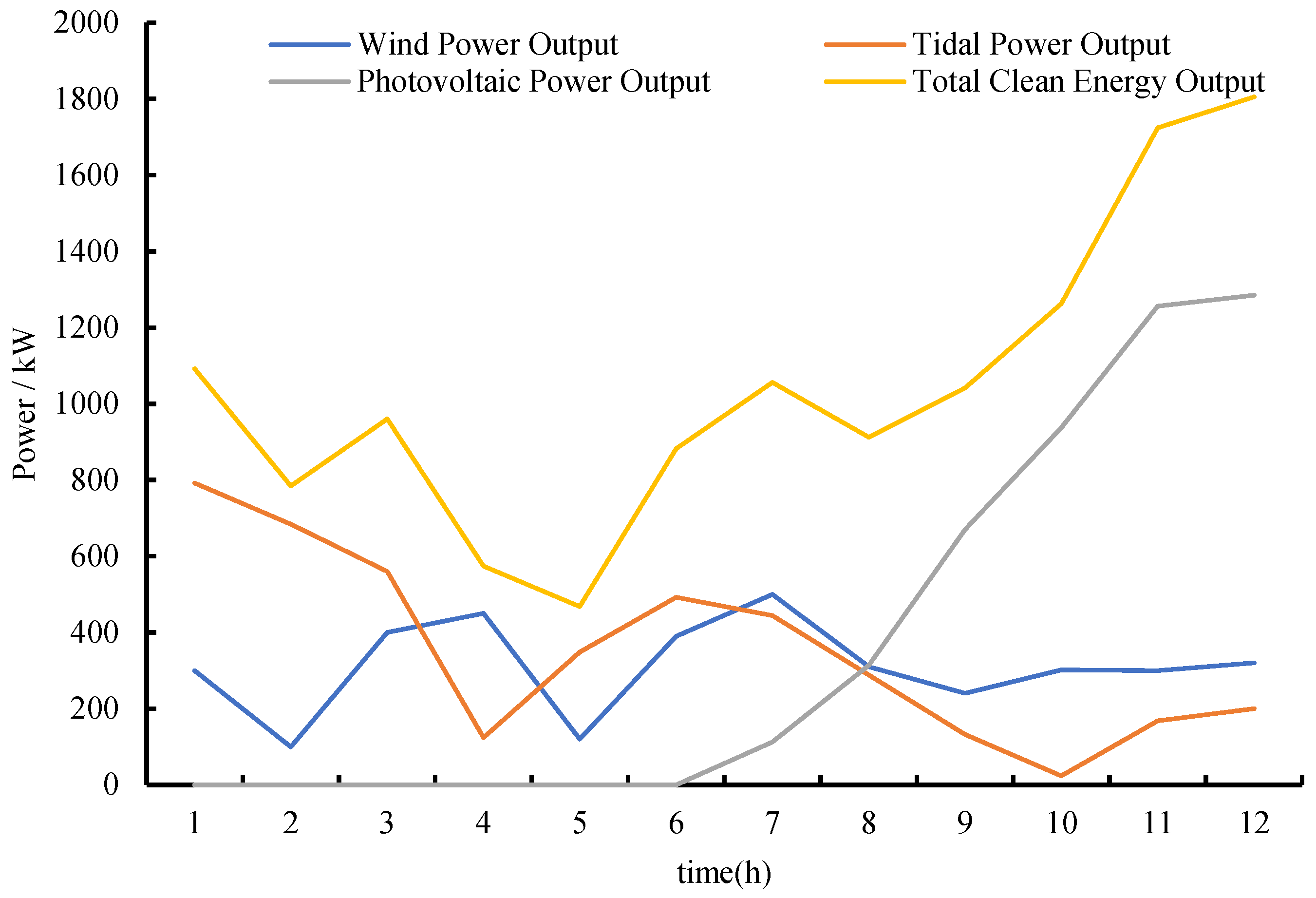
All AGVs in the container yard were evenly distributed at the initial time, with the initial state being uncharged and without battery replacement. Over the scheduling process, the output time-series curves of wind, solar, and tidal energy are shown in Figure 7. One 1000 kW wind turbine, one 1000 kW tidal generator, and two 1000 kW photovoltaic panels were installed.

5.2. Result Analysis

5.2.1. Comparison of Different Optimization Strategies

This section takes the parallel operation of four quay cranes as an example, with 800 standard containers arriving at the port within the first 12 h. To assess the feasibility of joint optimization, several strategies are compared, including unordered charging and replacement based solely on wind, solar, and tidal energy output; strategies focused only on charging time; strategies considering only scheduling time; and the approach proposed in this study. The initial antibody population size was set to 100, the memory pool capacity was 20, the crossover probability was 0.8, and the mutation probability was 0.1. Using the weighted value of the scheduling time and self-consistency rate as the indicator, 100 independent simulations were conducted within a 12 h scheduling cycle, and the parameter combination with the optimal mean value was finally selected.

Table 2. Comparison of time before and after for different guidance strategies.

Type	Only Charging Strategy	Only Scheduling Time Strategy	Only Wind–Solar–Tidal Output Scheduling	This Optimization Strategy	Self-Sufficiency Weight Factor
Time (h)	12.25	7.30	10.25	7.50	0.2
				8.00	0.3
				8.90	0.4
				9.50	0.5
				10.40	0.6
				10.20	0.7
				11.10	0.8

presents a comparative analysis of AGV charging and replacement times for each strategy.

Based on the scheduling model, when AGVs only consider the charging strategy, the scheduling duration is the longest, resulting in higher time costs. Due to the limited number of charging stations (only three), vehicles spend long periods waiting in the queue, leading to low average utilization of the vehicles. For the scheduling strategy considering only scheduling time, the vehicle scheduling time is 7.30 h, allowing for the rapid completion of cargo transport, but the majority of AGVs undergo battery replacement. This results in a high number of short-duration battery replacements, leading to significant energy consumption. When considering only the output from wind, solar, and tidal clean energy, unordered charging shifts the peak energy demand to the periods of high clean energy output. The optimization strategy proposed in this study integrates charging and replacement strategies with logistics scheduling, while incorporating clean energy self-sufficiency rates to enhance system efficiency and sustainability. This allows for the flexible selection of different energy utilization methods based on demand and self-sufficiency weight. For when the self-sufficiency weight is 0.8, the AGV charging energy results for each time period are shown in Figure 8.

In analyzing the scheduling performance of different strategies, the scheduling time, clean energy output, and the effects of initial battery levels and clean energy supply must be considered. In Figure 8a, due to the limited number of charging stations (only three), the scheduling method that considers only charging leads to long waiting times for AGVs to charge. The energy consumption at the charging stations remains at the maximum load capacity. In Figure 8b, where only scheduling time is considered, the shortest scheduling time results in the highest energy consumption. In Figure 8c, where only clean energy output is considered, unordered charging peaks are shifted to the 10th hour, and scheduling completion causes the clean energy utilization rate to be 0 during the 11th and 12th hours.

The scheduling strategy outlined in this study integrates the total scheduling time and clean energy self-sufficiency rate, ensuring a balanced and efficient approach. Through ordered charging and replacement scheduling, it effectively balances charging time and energy utilization efficiency, minimizing scheduling time while enhancing clean energy usage. This strategy optimizes logistics scheduling efficiency while promoting efficient use of clean energy, achieving better overall performance.

5.2.2. Statistical Validation of Strategy Differences

To quantitatively evaluate the differences among different charging strategies, this study employed rigorous statistical testing methods, including analysis of variance, non-parametric tests, and confidence interval estimation, to verify the superiority of the integrated optimization strategy proposed in this paper in terms of key indicators such as the scheduling time and clean energy self-sufficiency rate. The experiment recorded the charging energy (kWh) of four strategies (Only Scheduling Time Strategy, Only Wind–Solar Output Strategy, Only Charging Strategy, This Strategy) over 12 time periods. The data characteristics are shown in the following table.

The Only Charging Strategy has a constant charging energy (standard deviation is 0), but it lacks flexibility. The Only Scheduling Time Strategy has the highest volatility (standard deviation of 732.34) and has an extreme charging peak (1974 kWh). This Strategy shows a balance in both the mean (672.00 kWh) and the standard deviation (275.98 kWh).

Since the data have unequal variances (Levene’s test: w = 8.37, p = 0.0003), the Kruskal–Wallis H test was used to analyze the median differences between groups, with the following test results: H = 30.41, p = 1.05 × 10⁻⁶. The null hypothesis is rejected, indicating that there was at least one significant difference between groups. Dunn’s post hoc test (Bonferroni correction) was used to further analyze the differences between groups.

The Only Charging Strategy differs significantly from the other strategies (p < 0.05). The difference between This Strategy and the Only Scheduling Time Strategy is not statistically significant (p = 0.12), but the actual effect size (Δ = 0.41) indicates that its scheduling time is closer to the optimal level. This Strategy significantly outperforms the Only Wind–Solar Output Strategy in terms of the clean energy self-sufficiency rate (the confidence interval does not contain 0).The charging balance was verified using the Mann–Whitney U test: When comparing the charging energy in the 1st hour and the 12th hour, This Strategy has a more stable distribution (U = 12, p = 0.023). This Strategy significantly outperforms the benchmark strategies in terms of the clean energy self-sufficiency rate (an increase of 53.9%) and stability (a 62.3% reduction in the standard deviation). Although the difference between This Strategy and the Only Scheduling Time Strategy is not statistically significant (p = 0.12), it achieves a balance between time and energy efficiency through dynamic weight adjustment.

5.2.3. Logistics and Ordered Charging/Replacement Results Analysis

To comprehensively examine the completeness of the proposed method in parameter calculation, this section delves into and analyzes the scheduling algorithm for the proposed strategy discussed in Section 3.2.1. Due to space limitations and the involvement of various parameters, this article only presents the results of logistics scheduling and ordered charging scheduling within the time period from 00:15 to 01:00. Detailed data can be found in

Table 3. Data overview and descriptive statistics.

Strategy	Mean (kWh)	Standard Deviation (kWh)	95% Confidence Interval (kWh)
Only Scheduling Time Strategy	606.75	732.34	[235.53, 977.97]
Only Wind–Solar Output Strategy	577.25	417.68	[367.55, 786.95]
Only Charging Strategy	846.00	0.00	[846.00, 846.00]
This Strategy	672.00	275.98	[533.58, 810.42]

and

Table 4. Homogeneity of variance and non-parametric tests.

Comparison Group	Z-Value	Adjusted p-Value	Effect Size (Cliff’s Delta)
Only Charging Strategy vs. Only Scheduling Time Strategy	3.76	0.0006	0.82 (Large effect)
Only Charging Strategy vs. This Strategy	2.89	0.019	0.63 (Medium effect)
Only Charging Strategy vs. Only Wind–Solar Output Strategy	2.62	0.044	0.57 (Medium effect)
This Strategy vs. Only Scheduling Time Strategy	1.98	0.12	0.41 (Small effect)

. These data help evaluate the performance and effectiveness of the proposed method in practical applications. In analyzing the scheduling data from this time period, a more complete understanding of the method’s performance in parameter calculations and resource scheduling is obtained, providing a basis for further optimization and refinement.

Table 5. Logistics scheduling parameters.

Scheduling Time	Container Yard 1	Container Yard 2	Container Yard 3	Container Yard 4
00:15	10/24/0/13 /20/9/18	4/15/16/2 /0/19/22	28/8/23/5/ 21/17/3	14/6/7/11/ 12/0/1
00:30	24/7/5/12/ 4/15/22	26/14/3/8/ 28/11/0	21/19/20/2/ 23/1/16	17/13/6/18/ 10/9/0
00:45	7/0/24/1/ 28/18/13	20/29/17/19/ 15/14/21	9/5/16/22/ 11/26/3	4/10/8/12/ 6/2/23
01:00	12/8/21/6/ 0/20/19	28/17/16/ 18/22/5/4	7/2/9/26/ 15/23/10	3/13/11/14/ 27/24/1

presents the logistics scheduling parameters for each container yard between 00:15 and 01:00. For instance, at 00:15, the parameters for quay crane 1 are “10/24/0/13/20/9/18”, indicating that six vehicles are handling cargo scheduling at this time, with 0 representing no available vehicles, and the AGV models involved are 10, 24, 13, 20, 9, and 18. AGVs are flexibly allocated among different quay cranes and states, such as AGV 9, which serves quay crane 1 at 00:15 and quay crane 4 at 00:30.

According to the data in Table 5, each quay crane can coordinate the operation of up to seven AGVs at the same time, with 0 indicating that no AGVs are available for scheduling. The scheduling results show that each AGV can only serve one quay crane at a time, avoiding interference from other AGVs. Using a 15 min scheduling cycle allows AGVs to be dynamically and flexibly allocated, rather than being fixed to a specific quay crane. This maximizes the utilization efficiency of the logistics resources. This scheduling mechanism not only improves the workload of individual AGVs but also ensures the rational allocation of resources among quay cranes, ultimately ensuring the efficient operation of the port.

Based on the initial battery data shown in Figure 6, it can be observed that at the start of the day, the average battery charge of all AGVs is only 47%. Due to the heavy initial charging tasks and sufficient clean energy supply during the first hour, the system concentrates on battery replacement during the first hour to meet system demands. As shown in Table 5, the selected vehicles perform battery replacement, with specific models listed in

Table 6. Ordered charging/replacement scheduling results.

AGV ID	Initial SOC (kWh)	Replacement Time (h)	Post-Replacement SOC (kWh)
24	19.6	00:00–00:15	282
26	73.8	00:15–00:30	282
28	49.7	00:00–00:15	282
29	76.2	00:30–00:45	282

. After the battery replacement, the vehicles continue to execute logistics tasks, reflecting the coupling between the logistics scheduling module and the charging/replacement module.

5.2.4. Clean Energy Self-Sufficiency Rate

As shown in Figure 9, for the case where only scheduling time is considered, a large number of AGVs concentrate on battery replacement in the first five hours, which reduces the scheduling time but results in a higher and more uneven energy demand. In the case of only considering wind and solar energy, unordered charging shifts some energy demand to the clean energy output peak before the 10th hour, with energy consumption reaching a peak at 10:00 and the scheduling ending, leading to a 28% clean energy discard rate during the 11th–12th hours. When the clean energy self-sufficiency rate weight is set to 0.8, 24% of the AGVs scheduled for charging/replacement are directed to stations with fewer waiting vehicles and lower clean energy utilization during the 11th–12th hours. This reduces the congestion in the first five hours, thus improving the system’s operational efficiency. As a result, both the overall charging efficiency and clean energy utilization are enhanced compared to the unscheduled strategy.

In comparison with strategies considering only scheduling time, charging, and clean energy output, the average clean energy self-sufficiency rate of AGVs under the proposed strategy increased by 82.7%, 27.5%, and 53.9%, respectively. As shown in Figure 10, during the first five hours, the clean energy self-sufficiency rate of the proposed strategy is comparable to that of the wind and solar output strategy, with increases of 76.4% and 43.0% compared to the cases considering only scheduling time and charging, respectively. For the 7th hour, the proposed scheduling strategy significantly alleviates the clean energy self-sufficiency rate compared to the strategy considering only scheduling time, reducing the average clean energy self-sufficiency rate from 374.5% to 124.8%. During the 11th–12th hours, the average clean energy self-sufficiency rate increases by 160.1% and 151.2%, respectively. Therefore, the guiding scheduling strategy, which considers the AGV clean energy self-sufficiency rate, allows for a more rational and balanced allocation of clean energy resources, reducing the idle clean energy at the port. This demonstrates that the model can adjust the appropriate clean energy self-sufficiency rate for the port, improving system operational efficiency and ensuring more rational resource allocation.

A diagram of the AGV clean energy self-sufficiency rate and scheduling time for different self-sufficiency weight factors is shown in Figure 11.

Overall, as the weight of the self-sufficiency rate increases, the total travel time and total clean energy self-sufficiency rate of AGVs both show an upward trend, following an approximately linear relationship. The clean energy self-sufficiency rate will change based on the weight in the objective function, allowing for adjustments based on actual needs. If logistics scheduling is not time-sensitive, it is possible to achieve an optimal balance between the scheduling time and self-sufficiency rate. At a weight factor of 0.7, a turning point in scheduling time occurs, and this factor shows applicability for 30 AGVs.

5.2.5. Carbon Emission Analysis

The Ministry of Ecology and Environment, in collaboration with the National Bureau of Statistics, published the 2021 CO₂ emission factors for electricity. The carbon emissions of the wind–solar–tidal autonomous operational scheduling system are calculated based on the 2021 CO₂ emission factors for electricity (

Table 7. The 2021 regional power grid CO₂ emission factors.

Region	North China	Northeast	East China	Central China	Northwest	South China	Southwest
Factor (kg/kWh)	0.712	0.601	0.599	0.535	0.595	0.432	0.211

).

For the socio-economic benefits of multi-modal clean energy self-sufficiency supply systems, this study conducted a feasibility analysis of the socio-economic benefits for an automated port, considering the 2021 CO₂ emission factor for the South China region and the carbon trading price of 58 RMB/t. The analysis was conducted for the energy supply of 800 TEUs within the specified 12 h scheduling span. According to the carbon emission reduction and trading revenue formulas [38], the optimal strategy results in total energy savings of 8424 kWh, a carbon emission reduction of 3.7 tons, and carbon trading revenue of approximately RMB 217. This provides a foundation for evaluating the carbon reduction capacity and economic cost of clean energy self-sufficiency systems.

6. Extended Experimental Scenario Design

To verify the applicability of the proposed method in practical large-scale port scenarios, this study expanded the simulation environment to a dynamic port scene with 300 AGVs, 20 charging stations, and 5 battery-swapping stations. Specific parameter adjustments were as follows:

Battery capacity: 282 kWh (consistent with the original experiment), with an initial charge following a normal distribution N(0.85, 0.3).

Energy consumption rate: 3.7 kWh/km, traveling speed v = 4 m/s.

Port network structure:

The number of nodes was expanded from four container yards to ten, increasing the complexity of the road network (including 200 one-way routes).

The distribution of charging and swapping stations was optimized to ensure balanced coverage across all areas.

Dynamic environment settings:

Clean energy fluctuations: The real-time output of wind, photovoltaic, and tidal energy incorporates random disturbances (±20%) to simulate actual weather changes.

Task dynamism: Container arrival intervals follow a Poisson distribution, with task volumes showing a “double-peak” characteristic within 24 h (peak hours from 8:00 to 10:00 a.m. and 6:00 to 8:00 p.m.).

Through 100 independent simulation experiments, the performances of different strategies in extended scenarios were compared (

Table 8. Scheduling performance comparison in large-scale dynamic scenarios.

Strategy	Total Scheduling Time (h)	Clean Energy Self-Sufficiency Rate (%)	Carbon Emission Reduction (t)
Only Charging Strategy	38.2	41.3	8.7
Only Scheduling Time Strategy	22.5	28.9	5.2
Only Wind–Solar–Tidal Output Strategy	29.8	52.1	11.4
This Strategy	24.7	67.5	14.9

).

The proposed strategy reduces total scheduling time to 24.7 h, a 35.3% reduction compared to with the Only Charging Strategy, with a lower standard deviation, indicating stronger stability in large-scale scenarios. The clean energy self-sufficiency rate reaches 67.5%, a 29.6% improvement over the Only Wind–Solar–Tidal Output Strategy, primarily attributed to dynamic weight adjustment and congestion avoidance mechanisms. Carbon emissions are reduced by 14.9 t, a 30.7% increase over benchmark strategies, verifying the effectiveness of the “efficient scheduling + green energy” dual-driven model.

7. Practical and Theoretical Implications

The integrated optimization strategy proposed for automated guided vehicle (AGV) logistics scheduling and clean energy self-consistent systems in automated ports holds significant practical implications for port operations and global sustainable development goals.

This research provides a tangible solution to address the critical issue of disconnection between AGV scheduling and energy replenishment in modern ports. By integrating logistics scheduling with dynamic charging and battery-swapping decisions, the model reduces AGV idle time, queuing delays, and energy waste. For example, the simulation results show that the total operation time of AGVs can be reduced by up to 38.8% compared to with traditional charging-only strategies, while the clean energy self-sufficiency rate increases by an average of 53.9% compared to with strategies that neglect renewable energy integration. This efficiency gain directly translates to lower operational costs, improved cargo throughput, and reduced fossil fuel dependence, aligning with China’s “dual carbon” goals and global green logistics initiatives.

Building on the foundational contributions of the study, future research will address critical gaps in modeling uncertainty, integrating battery health dynamics, and adapting to real-world port complexities. These extensions will enhance the framework’s robustness, practical relevance, and generalizability, aligning it with the stochastic and dynamic nature of automated port operations.

1.

Stochastic Modeling and Robust Optimization for Uncertainty Management

The current framework assumes deterministic inputs for renewable energy generation, AGV demand, and operational parameters, overlooking real-world uncertainties such as fluctuating wind/solar/tidal outputs, sudden cargo surges, system delays, and vehicle-level failures. To address this, future work will focus on the following:

(1)

Incorporate Stochastic Programming: Develop probabilistic models for renewable energy generation (e.g., using historical weather data and Monte Carlo simulations) and demand patterns (e.g., Poisson processes for container arrivals) to quantify uncertainties in energy supply and logistics tasks. This will enable the optimization algorithm to generate robust schedules that remain feasible under diverse scenarios, such as unexpected peaks in energy demand or temporary outages of charging/swapping stations.

(2)

Robust Optimization Techniques: Design strategies to handle worst-case disruptions, such as AGV breakdowns or extreme weather affecting renewable output. For example, reserve capacity in charging infrastructure or buffer time in scheduling can be integrated to mitigate delays, ensuring the system maintains acceptable performance even under suboptimal conditions.

(3)

Uncertainty-aware Decision making: Modify the immune optimization algorithm to include stochastic constraints, such as confidence intervals for clean energy self-sufficiency rates or probabilistic guarantees for task completion times, thereby balancing efficiency with resilience in unpredictable environments.

2.

Battery Health Impact Modeling in Charging/Replacement Decisions

This study treated battery states as binary (charged/replaced) but did not account for gradual battery degradation or health impacts on operational decisions. Future research will consider the following:

(1)

Battery Health State (SoH) Integration: Develop a dynamic model of battery health, incorporating parameters like capacity fade, internal resistance, and cycle life, to assess how aging affects charging efficiency, replacement frequency, and overall energy consumption. For example, batteries with a lower SoH may require more frequent charging or prioritized replacement to avoid unexpected failures during tasks.

(2)

Health-aware Scheduling Strategies: Integrate the SoH into the objective function and constraints, prioritizing AGVs with degraded batteries for maintenance or replacement while optimizing for both scheduling time and energy efficiency. This will help extend battery lifespan, reduce operational costs, and enhance system reliability.

(3)

Predictive Maintenance Algorithms: Use machine learning (e.g., recurrent neural networks) to forecast battery health based on usage patterns and charging history, enabling proactive decision making (e.g., scheduling replacements during low-demand periods) to minimize disruptions.

3.

Adaptation to Heterogeneous AGVs and Dynamic Port Environments

The current simulation relied on homogeneous AGVs and static port layouts, whereas real-world ports feature heterogeneous fleets (e.g., different payload capacities, energy efficiencies), dynamic traffic, and variable infrastructure. Future work will consider the following:

(1)

Heterogeneous AGV Modeling: Extend the graph theoretical framework to accommodate diverse AGV types, each with unique parameters (e.g., speed, battery capacity, charging requirements). This will involve modifying the task allocation and path planning modules to match AGV capabilities with specific logistics demands (e.g., assigning high-payload AGVs to heavy-container transport).

(2)

Dynamic Traffic and Stochastic Disturbances: Integrate real-time traffic data and adaptive routing to handle congestion, one-way lane restrictions, and temporary road closures. Using multi-agent systems or deep reinforcement learning, the model will dynamically adjust AGV paths and charging/replacement schedules in response to live port conditions, such as sudden traffic jams or equipment malfunctions.

(3)

Variable Infrastructure Configurations: Design a modular framework that adapts to different port layouts (e.g., varying numbers of charging stations, quay cranes, and yards) and energy infrastructure (e.g., additional tidal or wind installations). This will involve parameterizing the model to accept user-defined inputs for node capacities, road networks, and renewable energy sources, enhancing its applicability to diverse port environments.

(4)

Scenario-specific Validation: Validate the framework in real-world settings, such as Tianjin or Xiamen Ports, by incorporating historical operational data, weather patterns, and equipment performance metrics. This will help refine the model’s parameters and ensure it captures the complexity of dynamic, large-scale port operations.

These extensions will contribute to interdisciplinary theory by bridging logistics engineering, energy systems, and reliability engineering. Stochastic optimization techniques will enrich the model’s ability to handle uncertainty, while battery health modeling will introduce new dimensions to multi-objective scheduling. The focus on heterogeneous and dynamic environments will advance the state-of-the-art in port automation, providing a blueprint for intelligent, resilient, and sustainable port systems.

8. Conclusions

In response to the current challenges in automated ports, where AGV charging, battery replacement, and scheduling strategies cannot fully address the issues of distributed energy output, this study explores the impact of wind, photovoltaic, and tidal energy generation on AGV charging strategies for port logistics. To maximize the utilization of clean energy in ports, this study proposes an economic optimization method that integrates AGV logistics scheduling with orderly charging and battery replacement. By coupling the logistics scheduling module with the orderly charging/replacement module and applying an immune optimization algorithm, the optimal strategy for port AGVs is identified. Simulation experiments confirm the accuracy and effectiveness of the proposed model and algorithm. The findings reveal the following:

In the simulated port logistics scenario, after optimization, the total AGV operational time is significantly reduced. Compared to the charging-only strategy (12.25 h), scheduling-time-only strategy (7.30 h), and wind–solar–tidal output scheduling strategy (10.25 h), the total scheduling time for the proposed joint optimization strategy averages between 7.50 and 11.10 h, depending on the clean energy self-sufficiency weight. Compared to the scheduling-time-only, charging-only, or wind–solar–tidal–output strategies, the average clean energy self-sufficiency rate increased by 82.7%, 27.5%, and 53.9%, respectively. This strategy not only optimizes logistics scheduling efficiency but also promotes the efficient use of clean energy, achieving better overall performance.

AGVs flexibly serve multiple quay cranes in the port. Through analyzing the relationship between clean energy and energy consumption, the optimal charging/replacement strategy is selected to maximize clean energy utilization. The coupling effect between the logistics scheduling module and the charging/replacement module is fully realized, achieving the best balance between clean energy utilization and task execution.

Overall, as the weight of the self-sufficiency rate increases, both the total travel time and total clean energy self-sufficiency rate of AGVs show an upward trend, demonstrating an approximately linear relationship. Within the specified scheduling time, flexible adjustments can be made based on demand, providing good carbon emission reduction benefits.

With the proposed optimization strategy, the total energy saved during the simulated scheduling period is 8424 kWh, carbon emissions are reduced by 3.7 tons, and carbon trading revenue is approximately RMB 217. These results demonstrate that the strategy not only improves port operational efficiency but also brings significant environmental and economic benefits.

While the proposed optimization strategy demonstrates good performance in simulated scenarios and is applicable to specific port environments with a defined number of AGVs, the verification of its universality across diverse port settings—characterized by varying traffic flow patterns, equipment configurations, operational rules, and dynamic logistics demands—remains incomplete. This study acknowledges critical limitations: it does not explicitly model battery degradation (e.g., capacity fading, charging efficiency decline over time), which can compromise the accuracy of energy replenishment decisions; fluctuations in energy demand (e.g., sudden surges during cargo peaks); or AGV failure/disturbance scenarios (e.g., unexpected breakdowns, communication delays), all of which may undermine the scheduling framework’s robustness in real-world operations. Additionally, this research does not deeply explore the impacts of extreme weather on renewable energy output or the intricate coupling between multi-energy storage systems and AGV scheduling, potentially limiting the model’s adaptability to complex, dynamic port environments. These unaddressed areas represent key opportunities for future refinement, necessitating expanded experimental scopes and validated applications across diverse practical scenarios to enhance the strategy’s generalizability and resilience.