Data-Driven Distributionally Robust Collaborative Optimization Operation Strategy for Multi-Integrated Energy Systems Considers Energy Trading

Abstract

The strong uncertainty of renewable energy poses significant reliability and safety challenges for the coordinated operation of multi-integrated energy systems (MIES). To address this, a data-driven two-stage distributed robust collaborative optimization scheduling model for MIES is proposed, based on a spatiotemporal fusion conditional diffusion model (STF-CDM). First, to more accurately capture the uncertainty in renewable energy output, the model utilizes a scenario set generated by the STF-CDM model and reduced via the K-means clustering algorithm as the initial renewable energy scenarios for the distributed robust optimization set. The STF-CDM model employs a Temporal module component (TMC) unit composed of Transformer time-series modules and a Spatial module component (SMC) unit composed of CNN neural networks for feature extraction and fusion of time-series and spatial-series data. Second, a benefit allocation method based on multi-energy trading contribution rates is proposed to achieve equitable distribution of cooperative gains. Finally, to protect participant privacy and enhance computational efficiency, an alternating direction multiplier method (ADMM) coupled with parallelizable column and constraint generation (C&CG) is employed to solve the energy trading problem. The case analysis results demonstrate that the STF-CDM model proposed in this study exhibits superior performance in addressing the uncertainty of renewable energy output. Concurrently, the asymmetric Nash game mechanism and the ADMM-C&CG solution algorithm proposed in this study achieve a fair and reasonable distribution of benefits among all participants when handling energy transactions and cooperative gains. This is accomplished while ensuring system robustness, economic efficiency, and privacy.

1. Introduction

Multi-integrated energy systems (MIES) serve as a core technological pathway for achieving the dual carbon goals [1]. By integrating electricity, heat, cooling, and gas multi-energy flow subsystems and coordinating multiple stakeholders including governments, energy suppliers, and users, they significantly enhance energy utilization efficiency and renewable energy absorption capacity [2]. However, as renewable energy penetration continues to rise, its inherent intermittency and volatility pose severe challenges to multi-agent collaborative optimization scheduling [3]. These challenges primarily manifest as increased difficulty in matching supply and demand, higher operational costs, and greater complexity in carbon emission control. Traditional single integrated energy systems struggle to independently address these challenges due to scale limitations and insufficient disturbance resilience [4]. In contrast, MIES establishes a peer-to-peer (P2P) energy exchange architecture through public coupling points, enabling intelligent coordination and flexible transactions between IES. This facilitates broader resource optimization and reduces societal costs. Nevertheless, the integration of high proportions of renewable energy introduces significant uncertainty into the system, necessitating the development of more advanced optimization scheduling methods [5].

To address uncertainty, stochastic optimization (SO) and robust optimization (RO) represent two traditional approaches [6]. The SO relies on probability density functions for uncertain parameters, generating dispatch strategies through scenario sampling. However, its computational efficiency declines sharply with increasing scenario scale, and the precision of probability distributions is difficult to guarantee, leading to reduced decision reliability [7]. The RO requires only information about the fluctuation range of uncertainty sets, without needing probability models. Yet its tendency to optimize for worst-case scenarios often results in overly conservative solutions with poor economic performance [8]. Distributionally Robust Optimization (DRO), as an emerging approach, combines the strengths of SO and RO: it constructs probabilistic fuzzy sets in a data-driven manner and makes decisions based on the worst-case distribution. probability of strong assumptions about the probability distribution type while reducing conservatism. Common methods for constructing fuzzy sets include those based on probability distances (e.g., Wasserstein distance) and moment information. Numerous studies have already been conducted in this area. Ma et al. [9] develop a two-stage DRO model to coordinately optimize a port-integrated energy system and berth allocation under dual uncertainties of wind power and ship arrivals, demonstrating improved economic and environmental performance while effectively hedging against risks. Song et al. [10] explored sustainable operation strategies for CCUS units under a low-carbon economy using a two-layer DRO model. Rauf et al. [11] propose a DRO model with a linear decision rule for unit commitment and optimal battery energy storage system (BESS) sizing in a renewable-integrated distribution network, achieving minimized operational costs and enhanced scheduling efficiency under renewable and load uncertainties. Shen et al. [12] develop a Wasserstein metric-based DRO bidding model for IES in spot electricity markets, effectively managing price uncertainty to minimize expected cost and risk while demonstrating superior out-of-sample performance compared to stochastic programming and robust optimization. Shi et al. [13] propose an adaptive step-size distributed optimization method based on ADMM for a multi-microgrid integrated energy system (MMIES), incorporating energy storage coordination and carbon management strategies to enhance economic and environmental benefits while preserving operational privacy. Zhou et al. [14] propose a two-stage distributionally robust optimization (DRO) model that separately models source-side and load-side uncertainties using DRO and scenario-based stochastic programming, respectively, resulting in a more economical and reliable scheduling plan that saves an average of 11% in cost compared to traditional methods. Ma et al. [15] propose a data-driven distributionally robust optimization (DRO) model for an electric-thermal-hydrogen integrated energy system, using CGAN-generated scenarios and a comprehensive norm-based uncertainty set to reduce operating costs by 2.1% compared to traditional robust optimization while maintaining computational efficiency. However, these methods typically require converting to convex optimization problems using skewed linear decision rules and duality theorems. The introduction of 0–1 variables often increases model complexity and computational difficulty (NP-hard problems). In contrast, the data-driven DRO method employing 1-norm and ∞-norm constrained composite norm fuzzy sets can process typical scenario probability distributions through parallel solving. This approach effectively avoids duality derivation and the introduction of integer variables, significantly enhancing solution efficiency.

In renewable energy scenario generation, traditional methods like Monte Carlo sampling, probability density methods, Markov chains, and time series approaches primarily rely on statistical learning models. These determine parameters based on historical data and generate scenarios through sampling. However, these methods struggle to fully capture the spatiotemporal correlations of wind and solar power output and other unknown information, lacking universal applicability in complex real-world scenarios.

In recent years, artificial intelligence technologies have demonstrated significant potential in renewable energy scenario generation, gradually replacing traditional statistical methods. Diffusion models, as a new class of deep generative models, have gained widespread application in wind and solar power scenario modeling due to their stable training process, robust distribution fitting capabilities, and diverse generated samples. Compared to generative adversarial networks (GANs) that require adversarial training, diffusion models significantly enhance their ability to capture complex probabilistic structures by defining forward noise addition and backward denoising processes [16]. They demonstrate advantages in generating high-dimensional spatiotemporal sequences. Diffusion models do not rely on prior distribution assumptions and can autonomously learn the stochastic characteristics of renewable energy output from historical data, thereby substantially improving the system’s management capabilities in addressing future uncertainties. In practical applications for generating renewable energy scenarios, diffusion models iteratively produce scenario sets that match actual wind and solar output distributions through denoising. Concurrently, conditional control within diffusion models is typically achieved via cross-attention mechanisms or conditional encoding injections, enabling flexible adaptation to diverse generation tasks—including extreme event construction, few-shot generalization, and even zero-shot novel pattern generation. Diffusion models have seen extensive application in the generation of renewable energy scenarios: Liang et al. [17] develops a modified airtightness calculation model for compressed air energy storage (CAES) caverns based on the solution-diffusion model, demonstrating that it more accurately characterizes air permeation in rubber seals compared to the traditional pore-flow model, which overestimates leakage by 225%. Zhao et al. [18] proposes a conditional diffusion model (CDSG) for generating realistic and diverse joint source-load scenarios in deep decarbonized power systems, effectively capturing complex spatial-temporal correlations and improving dispatch feasibility compared to existing methods. Zhao et al. [19] proposes a hierarchical multi-agent deep reinforcement learning (MADRL) method integrated with discrete diffusion models, named gMADRL-VCS, to optimize energy-efficient and cooperative navigation and sensing strategies for unmanned vehicles in ground-air-space communication systems, demonstrating superior performance in data collection and energy savings across real-world scenarios.

However, despite significant advances in generative quality, diffusion models exhibit critical shortcomings in constructing conditional noise networks. Current approaches predominantly employ fully connected networks or simple encoder structures for conditional injection, lacking systematic integration of spatiotemporal feature extraction and prediction. This results in insufficient accuracy and limited generalization when modeling cross-regional correlations, complex weather pattern responses, and multi-energy coupling dynamics. Therefore, there is an urgent need to develop a conditional diffusion architecture that integrates spatial-temporal inductive biases to enhance the physical consistency and system operability of generated scenarios.

On the other hand, with the development of the electricity market, each IES within the MIES belongs to different stakeholders. Establishing an appropriate benefit distribution mechanism to promote the sustainable and coordinated optimization operation of the MIES is crucial. Cooperative games are considered an effective means to address benefit distribution issues. Chen et al. [20] proposed independent and cooperative operation models for participants in industrial park integrated energy systems, employing the Shapley value method to allocate cooperative benefits. Amiri et al. [21] develops a machine learning model to forecast neighborhood-level building energy use and employs SHAP analysis to identify key influencing factors, such as building size and type, providing a data-driven tool for urban sustainability planning. Lu et al. [22] develops an improved Shapley Value method for multi-park integrated energy systems that coordinates renewable energy uncertainty, carbon emissions, and demand response to achieve low-carbon operation and fair benefit allocation among the participants. Abdollahi et al. [23] proposes a framework for intraday regional flexibility markets managed by Advanced Virtual Power Plants (AVPPs). Through an innovative hierarchical market clearing mechanism and a two-stage optimization model, this framework effectively integrates distributed energy resources into trading. It enhances AVPP economic returns by 28% while reducing short-term load fluctuations in distribution grids by 35%, achieving synergistic optimization of energy trading efficiency and system operational stability. Song et al. [24] develops highly accurate XGBoost models for solar radiation estimation in China and, most importantly, uses the SHAP method to provide comprehensive global and local explanations of the model’s predictions, thereby enhancing its interpretability and transparency. However, the Shapley method only considers marginal contributions for benefit distribution, failing to guarantee global benefit maximization. Nash bargaining, which accounts for participants’ interests, strategies, and information, has gained significant attention in recent years due to its superior handling of non-independence and interactivity among participants compared to the Shapley value method [25]. To overcome the drawback of equal distribution in traditional Nash bargaining, asymmetric allocation strategies by assigning different bargaining powers have also been explored. Chen et al. [26] develops a cooperative framework for multi-agent integrated energy systems, using Nash bargaining to ensure fair benefit allocation and coordinated operation among participants, thereby improving economic efficiency and system flexibility. Huang et al. [27] develops a cooperative framework for multiple building integrated energy systems using a multi-agent deep reinforcement learning approach for operational optimization and a Nash-Harsanyi bargaining model for fair cost allocation, effectively reducing both operational costs and carbon emissions. Zhang et al. [28] proposes a two-stage cooperative optimization strategy based on Nash bargaining theory for microgrids and shared energy storage systems to achieve voltage regulation in distribution networks while ensuring fair benefit sharing among participants. Zhu et al. [29] proposes an asymmetric Nash bargaining-based energy sharing strategy for integrated energy service providers, using a nonlinear mapping function to fairly allocate benefits and incentivize cooperation, thereby enhancing renewable energy utilization and reducing carbon emissions. However, the benefit allocation processes in the literature did not consider contributions from energy transactions other than electricity.

Table 1. A comparative summary of this study and existing studies.

References	Optimization Model	Data-Driven	Cooperative Benefits	Energy Trading
[30]	RO	×	√	×
[8]	RO	×	×	√
[22]	SO	×	×	√
[14]	SO	×	√	×
[26]	DRO	×	√	√
[27]	DRO	×	√	×
[25]	DRO	√	×	√
[31]	DRO	√	√	×
This study	DRO	√	√	√

shows the comparative summary of this study and existing studies.

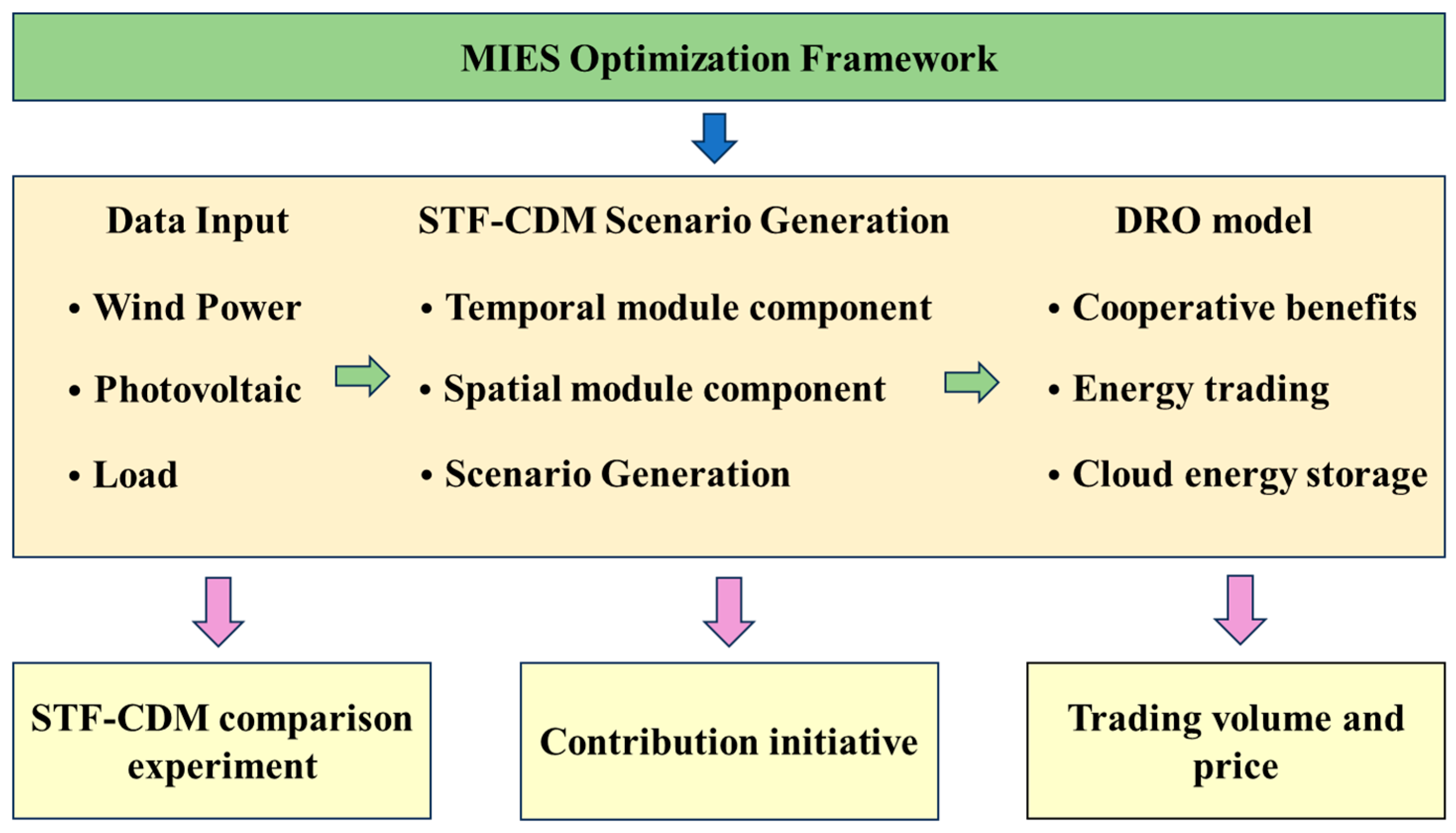
Despite progress in DRO and scenario generation, MIES collaborative optimization still faces following challenges: (1) Spatiotemporal uncertainty of high renewable energy penetration is difficult to accurately characterize; (2) Revenue distribution mechanisms in multi-energy transactions remain imperfect; (3) Existing methods struggle to balance privacy protection and computational efficiency. Against the backdrop of energy conservation and emission reduction targets, these issues pose challenges to the economic and secure operation of MIES and require urgent resolution. Based on the above research and gap, this article proposes a data-driven two-stage distributed robust collaborative optimization scheduling model for MIES based on a spatial-temporal fusion based conditional diffusion model. The optimization framework of this study is shown in Figure 1. Compared to existing research, the innovation of this work lies in the first application of a spatiotemporal fusion conditional diffusion model to MIES scenario generation. Combined with a multi-energy transaction contribution rate design for the revenue distribution mechanism, it addresses the limitations of existing methods that cannot simultaneously ensure both scenario quality and revenue fairness. The main innovations and contributions of this research are as follows:

(a)

To more accurately describe the stochastic characteristics of renewable energy, a spatial temporal fusion conditional diffusion model is proposed for generating photovoltaic and wind power scenarios in MIES, constructing the initial renewable energy scenarios for the DRO set. This method is intended to integrate Transformer and CNN modules into the traditional diffusion model, enabling the extraction of spatiotemporal features from scenario data to ensure the accuracy of generated scenarios.

(b)

Based on the contribution rates of each IES, an asymmetric Nash bargaining mechanism grounded in P2P electrothermal multi-energy transaction contribution rates are proposed to allocate cooperative benefits among IESs, ensuring the fairness and rationality of surplus distribution.

(c)

To enhance model solution efficiency and effectively protect the privacy of all parties, we propose a distributed solution for energy trading problems using an ADMM coupled with parallelizable C&CG.

(d)

Establish a comprehensive MIES collaborative optimization framework to provide new insights for high-penetration renewable energy systems during energy planning transitions.

2. Multi-Integrated Energy Systems (MIES) Framework and Model

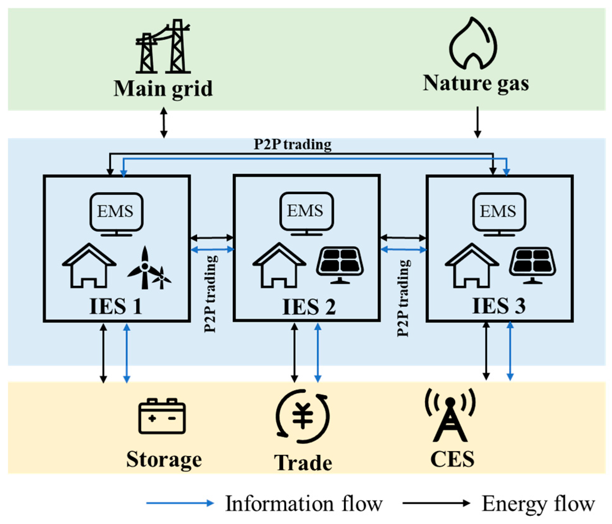
The schematic of the MIES operational model framework proposed in this study is shown in Figure 2. IESs are directly connected to the upper-level energy grid, enabling them to purchase energy at prices set by the upper-level grid or engage in peer-to-peer (P2P) transactions among IESs through cooperative alliances. IES operators negotiate to exchange electricity and thermal energy based on their supply and demand needs, reducing reliance on the upper-level grid to lower operational costs. Concurrently, collaborating IES operators reduce substantial investment costs for internal energy storage systems by leasing cloud energy storage (CES), thereby promoting renewable energy integration. Additionally, each IES is equipped with an energy management system (EMS). Advanced 5G communication technology enables real-time energy exchange and price transmission between IES, ensuring high efficiency while safeguarding IES privacy requirements.

2.1. Internal System Model of IES

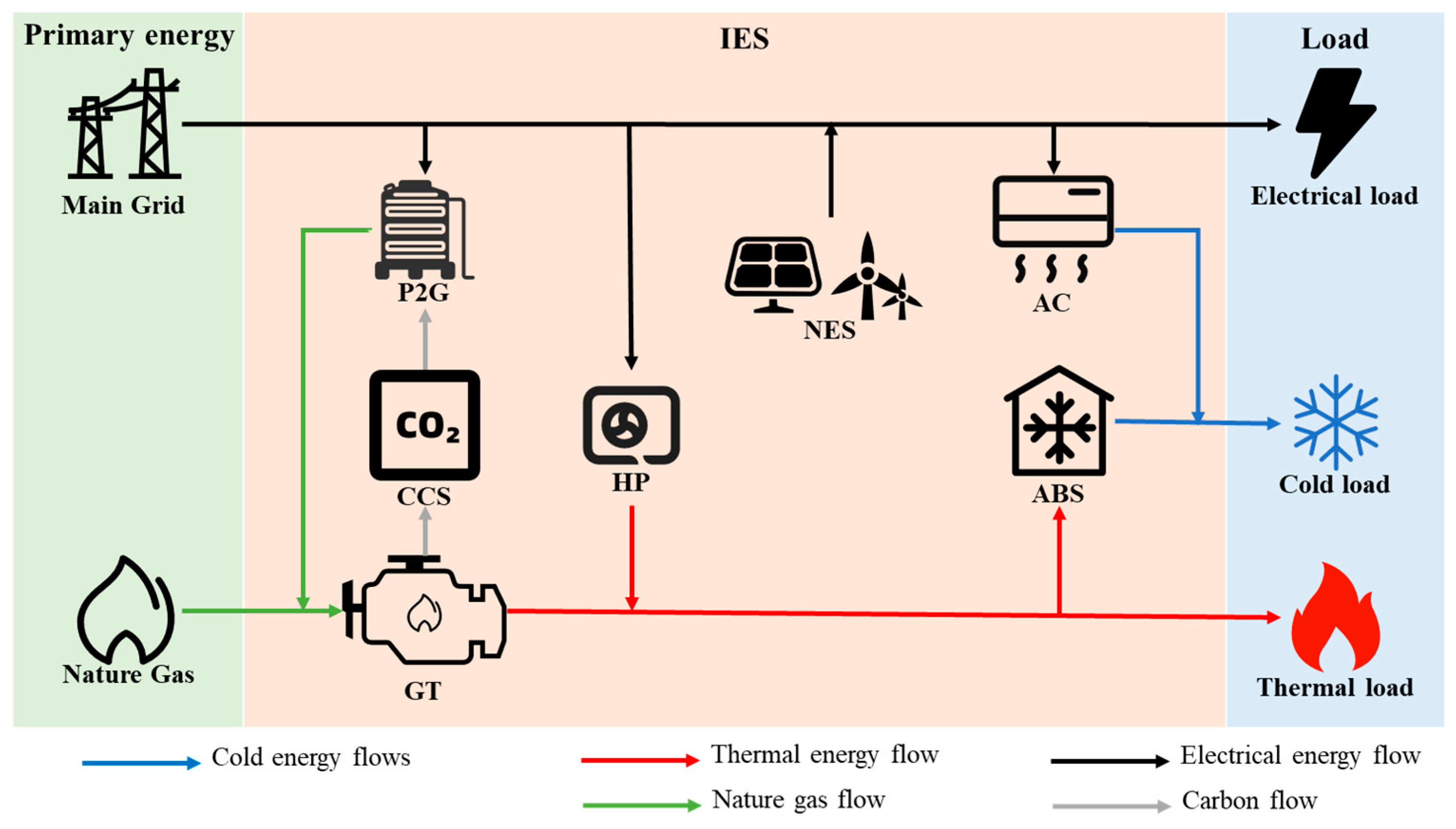
Extensive research exists on modeling multi-energy coupling systems. Ahmad et al. [32] conducted a thermodynamic analysis of solar trigeneration systems, while Bagherian et al. [33] comprehensively reviewed optimization techniques for CHP and CCHP systems. Building upon these works, this study constructs equipment models suitable for the coordinated optimization of MIES. An internal system model of the IES, which selects appropriate distributed generation sources based on its geographical location and other conditions is shown in Figure 3. To better achieve multi-energy utilization, energy coupling equipment such as GT, HP, AC, and EC are integrated. P2G and CCS conversion equipment are introduced to reduce CO₂ emissions. Concurrently, flexible loads are considered to further facilitate renewable energy integration and enhance user participation. Some models in this paper are derived from References [15,18,25].

GT generates electrical and thermal energy by burning natural gas, with their output models and constraints defined as shown in Equation (1).

$$\left\{\begin{array}{l}{P}_{i,\mathrm{e},t}^{\mathrm{GT}}={\eta }_{\mathrm{GT},\mathrm{e}}{H}_{\mathrm{GHV}}{G}_{i,t}^{\mathrm{GT}}\hfill \\ P_{i,\mathrm{h},t}^{\mathrm{GT}}={\eta }_{\mathrm{GT},\mathrm{h}}{H}_{\mathrm{GHV}}{G}_{i,t}^{\mathrm{GT}}\hfill \\ 0⩽P_{i,\mathrm{e},t}^{\mathrm{GT}}⩽P_{i,\mathrm{e},\max }^{\mathrm{GT}}\hfill \\ 0⩽P_{i,\mathrm{h},t}^{\mathrm{GT}}⩽P_{i,\mathrm{h},\max }^{\mathrm{GT}}\hfill \end{array}\right.$$

(1)

where $P_{i,\mathrm{e},t}^{\mathrm{GT}}$ and $P_{i,\mathrm{h},t}^{\mathrm{GT}}$ represent the electrical power output and thermal power output of the gas turbine, respectively; ${\eta }_{\mathrm{GT},\mathrm{e}}$ and ${\eta }_{\mathrm{GT},\mathrm{h}}$ denote the electrical efficiency and thermal efficiency of the gas turbine, respectively; $P_{i,\mathrm{e},\max }^{\mathrm{GT}}$ and $P_{i,\mathrm{h},\max }^{\mathrm{GT}}$ denote the maximum electrical power output and maximum thermal power output of the gas turbine, respectively.

As an efficient device utilizing low-grade thermal energy, HP are crucial low-carbon energy-saving equipment in IES. Driven by electrical power, the relationship between the HP’s heating power output and its electricity consumption is as shown in Equations (2) and (3).

$$P_{i,\mathrm{h},t}^{\mathrm{HP}}={\eta }_{\mathrm{HP}}{P}_{i,\mathrm{e},t}^{\mathrm{HP}}$$

(2)

$$0⩽P_{i,\mathrm{h},t}^{\mathrm{HP}}⩽P_{i,\mathrm{h},\max }^{\mathrm{HP}}$$

(3)

where ${\eta }_{\mathrm{HP}}$ denotes the heating performance factor of the HP; $P_{i,\mathrm{h},\max }^{\mathrm{HP}}$ represents the maximum heating capacity of the HP.

AC utilizes excess heat to achieve thermal refrigeration; EC employs electrical energy for refrigeration. Their refrigeration capacity and constraints are as shown in Equations (4)–(7).

$$P_{i,\mathfrak{c},t}^{\mathrm{AC}}={\eta }_{\mathrm{AC}}{P}_{i,\mathfrak{h},t}^{\mathrm{AC}}$$

(4)

$$0⩽P_{i,\mathfrak{c},t}^{AC}⩽P_{i,\mathfrak{c},\max }^{AC}$$

(5)

$$P_{i,\mathfrak{c},t}^{\mathrm{EC}}={\eta }_{\mathrm{EC}}{P}_{i,\mathfrak{e},t}^{\mathrm{EC}}$$

(6)

$$0⩽P_{i,\mathfrak{c},t}^{\mathrm{EC}}⩽P_{i,\mathfrak{c},\max }^{\mathrm{EC}}$$

(7)

where $P_{i,\mathfrak{c},t}^{\mathrm{AC}}$ and $P_{i,\mathfrak{c},\max }^{AC}$ represent the cooling capacity and maximum cooling capacity of the AC, respectively; ${\eta }_{\mathrm{AC}}$ denotes the cooling efficiency of the AC; $P_{i,\mathfrak{e},t}^{\mathrm{EC}}$ and $P_{i,\mathfrak{c},\max }^{\mathrm{EC}}$ denote the cooling capacity and maximum cooling capacity of the EC; ${\eta }_{\mathrm{EC}}$ denotes the cooling efficiency of the EC.

P2G and CCS equipment absorb CO₂ to produce CH₄, thereby reducing the carbon emissions of microgrids while enabling energy regeneration. Their operational models and constraints are as shown in Equations (8)–(11).

$$Q_{i,\mathrm{g},t}^{\mathrm{P}2\mathrm{G}}={\eta }_{\mathrm{P}2\mathrm{G}}{P}_{i,\mathrm{e},t}^{\mathrm{P}2\mathrm{G}}$$

(8)

$$Q_{i,\mathrm{g},t}^{\mathrm{CCS}}={\eta }_{\mathrm{CC}}{P}_{i,\mathrm{e},t}^{\mathrm{P}2\mathrm{G}}$$

(9)

$$P_{i,\mathrm{e},t}^{\mathrm{CCS}}={\eta }_{\mathrm{CCS}}{Q}_{i,\mathrm{g},t}^{\mathrm{CCS}}$$

(10)

$$\left\{\begin{array}{l}0⩽P_{i,\mathrm{e},t}^{\mathrm{P}2\mathrm{G}}⩽P_{i,\mathrm{e},\max }^{\mathrm{P}2\mathrm{G}}\\ 0⩽P_{i,\mathrm{e},t}^{\mathrm{CCS}}⩽P_{i,\mathrm{e},\max }^{\mathrm{CCS}}\end{array}\right.$$

(11)

where $Q_{i,\mathrm{g},t}^{\mathrm{P}2\mathrm{G}}$ represents the volume of CH₄ produced by the P2G equipment; ${\eta }_{\mathrm{P}2\mathrm{G}}$ denotes the conversion efficiency of the power-to-gas equipment in generating CH₄ from consumed electricity; $P_{i,\mathrm{e},t}^{\mathrm{P}2\mathrm{G}}$ indicates the power consumption of the power-to-gas equipment; $Q_{i,\mathrm{g},t}^{\mathrm{CCS}}$ signifies the amount of CO₂ required for the power-to-gas equipment to synthesize CH₄; ${\eta }_{\mathrm{CC}}$ is the conversion factor for calculating CO₂ quantities; $P_{i,\mathrm{e},t}^{\mathrm{CCS}}$ denotes the power consumption of the CCS system; ${\eta }_{\mathrm{CCS}}$ represents the conversion coefficient for the electrical energy consumed by the CCS system in capturing CO₂.

2.2. Cloud Energy Storage (CES)

To reduce the investment and operational costs of energy storage equipment, the CES model has emerged as an option for microgrid operators. CES service providers price their services based on unit capacity. Each IES operator purchases usage rights for cloud energy storage equipment—capacity for electricity and heat—from CES providers based on their specific energy storage needs. CES providers and IES exchange information and fees through communication systems, facilitating energy interaction via power grids and thermal networks. The real-time electricity storage capacity and real-time thermal storage capacity for each IES are represented in matrix form as shown in Equation (12).

$$\left[\begin{array}{c}{S}_{i,\mathrm{e},t}\\ S_{i,\mathrm{h},t}\end{array}\right]=\left[\begin{array}{c}{S}_{i,\mathrm{e},t-1}(1-{\delta }_{\mathrm{e}})\\ S_{i,\mathrm{h},t-1}(1-{\delta }_{\mathrm{h}})\end{array}\right]+\left[\begin{array}{cc}{\eta }_{\mathrm{e}}^{\mathrm{ch}}& {\displaystyle \frac{-1}{{\eta }_{\mathrm{e}}^{\mathrm{dis}}}}\\ {\eta }_{\mathrm{h}}^{\mathrm{ch}}& {\displaystyle \frac{-1}{{\eta }_{\mathrm{h}}^{\mathrm{dis}}}}\end{array}\right]{\left[\begin{array}{cc}{P}_{i,\mathrm{e},t}^{\mathrm{ch}}{\theta }_{i,\mathrm{e},t}^{\mathrm{ch}}& P_{i,\mathrm{e},t}^{\mathrm{dis}}{\theta }_{i,\mathrm{e},t}^{\mathrm{dis}}\\ P_{i,\mathrm{h},t}^{\mathrm{ch}}{\theta }_{i,\mathrm{h},t}^{\mathrm{ch}}& P_{i,\mathrm{h},t}^{\mathrm{dis}}{\theta }_{i,\mathrm{h},t}^{\mathrm{dis}}\end{array}\right]}^{\mathrm{T}}$$

(12)

where $S_{i,\mathrm{e},t}$ and $S_{i,\mathrm{h},t}$ denotes the real-time electricity storage capacity and real-time thermal storage capacity.

The real-time capacity constraint of IES at CES is expressed as shown in Equation (13).

$$\left\{\begin{array}{l}{\alpha }_{i,e}^{\min }{S}_{i,e}^{\max }\le S_{i,e,t}\le {\alpha }_{i,e}^{\max }{S}_{i,e}^{\max }\\ {\alpha }_{i,h}^{\min }{S}_{i,h}^{\max }\le S_{i,h,t}\le {\alpha }_{i,h}^{\max }{S}_{i,h}^{\max }\end{array}\right.$$

(13)

The constraints for IES-leased cloud storage capacitance and cloud storage thermal capacity are as shown in Equation (14).

$$\left\{\begin{array}{c}0⩽S_{i,\mathrm{e}}^{\max }⩽S_{\mathrm{e},\mathrm{rent}}^{\max }\\ 0⩽S_{i,\mathrm{h}}^{\max }⩽S_{\mathrm{h},\mathrm{rent}}^{\max }\end{array}\right.$$

(14)

To ensure the normal operation of the energy storage system in the next cycle, continuity must be maintained between the initial state of the energy storage and its state at the end of the scheduling cycle, as constrained by Equation (15).

$$\left\{\begin{array}{c}{S}_{i,\mathrm{e},0}=S_{i,\mathrm{e},T}\\ S_{i,\mathrm{h},0}=S_{i,\mathrm{h},T}\end{array}\right.$$

(15)

The charging/discharging power and thermal power of the IES unit leased for CES are constrained as shown in Equation (16).

$$\left\{\begin{array}{c}0⩽P_{i,\mathrm{e},t}^{\max }⩽P_{\mathrm{e},\mathrm{rent}}^{\max }\\ 0⩽P_{i,\mathrm{h},t}^{\max }⩽P_{\mathrm{h},\mathrm{rent}}^{\max }\end{array}\right.$$

(16)

The real-time charge/discharge power constraints for IES are shown in Equations (17) and (18).

$$\left\{\begin{array}{c}0⩽P_{i,\mathrm{e},t}^{\mathrm{ch}}⩽P_{i,\mathrm{e},t}^{\max }\\ 0⩽P_{i,\mathrm{h},t}^{\mathrm{ch}}⩽P_{i,\mathrm{h},t}^{\max }\end{array}\right.$$

(17)

$$\left\{\begin{array}{c}0⩽P_{i,\mathrm{e},t}^{\mathrm{dis}}⩽P_{i,\mathrm{e},t}^{\max }\\ 0⩽P_{i,\mathrm{h},t}^{\mathrm{dis}}⩽P_{i,\mathrm{h},t}^{\max }\end{array}\right.$$

(18)

where ${\delta }_{\mathrm{e}}$ and ${\delta }_{\mathrm{h}}$ represents the self-consumption coefficients for cloud-based electricity storage and cloud-based heat storage, respectively; ${\eta }_{\mathrm{e}}^{\mathrm{ch}}$ and ${\eta }_{\mathrm{h}}^{\mathrm{ch}}$ denote the charging and heat charging efficiencies, respectively; ${\eta }_{\mathrm{e}}^{\mathrm{dis}}$ and ${\eta }_{\mathrm{h}}^{\mathrm{dis}}$ indicates the discharging and heat discharging efficiencies, respectively; $P_{i,\mathrm{e},t}^{\mathrm{ch}}$ and $P_{i,\mathrm{h},t}^{\mathrm{ch}}$ denote the real-time charging power and heat charging power, respectively; $P_{i,\mathrm{e},t}^{\mathrm{dis}}$ and $P_{i,\mathrm{h},t}^{\mathrm{dis}}$ denote the real-time discharging power and heat discharging power, respectively; ${\alpha }_{i,e}^{\min }$, ${\alpha }_{i,e}^{\max }$, ${\alpha }_{i,h}^{\min }$ and ${\alpha }_{i,h}^{\max }$ denotes the upper and lower bounds of the CES state-of-charge proportion coefficient and the upper and lower bounds of the CES charge-heat state proportion coefficient; $S_{\mathrm{e},\mathrm{rent}}^{\max }$ and $S_{\mathrm{h},\mathrm{rent}}^{\max }$ represents the maximum rentable cloud storage capacity and maximum rentable cloud thermal storage capacity of the IES.

2.3. Cost Model

The interaction cost between IES and external power grids is expressed as shown in Equation (19).

$$C_i^{\mathrm{grid}}=\sum _{t=1}^T({\lambda }_{\mathrm{b}}{P}_{i,t}^{\mathrm{buy}}-{\lambda }_{\mathrm{s}}{P}_{i,t}^{\mathrm{sell}})$$

(19)

The gas procurement cost for IES is expressed as shown in Equation (20).

$$C_i^{\mathrm{fuel}}={\lambda }_{\mathrm{gas}}\sum _{t=1}^T(G_{i,t}^{\mathrm{GT}}-Q_{i,\mathrm{g},t}^{\mathrm{P}2\mathrm{G}})$$

(20)

The operational and maintenance costs of equipment within the IES are expressed in Equation (21).

$$C_i^{\mathrm{ope}}={\lambda }_{\mathrm{GT}}\sum _{t=1}^T{P}_{i,\mathrm{e},t}^{\mathrm{GT}}+{\lambda }_{\mathrm{HP}}\sum _{t=1}^T{P}_{i,\mathrm{h},t}^{\mathrm{HP}}+{\lambda }_{\mathrm{AC}}\sum _{t=1}^T{P}_{i,\mathrm{c},t}^{\mathrm{AC}}+{\lambda }_{\mathrm{EC}}\sum _{t=1}^T{P}_{i,\mathrm{e},t}^{\mathrm{EC}}+{\lambda }_{\mathrm{wt}}\sum _{t=1}^T{P}_{i,\mathrm{e},t}^{\mathrm{WT}}+{\lambda }_{\mathrm{pv}}\sum _{t=1}^T{P}_{i,\mathrm{e},t}^{\mathrm{PV}}+{\lambda }_{\mathrm{P}2\mathrm{G}}\sum _{t=1}^T{P}_{i,\mathrm{e},t}^{\mathrm{P}2\mathrm{G}}+{\lambda }_{\mathrm{ccs}}\sum _{t=1}^T{P}_{i,\mathrm{e},t}^{\mathrm{CCS}}$$

(21)

The cost of carbon trading can be expressed as shown in Equation (22).

$$C_i^{{\mathrm{co}}_2}={\lambda }_{{\mathrm{co}}_2}(\sum _{t=1}^T{Q}_{i,t}^{{\mathrm{co}}_2,\mathrm{a}}-\sum _{t=1}^T{Q}_{i,\mathrm{g},t}^{\mathrm{CCS}}-\sum _{t=1}^T{Q}_{i,t}^{{\mathrm{co}}_2,\mathrm{p}})$$

(22)

The daily rental cost of cloud energy storage is expressed as shown in Equation (23).

$$C_i^{\mathrm{CES}}={\displaystyle \frac{{\lambda }_{\mathrm{e},\mathrm{s}}{S}_{i,\mathrm{e}}^{\max }+{\lambda }_{\mathrm{e},\mathrm{p}}{P}_{i,\mathrm{e},t}^{\max }+{\lambda }_{\mathrm{h},\mathrm{s}}{S}_{i,\mathrm{h}}^{\max }+{\lambda }_{\mathrm{h},\mathrm{p}}{P}_{i,\mathrm{h},t}^{\max }}{365}}+\sum _{i=1}^T[{\lambda }_{\mathrm{e}}^{\mathrm{CES}}(P_{i,\mathrm{e},t}^{\mathrm{ch}}+P_{i,\mathrm{e},t}^{\mathrm{dis}})+{\lambda }_{\mathrm{h}}^{\mathrm{CES}}(P_{i,\mathrm{h},t}^{\mathrm{ch}}+P_{i,\mathrm{h},t}^{\mathrm{dis}})]$$

(23)

The total cost of the IES system can be expressed as shown in Equation (24).

$$C_i^{IES}=C_i^{\mathrm{grid}}+C_i^{\mathrm{fuel}}+C_i^{\mathrm{dr}}+C_i^{\mathrm{ope}}+C_i^{{\mathrm{co}}_2}+C_i^{\mathrm{CES}}+C_i^{\mathrm{P}2\mathrm{P}}$$

(24)

where ${\lambda }_{\mathrm{b}}$ and ${\lambda }_{\mathrm{s}}$ denote the purchase and sale prices for electricity from/to external grids, respectively; $P_{i,t}^{\mathrm{buy}}$ and $P_{i,t}^{\mathrm{sell}}$ denote the electricity purchase and sale volumes from/to the main grid, respectively; ${\lambda }_{\mathrm{gas}}$ denotes the gas purchase price; ${\lambda }_{\mathrm{GT}}$, ${\lambda }_{\mathrm{HP}}$, ${\lambda }_{\mathrm{AC}}$, ${\lambda }_{\mathrm{EC}}$, ${\lambda }_{\mathrm{wt}}$, ${\lambda }_{\mathrm{pv}}$, ${\lambda }_{\mathrm{P}2\mathrm{G}}$, ${\lambda }_{\mathrm{ccs}}$ denote the operation and maintenance cost coefficients for GT, HP, AC, EC, wd, PV, P2G, and CCS units, respectively; ${\lambda }_{{\mathrm{co}}_2}$ represents the carbon emission cost coefficient; $Q_{i,t}^{{\mathrm{co}}_2,\mathrm{a}}$ denotes the CO₂ emissions generated by equipment; $Q_{i,t}^{{\mathrm{co}}_2,\mathrm{p}}$ represents the CO₂ quota for the IES; ${\lambda }_{\mathrm{e},\mathrm{s}}$, ${\lambda }_{\mathrm{e},\mathrm{p}}$, ${\lambda }_{\mathrm{h},\mathrm{s}}$, ${\lambda }_{\mathrm{h},\mathrm{p}}$ denote the leasing price coefficient and price coefficient for CES electricity and the leasing price coefficient and price coefficient for CES heat, respectively; $C_i^{\mathrm{P}2\mathrm{P}}$ represents the transaction payment cost between IES.

2.4. Energy Balance Constraint

The energy balance constraints of the IES system are shown in Equations (25)–(27).

$$P_{i,\mathrm{e},t}^{\mathrm{GT}}+P_{i,\mathrm{e},t}^{\mathrm{PV}}+P_{i,\mathrm{e},t}^{\mathrm{WT}}+P_{i,\mathrm{e},t}^{\mathrm{dis}}+P_{i,t}^{\mathrm{buy}}=P_{i,\mathrm{e},t}^{\mathrm{ch}}+P_{i,\mathrm{e},t}^{\mathrm{load}}+P_{i,\mathrm{e},t}^{\mathrm{EC}}+P_{i,\mathrm{e},t}^{\mathrm{HP}}+P_{i,t}^{\mathrm{sell}}+P_{i,\mathrm{e},t}^{\mathrm{P}2\mathrm{G}}+P_{i,\mathrm{e},t}^{\mathrm{CCS}}+P_{i-j,\mathrm{e},t}^{\mathrm{P}2\mathrm{P}}$$

(25)

$$P_{i,\mathrm{h},t}^{\mathrm{GT}}+P_{i,\mathrm{h},t}^{\mathrm{HP}}+P_{i,h,t}^{\mathrm{dis}}=P_{i,\mathrm{h},t}^{\mathrm{load}}+P_{i,\mathrm{h},t}^{\mathrm{AC}}+P_{i,\mathrm{h},t}^{\mathrm{ch}}+P_{i-j,\mathrm{h},t}^{\mathrm{P}2\mathrm{P}}$$

(26)

$$P_{i,c,t}^{EC}+P_{i,c,t}^{AC}=P_{i,c,t}^{\mathrm{c}ool}$$

(27)

where $P_{i-j,\mathrm{e},t}^{\mathrm{P}2\mathrm{P}}$ and $P_{i-j,\mathrm{h},t}^{\mathrm{P}2\mathrm{P}}$ denotes the electricity and thermal energy traded between IES; $P_{i,c,t}^{\mathrm{c}ool}$ represents the cooling load.

3. Conditional Diffusion Model

3.1. Mechanism of Diffusion Models

The primary mechanisms of diffusion models include diffusion processes and reverse processes [34]. This section introduces the fundamental mechanisms of diffusion models, laying the groundwork for the subsequent introduction of conditional diffusion models.

3.1.1. Diffusion Process

The forward diffusion process generates a sequence of Gaussian-distributed noise samples $x_0,\cdots ,x_T$ by providing an undamaged data sample $x_0\sim q(x_0)$ sampled from the true data distribution. These noise samples are then incrementally added to the input sample, resulting in the following Markov process which is as shown in Equations (28) and (29).

$$q(x_{1:T}|x_0)=\underset{t=1}{\overset{T}{\mathsf{\Pi }}}q(x_t|x_{t-1})$$

(28)

$$q(x_t|x_{t-1})=\mathcal{N}\left(x_t;\sqrt{1-{\beta }_t}{x}_{t-1},{\beta }_{t}I\right),t=1,2,\cdots T$$

(29)

where $T$ denotes the total diffusion step; $\beta \in (0,1)$ represents the level growth variance of noise; $I$ denotes the identity matrix with the same dimension as the input sample. Moreover, each step’s sample depends solely on the sample at time $t-1$. Therefore, when $t$ follows a uniform distribution, as shown in Equation (30).

$$q(x_t|x_0)=\mathcal{N}(x_t;\sqrt{{\overline{\alpha }}_t}{x}_0,(1-{\overline{\alpha }}_t)I)$$

(30)

To standardize samples following a normal distribution, the recursive formula for $x_t$ can be derived via the standard inverse transformation, as shown in Equation (31).

$$x_t=\sqrt{{\overline{\alpha }}_t}{x}_0+\sqrt{1-{\overline{\alpha }}_t}ϵ$$

(31)

3.1.2. Reverse Process

Based on the above circumstances, the backward propagation process of the diffusion model is expected to recover x₀ from Gaussian noise $x_t$. Therefore, the inverse process is defined as the conditional distribution p₀, and Gaussian noise $x_t$ undergoes the inverse process to ultimately reconstruct x₀ under conditional information c. This formulation can be described as a Markov chain with learnable transitions, as shown in Equations (32) and (33).

$$p_{\theta }(x_{0:T-1}|x_T,c)=\underset{t=1}{\overset{T}{\mathsf{\Pi }}}{p}_{\theta }(x_{t-1}|x_t,c),x_T\sim \mathcal{N}(0,I)$$

(32)

$$p_{\theta }(x_{t-1}|x_t,c)=\mathcal{N}\left(x_{t-1};{\mu }_{\theta }(x_t,c,t),{\sigma }_t^{2}I\right)$$

(33)

${\mu }_{\theta }(x_t,c,t)$ can be expressed as shown in Equation (34).

$${\mu }_{\theta }(x_t,c,t)={\displaystyle \frac{1}{\sqrt{{\overline{\alpha }}_t}}}\left(x_t-{\displaystyle \frac{{\beta }_t}{\sqrt{1-{\overline{\alpha }}_t}}}{ϵ}_{\theta }(x_t,c,t)\right)$$

(34)

where ${ϵ}_{\theta }(x_t,c,t)$ is the noise parameter that needs to be predicted.

To make the reverse Markov chain match the forward process as closely as possible, the parameter $\theta$ must be continuously adjusted so that the joint distribution of the reverse process gradually approximates that of the forward process. This employs the variational lower bound solution for minimizing the negative log-likelihood proposed by Sohl, Dickstein et al., as detailed in Equation (35).

$$L_{vlb}(x_0)=-\log p_{\theta }(x_0|x_1,c)+KL(q(x_T|x_0)\parallel p_{\theta }(x_T))+\sum _{t>1}KL(q(x_{t-1}|x_t,x_0)\parallel p_{\theta }(x_{t-1}|x_t,c))$$

(35)

where KL is the Kullback–Leibler divergence.

The design of the scene noise prediction network ${ϵ}_{\theta }$ plays a pivotal role in CDM. However, most existing studies overlook the spatial-temporal feature extraction capabilities within the scene noise prediction network. Since ${ϵ}_{\theta }$ imposes no constraints on network architecture, its flexibility facilitates the design of noise networks tailored to spatial-temporal noise correlations. Therefore, it is imperative to design a specialized ${ϵ}_{\theta }$ to achieve outstanding performance in CDM, which will be introduced in Section 3.2.

3.2. Spatial-Temporal Fusion Based Conditional Diffusion Model (STF-CDM)

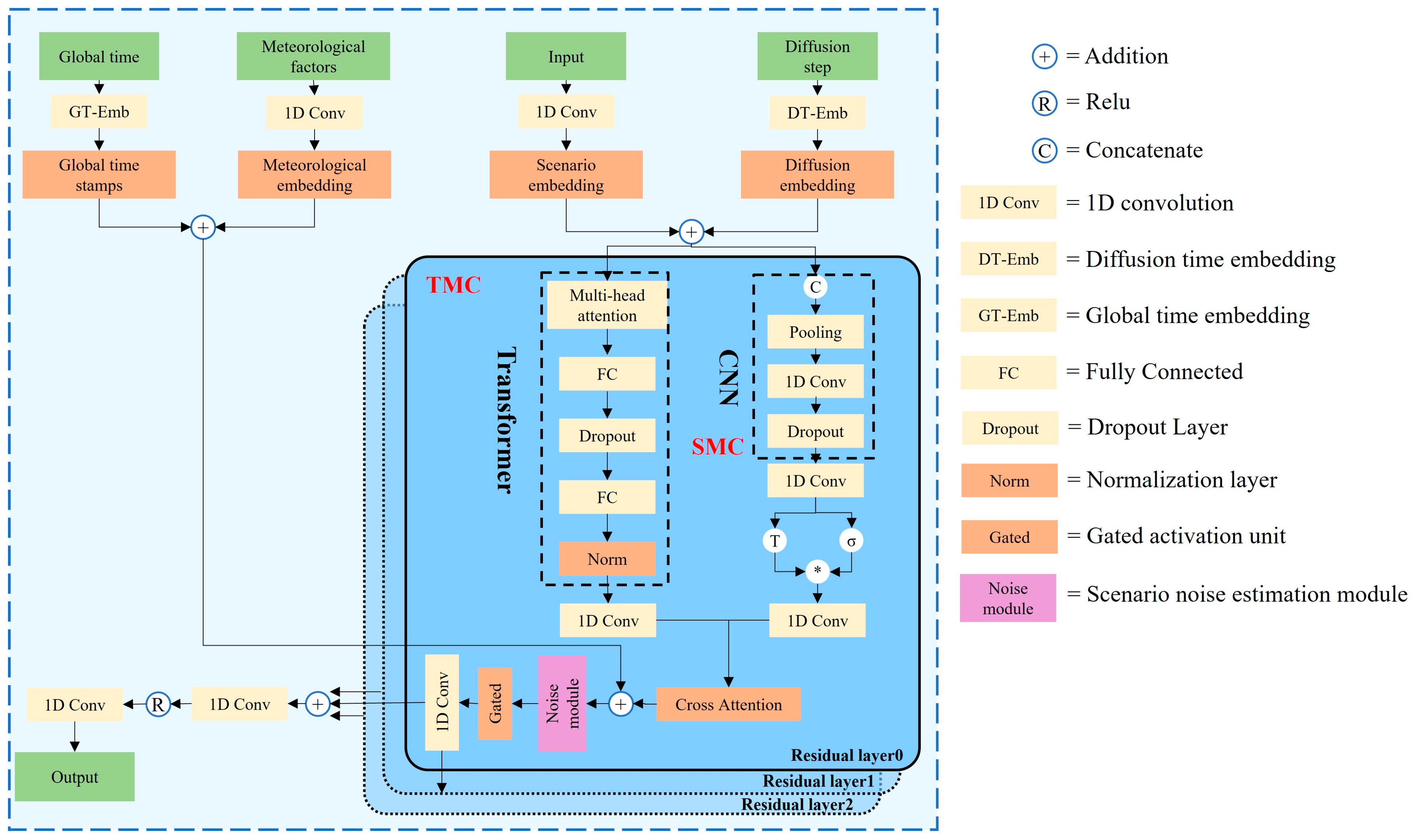
The randomness introduced by Gaussian noise leads to pattern instability in generated scenes, causing inconsistencies between noisy scenes and original scenes, especially when the diffusion stride $t$ approaches $T$. Consequently, adaptively learning weights from the hybrid of conditional information and source load scenes to obtain spatial-temporal correlation features become challenging [35]. To address these issues, this study proposes STF-CDM. The model’s primary innovation lies in designing the scene noise prediction network ϵθ, which comprises two modules: Temporal module component (TMC) and Spatial module component (SMC). These modules extract temporal and spatial features from the original information.

As shown in Figure 4, during pretraining, TMC and SMC focus on modeling the temporal and spatial correlations of the loading scenario. The collaborative design of TMC and SMC achieves deep integration through a cross-attention mechanism, jointly ensuring high fidelity in generated scenes. Specifically, TMC is built upon the Transformer architecture, with its core multi-head self-attention mechanism endowing the model with unparalleled capabilities for modeling long-range temporal dependencies. TMC can directly establish global dependencies between any two time points within a sequence, avoiding information decay or vanishing gradients caused by excessively long sequences. This enables the model to accurately learn and reproduce complex temporal characteristics in source-load data.

SMC efficiently captures local features and spatial dependencies within the regularized spatial dimension of the generated scene using a CNN foundation. This approach leverages the sequential or quasi-grid-like spatial arrangement of source-load variables, enabling the model to identify intrinsic patterns within local spatial configurations while enhancing computational efficiency and robustness.

The outputs from TMC and SMC are not simply concatenated but adaptively fused through a cross-attention mechanism. This mechanism uses the extracted temporal features (TMC output) as the Query, while the spatial features (SMC output) serve as both Key and Value. It dynamically calculates and integrates relevant information across temporal and spatial dimensions, generating high-quality scenes with consistent spatial-temporal coherence.

TMC is used to extract temporal features $F^{tem}$ by integrating two inputs: source observations $x_0$ and diffusion steps $t$. The diffusion steps $t$ are encoded as differences using 128-dimensional temporal embeddings as shown in Equation (36).

$$X=(Conv(x_0)+Fc(dif{f}_{emd}))$$

(36)

Then the queries ($Q_i^{tem}$), keys ($K_i^{tem}$) and values ($V_i^{tem}$) in the TMC are calculated as shown in Equation (37).

$$\left\{\begin{array}{l}{Q}_i^{tem}=X{W}_{q,i}^{tem}\\ K_i^{tem}=X{W}_{k,i}^{tem}\\ V_i^{tem}=X{W}_{\nu ,i}^{tem}\end{array}\right.$$

(37)

where $W_{q,i}^{tem}$, $W_{k,i}^{tem}$, $W_{\nu ,i}^{tem}$ are corresponding weighted matrices for $Q_i^{tem}$, $K_i^{tem}$, $V_i^{tem}$. The output $h_i^{tem}$ of the $i$-th attention head is computed as shown in Equation (38).

$$h_i^{tem}=softmax\left({\displaystyle \frac{Q_i^{tem}{\left(K_i^{tem}\right)}^T}{\sqrt{d_k^{tem}}}}\right)V_i^{tem}$$

(38)

where $softmax$ is a activation function, and $d_k^{tem}$ acts as a scaling factor to prevent gradient explosion. The multi-head representation is obtained by concatenating the representations produced by $y$ individual self-attention head which is shown in Equation (39).

$$MultiHea{d}^{tem}=Concat\left(h_1^{tem},h_2^{tem},\cdots ,h_y^{tem}\right)W_i^o$$

(39)

where y denotes the total amount of self-attention heads, Additionally, the normalization and dropout layers are intended to improve the stability of the TMC. Finally, Conv1d is further leveraged to extract the temporal features $F^{tem}$ which as shown in Equation (40).

$$F^{tem}=W^{tem}(MultiHea{d}^{pro})$$

(40)

where $W^{tem}$ is the parameter matrix and $MultiHea{d}^{pro}$ is the $MultiHea{d}^{tem}$ processed by the dropout and normalization layers.

Within SMC, this study employs a CNN to efficiently capture local features and spatial dependencies of generated scenes across regularized spatial dimensions. This design assumes that different source-load variables can be regarded as nodes arranged in an ordered sequence within the spatial dimension, where significant local spatial correlations exist between neighboring variables.

Specifically, the processed composite input $X\in R^{N\times d\times L}$ (where N is the batch size, d is the number of variables (treated as spatial dimensions), and L is the time step) is directly treated as a one-dimensional spatial signal with d channels and length L. This study employs one-dimensional convolutional layers to slide along the spatial dimension, capturing local patterns among neighboring variables.

The core propagation rule for a single one-dimensional convolution operation is shown in Equation (41).

$$H^{l+1}=\mathrm{Re}LU\left(Conv1D(H^l,W^{(l)},b^{(l)})\right)$$

(41)

where $H^l$ denotes the output features of layer l ($H^0$ = $X$), where $Conv1D$ represents a one-dimensional convolution operation. $W^{(l)}$ and $b^{(l)}$ are the learnable convolution kernel parameters and bias terms for this layer, respectively. The kernel size defines the receptive field, controlling the extent to which local spatial correlations are captured.

To integrate multi-level spatial features, this study aggregates outputs from different convolutional layers. Specifically, a two-layer CNN architecture is employed, with its outputs skip-connected to the original input before being fed into a final convolutional layer for information consolidation, as shown in Equation (42).

$$X_{CNN}=Conv1D\left(Concat\left(X,H^1,H^2\right)\right)$$

(42)

Apply a gated activation mechanism to enhance nonlinear expression capabilities and obtain the final spatial features of the SMC, as shown in Equation (43).

$$F^{spa}=tanh\{W^{f^{\ast }}\ast X_{GCN}\}\odot \sigma \{W^{g^{\ast }}\ast X_{GCN}\}$$

(43)

where $W^{f\ast }$, $W^{g\ast }$ are the learnable matrix parameters.

Simultaneously, the extracted temporal and spatial features are adaptively fused using a cross-attention mechanism. The acquisition of spatial-temporal features is illustrated in Equation (44).

$$F^{cstfm}=softmax\left({\displaystyle \frac{Q^{cstfm}{\left(K^{cstfm}\right)}^T}{\sqrt{d_k^{cstfm}}}}\right)V^{cstfm}$$

(44)

Attention weights are computed using the temporal feature $F^{{tem}^{\ast }}$ and the spatial feature $F^{{spa}^{\ast }}$. In practical applications, using the temporal feature $F^{{tem}^{\ast }}$ as the query and the spatial feature $F^{{spa}^{\ast }}$ as the key-value pair has yielded excellent performance which as shown in Equation (45).

$$Q^{cstfm}=F^{{tem}^{\ast }}{W}_q^{cstfm},K^{cstfm}=F^{{spa}^{\ast }}{W}_k^{cstfm},V^{cstfm}=F^{{spa}^{\ast }}{W}_{\nu }^{cstfm}$$

(45)

where $W_q^{cstfm}$, $W_k^{cstfm}$, $W_{\nu }^{cstfm}$ are learnable weight parameter matrices.

3.3. Evaluation Metrics

To further evaluate the superiority of the proposed CDM model, this study employs not only MAE and RMSE but also introduces two additional evaluation metrics—Frechet inception distance (FID) [36] and continuous ranked probability score (CRPS) [37]—to assess the model’s performance.

The FID is defined as shown in Equation (46).

$$FID\left(P_r,P_g\right)={\Vert u_r-u_g\Vert }_2^2+T_r\left(C_r+C_g-2{\left(C_r{C}_g\right)}^{1/2}\right)$$

(46)

CRPS is used to evaluate the fit between the estimated probability distribution of the generated scenario and the actual scenario. A smaller CRPS value indicates higher fidelity of the generated scenario. For a given load scenario x and its generated source load probability distribution $P$, CRPS measures the fit between $P$ and $x$ through the integral quantile loss ${\mathsf{\Lambda }}_{\alpha }$, as shown in Equations (47) and (48).

$$CRPS\left(P^{-1},x\right)={\int }_0^{1}2{\mathsf{\Lambda }}_{\alpha }\left(P^{-1}(\alpha ),x\right)d\alpha$$

(47)

$${\mathsf{\Lambda }}_{\alpha }\left(P^{-1}(\alpha ),x\right)=\left(\alpha -{\mathsf{\Pi }}_{x<P^{-1}(\alpha )}\right)\left(x-P^{-1}(\alpha )\right)$$

(48)

where α is the quantile levels; P⁻¹(α) is the α-quantile of P; Π is the indicator function.

4. Two-Stage DRO

This study employs the CDM model to generate scenarios and constructs an uncertainty set through downscaling to build a two-stage DRO model. The first stage of the two-stage distributed robust optimization model addresses the main problem, determining the energy trading plan with external parties prior to uncertainty occurrence. The second stage tackles the max-min problem: given the first-stage decision, it seeks a dispatch plan within the uncertainty set that accounts for the worst-case probability of renewable energy output scenarios. This plan is then fed back to the first stage to adjust the decision accordingly. Stages one and two iterate through alternating optimization until the first-stage decision satisfies all scenarios within the uncertainty set. The primary expression for the two-stage DRO is shown in Equation (49).

$$\left\{\begin{array}{l}\underset{x\in X}{\min }{a}^{\mathrm{T}}x+\underset{p_k\in \mathsf{\Omega }}{\max }\underset{y_k\in Y}{\min }{\displaystyle \sum _{k=1}^K}{p}_k{b}^{\mathrm{T}}{y}_k\\ Cx+Dz⩽d\\ Ex+F{y}_k⩽h,\forall k\in K\end{array}\right.$$

(49)

where $K$ denotes the total number of scenarios after clustering; $\mathsf{\Omega }$ denotes the confidence interval for the comprehensive norm; $C$, $D$, $E$, $F$, $d$, $h$ denote constant coefficient matrices.

The probability distribution of scenarios obtained through scenario clustering contains certain errors. To make the probability distribution more closely align with real data, the uncertainty confidence set presented in this section centers on the initial probability distribution and constrains the scenario probability distribution using a composite norm, thereby obtaining the worst-case probability distribution for each discrete scenario. The composite norm probability confidence interval, composed of the 1-norm and ∞-norm, is defined in Equation (50).

$$\left\{\begin{array}{l}\mathrm{Pr}\{{\displaystyle \sum _{k=1}^K}|p_k-p_{k0}|⩽{\theta }_1\}⩾1-2K{\mathrm{e}}^{-{\displaystyle \frac{2M{\theta }_1}{K}}}\\ \mathrm{Pr}\{\underset{1⩽k⩽K}{\max }|p_k-p_{k0}|⩽{\theta }_{\infty }\}⩾1-2K{\mathrm{e}}^{-2M{\theta }_{\infty }}\end{array}\right.$$

(50)

where $\mathrm{Pr}$ denotes the probability operator; $p_{k0}$ represents the number of generated samples; is the initial probability value for discrete scenario k; ${\theta }_1$ and ${\theta }_{\infty }$ denote the probability tolerance limits under the 1-norm and ∞-norm constraints, respectively.

To solve this inequality, transform it as shown in Equation (51).

$$\left\{\begin{array}{l}{\theta }_1={\displaystyle \frac{K}{2M}}\ln {\displaystyle \frac{2K}{1-{\alpha }_1}}\\ {\theta }_{\infty }={\displaystyle \frac{1}{2M}}\ln {\displaystyle \frac{2K}{1-{\alpha }_{\infty }}}\end{array}\right.$$

(51)

Thus, the confidence interval for the composite norm is shown in Equation (52).

$$\mathsf{\Omega }=\left\{\begin{array}{l}{p}_k|p_k⩾0,k=1,\cdots ,K;{\displaystyle \sum _{k=1}^K}{p}_k=1;\hfill \\ {\displaystyle \sum _{k=1}^K}|p_k-p_{k0}|⩽{\theta }_1;\underset{1⩽k⩽K}{\max }|p_k-p_{k0}|⩽{\theta }_{\infty }\hfill \end{array}\right.$$

(52)

5. MIES Game Theory Model and Solutions

5.1. Asymmetric Revenue Allocation

Each IES contributes varying amounts of energy to the alliance, resulting in differing bargaining power. IES revenues are allocated based on this bargaining power. The proposed asymmetric revenue allocation is shown in Equation (53).

$$\left\{\begin{array}{c}\max {\displaystyle \underset{i=1}{\overset{N}{\mathsf{\Pi }}}}{(C_i^0-C_i^1+C_i^{\mathrm{P}2\mathrm{P}})}^{S_i}\\ \mathrm{s}.\mathrm{t}.C_i^{0^{\ast }}-C_i^{1^{\ast }}+C_i^{\mathrm{P}2\mathrm{P}}⩾0\end{array}\right.$$

(53)

where $C_i^0$ and $C_i^{0^{\ast }}$ denote the pre-cooperation cost and optimal cost for IES, respectively; $C_i^1$ and $C_i^{1^{\ast }}$ denote the cooperation cost without payment consideration and optimal cooperation cost for IES.

5.2. Model Subproblem Construction

The Nash bargaining model can be equivalently formulated as solving the subproblems of maximizing cooperative benefits and energy payments. The expressions for subproblem 1 and subproblem 2 are shown in Equations (54) and (55).

$$\left\{\begin{array}{l}\min C_i^1=\min {\displaystyle \sum _{i=1}^N}{\mathit{a}}^{\mathrm{T}}x+\underset{p_k\in \mathsf{\Omega }}{\max }\underset{y_k\in Y}{\min }{\displaystyle \sum _{i=1}^N}{\displaystyle \sum _{k=1}^K}{p}_k{\mathit{b}}^{\mathrm{T}}{y}_k\hfill \\ \mathrm{s}.\mathrm{t}.(49)\hfill \end{array}\right.$$

(54)

$$\begin{array}{c}\left\{\begin{array}{ll}\max {\displaystyle \underset{i=1}{\overset{N}{\mathsf{\Pi }}}}{(C_i^0-C_i^{1^{\ast }}+C_i^{\mathrm{P}2\mathrm{P}})}^{S_i}\hfill & \hfill \\ \mathrm{s}.\mathrm{t}.C_i^0-C_i^{1^{\ast }}+C_i^{\mathrm{P}2\mathrm{P}}⩾0\hfill & \hfill \\ C_i^{\mathrm{P}2\mathrm{P}}=p_{i-j}^{\mathrm{P}2\mathrm{P},\mathrm{e}}{P}_{i-j,\mathrm{e},t}^{\mathrm{P}2\mathrm{P}}+p_{i-j}^{\mathrm{P}2\mathrm{P},\mathrm{h}}{P}_{i-j,\mathrm{h},t}^{\mathrm{P}2\mathrm{P}}\hfill & \hfill \\ p_{i-j,\min }^{\mathrm{P}2\mathrm{P},\mathrm{e}}⩽p_{i-j}^{\mathrm{P}2\mathrm{P},\mathrm{e}}⩽p_{i-j,\max }^{\mathrm{P}2\mathrm{P},\mathrm{e}}\hfill & \hfill \\ p_{i-j,\min }^{\mathrm{P}2\mathrm{P},\mathrm{h}}⩽p_{i-j}^{\mathrm{P}2\mathrm{P},\mathrm{h}}⩽p_{i-j,\max }^{\mathrm{P}2\mathrm{P},\mathrm{h}}\hfill & \hfill \end{array}\right.\end{array}$$

(55)

where $C_i^{1^{\ast }}$ denotes the optimal solution obtained for subproblem 1; $p_{i-j}^{\mathrm{P}2\mathrm{P},\mathrm{e}}$, $p_{i-j}^{\mathrm{P}2\mathrm{P},\mathrm{h}}$ denotes the interaction electricity price and the interactive heat price; $p_{i-j,\min }^{\mathrm{P}2\mathrm{P},\mathrm{e}}$, $p_{i-j,\max }^{\mathrm{P}2\mathrm{P},\mathrm{e}}$, $p_{i-j,\min }^{\mathrm{P}2\mathrm{P},\mathrm{h}}$, $p_{i-j,\max }^{\mathrm{P}2\mathrm{P},\mathrm{h}}$ represent its upper and lower bounds.

Bargaining power is a key factor determining revenue distribution. Therefore, nonlinear energy mapping is employed to quantify the bargaining power of each entity. This study quantifies the electrical and thermal energy contributions of each IES to establish a reasonable energy transaction price, thereby achieving equitable distribution. The specific expression is shown in Equations (56)–(58).

$$S_i=S_i^{\mathrm{a}}/\sum _{i=1}^N{S}_i^{\mathrm{a}}$$

(56)

$$\left\{\begin{array}{l}{S}_i^{\mathrm{a}}={\mu }_{\mathrm{e}}{S}_{i,\mathrm{e}}+{\mu }_{\mathrm{h}}{S}_{i,\mathrm{h}}\hfill \\ S_{i,\mathrm{e}}={\mathrm{e}}^{E_i^{\mathrm{supply}}/E_{\max }^{\mathrm{supply}}}-{\mathrm{e}}^{-(E_i^{\mathrm{receive}}/E_{\max }^{\mathrm{receive}})}\hfill \\ S_{i,\mathrm{h}}={\mathrm{e}}^{H_i^{\mathrm{supply}}/H_{\max }^{\mathrm{supply}}}-{\mathrm{e}}^{-(H_i^{\mathrm{receive}}/H_{\max }^{\mathrm{receive}})}\hfill \end{array}\right.$$

(57)

$$\left\{\begin{array}{c}{E}_i^{\mathrm{supply}}={\displaystyle \sum _{t=1}^T}\max (P_{i-j,\mathrm{e},t}^{\mathrm{P}2\mathrm{P}},0)\\ E_i^{\mathrm{receive}}=-{\displaystyle \sum _{t=1}^T}\max (P_{i-j,\mathrm{e},t}^{\mathrm{P}2\mathrm{P}},0)\\ H_i^{\mathrm{supply}}={\displaystyle \sum _{t=1}^T}\max (P_{i-j,\mathrm{h},t}^{\mathrm{P}2\mathrm{P}},0)\\ H_i^{\mathrm{receive}}=-{\displaystyle \sum _{t=1}^T}\max (P_{i-j,\mathrm{h},t}^{\mathrm{P}2\mathrm{P}},0)\end{array}\right.$$

(58)

where $S_i$ represents the normalized quantitative value of each IES’s bargaining power $S_i^{\mathrm{a}}$; $S_{i,\mathrm{e}}$ and $S_{i,\mathrm{h}}$ denote the quantitative values of each IES’s bargaining power for electrical energy and thermal energy, respectively; ${\mu }_{\mathrm{e}}$ and ${\mu }_{\mathrm{h}}$ denote the contribution ratios of electrical energy and thermal energy to bargaining, respectively; $E_i^{\mathrm{supply}}$ and $H_i^{\mathrm{supply}}$ denote the total electrical energy and thermal energy supplied by the microgrid when participating in cooperation. $E_i^{\mathrm{receive}}$ and $H_i^{\mathrm{receive}}$ represent the total electrical and thermal energy received by the microgrid during cooperation.

5.3. Model Solution Method

The objective function of Subproblem 1 is decomposable. Based on the ADMM algorithm principle, for IES i, construct the augmented Lagrangian function as shown in Equation (59).

$$\left\{\begin{array}{l}{L}_i(P_{i-j,\mathrm{e}/\mathrm{h},t}^{\mathrm{P}2\mathrm{P}},P_{j-i,\mathrm{e}/\mathrm{h},t}^{\mathrm{P}2\mathrm{P}},{\lambda }_{i-j,t}^{\mathrm{e}/\mathrm{h}},{\rho }_{i-j,t}^{\mathrm{e}/\mathrm{h}})=\underset{x,z}{\min }{\mathit{a}}^{\mathrm{T}}x+{\displaystyle \sum _{i\in N}}{\lambda }_{i-j,t}^{\mathrm{e}/\mathrm{h}}(P_{i-j,\mathrm{e}/\mathrm{h},t}^{\mathrm{P}2\mathrm{P}}+P_{j-i,\mathrm{e}/\mathrm{h},t}^{\mathrm{P}2\mathrm{P}})+\\ {\displaystyle \sum _{i\in N}}{\displaystyle \frac{{\rho }_{i-j,t}^{\mathrm{e}/\mathrm{h}}}{2}}\parallel P_{i-j,\mathrm{e}/\mathrm{h},t}^{\mathrm{P}2\mathrm{P}},P_{j-i,\mathrm{e}/\mathrm{h},t}^{\mathrm{P}2\mathrm{P}}{\parallel }_2^2+\underset{p_k\in \mathsf{\Omega }}{\max }\underset{y_k\in Y}{\min }{\displaystyle \sum _{k\in K}}{p}_w{\mathit{b}}^{\mathrm{T}}{y}_k\\ \mathrm{s}.\mathrm{t}.(49)\end{array}\right.$$

(59)

For two-stage robust optimization problems, since each scenario problem is independent, a parallel solution approach can be adopted. First, solve the k min problems separately, then solve the max problem. This avoids the inefficiency caused by deriving the dual form and introducing 0–1 variables. After obtaining the worst-case scenario probability, solve the main and subproblems iteratively using the C&CG algorithm. Atomic Problem 1 is decomposed into a main problem and a subproblem. Through iterative solutions of the main and subproblems, the optimal solution of the model is obtained.

The expressions for the main problem and subproblems are shown in Equations (60) and (61).

$$\left\{\begin{array}{l}\underset{x,z}{\min }{\mathit{a}}^{\mathrm{T}}x+{\displaystyle \sum _{i\in N}}{\lambda }_{i-j,t}^{\mathrm{e}/\mathrm{h}}(P_{i-j,\mathrm{e}/\mathrm{h},t}^{\mathrm{P}2\mathrm{P}}+P_{j-i,\mathrm{e}/\mathrm{h},t}^{\mathrm{P}2\mathrm{P}})+{\displaystyle \sum _{i\in N}}{\displaystyle \frac{{\rho }_{i-j,t}^{\mathrm{e}/\mathrm{h}}}{2}}\parallel P_{i-j,\mathrm{e}/\mathrm{h},t}^{\mathrm{P}2\mathrm{P}}+P_{j-i,\mathrm{e}/\mathrm{h},t}^{\mathrm{P}2\mathrm{P}}{\parallel }_2^2+\eta \\ \mathrm{s}.\mathrm{t}.\mathit{C}x+\mathit{D}z⩽\mathit{d}\\ \mathit{E}x+\mathit{F}{y}_k⩽\mathit{h},\forall k\in K\\ \eta ⩾{\displaystyle \sum _{y_k\in Y}}{p}_{k^{\ast }}{\mathit{b}}^{\mathrm{T}}{y}_k\end{array}\right.$$

(60)

$$\left\{\begin{array}{l}{\displaystyle \underset{p_k\in \mathsf{\Omega }}{\max }}{\displaystyle \underset{y_k\in Y}{\min }}{\displaystyle \sum _{k=1}^K}{p}_k{\mathit{b}}^{\mathrm{T}}{y}_k\hfill \\ \mathrm{s}.\mathrm{t}.\mathit{E}{x}^{\ast }+\mathit{F}{y}_k⩽\mathit{h},\forall k\in K\hfill \end{array}\right.$$

(61)

Since the inner decision variables are independent across different scenarios, the inner layer of the subproblem can be decomposed into K independent linear programming problems and solved simultaneously using parallel computing methods. Therefore, subproblem (61) can be equivalently expressed as shown as Equation (62).

$$\left\{\begin{array}{l}{\displaystyle \underset{p_k\in \mathsf{\Omega }}{\max }}{\displaystyle \sum _{k=1}^K}{p}_k{\mathit{b}}^{\mathrm{T}}{y}_k^{\ast }\\ {y_k}^{\ast }=\arg {\displaystyle \underset{y_k^{\ast }Y}{\min }}{\mathit{b}}^{\mathrm{T}}{y}_k^{\ast }\\ \mathrm{s}.\mathrm{t}.\mathit{E}{x}^{\ast }+\mathit{F}{y}_k⩽\mathit{h},\forall k\in K\end{array}\right.$$

(62)

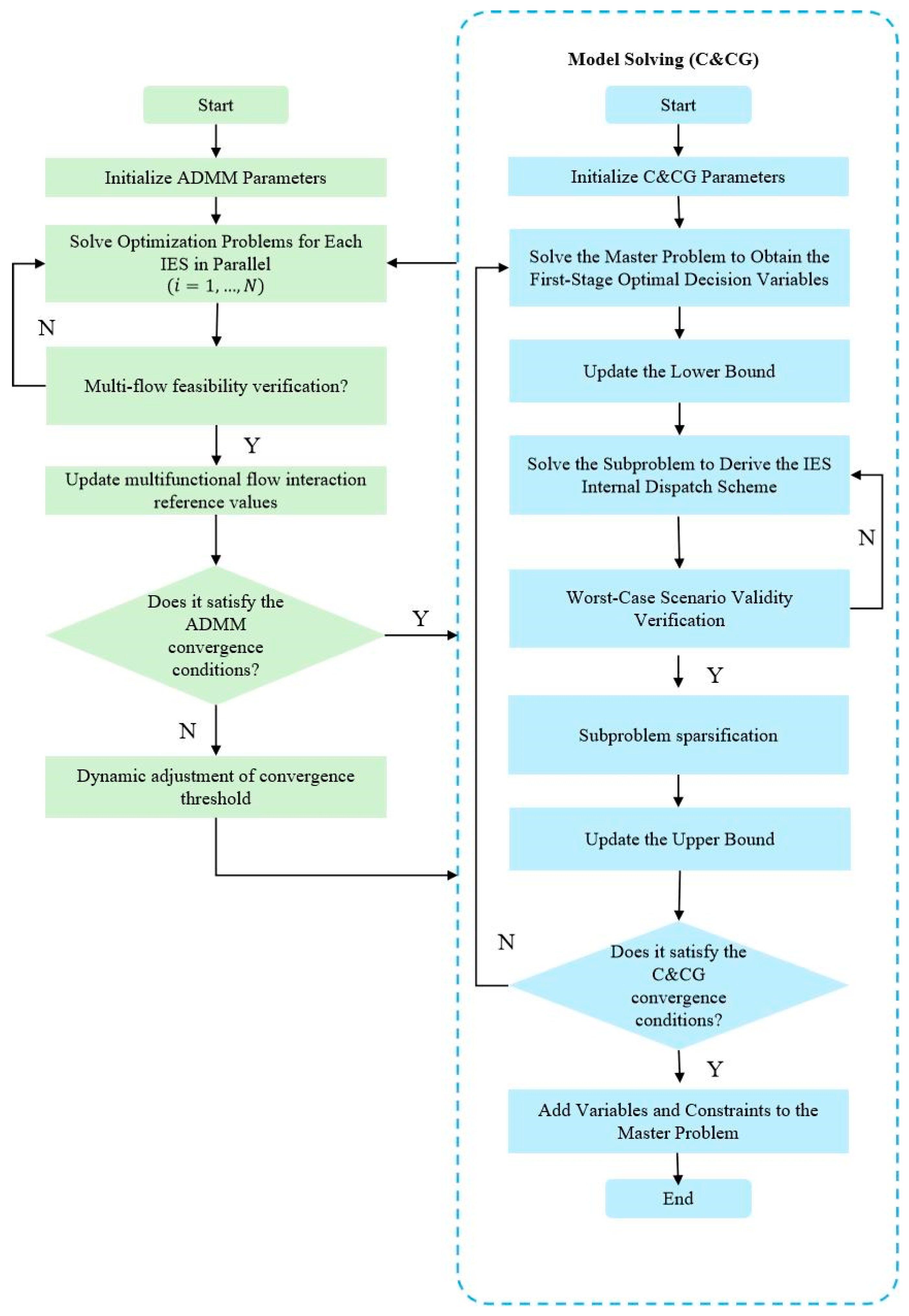
The process of solving Subproblem 1 using the ADMM-C&CG algorithm based on coupled parallel computation is illustrated in Figure 5.

The pseudocode for implementing the MIES optimization scheduling process is shown in Algorithm 1.

Algorithm 1 Distributed ADMM-C&CG for MIES Scheduling

Require: Number of IES $N$, convergence tolerance $\epsilon$, penalty factor $\rho$, renewable generation scenarios

Ensure: Optimal MIES scheduling results

1: Initialize ADMM iteration index $m\leftarrow 1$

2: Initialize inter-IES power flows $P^{\mathrm{P}2\mathrm{P}}$, Lagrange multipliers $\lambda$

3: Generate initial renewable scenarios and probabilities via STF-CDM and K-means

4: while not converged do

5:        for $i=1$ to $N$ (in parallel) do

6:                Solve internal optimization via C&CG

7:        end for

8:        for each IES pair $(i,j)$ do

9:                Update power exchange variables:

${P_{i\to j}^{\mathrm{P}2\mathrm{P},m+1}=\mathit{argmin}}_{P_{i\to j}^{\mathrm{P}2\mathrm{P}}}{\mathcal{L}}_{\mathcal{i}}\left(P_{i\to j}^{\mathrm{P}2\mathrm{P}},P_{j\to i}^{\mathrm{P}2\mathrm{P}},{\lambda }_{i\to j}^m\right)$ ${P_{j\to i}^{\mathrm{P}2\mathrm{P},m+1}=\mathit{argmin}}_{P_{j\to i}^{\mathrm{P}2\mathrm{P}}}{\mathcal{L}}_{\mathcal{j}}\left(P_{i\to j}^{\mathrm{P}2\mathrm{P}},P_{j\to i}^{\mathrm{P}2\mathrm{P}},{\mathsf{\lambda }}_{j\to i}^m\right)$

10:                Update Lagrange multiplier ${\lambda }_{i\to j}^m$${\mathsf{\lambda }}_{j\to i}^m$

11:        end for

12:        If  ma$x\left\{{\sum }_{t=1}^T|\left(P_{i\to j,t}^{\mathrm{P}2\mathrm{P}}+P_{j\to i,t}^{\mathrm{P}2\mathrm{P}}\right){|}_2^2\right\}\le \mathsf{\epsilon }$ then

13:                break

14:                end if

15: Update penalty factor $\rho$

$m\leftarrow m+1$

16: end while

17: Output optimal MIES scheduling results

6. Results and Discussion

6.1. Data

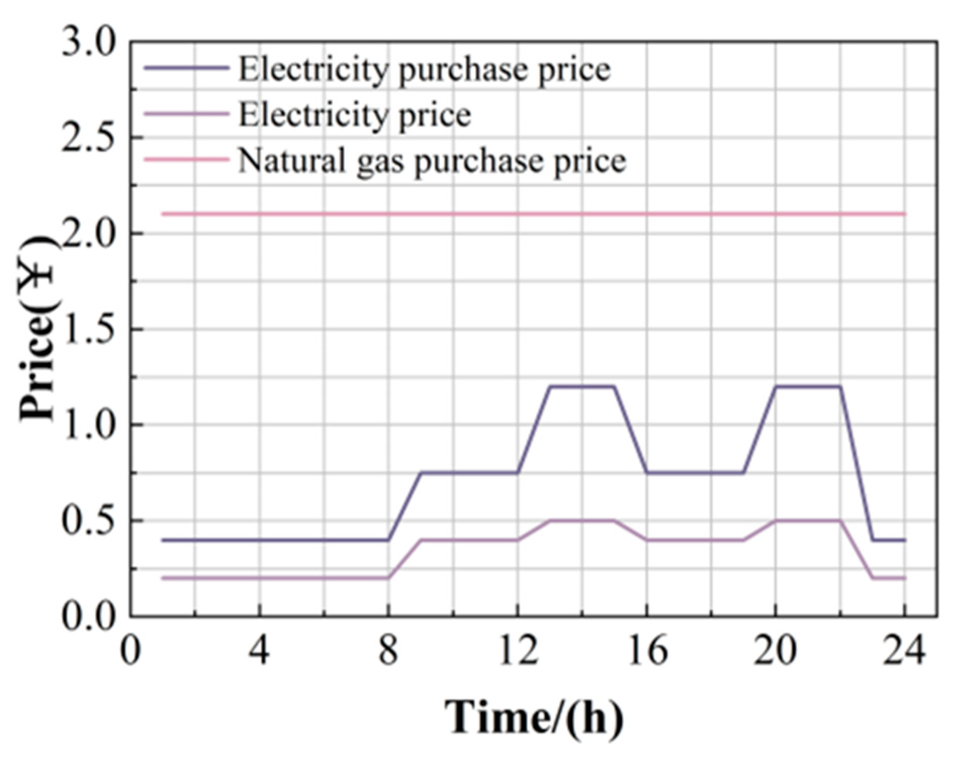
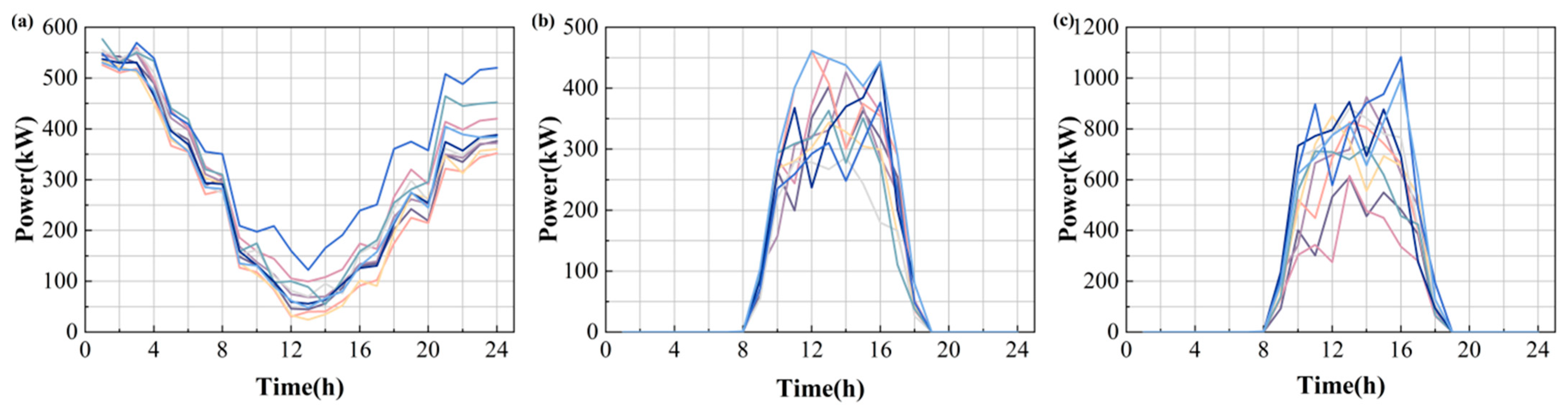
The raw data for renewable energy sources and energy prices are shown in Figure 6 and Figure 7.

Table 2. The maximum capacities of IES1, IES2, and IES3.

Parameters	IES 1	IES 2	IES 3
Photovoltaic capacity (kW)	0	400	900
Wind power capacity (kW)	600	0	0

shows the maximum capacities of IES1, IES2, and IES3, where IES1 is configured with wind power units, while IES2 and IES3 are equipped with photovoltaic power units.

Table 3. Simulation parameters.

Parameters	Value	Parameters	Value
${\eta }_{\mathrm{GT},\mathrm{e}}$	0.36	$P_{i,\mathrm{h},\max }^{\mathrm{HP}}$	800
${\eta }_{\mathrm{GT},\mathrm{h}}$	0.45	${\alpha }_{i,e}^{\max }$	0.9
$H_{\mathrm{GHV}}$	9.5	$P_{i,\mathfrak{c},\max }^{AC}$	1500
$P_{i,\mathrm{e},\max }^{\mathrm{GT}}$	1800	${\alpha }_{i,e}^{\min }$	0.1
${\eta }_{\mathrm{HP}}$	2.2	${\eta }_{\mathrm{AC}}$	1.2
${\delta }_{\mathrm{h}}$	0.05	${\alpha }_{i,h}^{\max }$	0.9
${\eta }_{\mathrm{e}}^{\mathrm{ch}}$	0.98	$P_{i,\mathfrak{c},\max }^{\mathrm{EC}}$	1000
${\eta }_{\mathrm{h}}^{\mathrm{ch}}$	0.95	${\alpha }_{i,h}^{\min }$	0.1
${\eta }_{\mathrm{e}}^{\mathrm{dis}}$	0.99	${\eta }_{\mathrm{EC}}$	4
${\eta }_{\mathrm{h}}^{\mathrm{dis}}$	0.95	$S_{\mathrm{h},\mathrm{rent}}^{\max }$	500
${\eta }_{\mathrm{P}2\mathrm{G}}$	0.55	$P_{i,\mathrm{e},\max }^{\mathrm{CCS}}$	200
$S_{\mathrm{e},\mathrm{rent}}^{\max }$	500	${\mu }_{\mathrm{e}}$	0.5
${\eta }_{\mathrm{CC}}$	1.06	${\mu }_{\mathrm{h}}$	0.5
$P_{\mathrm{e},\mathrm{rent}}^{\max }$	250	$P_{\mathrm{h},\mathrm{rent}}^{\max }$	250
${\eta }_{\mathrm{CCS}}$	0.5	$P_{i,\mathrm{e},\max }^{\mathrm{P}2\mathrm{G}}$	300

shows experimental parameters required for the simulation experiment. Renewable energy data and energy price data are derived from actual measurements of a multi-energy integrated system in Changchun. Experimental parameters are partially sourced from Ref. [25].

6.2. STF-CDM Model Experimental Results

This study employed the STF-CDM model to generate renewable energy scenarios for various IESs and utilized K-means clustering for scenario reduction, yielding representative renewable energy scenarios for each IES as shown in Figure 8. As shown in the figure, the generated scenarios fully cover the upper and lower fluctuation boundaries of the original scenarios. While ensuring accuracy, they achieve satisfactory results within a 95% confidence interval. The ideal scenario set can reproduce actual load trends and exhibits sufficient diversity in local random fluctuations to cover the range of possible scenarios. Simultaneously, the generated scenario set ensures the safety and robustness of subsequent DRO.

To comprehensively validate the effectiveness of the proposed method, this study conducted comparative experiments between the STF-CDM model and current mainstream scene generation methods. The comparison models include Monte Carlo simulation (MC) [38], Latin Hypercube Sampling (LHS) [39], GAN [40], WGAN-GP [41], and diffusion models. Among these, The STF-CDM model training employs the Adam optimizer with a learning rate of 0.001, a batch size of 64, and 200 training epochs. The TMC module utilizes a 4-layer Transformer architecture with 4 attention heads per layer; the SMC module employs a 3-layer 1D CNN with convolutional kernel sizes of 3, 5, and 7. The MC method employed 5000 samples; both GAN and WGAN-GP utilized a 4-layer MLP network with a learning rate of 0.0002, Adam optimizer, batch size of 64, and training for 10,000 epochs. All models were trained on identical GTX 5060 GPU hardware. To ensure fair comparison, all models underwent parameter tuning. Evaluation metrics encompass multiple statistical measures, including MAE, RMSE, CRPS, and FID. Simulation results are presented in

Table 4. Evaluation metrics of experiments.

Model	MAE	RMSE	CRPS	FID
MC	20.45	40.23	0.75	1150.82
LHS	18.33	36.87	0.70	1020.45
GAN	16.78	34.20	0.65	900.20
WGAN-GP	15.12	32.90	0.60	750.45
Diffusion model	13.65	28.50	0.52	620.89
STF-CDM	7.98	19.60	0.28	255.83

, with the best performing results highlighted in bold.

In comparative results, shown in Table 3, STF-CDM demonstrated outstanding performance during testing. Compared to the next-best model, STF-CDM achieved significant improvements. MAE decreased by 34.72%, RMSE by 21.61%, CRPS by 32.35%, and FID by 47.00%. The comparison results clearly indicate that STF-CDM’s advantage stems from its dedicated scene noise prediction network architecture—effectively capturing complex spatiotemporal correlations between scenes via TMC, while utilizing SMC to adaptively learn conditional information and weight distribution between scenes. Furthermore, the model’s gradual integration of generative mechanisms and conditional information during diffusion significantly enhances its ability to represent temporal dynamics in generated scenes, ultimately achieving an optimal balance between generation quality and diversity.

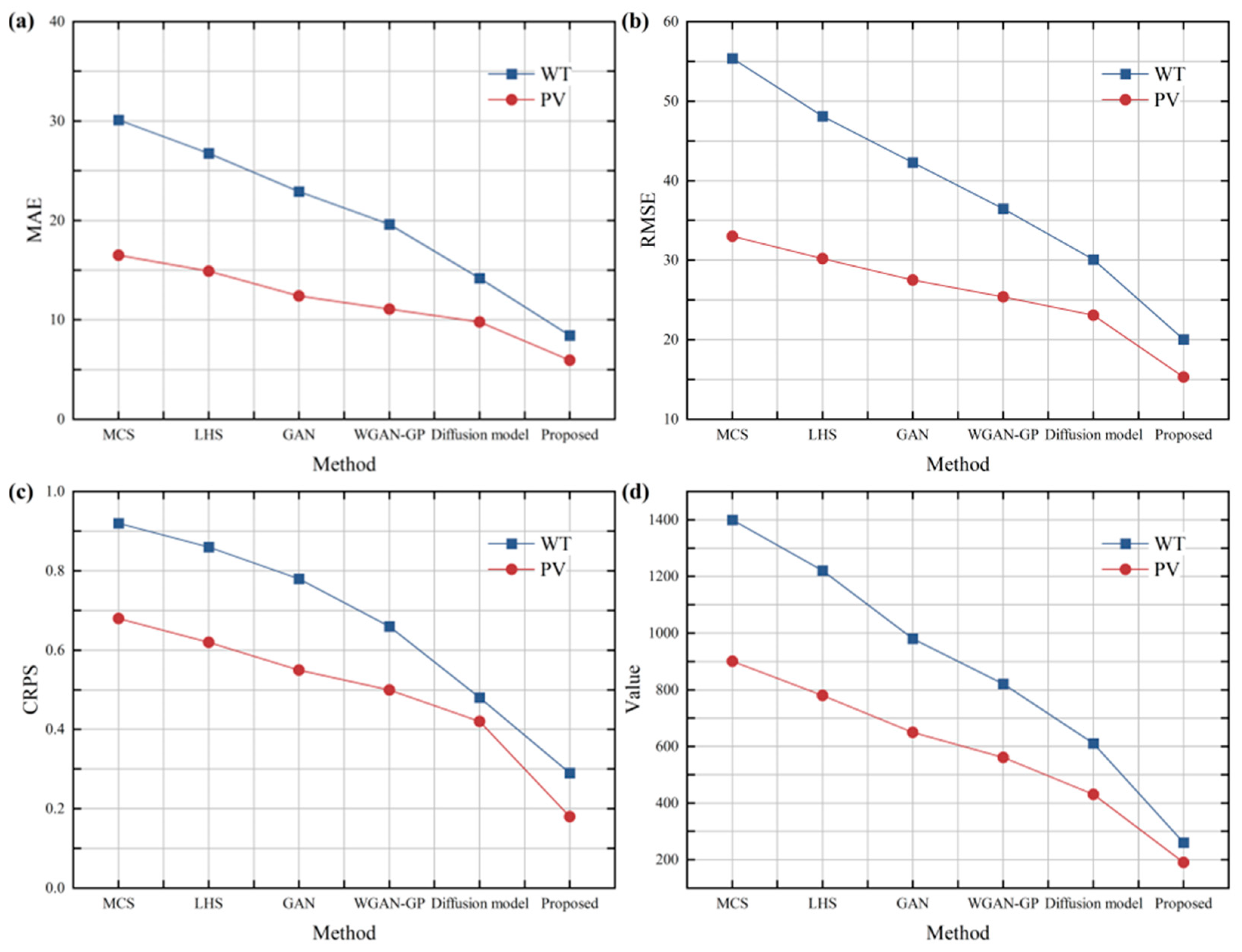
In addition to testing the overall performance metrics of the model, this study also conducted empirical data tests on wind power and photovoltaic data from IES 1 and IES 2. The results for each metric are shown in Figure 9. As illustrated in Figure 9, the STF-CDM model continues to demonstrate optimal performance, further validating its superiority in renewable energy scenario generation. This lays a crucial foundation for subsequent construction of robust optimization uncertainty sets.

6.3. ADMM-C&CG Optimization Results Analysis

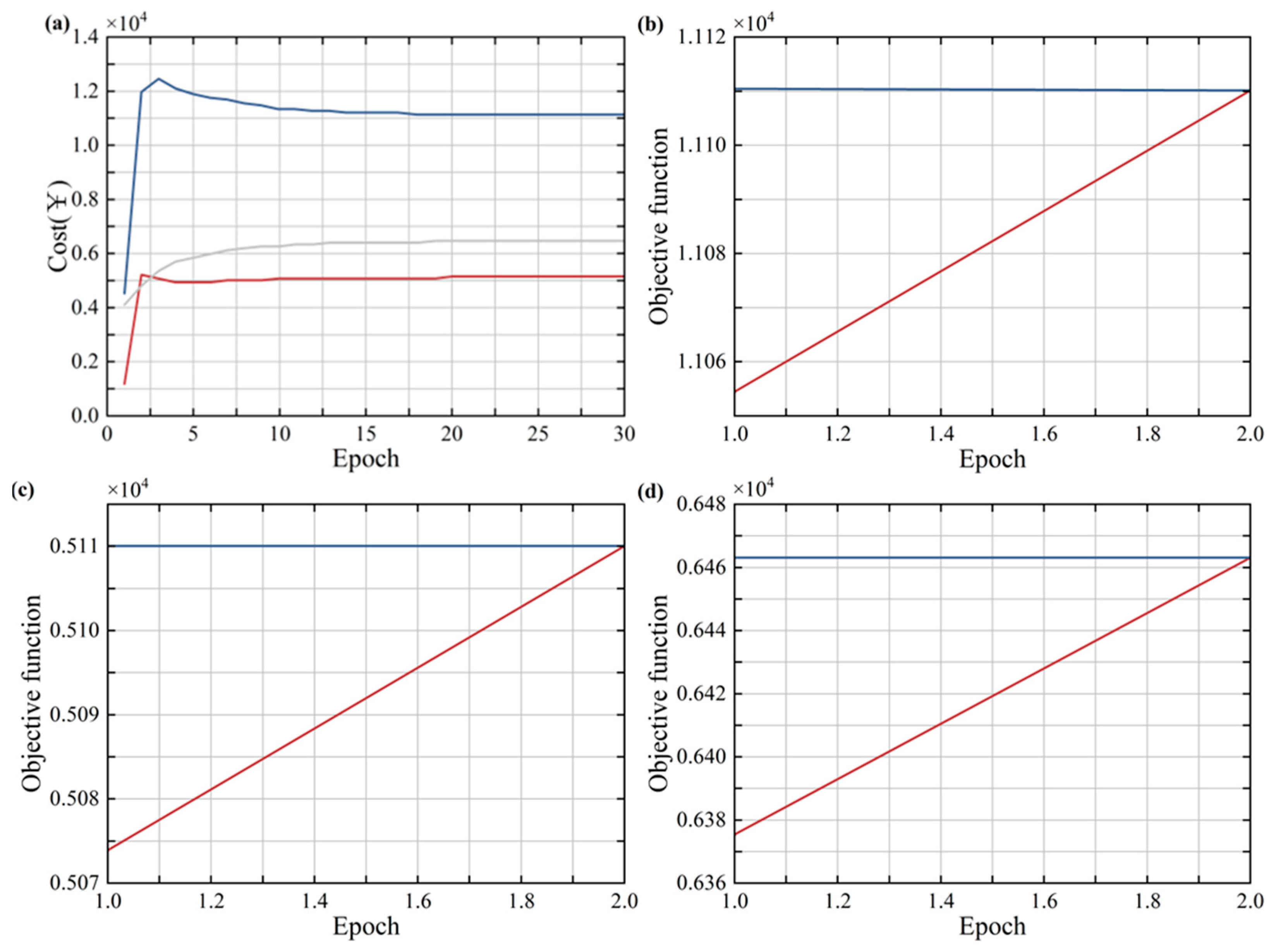
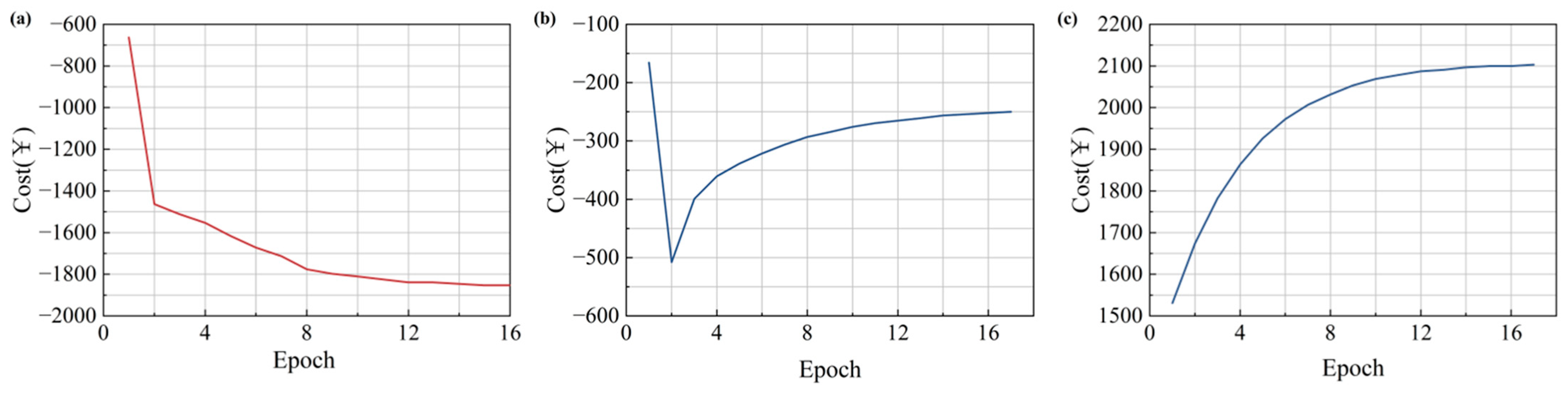
Figure 10 illustrates the convergence characteristics of the proposed parallel ADMM-C&CG algorithm when solving Subproblem 1, while Figure 11 shows the convergence trajectory of the ADMM’s computational cost when addressing Subproblem 2.

The results indicate that the ADMM algorithm converged after 34 iterations in Subproblem 1, taking 313 s. Subproblem 2 converged in just 17 iterations and 12 s. These findings confirm that the ADMM not only offers high computational efficiency and stable convergence for solving collaborative optimization problems but also effectively safeguards the privacy of data from all participating entities. On the other hand, the parallelizable C&CG algorithm demonstrated outstanding convergence speed—all IES subsystem models converged within 2 iterations. During optimization, the gap between upper and lower bounds progressively narrowed until meeting the preset tolerance range, indicating the C&CG algorithm’s excellent solution capability when handling complex internal IES models.

6.4. Optimization Results Analysis

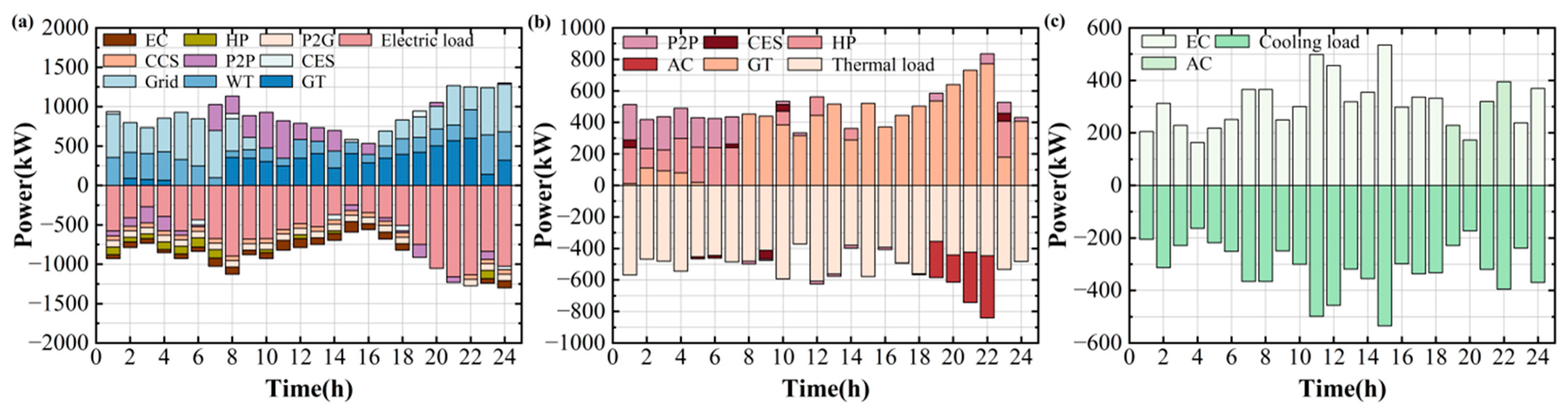
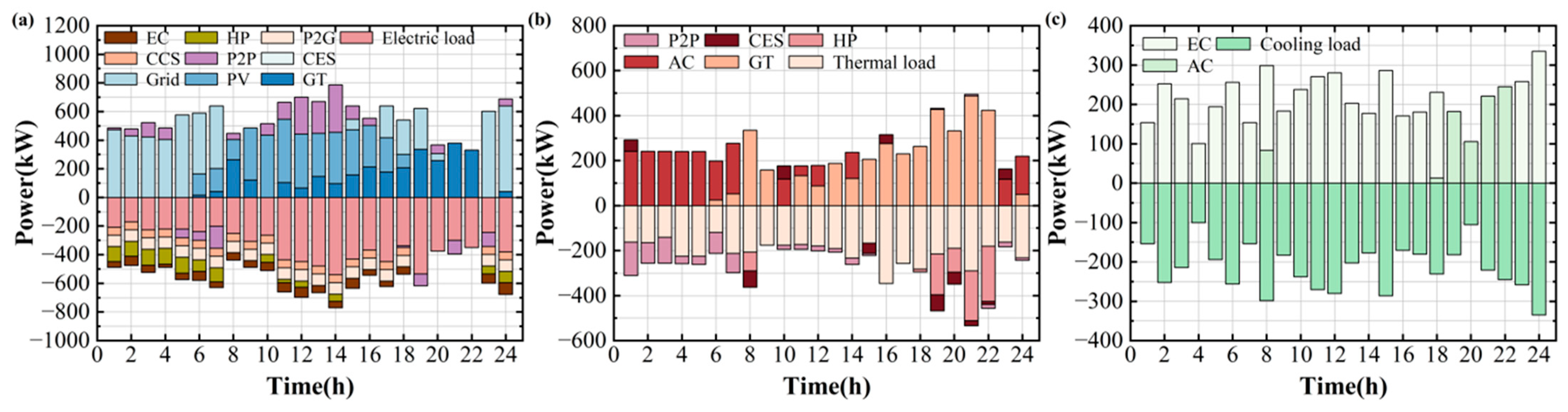
After each IES participates in electricity-to-heat peer-to-peer transactions, their respective optimized scheduling results are shown in Figure 12, Figure 13 and Figure 14. IES 1, benefiting from abundant wind resources, operates during local off-peak periods from 00:00 to 06:00 and 13:00 to 16:00. Excess wind power is stored via cloud energy storage, consumed through EC, P2G-CCS, and HP systems, and surplus electricity is sold to the external grid and other IES. During peak consumption periods from 07:00 to 12:00 and 16:00 to 23:00, after absorbing all wind power output, IES 1 meets load demand by increasing GT unit output, discharging CES systems, and purchasing electricity from other IES and the upper-level grid, thereby reducing the park’s total energy costs. As shown in Figure 12b, regarding thermal power optimization, during 00:00–07:00, IES 1 maintains thermal balance through HP output, GT output, CES heat charging, and P2P heat trading. During 19:00–22:00, excess thermal output from the GT unit is absorbed by heat consumption from the AC unit and heat release from CES, alleviating pressure on the EC. The analysis for cooling power follows the same principle.

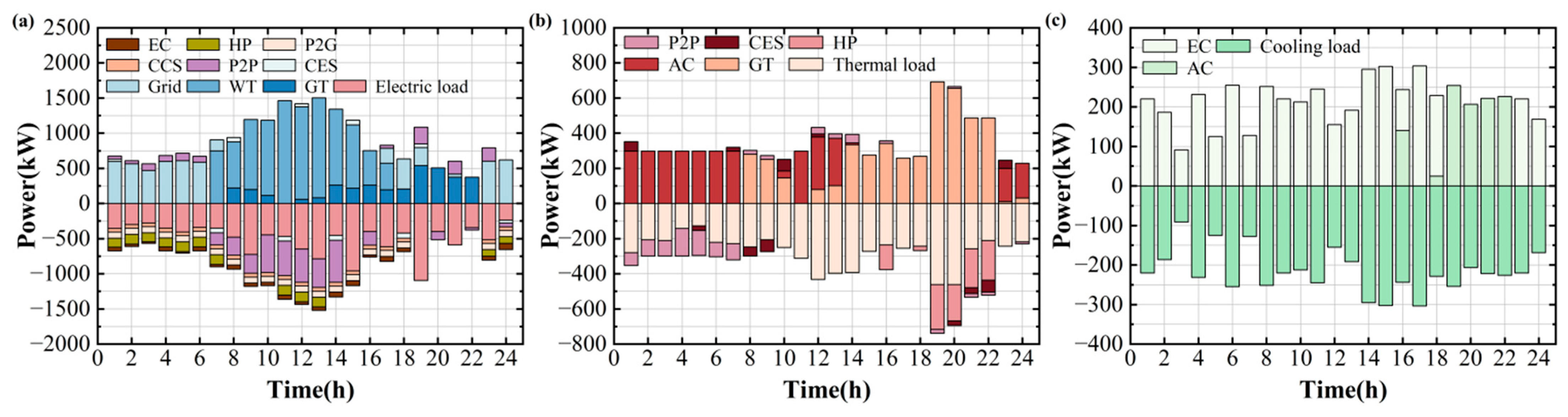
Based on the optimized scheduling results of IES 2 shown in Figure 13, this IES demonstrates significant complementarity with IES 1, which primarily relies on wind power. In terms of electricity, during the well-lit period from 07:00 to 17:00, IES 2 generates substantial surplus power from photovoltaic generation. This surplus not only meets local electricity demand but is also sold to IES 1 during its peak consumption hours via P2P transactions. Simultaneously, part of the electricity is stored in CES or utilized for energy conversion through HP and P2G systems. During nighttime and non-sunlit periods, IES 2 meets demand by purchasing electricity from the grid, utilizing CES, and acquiring wind power from IES 1. GT systems supplement demand with limited activation during evening peak loads. For thermal balance, HP primarily handles daytime heating using low-cost PV power while storing excess heat in CES. Nighttime demand is met by releasing CES thermal storage and GT waste heat, with P2P heat trading further optimizing cross-system thermal allocation. Cooling power scheduling follows a similar logic, primarily relying on EC operation during PV generation peaks to achieve spatiotemporal energy transfer.

As IES 3 shown in Figure 14, its scheduling mode is like IES 2 but exhibits subtle differences influenced by local load characteristics. As another PV system, IES 3 similarly prioritizes supporting IES 1 with surplus PV generation via the P2P grid during daytime hours while utilizing CES for energy storage. Unlike IES 2, IES 3’s thermal load curve may be flatter, enabling it to allocate more power during midday PV peak periods to drive AC units for cooling load satisfaction and storage via HP heating. During nighttime, IES 3 relies on CES discharge, purchased electricity (especially from IES 1), and flexible GT regulations to maintain power balance. Its thermal supply is dominated by HP during daytime, combined with CES for peak shaving and valley filling. During evening thermal load peaks, GT’s combined heat and power output increases, coordinating with CES to ensure supply, while P2P thermal transactions enhance inter-system redundancy and reliability. The coupled scheduling of thermal, electrical, and cooling energy fully demonstrates the economic efficiency and flexibility of photovoltaic-based IES supported by P2P transactions and CES.

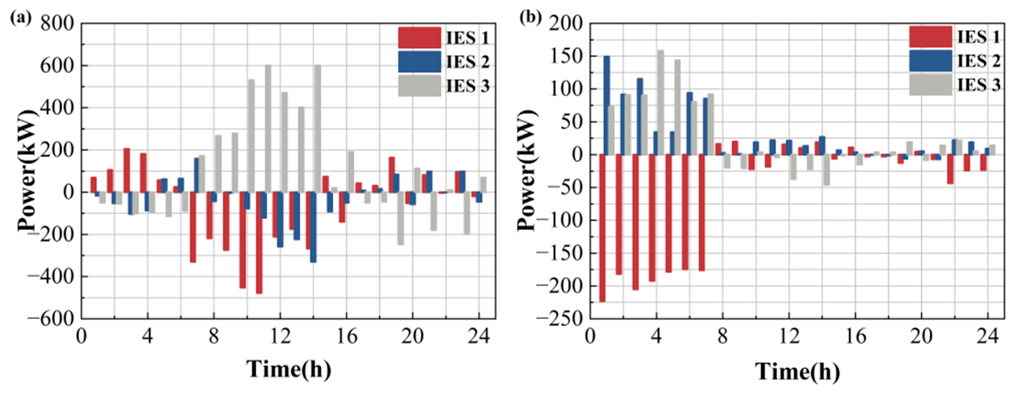
6.5. P2P Energy Trading Results

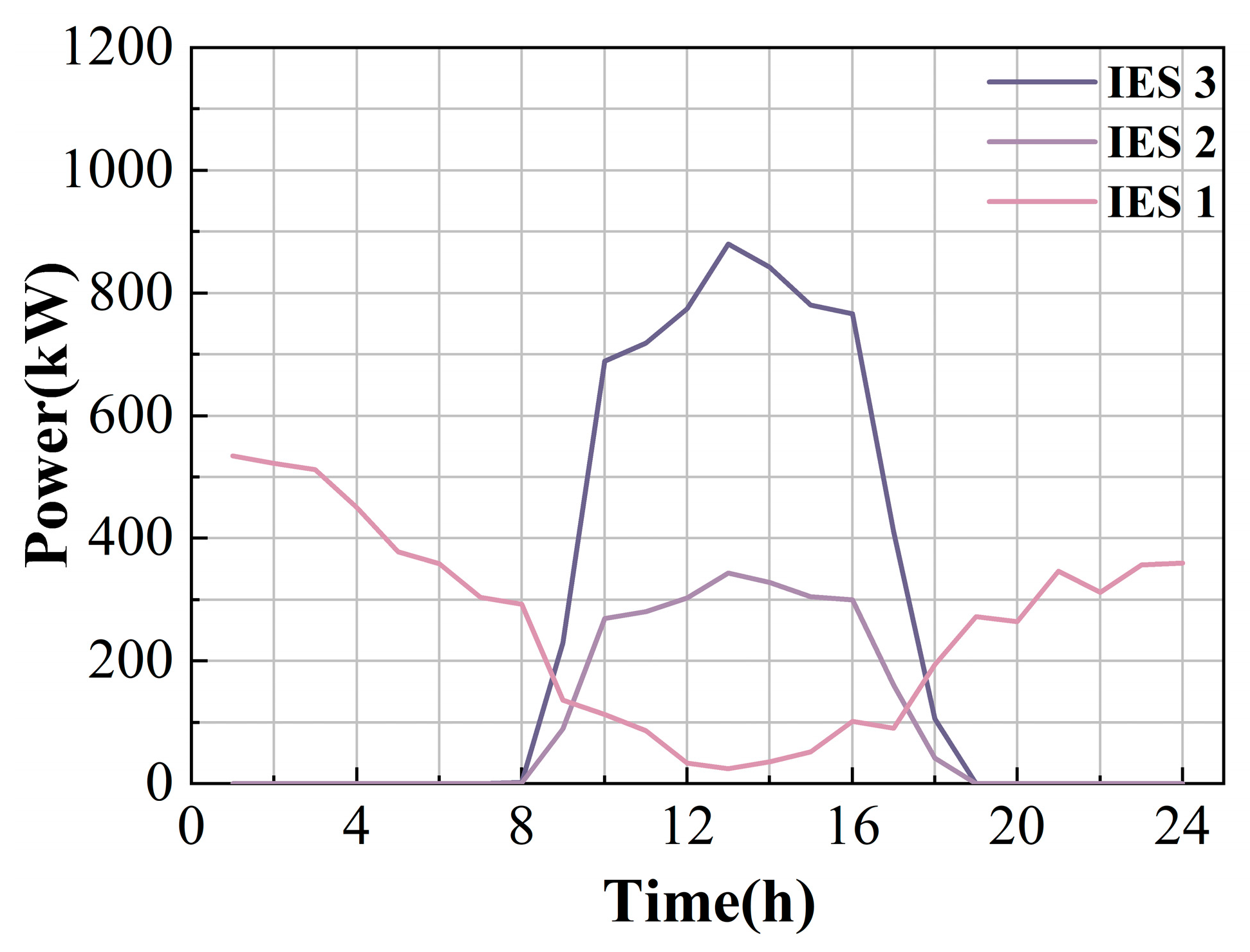
The results of the P2P electricity-heat transactions are shown in Figure 15. As seen in Figure 15a, IES 1 experienced abundant wind power generation and low electricity consumption between 00:00 and 06:00. The surplus electricity was transmitted to other IES units for profit through cooperative trading, reducing not only its own energy storage costs but also the power generation costs of other IES units. During 06:00–15:00, IES 3 experiences abundant solar power generation, while IES 1 and IES 2 face insufficient renewable generation during peak energy consumption. Consequently, IES 1 and IES 2 purchase electricity from IES 3, achieving mutual economic benefits. As shown in Figure 15b, during 00:00–07:00, IES 1 experiences high thermal demand with constrained HP power, necessitating thermal energy purchases from other IES. This demonstrates real-time energy transaction equilibrium among the three regions, highlighting the positive economic impact of P2P transactions on the IES system.

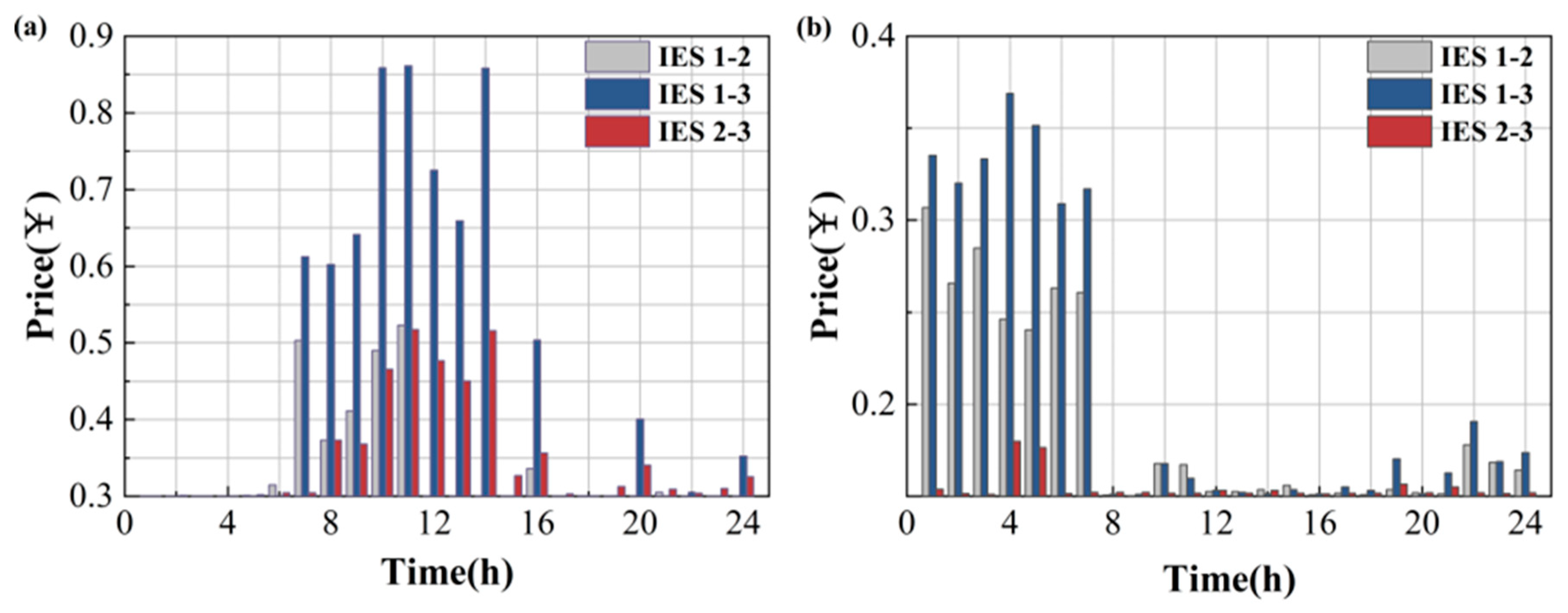
6.6. Trading Price Under Asymmetric Bargaining

As shown in Figure 16, changes in energy trading prices correspond to the energy transaction volumes depicted in Figure 15. The bargaining power of individual IESs increases with greater energy exchange, enabling them to secure more favorable transaction prices. Transaction electricity prices during each period remain within the range of the main grid’s purchase and sale prices, thereby reducing the cost of purchasing energy from the main grid and enhancing the profitability of each IES.

6.7. Revenue and Cost Analysis

Table 5. IES costs under two modes.

Mode	IES ID	P2P Pre-Trading Cost (¥)	P2P Post-Trading Cost (¥)	Final Cost (¥)	Bargaining Power (¥)	Profit (¥)
Mode 1	IES 1	13,282	11,110	12,970	0.22	312.64
	IES 2	5754	5110	5354	0.27	400.15
	IES 3	5061	6463	4359	0.51	702.29
	IES alliance	24,098	22,683	22,683	1	1415.07
Mode 2	IES 1	13,282	11,110	12,810	0.33	471.69
	IES 2	5754	5110	5282	0.33	471.69
	IES 3	5061	6463	4590	0.33	471.69
	IES alliance	24,098	22,683	22,683	1	1415.07

presents the operational costs of each IES before and after participating in P2P transactions. Mode 1 represents the proposed model in this paper, while Mode 2 corresponds to the standard Nash bargaining model.

As shown in Table 5, the asymmetric benefit allocation based on the magnitude of multi-energy contributions increases the revenues of each IES by 312.64 Yuan, 400.15 Yuan, and 702.29 Yuan, respectively, avoiding the uniform distribution of Mode 2. Therefore, the proposed benefit allocation method achieves greater rationality by considering the diverse energy contribution levels of each IES, granting higher bargaining power and profit shares to those with greater contributions.

6.8. Comparison of DRO Method Optimization Results

To further evaluate the performance of the proposed STF-CDM scenario-driven DRO method, this section compares the generated scenario sets from the proposed method with those from MC, LHS, GAN, WGAN-GP, and Diffusion models. The optimization results for the IES Alliance’s total cost and profit under different scenario sets are presented in

Table 6. Optimization results of different DRO methods.

DRO Method	IES Alliance Cost (¥)	Profit (¥)
MC	28,956	0
LHS	29,121	0
GAN	27,323	0
WGAN-GP	24,525	0
Diffusion model	23,696	402
STF-CDM	22,683	1415

. The table demonstrates that STF-CDM achieves superior total costs and profits compared to the suboptimal value. Notably, all other methods except the suboptimal one yield zero profits, validating the superior generative performance of the proposed algorithm. This reflects the lower operational costs of the STF-CDM method, confirming its accuracy and superiority.

6.9. Comparison Between Centralized Optimization and ADMM-C&CG

Table 7. Comparison between ADMM-C&CG and centralized optimization.

Algorithm	Indicator	Number of IES
		3	6	9
Centralized optimization	Cost (¥)	22,968	60,617	73,622
ADMM-C&CG	Iterations	31	39	46
	Iteration time (s)	306	527	884
	Cost (¥)	22,683	59,366	70,049

shows the optimization comparison results between the ADMM-C&CG algorithm and centralized algorithms. It can be observed that as the number of IES increases, the ADMM-C&CG algorithm achieves lower costs than centralized optimization, indicating its excellent global convergence performance. Simultaneously, the computation time of the ADMM-C&CG algorithm remains within acceptable limits, verifying the computational efficiency of the proposed method. Therefore, when the scale of IES increases, the ADMM-C&CG algorithm still exhibits good convergence performance and computational efficiency for solving the MIES cooperative operation problem.

7. Conclusions and Future Directions

This study proposes a two-stage data-driven DRO model for MIES. To more accurately capture the uncertainty in renewable energy output, a scenario generation method based on the STF-CDM is introduced to generate initial renewable energy scenarios for the DRO set. This method employs TMC and SMC units to fuse spatiotemporal features from historical data, thereby better learning the spatiotemporal characteristics of renewable energy output sequences. When handling energy transactions between MIES, the model employs multi-energy transaction contributions to allocate cooperative benefits. An ADMM-C&CG algorithm is proposed to solve this model. Meanwhile, this study offers valuable insights for energy policy formulation: It recommends promoting the development of multi-energy markets and supporting electricity-heat-cooling multi-energy trading; encouraging cloud energy storage sharing models to reduce renewable energy integration costs; and establishing a contribution-based revenue distribution mechanism to foster multi-stakeholder collaboration. These measures are envisioned to help achieve energy conservation and emission reduction targets. Key findings are as follows:

(a)

The proposed ADMM-C&CG algorithm demonstrates excellent solution performance, with each IES achieving lower cooperative operation costs than independent operation. This further mitigates the impact of renewable energy uncertainty on microgrid systems during independent operation.

(b)

When solving the energy sharing optimization model between MIES using the ADMM-C&CG algorithm, each IES exchanges only limited information, protecting IES privacy. Compared to traditional Nash bargaining models, this approach reasonably allocates cooperative benefits based on each IES’s multi-energy transaction contribution, effectively incentivizing IES entities to participate in energy transactions.

(c)

The declared STF-CDM-based DRO model reduces model conservatism compared to other scenario-driven two-stage DRO approaches.

(d)

Future research can explore hybrid game models incorporating distribution system operators and analyzing the impact of multiple uncertainties.

References

1. Guo, Y. Day-ahead optimization of integrated energy systems: A participatory dispatching approach for wind energy integration. J. Clean. Prod. 2025, 486, 144421. [Google Scholar] [CrossRef] [Scilit]
2. Li, H.; Lu, X.; Zhou, K.; Shao, Z. Distributionally robust optimal dispatching method for integrated energy system with concentrating solar power plant. Renew. Energy 2024, 229, 120792. [Google Scholar] [CrossRef] [Scilit]
3. Aliabadi, Y.; Noorollahi, Y.; Asgari, O.; Rezazadeh, M.; Moltames, R. High share of renewables in energy system planning through integration of wind energy. Energy Convers. Manag. X 2025, 26, 100899. [Google Scholar] [CrossRef] [Scilit]
4. Zhu, H.; Wang, X.; Wen, Y.; Zhu, J.; Li, J.; Luo, Q.; Liao, C. A review of integrated energy system modeling and operation. Appl. Energy 2025, 400, 126572. [Google Scholar] [CrossRef] [Scilit]
5. Ameli, H.; Pudjianto, D.; Strbac, G.; Brandon, N.P. The impact of hydrogen on decarbonisation and resilience in integrated energy systems. Adv. Appl. Energy 2025, 17, 100200. [Google Scholar] [CrossRef] [Scilit]
6. Loganathan, N.; Mayurappriyan, P.S.; Lakshmi, K.; Madhankumar, S. Robust optimization-based energy management system for integrating renewable energy resources and smart grid technology. Sustain. Energy Technol. Assess. 2025, 75, 104235. [Google Scholar] [CrossRef] [Scilit]
7. Luo, Y.; Xu, X.; Zhang, Z.; Li, P.; Hu, W.; Liu, J. A Two-Stage Robust Scheduling Optimization of an Energy Hub With Multiple Chance Constraints. IEEE Trans. Ind. Appl. 2025, 61, 1246–1255. [Google Scholar] [CrossRef] [Scilit]
8. Lv, Q.; Wang, L.; Li, Z.; Song, W.; Bu, F.; Wang, L. Robust optimization for integrated production and energy scheduling in low-carbon factories with captive power plants under decision-dependent uncertainty. Appl. Energy 2025, 379, 124827. [Google Scholar] [CrossRef] [Scilit]
9. Ma, K.; Feng, Y.; Yang, J.; Cai, Y.; Yang, B.; Guan, X. Two-stage distributionally robust optimization for port integrated energy system with berth allocation under uncertainties. Energy 2025, 322, 135588. [Google Scholar] [CrossRef] [Scilit]
10. Song, Z.; Wang, X.; Zhao, T.; Qian, T.; Zhang, L.; Qi, B.; Wang, Y. Sustainable Operation of CCUS Units Under Low-Carbon Economics. IEEE Trans. Autom. Sci. Eng. 2025, 22, 13101–13116. [Google Scholar] [CrossRef] [Scilit]
11. Rauf, A.; Kassas, M.; Khalid, M. Data-Driven Optimal Battery Storage Sizing for Grid-Connected Hybrid Distributed Generations Considering Solar and Wind Uncertainty. Sustainability 2022, 14, 11002. [Google Scholar] [CrossRef] [Scilit]
12. Shen, W.; Ding, H.; Zeng, M.; Zhang, X. Optimal bidding strategy for integrated energy system participating in spot power market: A Wasserstein metric based DRO method. Energy 2025, 327, 136402. [Google Scholar] [CrossRef] [Scilit]
13. Shi, L.; Cen, Z.; Li, Y.; Wu, F.; Lin, K.; Yang, D. Distributed Optimization of Multi-Microgrid Integrated Energy System with Coordinated Control of Energy Storage and Carbon Emissions. Sustainability 2024, 16, 3225. [Google Scholar] [CrossRef] [Scilit]
14. Zhou, Y.; Hou, H.; Yan, H.; Wang, X.; Zhou, R. Data-driven distributionally robust stochastic optimal dispatching method of integrated energy system considering multiple uncertainties. Energy 2025, 325, 136104. [Google Scholar] [CrossRef] [Scilit]
15. Ma, M.; Long, Z.; Liu, X.; Lee, K.Y. Distributionally robust optimization of electric–thermal–hydrogen integrated energy system considering source–load uncertainty. Energy 2025, 316, 134568. [Google Scholar] [CrossRef] [Scilit]
16. Yu, H.; Chen, W.; Wang, X.; Liu, D. Unsupervised Diffusion Model for Seismic Deconvolution. IEEE Geosci. Remote Sens. Lett. 2025, 22, 1–5. [Google Scholar] [CrossRef] [Scilit]
17. Liang, W.; Yang, D.; Bian, H.; Li, P. Airtightness evaluation of rubber sealing layers for compressed air energy storage cavern using the solution-diffusion model. Energy 2025, 334, 137879. [Google Scholar] [CrossRef] [Scilit]
18. Zhao, W.; Shao, Z.; Yang, S.; Lu, X. A novel conditional diffusion model for joint source-load scenario generation considering both diversity and controllability. Appl. Energy 2025, 377, 124555. [Google Scholar] [CrossRef] [Scilit]
19. Zhao, Y.; Liu, C.H.; Yi, T.; Li, G.; Wu, D. Energy-Efficient Ground-Air-Space Vehicular Crowdsensing by Hierarchical Multi-Agent Deep Reinforcement Learning with Diffusion Models. IEEE J. Sel. Areas Commun. 2024, 42, 1. [Google Scholar] [CrossRef] [Scilit]
20. Chen, C.; Liu, C.; Ma, L.; Chen, T.; Wei, Y.; Qiu, W.; Lin, Z.; Li, Z. Cooperative-game-based joint planning and cost allocation for multiple park-level integrated energy systems with shared energy storage. J. Energy Storage 2023, 73, 108861. [Google Scholar] [CrossRef] [Scilit]
21. Amiri, S.S.; Mueller, M.; Hoque, S. Investigating the Application of a Commercial and Residential Energy Consumption Prediction Model for Urban Planning Scenarios with Machine Learning and Shapley Additive Explanation Methods. Energy Build. 2023, 287, 112965. [Google Scholar] [CrossRef] [Scilit]
22. Lu, X.; Wang, C.; Sun, H.; Wang, Y.; Liu, C.; Liu, C.; Su, Y.; Cheng, R. Low-carbon Economic Dispatch of Multi-Park-Level Integrated Energy Systems Considering Thermal Network Demand Response and Improved Shapley Value Method. IEEE Trans. Ind. Appl. 2025, 1–13. [Google Scholar] [CrossRef] [Scilit]
23. Abdollahi, A.; Khavar, S.C. Enhancing the flexibility of decentralized energy resources through bi-level optimization in intra-day regional markets. Renew. Energy Focus 2026, 56, 100778. [Google Scholar] [CrossRef] [Scilit]
24. Song, Z.; Cao, S.; Yang, H. An interpretable framework for modeling global solar radiation using tree-based ensemble machine learning and Shapley additive explanations methods. Appl. Energy 2024, 364, 123238. [Google Scholar] [CrossRef] [Scilit]
25. Li, H.; Han, Y. Data-driven distributionally robust collaborative optimization operation strategy for a multi-microgrid based on LSTM-CGAN. Dianli Xitong Baohu Yu Kongzhi Power Syst. Prot. Control. 2024, 52, 133–148. [Google Scholar]
26. Chen, L.; He, S.; Fan, X. Cooperative optimization of shared energy storage in integrated energy systems using adaptive ADMM and Nash bargaining. J. Energy Storage 2025, 134, 118148. [Google Scholar] [CrossRef] [Scilit]
27. Huang, C.; Ge, Z.; Wang, L.; Zhang, D.; Long, H.; Luo, X. Multi-Agent Deep Reinforcement Learning-Based Cooperative Optimal Operation for Building Integrated Energy Systems With Nash-Harsanyi Bargaining Game-Driven Cost Allocation. IEEE Trans. Consum. Electron. 2025, 71, 4759–4770. [Google Scholar] [CrossRef] [Scilit]
28. Zhang, K.; Chen, J.; Qi, X.; Zhang, W.; Wei, M.; Lin, D. Cooperative optimal operation of multi-microgrids and shared energy storage for voltage regulation of distribution networks based on improved Nash bargaining. Int. J. Electr. Power Energy Syst. 2025, 166, 110532. [Google Scholar] [CrossRef] [Scilit]
29. Zhu, X.; Liu, S.; Cao, Y.; Zhang, Y. An asymmetric Nash bargaining based day-ahead distributed energy sharing strategy for integrated energy service providers. Int. J. Electr. Power Energy Syst. 2025, 169, 110744. [Google Scholar] [CrossRef] [Scilit]
30. Purage, M.I.S.L.; Krishnan, A.; Foo, E.Y.S.; Gooi, H.B. Cooperative Bidding-Based Robust Optimal Energy Management of Multimicrogrids. IEEE Trans. Ind. Inform. 2020, 16, 5757–5768. [Google Scholar] [CrossRef] [Scilit]
31. Wu, B.; Zhang, S.; Yuan, C.; Wang, X.; Wang, F.; Zhang, S. Cooperative energy and reserve trading strategies for multiple integrated energy systems based on asymmetric nash bargaining theory. Energy 2024, 313, 133703. [Google Scholar] [CrossRef] [Scilit]
32. Ahmad, Z.; Shukla, A.K.; Singh, V.; Sharma, M.; Kumar, P. Thermodynamic analysis of solar powered trigeneration arrangement for cooling, power and drinking water generation. Songklanakarin J. Sci. Technol. 2022, 44, 1419–1426. [Google Scholar]
33. Bagherian, M.A.; Mehranzamir, K.; Pour, A.B.; Rezania, S.; Taghavi, E.; Nabipour-Afrouzi, H.; Dalvi-Esfahani, M.; Alizadeh, S.M. Classification and Analysis of Optimization Techniques for Integrated Energy Systems Utilizing Renewable Energy Sources: A Review for CHP and CCHP Systems. Processes 2021, 9, 339. [Google Scholar] [CrossRef] [Scilit]
34. Xing, Z.; Feng, Q.; Chen, H.; Dai, Q.; Hu, H.; Xu, H.; Wu, Z.; Jiang, Y.-G. A Survey on Video Diffusion Models. ACM Comput. Surv. 2025, 57, 1–42. [Google Scholar] [CrossRef] [Scilit]
35. Zhang, Y.; Ding, Y.; Xie, H.; Zhang, S.; Xu, H.; Cao, L.; Huang, Z. TransDiff: Transformer-based diffusion model for low-light image enhancement. Neurocomputing 2025, 655, 131174. [Google Scholar] [CrossRef] [Scilit]
36. Chen, L.-Y.; Kao, M.; Chen, S.-H.; Yang, C.-H. A Diffusion-Model-Based Methodology for Virtual Silicon Data Generation. IEEE Trans. Semicond. Manuf. 2025, 38, 146–153. [Google Scholar] [CrossRef] [Scilit]
37. Zhou, P.; Wang, W.; Lin, D.K.J.; Liu, Y. A novel criterion based on continuous ranked probability score for performance evaluation of control charts. Qual. Reliab. Eng. Int. 2023, 39, 2081–2093. [Google Scholar] [CrossRef] [Scilit]
38. Lambert, D.; Jarrin, T.; Richard, N.; Duhamel, O.; Paillet, P. Monte Carlo simulations: From neutron to defects in bulk materials. IEEE Trans. Nucl. Sci. 2025, 72, 2519–2526. [Google Scholar] [CrossRef] [Scilit]
39. Gao, S.Q.; Zhao, H.; Cheng, J.-Y.; He, Q.-Q.; Mao, J.-D.; Rao, Z.-M.; Zhou, C.-Y.; Gong, X. Simultaneous Inversion of the Complex Refraction Index and the Particle Size Distribution of Nonspherical Aerosol Particles Using Latin Hypercube Sampling Method. IEEE Trans. Geosci. Remote Sens. 2025, 63, 4107915. [Google Scholar] [CrossRef] [Scilit]
40. Ozsipahi, M.; Jean, S.; Beskok, A.; Wilson, A.A. Molecular dynamics simulation of thermal conductivity of GaN. Int. Commun. Heat Mass Transf. 2025, 163, 108658. [Google Scholar] [CrossRef] [Scilit]
41. Zuo, J.; Lei, M.; Wang, S.; Dong, S.; Li, W. Augmented deep transfer learning for SRP condition monitoring via physically-informed WGAN-GP approach. Meas. Sci. Technol. 2025, 36, 016028. [Google Scholar] [CrossRef] [Scilit]
Figure 1. MIES optimization framework.
Sustainability 17 11377 g001
Figure 2. The MIES operational model framework.
Sustainability 17 11377 g002
Figure 3. The internal system model of the IES.
Sustainability 17 11377 g003
Figure 4. The network architecture of the STF-CDM.
Sustainability 17 11377 g004
Figure 5. ADMM-C&CG algorithm flowchart.
Sustainability 17 11377 g005
Figure 6. Raw data for renewable energy sources.
Sustainability 17 11377 g006
Figure 7. Energy prices.
Sustainability 17 11377 g007
Figure 8. Renewable energy scenarios for each IES. (a) IES 1; (b) IES 2; (c) IES 3.
Sustainability 17 11377 g008
Figure 9. Test metric results for the CDM in IES 1 and IES 2. (a) MAE; (b) RMSE; (c) CRPS; (d) FID.
Sustainability 17 11377 g009
Figure 10. The convergence characteristics of the proposed parallel ADMM-C&CG algorithm when solving Subproblem 1. (a) ADMM distributed iterative curve; (b) Convergence plot of the C&CG algorithm for IES 1; (c) Convergence plot of the C&CG algorithm for IES 2; (d) Convergence plot of the C&CG algorithm for IES 3.
Sustainability 17 11377 g010
Figure 11. ADMM solution cost iteration process. (a) IES 1; (b) IES 2; (c) IES 3.
Sustainability 17 11377 g011
Figure 12. Power load balance of IES 1. (a) Electrical load balance; (b) Thermal load balance; (c) Cooling load balance.
Sustainability 17 11377 g012
Figure 13. Power load balance of IES 2. (a) Electrical load balance; (b) Thermal load balance; (c) Cooling load balance.
Sustainability 17 11377 g013
Figure 14. Power load balance of IES 3. (a) Electrical load balance; (b) Thermal load balance; (c) Cooling load balance.
Sustainability 17 11377 g014
Figure 15. Energy trading results between IES. (a) Electricity trading; (b) Thermal trading.
Sustainability 17 11377 g015
Figure 16. Energy trading prices between IES. (a) Electricity trading; (b) Thermal trading.
Sustainability 17 11377 g016