End-to-End Modelling as a Non-Invasive Tool for Sustainable Risk Management After the Rupture of the Landslide Dam Along River Courses

Abstract

Debris flows represent a significant geohydrological hazard, impacting the surrounding environment and threatening human settlements by altering ecological equilibria. The formation of temporary, often unstable, natural dams that obstruct normal river flow and create secondary flood risks poses a complex and prolonged threat to the sustainable management of water resources. Non-invasive risk assessment and analysis tools are therefore essential for addressing this challenge effectively. In this context, this study uses an end-to-end numerical modelling approach validated on an actual river obstructed in past by a debris flow. The simulation focused on sustainable risk management after the landslide dam rupture. This computational methodology is a non-invasive technology that provides a fundamental alternative to costly and environmentally invasive field techniques for assessing the risk of complex river systems. Two separate numerical simulations were carried out using the HEC-RAS code. The first simulation used the integrated sediment transport module to quantify the dynamics of solid material deposition and dilution. The second simulation modelled secondary flooding scenarios using the dam break simulation module. The aim of integrating these non-invasive simulations is to analyse the interaction between the river and debris accumulation, understand the river’s natural regeneration capacity and determine the hydraulic response to sudden dam failure. These results are essential for geohydrological risk assessment and mitigation, thereby improving the effectiveness of prevention measures and systemic resilience against landslides.

1. Introduction

Debris flows are gravity-driven flows consisting of a dense mixture of water, sediment, mud, and in some cases, large rock blocks [1]. Their velocity depends on the topography and obstacles along the slope, and it is often very high. In confined channels, the limited space can increase both the velocity and pressure of the flow, giving it particularly disruptive properties and the capacity to alter the surrounding landscape, dam rivers, or damage human structures and infrastructures [2]. One of the major risks associated with debris flows in river contexts is that the possibility that the sediment load introduced by the flow may exceed the river’s transport capacity at the confluence with the main channel. If this occurs the debris flow may deposit a significant amount of material, which could lead to the formation of temporary natural dams within the riverbed [3]. Specifically, in the Italian Alpine and Apennine contexts, the topography can cause these temporary barriers and can lead to a sudden break. Such failures can generate secondary flood waves that spread quickly and cause extensive damage. One of the most devastating historical events of this type of risk is the collapse of the dam on the Dadu River in Sichuan, which occurred on 10 June 1786, ten days after an earthquake that caused the landslide. Thousands of people were killed by a flood wave that travelled more than one thousand four hundred kilometres [4]. Developing state-of-the-art numerical models is essential for accurately simulating the dynamic interaction between rivers and debris flows [5,6]. This is an indispensable step in an effective quantitative risk assessment. These models predict the path and velocity of the flow and the erosion and deposition processes that occur during the event [7]. The existing studies on debris-flow dynamics, sediment transport, dam formation, and consequent failure, focus on the processes separately, limiting the interpretation of their coupled behavior within river systems [8,9]. Additionally, the increasing frequency and intensity of such events under climate-driven rainfall extremes highlights the urgency of integrated risk assessment tools [10], example are the Matagida Creek and the barrier-lake overflow alert that led to the closure of Taroko National Park [11,12]. This study addresses these gaps by employing an end-to-end modelling approach that combines debris-flow propagation, sediment transport, and dam-break simulations within a single framework, providing a comprehensive perspective on river response and potential secondary flooding [10,13]. This work focuses on investigating the complex interactions between debris flows and the riverbed, particularly the formation of temporary dams in the main channel through the simulation of non-Newtonian flow dynamics, and their influence on river conditions. The study also examines the potential consequences of dam failure, including secondary flooding events and alterations to the river’s hydrology [14,15]. These dams, often formed by a sudden inflow of debris, can drastically modify the river’s hydraulic and morphological regime, with severe consequences for both the environment and people. This can cause potential flooding upstream, and if the dams collapse, it can trigger catastrophic flooding downstream, resulting in dramatic changes to the channel’s morphology. The study is based on an end-to-end approach, which is useful for gaining a complete and integrated perspective of the phenomena [16]. This provides a comprehensive understanding of how the mechanisms governing debris flow propagation, sediment accumulation, and river flow dynamics interact with each other. Currently, debris flow propagation and sediment transport are predominantly modelled as separate phenomena, with limited consideration of their coupled dynamics [17]. An end-to-end [18] approach can be used to model both process simultaneity and their interaction over time and space. This includes the potential formation and subsequent failure of temporary debris dams, which can trigger secondary flooding and significantly impact conditions in the downstream river [19]. In this work, two scenarios of simulations were carried out using the HEC-RAS software v6.6 (i) with the specific tool for assessing sediment transport [20] (ii) with the specific module designed for the dam failure. The first series of simulations focuses on the propagation of the debris flow and its impact on the Liri River. The initial discharge was estimated from rainfall data using the SCS-CN method and then converted into debris flow discharge using the Gregoretti and Della Fontana (2008) formula [3]. The second series of simulations was based on flow data from the Liri River recorded at the Civitella Roveto (AQ) hydrometric station covering the period around the debris flow reactivation. These data are crucial for understanding the hydrological conditions that led to the event, such as increased soil pore pressure and slope erosion [21]. The simulations analyse what happens when the flow reaches the river, which can lead to the formation of temporary dams, increased sediment transport and significant changes in river hydraulics. The results highlight the locations and times at which the river’s transport capacity is exceeded that can potentially increase the risk of flooding both upstream and downstream. The results indicate that, while temporary debris dams can form and locally alter flow conditions, the effects are generally confined to areas immediately upstream of the blockage. The peak flow gradually decreases downstream, and the river tends to return to uniform conditions after the event has passed. Even in the most severe scenarios, the simulations suggest that a dam failure would not result in widespread flooding or a significant increase in hydraulic risk along the riverbed. This highlights the river’s ability to handle such events without causing major impacts on the surrounding areas. Additionally, the model effectively illustrates how long it takes for the river to restore sediment transport equilibrium and where sediment deposition is likely to occur. Together, these simulations provide a comprehensive view of the event, from its origin to its consequences. The study is structured to provide a clear and comprehensive understanding of debris-flow impacts on the Liri River. It begins with simulations of debris deposition using the integrated sediment transport module in HEC-RAS [22], allowing identification of areas where sediment accumulates and the river’s capacity to transport debris downstream. Following a second set of simulations uses the dam-break module, included in the code, was used to assess potential secondary flooding scenarios and the river’s response to sudden failure of temporary debris dams. By integrating these simulations within a single framework, the study captures the interactions between debris-flow processes, sediment dynamics, and river hydraulics, offering a complete depiction of the event—from its initiation on the slopes to the downstream impacts at the Liri River confluence. This approach defines the methodological backbone of the work and provides a coherent framework for the analyses and discussions that follow. By combining sediment transport and dam-break simulations within a single model, it enables the development of sustainable water resource management strategies and the protection of riverine ecosystems. Furthermore, modelling outcomes facilitate the evaluation and mitigation of geohydrological risks in mountainous catchments, thereby enhancing preparedness and resilience against landslide hazards. The results highlight differences in Liri River discharge under natural conditions compared to after debris flow events occur, as well as the impact of dam breaks on the surrounding landscape. These findings provide valuable insights into sediment dynamics and the processes triggered by debris flow events.

2. Study Area

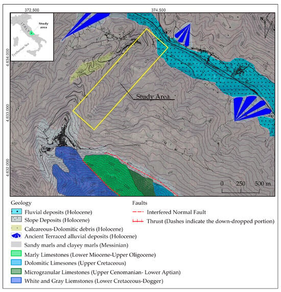
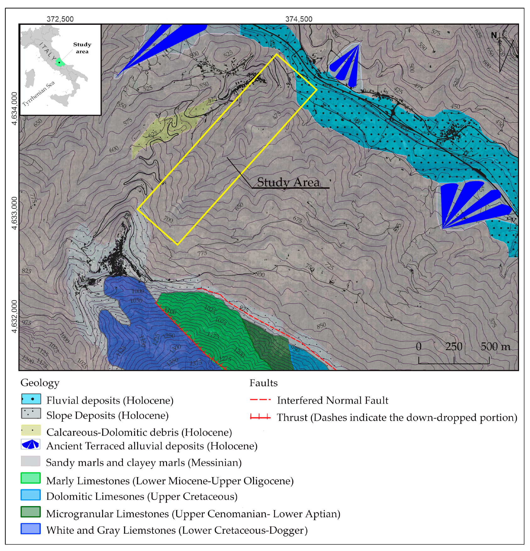
Rendinara hamlet is in the upper Roveto Valley, an Apennine valley of Italy that stretches along the upper stream of the Liri River. The landslide extends 2600 m. from the head to the tail of the phenomenon and has a width of 920 m [23], indicating a significant dimension and the potential for large volumes to be involved. Landslide materials, according to the local geology, consist mainly of boulders and carbonate debris in an abundant clay matrix (Figure 1). This landslide begins in the upper sector of the study area, where highly tectonized carbonate rocks dominate [24,25]. In this context, tectonic stress is a predisposing factor for the local instability of the rock mass, generating multiple rockfalls and avalanches [26]. In this sector, major evidence includes several blocks found in the upper sector of slope, highly fractured rocks recorded during the field activity and significant slope debris accumulated at the base of the unstable rock sector [27,28,29]. Along the slope, due to the presence of debris materials with different permeability and grain size, springs are formed and fed by carbonate aquifer, which in turn is replenished by rainwater; therefore, these springs have variable flow rates depending on the season. The last reactivation of analysed phenomena in this study was triggered in March 2021; the days leading up to the event were, on average, wetter than usual, with approximately 756 mm of rain concentrated over 15 days, averaging about 50 mm per day [30]. From the hydrogeological point of view, the area is characterized by the presence of a regional aquifer, marked by the detrital cover and flysch deposits, as well as a carbonate aquifer formed by limestones and dolomitic limestones, locally highly fractured.

Due to the dismantling caused by the active tectonic regime and given the steep slope of the upper part of the slope, the fractured and dismantled limestones tend to form numerous and varied deposits that blanket the flysch lithologies [31,32,33,34]. The massive deposit produced by this unstable sector forms an unstable cover layer over the marls composing the central sector of the slope. These deposits are highly heterogeneous due to the alternating materials [25,35,36,37]. In the central sector, there are major geomorphological features such as trenches, secondary scarps, and significant cracks. These elements are sometimes concealed by geomorphological signatures related to active tectonic stress, as evidenced by the ribbon-shaped slope on the right side and the emergence of several springs on the slope, especially after prolonged rainfall periods. These deposits are extremely heterogeneous and; therefore, within them, they tend to form layers with different permeability.

3. Materials and Methods

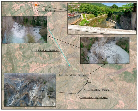
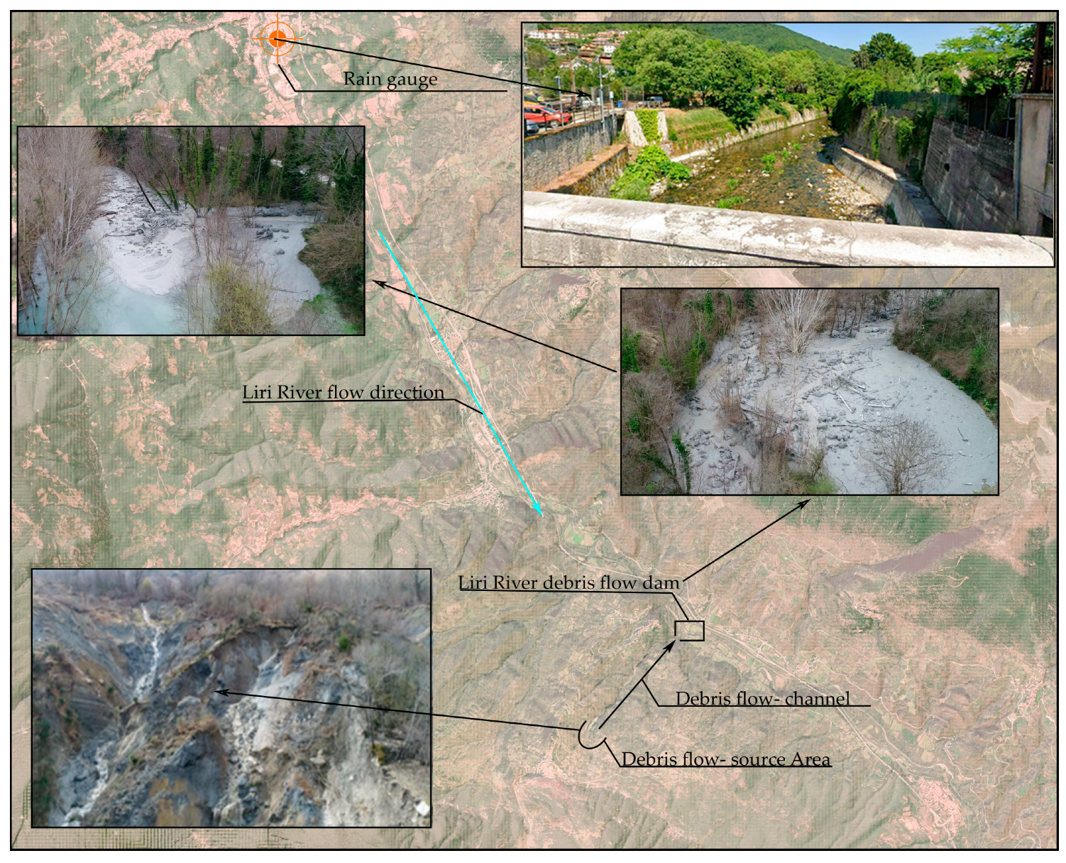
To provide an integrated representation of the debris flow dynamics propagation and its interaction with the riverbed, simulations were performed using HEC-RAS code v.6.6. This analysis was made possible by combining use of the sediment transport module and the tool designed specifically for analysing temporary dam failure. The model used for the analysis was calibrated using hydrological values, rainfall data and morphological surveys of the Liri River basin (Figure 2).

This process was allowed to the reconstruction of the flow conditions debris accumulation processes, and potential scenarios of temporary dam failure. To determine the impact of debris flows on the Liri river, two separate simulation series were conducted: (1) debris flow impact and (2) dam break.

3.1. Rio Sonno Debris Flow Impact on Liri River

The first simulation scenario focuses on the impact of debris flowing into the Liri River via the Rio Sonno tributary. The debris flow simulation was performed using the Debris Flow Library implemented within the HEC-RAS v6.6 software, which extends the standard hydrodynamic solver to account for non-Newtonian flow behavior typical of sediment-laden and viscous mixtures. The model numerically solves the modified Shallow Water Equations, incorporating rheological parameters such as yield stress and dynamic viscosity to represent the complex interactions between solid and fluid phases during debris flow propagation. This allowed the combined effects of both phenomena to be assessed. This dual approach enables a direct comparison of river conditions with and without debris flow to be made, providing a comprehensive assessment of its impact [38]. To analyze the interaction between the river and the debris flow event, the first step was to determine the Liri flow rate based on data from the hydrometric station closest to where the event occurred. This regional monitoring station is identified by the code N005LR8 and is located at the coordinates 41.935081° N, 13.418529° E. Direct measurements of the Liri River’s flow rate during the period immediately before and during the debris flow were extracted from the monitoring network database.

A basic hydraulic model was constructed using the HEC-RAS code to simulate the behavior of the river under natural flow conditions, improving our understanding of it in the process. This model enabled the initial hydraulic conditions of the Liri River to be reconstructed prior to the event, providing a realistic context in which to evaluate the impact of the debris flow on river dynamics. A debris flow occurs when loose material, such as sediment, rocks and debris, interacts with enough water to transform the flow into a highly concentrated mixture of water and solids. In this study, the debris flow hydrograph was estimated using the formula of Gregoretti and Della Fontana [3]. They obtained the critical discharge relationship using flume-laboratory data for debris flow initiation [39], following the approach of Tognacca et al. [40]. This formula depends on the mean grain size of the sediments and the angle of the bed slope (see Equation (1)).

$$q_{critic}=0.78·D_M^{1.5}·\tan \left(\vartheta \right)-1.27$$

(1)

where $q_{critic}$ is the critical discharge per unit width (${\mathrm{m}}^2/\mathrm{s}$), $D_m$ is the mean grain size, and ϑ is the bed slope.

A debris flow is triggered when the runoff discharge $q_r$ exceeds the critical threshold $q_{critic}$, which is calculated by multiplying the critical unit discharge by the channel width in the triggering section. Discharge was calculated using the Soil Conservation Service (SCS) method [41,42] to derive the debris flow. This method facilitates the generation of synthetic unit hydrographs (SUHs). SUHs are theoretical hydrographs that represent a watershed’s direct runoff response to a unit of effective rainfall over a specified duration. The SCS method uses a dimensionless reference curve to predict the shape of SUHs. This curve relates time and flow ratios quantitatively [43,44]. Specifically, the time ratio is usually defined as the time from the start of the excess rainfall to the peak of the hydrograph, while the flow ratio is defined as the discharge at a given time divided by the peak discharge. This dimensionless approach enables the method to be applied to watersheds of various sizes and characteristics. The foundational principle of the method is represented by the following relationship (Equation (2)):

$$Q={\displaystyle \frac{{\left(P-I_a\right)}^2}{P-I_a+S}} per P> I_a$$

(2)

where $Q$ is the runoff (mm), $P$ is the total rainfall (mm), $I_a$ is the initial abstraction (mm), accounting for interception, surface storage, and infiltration prior to runoff and $S$ is the maximum potential soil moisture retention after runoff begins (mm).

A common relation between $I_a$ e $S$ is typical $I_a=0.2·S$. This implies that, on average, 20% of the soil’s potential retention capacity is lost through initial abstraction before direct runoff begins. The parameter S can then be expressed in terms of the Curve Number (CN) and it is equal to (Equation (3)):

$$S=S_0({\displaystyle \frac{100}{CN}}-1)$$

(3)

The Curve Number (CN) ranges from 30 (high infiltration, low runoff) to 100 (low infiltration, high runoff), and it depends on land use, hydrologic soil group (HSG), and antecedent moisture conditions (AMC). Four hydrologic soil groups are defined, from A to D with an infiltration ratio growing from D to A. Once the HSG is identified, the CN is determined according to land use. CN is further adjusted based on antecedent moisture conditions (AMC), which reflect soil saturation prior to the event, the AMC is divided in three classes from I, that represents the dry condition to III that indicate saturated conditions [45,46,47]. Statistically, AMC I, II, and III correspond to exceedance probabilities of 90%, 50%, and 10%, respectively, in terms of runoff depth for a given rainfall event [41]. The synthetic unit hydrograph [47] is constructed by using the ratios of discharge (Q) to peak discharge (Q_p), and time (t) and time to peak (t_p). Initially, as rainfall contributes to runoff, the Q/Q_p ratio progressively increases, signifying the rising phase of the hydrograph. This step continues until the maximum value of 1 is reached which occurs at the point of peak discharge Q_p and the time t_p. After this point the ratio Q/Q_p begins to decrease back toward zero, defining the hydrograph’s shape and duration.

Different methods can be used to determine the peak discharge Q_p, relating watershed characteristics to the runoff response. For ungauged watersheds where direct measurements are unavailable, Mockus [48], suggests calculating the peak flow rate as follows (Equation (4)):

$${\mathrm{Q}}_{\mathrm{p}}={\displaystyle \frac{0.208\times \alpha \times Q}{{\mathrm{t}}_p}}$$

(4)

where $\alpha$ is the catchment area (km²), while $Q$ represents the runoff (mm).

The time to peak (${\mathrm{t}}_p$) expressed in hours, was estimated as a fraction of the basin concentration time, based on the SCS-CN method. This approach simplifies the process of estimating hydrograph rise time by focusing on catchment response characteristics. The unit hydrograph is used to create runoff hydrographs. This process incorporates cumulative rainfall data determined from IDF curves for various return periods. To address the uncertainty arising from the spatial concentration of meteorological events, we identify three different contributing areas where the topographic analysis is performed in a GIS environment. Specifically, we apply an eight-direction poor point algorithm to the region’s digital elevation (DEM) and drainage network to delineate the watershed. Starting from the SCS hydrograph, the debris flow hydrograph was derived using the formulation proposed by Gregoretti and Della Fontana 08, assuming the initial sediment volume as estimated by [49]. The time of concentration (${\mathrm{t}}_c$) was defined as 0.173 h and the peak discharge (${\mathrm{Q}}_{\mathrm{p}}$) as 33.87 m³/s, based on the main characteristics of the unit hydrograph, to describe the sub-basin’s response time to a rainfall input of 62 mm over two hours. Sediment dynamics were implemented by [3], while the channel bottom width was estimated through analysis of high-resolution digital imagery and a 1 × 1 m Digital Terrain Model (DTM). The HEC-RAS code is used to simulate various inundation scenarios. This involved applying shallow water equations [50,51], which are fundamental to modelling fluid flow. To enhance these simulations, we used the Debris-Lib extension, which was developed by Gibson in [20]. This numerical library allows for the simplified simulation of granular flow dynamics and provides a more comprehensive understanding of how debris might interact with floodwaters. The shallow water equations were chosen because they can represent the propagation of flows in steep channels while maintaining computational stability. While this approach does not consider local acceleration or super-elevation effects, it offers an effective balance between model accuracy and numerical performance for this type of application [36,37]. The simplified Bingham model was selected to represent the internal resistance of the debris flow in the Rio Sonno basin, which features heterogeneous sediments and significant clay content. While it does not capture local acceleration or turbulence, it provides a robust first-order approximation suitable for assessing the flow impact on river hydraulics. Despite its limitations, the choice allows for first-order approximation of internal resistance in such flows. The parameters governing the mixture’s behavior were set using default or literature-based values, with an assumed internal friction angle of 30°, which is consistent with that of typical debris flow material. Inflow was introduced at the bottom of the source area, identified as a single sub-basin in line with the assumptions of the SCS method. Sediment characteristics derived from field analyses were introduced in the software dedicated section. Furthermore, the thickness of the sediment layer was estimated using geophysical surveys conducted in the area. The sediment transport equations were then selected according to the grain-size properties of the debris source basin. Attention was given to the presence of clay and the highly heterogeneous grain size distribution resulting from the weathering of detrital aquifer materials upstream [52]. The fall velocity of individual particles was calculated using the Soulsby formula [53], which provides an accurate estimate considering sedimentological heterogeneity.

$$w_s={\displaystyle \frac{v}{d}}\left[{\left({\displaystyle \frac{1}{{0.36}^2}}+1.049·{{(d}^{\ast })}^3\right)}^{1/2}-{\displaystyle \frac{1}{0.36}}\right]$$

(5)

where $w_s$ is the fall velocity of the sediment (m/s), $v$ is the kinematic viscosity of water (m²/s), $d$ is the grain size, $d^{\ast }$ is the dimensionless grain size, calculated us $d^{\ast }=d{\left[{\displaystyle \frac{(s-1)·g}{v^2}}\right]}^{1/3}$ where $s$ is the specific density (or relative density) of the sediment and $g$ is the gravitational constant.

Given the significant clay content and the wide variability in grain size, a hybrid approach was adopted rather than relying on a single total-load formula. The non-cohesive fraction (particles > 63 µm) was modelled using the Van Rijn formulations [53] for bedload and suspended load.

$$q_b=0.053{\displaystyle \frac{\sqrt{\left(s-1\right)g{D}_{50}^3}}{D_{\ast }^{0.3}}}\hspace{0.17em}{T}^{2.1}$$

(6)

$$q_s=0.012{\displaystyle \frac{\sqrt{\left(s-1\right)g{D}_{50}^3}}{D_{\ast }^{0.6}}}\hspace{0.17em}{T}^{2.4}$$

(7)

where $q_b$ and $q_s$ are the bed-load and suspended-load transport rates per unit width, respectively; $s={\rho }_s/\rho$ is the relative density; $g$ is the acceleration due to gravity; $D_{50}$ is the median grain size; $D_{\ast }$ is the dimensionless particle size; and $T=({\tau }_b-{\tau }_{cr})/{\tau }_{cr}$ the dimensionless excess shear stress. For bedload of mixed/poorly sorted surface materials (where sand/gravel interactions are important) surface-based fractional bed-load formulation was used as a sensitivity check [54,55]. Total sediment fluxes were computed by summing the contributions of the non-cohesive bedload and suspended-load and the cohesive erosion/deposition fluxes; hiding/exposure corrections and limits on near-bed concentration were applied where required. This hybrid scheme follows common practice for rivers with mixed sand–silt–clay compositions. Using these models together allowed us to consistently regulate sediment transport in line with the physical and morphological properties of the sediments, while maintaining numerical stability and an appropriate level of detail in describing the phenomena [25,36].

Two different scenarios were simulated:

• Base flow scenario: discharge of the Liri River only, to assess typical flow conditions.
• Combined flow scenario: simultaneous discharge of the Liri River and debris flow, to evaluate the impact of extreme events on sediment transport.

3.2. Dam Break Simulation

The dam break simulation was carried out using the two-dimensional unsteady flow module of the HEC-RAS v6.6 code. This approach solves numerically the Shallow Water Equations (Saint-Venant equations) for unsteady free-surface flow [56]. The conservation of mass and momentum are described as:

$${\displaystyle \frac{\partial h}{\partial t}}+{\displaystyle \frac{\partial \left(uh\right)}{\partial x}}+{\displaystyle \frac{\partial \left(vh\right)}{\partial y}}=q$$

(8)

$${\displaystyle \frac{\partial \left(uh\right)}{\partial t}}+{\displaystyle \frac{\partial }{\partial x}}(u^{2}h+{\displaystyle \frac{1}{2}}g{h}^2)+{\displaystyle \frac{\partial \left(uvh\right)}{\partial y}}=gh(S_{0}x-S_{fx})$$

(9)

$${\displaystyle \frac{\partial \left(vh\right)}{\partial t}}+{\displaystyle \frac{\partial }{\partial y}}(v^{2}h+{\displaystyle \frac{1}{2}}g{h}^2)+{\displaystyle \frac{\partial \left(uvh\right)}{\partial x}}=gh(S_{0}y-S_{fy})$$

(10)

where $h$ is the water depth (m), $u$ and $v$ are the depth-averaged velocity components (m/s) in the longitudinal and transverse directions, respectively, $S_0$ is the bed slope, $S_f$ is the friction slope (computed using Manning’s formula) and $q$ is the lateral inflow per unit area (m/s).

The computational domain was defined as a 2D Flow Area covering the valley reach of the Liri River affected by the natural blockage and subsequent flood wave propagation. The LiDAR data (1 × 1 m resolution, provided by the Italian Ministry of Environment) was used to generate a high-resolution terrain model, allowing accurate representation of the valley morphology and the temporary reservoir formed upstream of the landslide dam [56]. A computational mesh with regular cells of 10 × 10 m was adopted, with local refinement to 3 × 3 m in the dam area to accurately capture the breach geometry and flow transitions. Break-lines were used to refine the mesh along morphological discontinuities, ensuring topographic adherence without excessive refinement. The temporary reservoir upstream of the dam was modelled as a Storage Area (SA), characterized by a Volume–Elevation curve derived by the DTM. The SA is connected to the river domain by a Storage Area Connection, which represents the natural dam section and its potential failure mechanisms. A small culvert was added to simulate a continuous low-flow drainage through the landslide deposit. This was calibrated based on field observations. The dam break was modelled using the Froehlich’s empirical formulation [57,58], which estimates the final breach width and formation time based on the reservoir volume and the depth of the water upstream. This approach was chosen as a conservative assumption to simulate the maximum possible outflow peak [59]. Different simulation scenarios were tested to account for varying initial and hydrological conditions:

• Pure dam break: empty channel, full reservoir, no inflow.
• Low flow (≈8 m³/s): initial discharge through the culvert followed by moderate inflow.
• High flow (≈80 m³/s): breach formation during peak flow conditions.

For all simulations, upstream inflow was imposed as a Lateral Inflow Hydrograph on the storage area, while downstream boundary conditions were defined as normal depth. Initial steady-state conditions were obtained by running a short pre-simulation with a constant discharge of 1.75 m³/s to establish low-flow conditions in the channel prior to breach initiation. The unsteady flow computations used an implicit finite-volume scheme with θ-weighting = 1.0 (fully implicit backward Euler integration) to ensure numerical stability under rapidly varying flow condition [59]. The adaptive time step was automatically adjusted based on the Courant number, maintained between 0.4 and 1.0, with a base step ranging from 0.2 to 0.4 s. The Pardiso direct solver was adopted for the linear system solution, allowing up to 30 iterations per time step with strict convergence tolerances (Δh ≤ 0.003 m; volume error ≤ 0.3%). A conservative turbulence model was applied, with mixing coefficients of 0.3 (longitudinal), 0.1 (transverse), and a Smagorinsky coefficient equal to 0.05 [60,61,62]. Hydrological data were obtained from the Civitella Roveto hydrometric station, including hourly and daily water level readings for March 2021 (period the debris flow occurred, blocking the river downstream). Discharge values [63] were estimated from stage readings using a simplified Gauckler–Strickler equation for a rectangular channel of width 17.45 m, bed slope $i_f=0.003$, and roughness coefficient $k_s=60\hspace{0.17em}{\mathrm{m}}^{1/3}/\mathrm{s}$ [50].

$$Q=k_s\hspace{0.17em}A\hspace{0.17em}{R}^{2/3}\hspace{0.17em}\sqrt{i_f}$$

(11)

where $A$ is the wetted area (m²) and $R=A/P$ is the hydraulic radius (m).

Model calibration was performed using measured water levels and inferred discharges to ensure consistency between simulated and observed flow dynamics.

4. Results

This section presents the main results of the hydrodynamic and sediment transport simulations, with a specific focus on the effect of the Rio Sonno debris flow on the hydraulic and sedimentological conditions of the Liri River.

4.1. Debris Flow Interaction with the Liri River

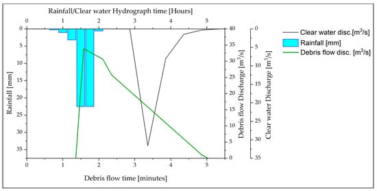
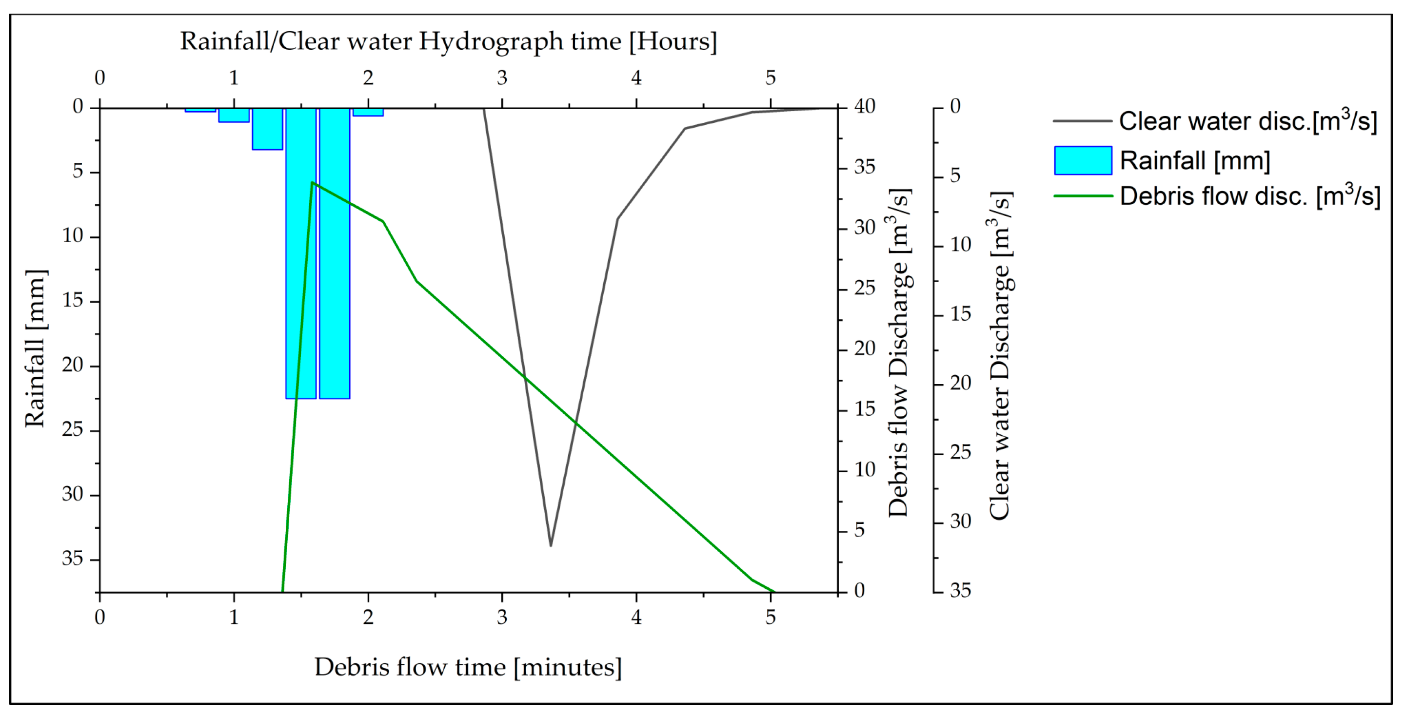
Based on the SCS analysis, the discharge of the Rio Sonno was estimated, yielding a peak flow to be 33 m³/s (Figure 3), which is consistent with the intensity and the duration of the rainfall event that triggered it. Subsequently, the debris flow discharge was calculated using the formula of Gregoretti and Della Fontana [3]. The resulting peak discharge is comparable to the maximum clear-water flow, and the duration of the debris flow hydrograph is consistent with that of typical debris flow events.

Two sets of simulations were analyzed separately: (1) river flow conditions based exclusively on the recorded Liri River discharge, and (2) the combined river–debris flow scenario. In the latter case, the debris flow was simulated by including the inflow hydrograph derived for the Rio Sonno tributary. Results are discussed in terms of water surface elevation, flow velocity, and the sediment total load capacity and concentration.

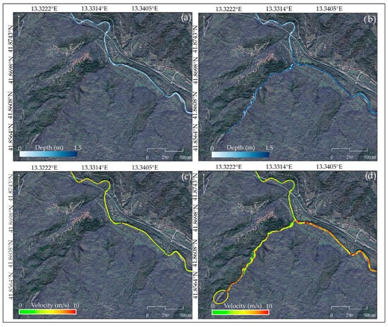
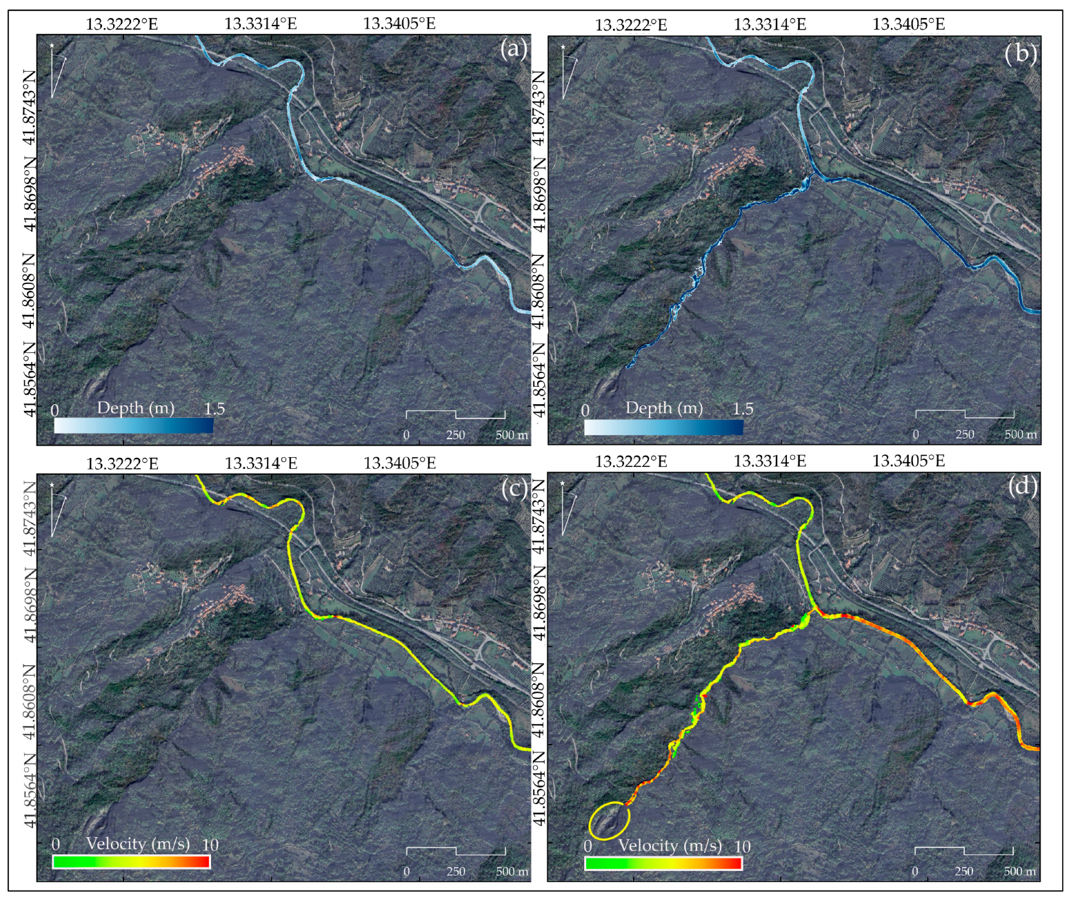
In conditions where only the river was considered, the simulated peak discharge at the analysis section of the Liri River produced a maximum water depth of 1.0 m., with average flow velocities ranging from 3 to 7 m/s (Figure 4a,b). In the combined scenario, the maximum water depth increased to 1.5 m along the Rio Sonno channel. Velocities also increased significantly, reaching up to 10 m/s in the source area and in the right-bank section of the Liri River. This was influenced by backwater effects and the sediment/discharge flux from the Rio Sonno (Figure 4c,d).

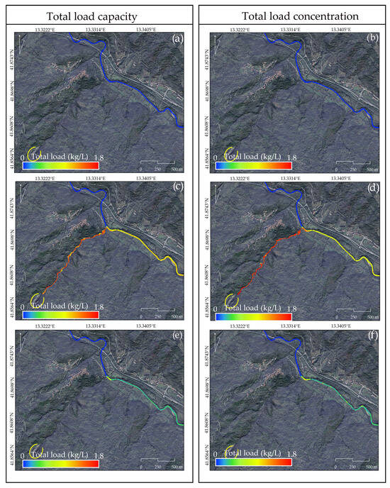
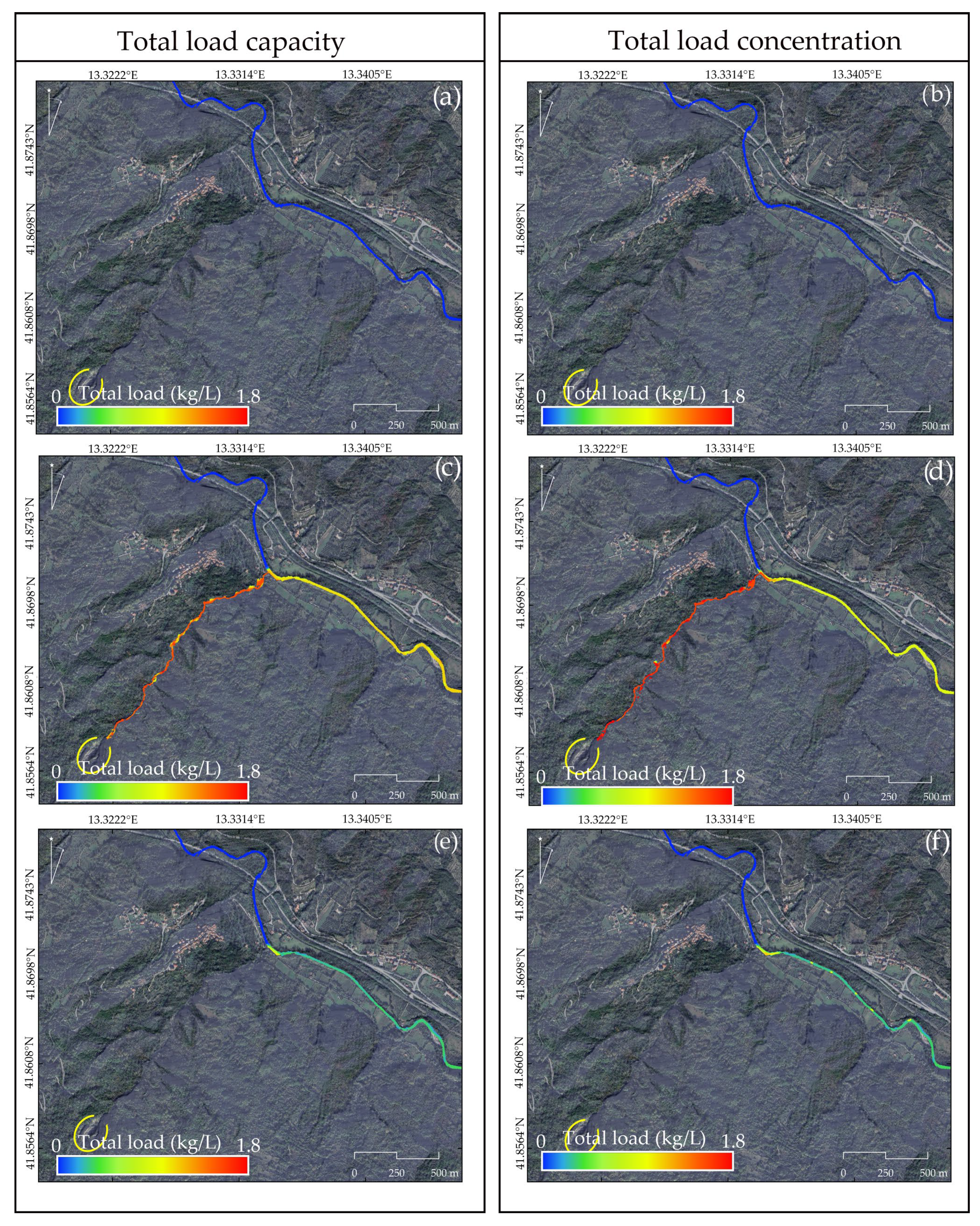
Figure 5 shows the temporal evolution of sediment transport, expressed in terms of total load capacity and total load concentration. Before the debris flow event (Figure 5a,b), sediment transport remained relatively low, with localized increases near the confluence. During the debris flow event (Figure 5c,d), pronounced peaks in both capacity and concentration were observed with maximum values of around 1.8 kg/L that is reasonable in the debris flow scenario [64]. In this case, the total load concentration is clearly lower than the total load capacity. This indicates that sediment is being deposited at the interface with the Liri River. The sediment transport is affecting the entire right-bank section of the Liri River. Considering Figure 5, before the debris flow event, sediment concentration reached a maximum of around 0.5 kg/L with flow velocity near 5 m/s in the source area. During the event, concentration peaked at 1.6 kg/L and velocity at 9 m/s, corresponding to increases of approximately 95% and 45%, respectively. After the event, both values gradually decreased to 0.9 kg/L and 5 m/s, reflecting rapid sediment deposit and recovery of clear-water conditions. This behaviour is consistent with the material that was initially scoured from the Rio Sonno channel being progressively absorbed into the main river flow. After the event (Figure 5e,f), sediment transport gradually decreased, indicating a return to clear-water conditions following the maximum sediment input associated with the debris flow.

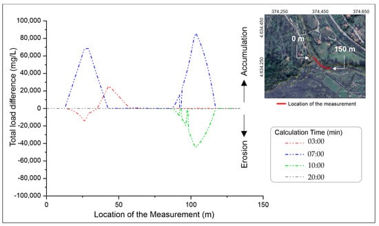
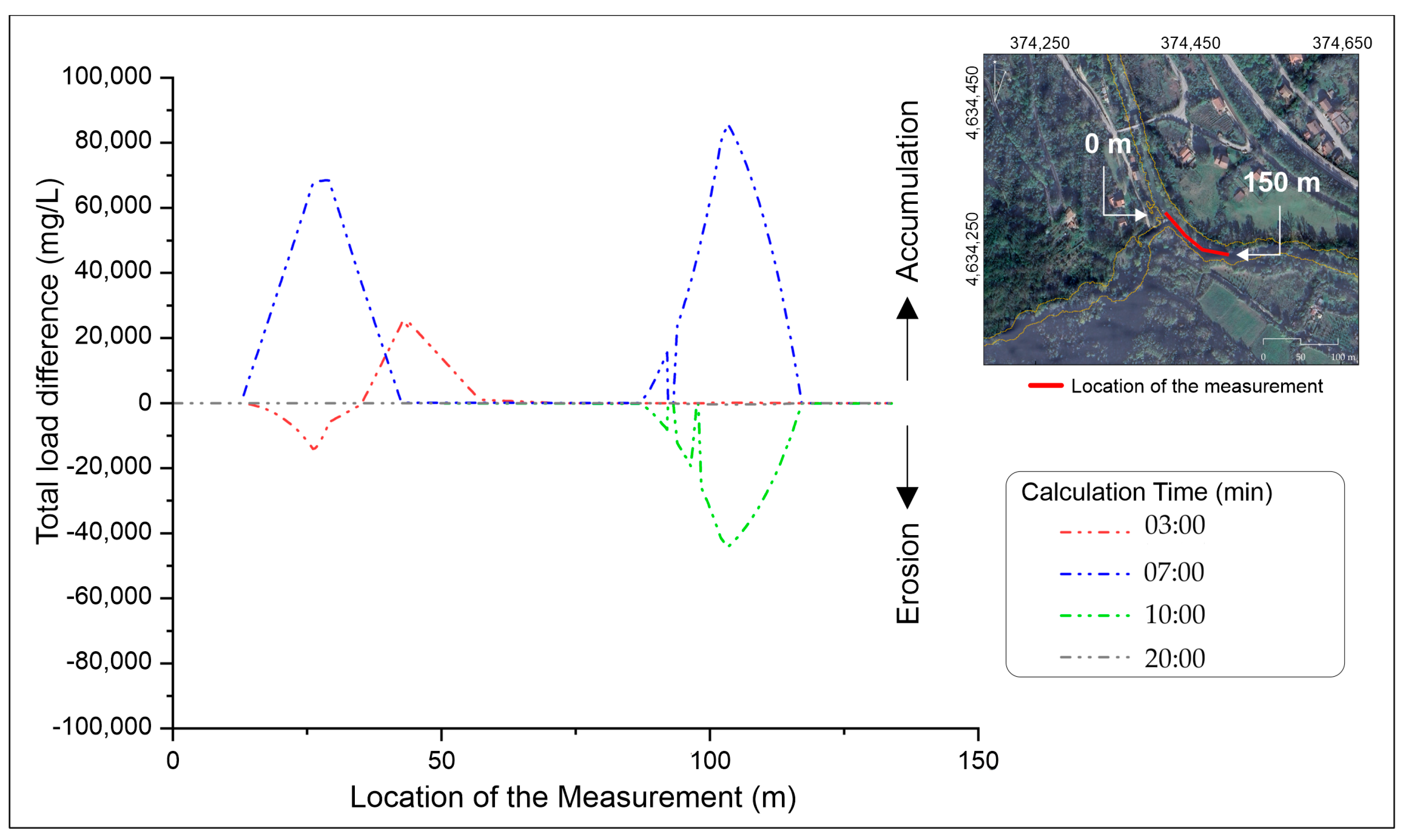
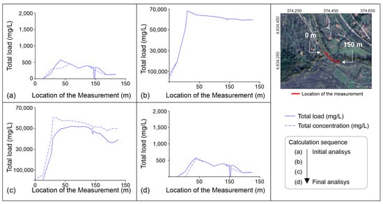
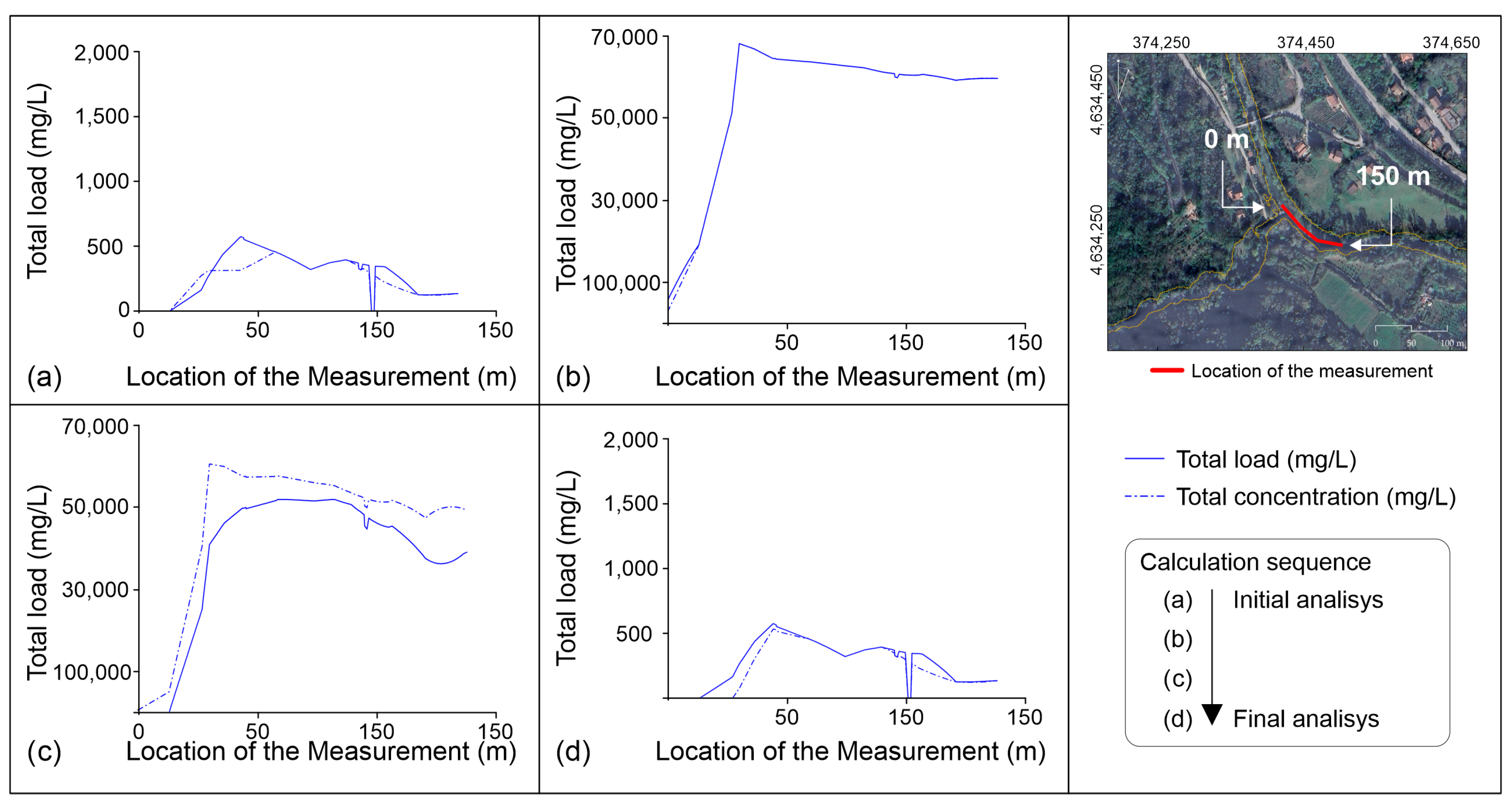
A cross-section at the confluence was analysed to determine the relationship between total load capacity and total load concentration (Figure 6). It was observed that, in the initial stage of granular flow input into the Liri River, the system maintained equilibrium between sediment transport and its transport capacity [65,66]. However, as the debris flow continued, the balance was shifted in favour of deposition. Subsequently, the system gradually returned to equilibrium as sediment input decreased and clear-water conditions resumed. Following the sediment input, the river system experiences a rapid imbalance between transport capacity and the amount of material supplied. This results in an immediate peak within the first few meters downstream. This is attributed to an increase in local turbulence and shear stress. During the debris flow, the concentration difference peaked at 20,000 mg/L, 3 min after the impact. The main deposition phase occurred about 7 min after the sediment pulse, with an additional increase of 80,000 mg/L, and near-equilibrium conditions were restored after roughly 20 min, reflecting the temporal adjustment of sediment transport and deposition. Over the next ~50 m, an adjustment phase occurs during which some of the material is temporarily deposited and the flow becomes progressively diluted. This results in a reduction in the capacity/input ratio compared to the initial value. The main deposition phase takes place approximately 7 min. after the arrival of the sediment pulse [52,53]. The restoration of the near-equilibrium conditions requires longer timescales, on the order of ~20 min.

Figure 7 shows the temporal evolution of the difference between the total load capacity and the total load concentration at the confluence between the Rio Sonno and the Liri River. Initially, the difference remains close to zero, suggesting that sediment transport is in equilibrium as the granular flow enters the main river. An intensification of the debris flow results in a negative difference, highlighting a phase dominated by sediment deposition at the confluence. Subsequently, the system gradually returned to equilibrium as the input of sediment decreased and clear-water conditions resumed. These dynamics highlight the transient nature of sediment fluxes during debris flow events and their significant impact on the channel’s sediment budget.

4.2. Dam-Break Results

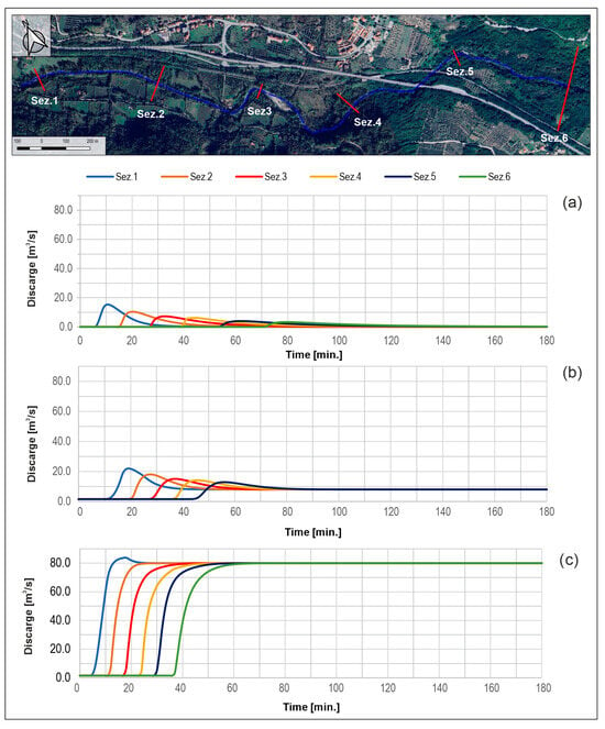
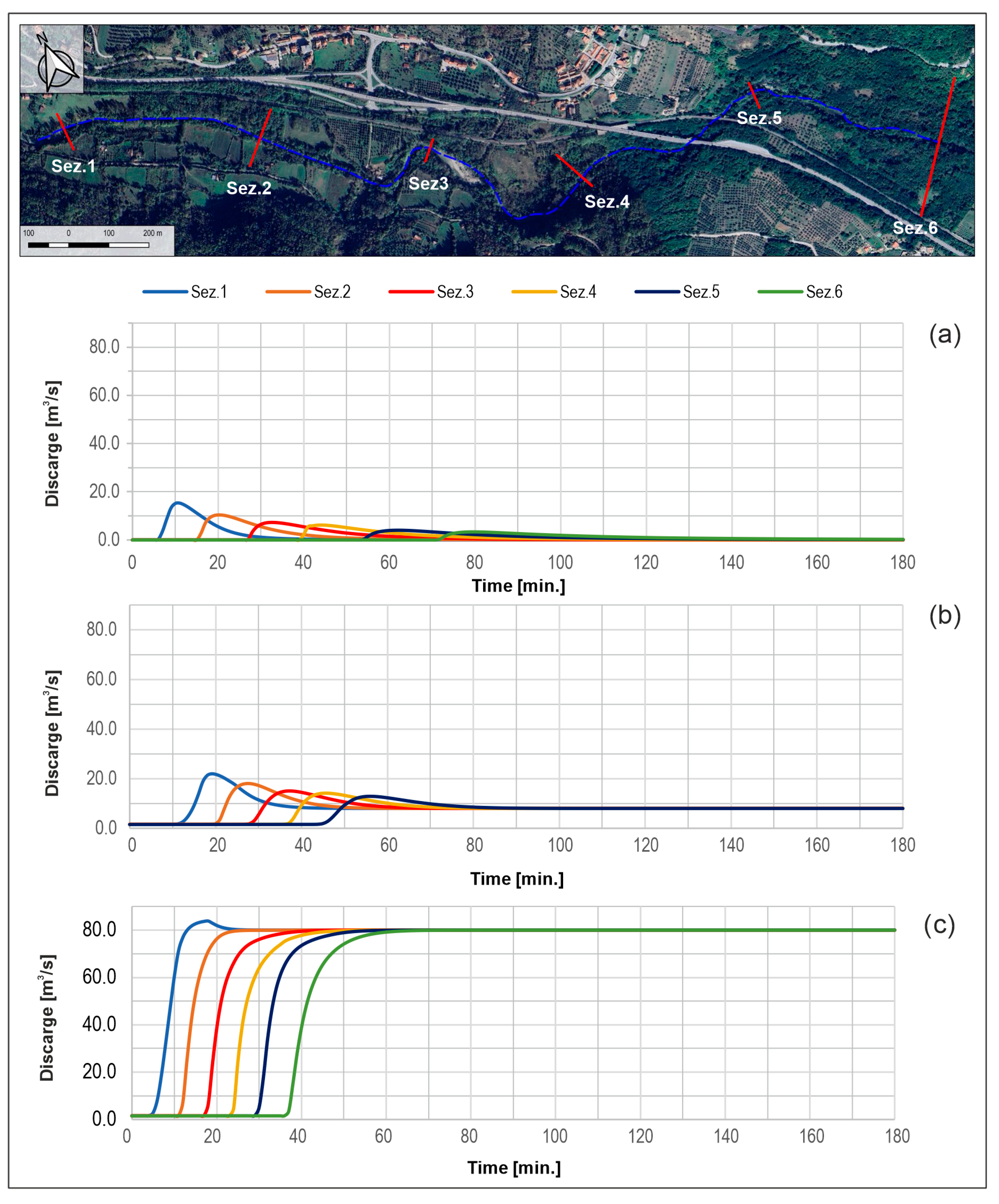
This section presents the key findings of the analyses conducted to simulate the breach of the natural dam formed on the Liri River after the debris flow along the Rio Sonno. Figure 8 shows the results of the three conditions that were simulated.

Scenario 1 (Figure 8a), characterized by the reservoir only, shows a significant attenuation of the peak discharges along the river reach is observed, with values decreasing from approximately 15.3 m³/s to 3.3 m³/s. At the same time, the time to peak progressively increases, ranging from 11 to 80 min. This behavior indicates a marked slowdown in the propagation of the flood wave along the reach. The average propagation velocity along the entire stretch, calculated between successive 500-m. intervals, shows a progressive decrease downstream, with intermediate values ranging between 0.46 and 0.93 m/s, and an overall average velocity of approximately 0.65 m/s. These results clearly demonstrate the reservoir’s damping effect, which reduces the wave energy and delays its propagation. Scenario 2 (Figure 8b), characterized by a discharge release of around 8 m³/s, shows that the peak flows are higher than in Scenario 1, ranging from 22 to 12 m³/s. However, attenuation is still evident along the river reach. In this case, the wave propagation velocity is more uniform along the stretch, with only a slight decrease in the downstream sections. With an average velocity of about 0.87 m/s, the flood wave appears to retain most of its initial energy during transit, although it does slow down slightly downstream. Scenario 3 (Figure 8c), characterized by a discharge of 80 m³/s, shows a different behaviour compared to the other simulations. The hydrographs quickly approach an asymptotic value, reaching 90% of the inflow discharge. The times to reach this value indicate a faster wave propagation than in the lower-flow scenarios. The velocity, calculated along successive intervals, varies between 0.83 and 1.67 m/s, with an overall average of approximately 1.18 m/s. This increase in propagation velocity show that the wave has a higher energy. This maintains high discharges along the river reach and reduces the reservoir’s damping effect.

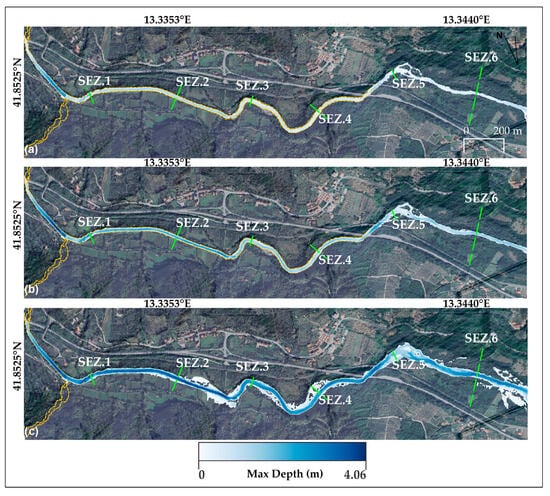
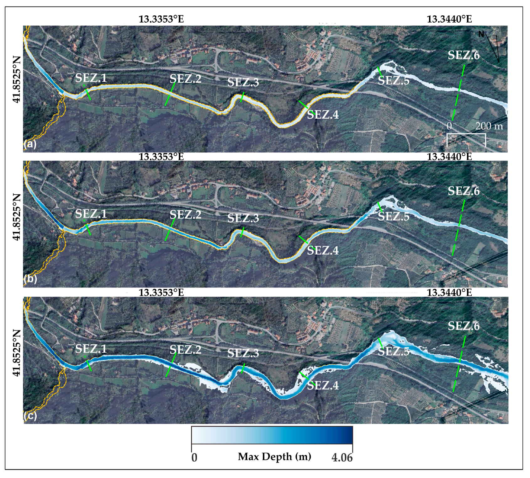
The spatial distribution of water flow height (Figure 9) shows a clear increase with the magnitude of the inflow discharge. In Scenario 1, the water levels remain largely confined within the main channel, indicating limited inundation and a strong damping effect of the reservoir. In Scenario 2, higher inflows lead to a moderate rise in water surface elevation, with occasional overflow near the downstream sections. Scenario 3 displays the most pronounced response, with markedly higher water levels and extensive inundation along the floodplain. These results confirm that the hydraulic response of the system is strongly influenced by discharge magnitude, as larger inflows produce higher water depths and more significant overbank flooding.

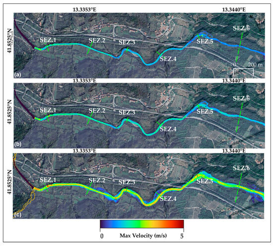
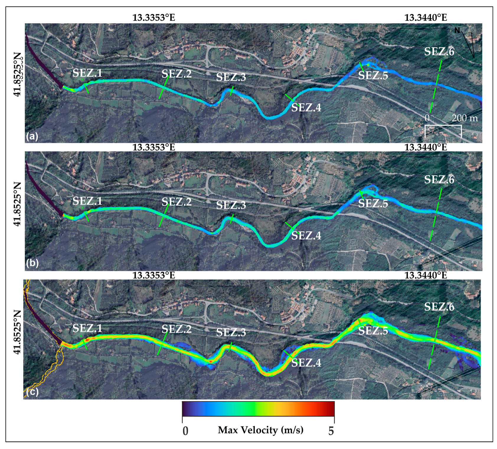
The spatial patterns of flow velocity follow similar trends to those observed in water height patterns (Figure 10). In Scenario 1 (Figure 10a), velocities are generally low throughout the reach, reflecting the strong attenuation and energy dissipation imposed by the reservoir. In Scenario 2 (Figure 10b), the flow accelerates moderately, maintaining relatively uniform values along the channel. Scenario 3 (Figure 10c) shows the highest velocities, particularly in the downstream sections, where the wave energy remains high and the damping effects are minimal. Overall, the increase in velocity as a function of discharge magnitude highlights the direct relationship between flow energy and the system’s hydraulic behavior.

In all scenarios, it is important to note that the modelling accounted for the time taken to fill the reservoir. The reported velocities therefore represent the actual propagation of the flood wave downstream, providing a realistic measure of the dynamics of the hydraulic system’s dynamics. The comparison of the results highlights a clear relationship between the magnitude of the inflow and both the peak attenuation and the propagation velocity. Scenario 1, as the lowest inflow, shows the strongest damping effect and the greatest increase in time to peak. It also has the lowest average propagation velocity. Scenario 2 presents intermediate characteristics, featuring higher peaks, moderate attenuation, and a relatively uniform propagation velocity. Finally, in scenario 3, the highest inflow, displays minimal attenuation, faster wave propagation, and higher average velocities. This indicates that the energy of the flood wave dominates over the reservoir’s damping effects. Overall, these results demonstrate that both the magnitude of the inflow and the presence of the reservoir both significantly influence the timing and the velocity of flood wave propagation. Comparing them provides insight into how flood waves of different magnitudes interact with hydraulic structures, which is crucial for accurately assessing and managing flood risk

5. Discussion

This study employs the SCS-CN method (Soil Conservation Service Curve Number) as a straightforward approach to transform recorded rainfall into a runoff hydrograph for the Rio Sonno basin. However, the procedure’s assumptions—constant Curve Number, homogeneous antecedent moisture conditions, and empirical λ-factor—introduce uncertainty in peak discharge estimates. Sensitivity tests indicate a variation of ±15% in Q_p for reasonable CN adjustments. This highlighting the importance of using field-calibrated CN values when applying SCS-CN method to small, steep tributary catchments [67]. Under river-only conditions, the model produced a maximum depth of 1.0 m and velocities up to 7 m/s. When the debris flow hydrograph was imposed, depths rose to 1.5 m and velocities briefly reached 10 m/s near the confluence. The backwater effect and the increase in the energy grade line probably increased the shear stress on the riverbanks, raising local scour potential and the flood risk. This dynamic suggests that standard flood-only hazard maps may significantly underestimate water surface elevations and flow forces when tributaries carrying debris are active [68]. A temporal analysis of the total load capacity versus concentration revealed an initial equilibrium phase during the early stage of debris entrainment. This was followed by a deposition dominated period as the debris wave crest reached the main channel. Maximum deposition at the interface corresponded to significant negative differences (capacity > concentration), which confirms the role of limited sediment supply at peak flow. The return toward equilibrium following the debris flow highlights the river’s self-cleansing capacity when clear-water conditions resume. Such transient deposition–remobilization cycles are essential for estimating sediment budgets and changes in channel conveyance [69,70].

To validate our results of hydraulic and sediment transport, we used a super-elevation formula to estimate the velocity of the debris flow along the channel and then compared these with the predictions of the model. Field observations, derived from drone imagery capturing inundation extents and flow heights, were also used to benchmark water surface elevations. Both velocity and depth data showed good agreement with simulated values. Furthermore, our observed peak velocities and deposition patterns align with those reported by [58], reinforcing the model’s capability to reproduce first-order debris flow behavior in similar Alpine tributary settings [71]. The accuracy of the results may be affected by several approximations, including the rheological model chosen. The simplified Bingham approach in Debris-Lib neglects yield-stress variability and particle interactions, which may result in an underestimation of peak shear stresses and in the sediment properties. Other, spatial heterogeneity within the source area may cause local transport deviations. Our results are aligned with Gregoretti and Della Fontana [3], who documented brief but intense deposition pulses in debris-affected channels. Similarly, as reported in different studies [57,72], the sediment waves in small Alpine tributaries often produce short-lived backwater zones and localised aggradation at confluences [3,68,73,74,75,76]. This study does more than just observe the impact of a debris event; it also explores how the basic flow characteristics of the Liri River modify the dynamics of such an event. Two key processes are highlighted in particular:

• Attenuation: The increased flow of the Liri River has a diluting effect. When a sedimentary pulse loaded with debris enters the river, the existing water disperses the sediment, thereby reducing its impact and concentration.
• Propagation: The Liri’s constant current not only attenuates the pulse but helps it to move downstream more gradually and under great control. This transport mechanism prevents the accumulation of large amounts of debris in one area by distributing it over a wider zone.

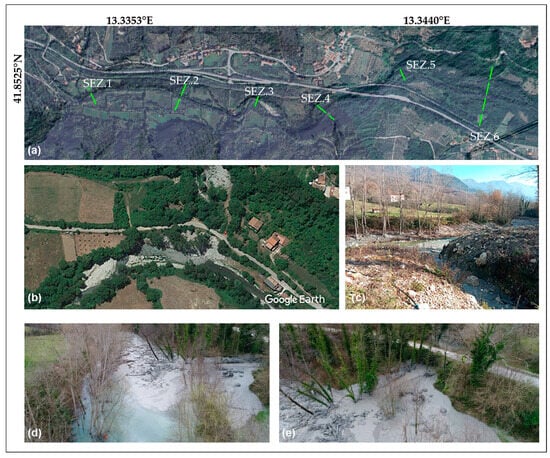
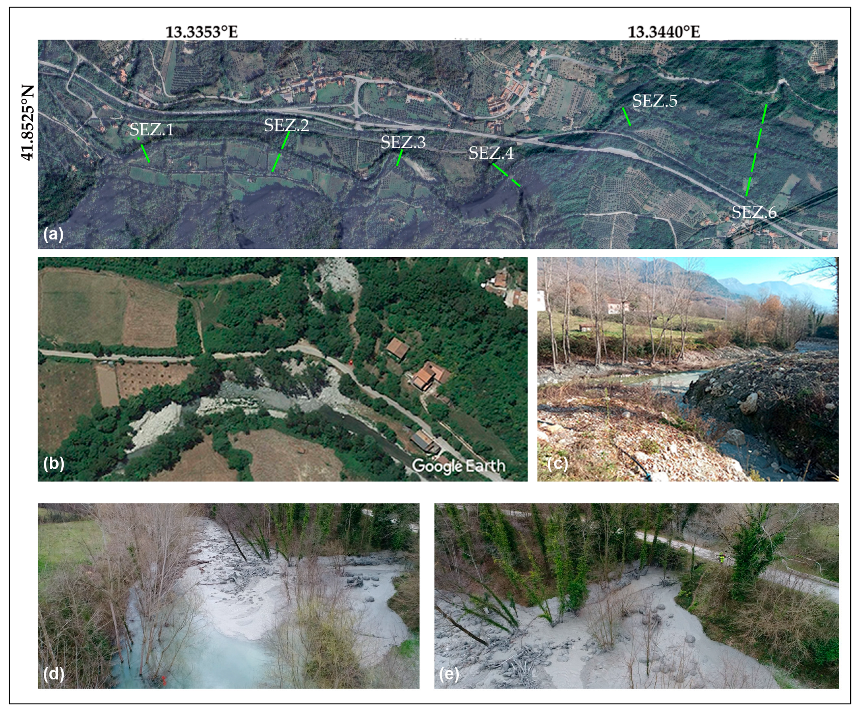
The Liri river system restores clear water conditions more gradually and rapidly than a system purely dominated by debris flow. In other words, the Liri manages the sedimentary pulse by reducing the duration of the negative impact on water quality and, consequently, on the present ecosystems. Figure 11 illustrates the observed data used for comparison with the simulation results. The field data show good agreement between the modelled water depths and velocities and those derived from field surveys and drone observations. The close correspondence between the two datasets confirms the model’s capability to reproduce the main hydraulic features of the event, starting from the Liri River damming and including the spatial extent of inundation and the peak flow dynamics. Minor discrepancies can be attributed to local topographic irregularities and temporal variations during data acquisition; overall, however, the results validate the reliability of the modelling approach.

The results of the previously presented scenarios can be further interpreted in the context of dam-break dynamics and flood wave propagation. While the scenarios focused on clear water discharges, the presence of a sudden inflow, such as a debris-laden pulse, can temporarily amplify peak depths and velocities, particularly near confluences or constricted channel sections. This behavior is consistent with the trends observed across the scenarios: higher inflows produce faster, less attenuated waves, whereas lower flows are progressively slowed and damped along the reach.

The flow of the river acts to both propagate the flood wave downstream and to attenuate its peak. This reduces the risk of localized inundation. Figure 11b–d clearly shows the close correspondence between the simulation results and the field observations. The matching patterns of water depth and flow velocity demonstrate that the model accurately reproduces the observed hydraulic behavior, including the extent of inundation and the spatial distribution of peak flow. These consistencies further confirm the robustness of the numerical approach and the reliability of the calibration based on field data. Only minor sediment-related effects, such as brief deposition or local scouring near the channel interface, were observed, confirming that the primary control on the water surface elevations and velocities is the dynamics of the flood wave itself. These insights highlight the importance of accurately modelling both the magnitude and timing of inflows when assessing dam-break scenarios.

6. Conclusions

The integrated hydraulic and sediment transport analyses provide a comprehensive understanding of how inflow magnitude, sediment load, and channel conditions jointly control the hydrodynamic response of the Liri River system. Although the SCS-CN method was effective in translating rainfall inputs into runoff hydrographs, the sensitivity of peak discharge to variations in the Curve Number highlights the need for site-specific calibration in steep Alpine catchments. The scenario simulations demonstrated that flow attenuation and propagation are strongly governed by the magnitude of the inflow and the damping effect of the reservoir. Low inflows promote pronounced wave attenuation and delayed peaks, whereas high inflows generate faster, more energetic waves with minimal damping. When debris-laden inflows are introduced, both depths and velocities increase significantly, especially near the confluence, amplifying local scour potential and short-term flood hazard. Sediment transport analysis revealed a cyclical pattern of deposition and remobilization, reflecting the system’s ability to recover and re-establish equilibrium once clear water conditions return. This self-cleansing behavior, combined with the Liri’s continuous base flow, enables the river to disperse sediment pulses efficiently, limiting long-term morphological instability. Model–observation agreement, supported by field and drone data, validates the numerical approach and its capacity to reproduce key hydraulic and morpho-dynamic processes. However, uncertainties remain due to rheological simplifications and spatial heterogeneity within the source areas. These limitations highlight the importance of coupling physically based rheological models with detailed field measurements to refine predictions of debris flow behavior. Overall, the study emphasizes that the interaction between flood waves and debris inflows cannot be neglected in hazard assessment. Accurate representation of inflow magnitude, timing, and sediment load is crucial for realistic simulation of dam-break and debris-flood scenarios. By capturing both attenuation and propagation mechanisms, the modelling framework adopted here provides valuable insights for flood risk management and sediment dynamics in complex Alpine catchment systems. Beyond its application to the Liri River case, this work demonstrates the value of integrated modelling approaches that combine hydraulic and sediment dynamics to provide a comprehensive analysis of river systems. Such frameworks support water resource management by improving the prediction of sediment budgets and flood responses under varying environmental conditions. Future research should improve debris-flow modelling and account for spatial variability in source areas, with particular focus on climate-change-driven extremes such as intense rainfall and altered snowmelt. Integrating long-term field and remote sensing data will refine predictions of flood-wave and sediment dynamics, supporting resilient river management in different environments. They also contribute to ecosystem protection by identifying zones of morphological sensitivity and guiding nature-based mitigation measures. Ultimately, this integrated approach strengthens georisk reduction strategies, thereby enhancing the resilience of mountain catchments to cascading hydrogeomorphic hazards.

References

- Hungr, O. Momentum Transfer and Friction in the Debris of Rock Avalanches: Discussion. Can. Geotech. J. 2011, 27, 697. [Google Scholar] [CrossRef] [Scilit]
- Iverson, R.M.; Reid, M.E.; LaHusen, R.G. Debris-Flow Mobilization from Landslides. Annu. Rev. Earth Planet. Sci. 1997, 25, 85–138. [Google Scholar] [CrossRef] [Scilit]
- Gregoretti, C.; Fontana, G.D. The Triggering of Debris Flow Due to Channel-Bed Failure in Some Alpine Headwater Basins of the Dolomites: Analyses of Critical Runoff. Hydrol. Process. 2008, 22, 2248–2263. [Google Scholar] [CrossRef] [Scilit]
- Lee, C.F.; Dai, F.C. The 1786 Dadu River Landslide Dam, Sichuan, China; Springer: Berlin/Heidelberg, Germany, 2011; pp. 369–388. [Google Scholar] [CrossRef] [Scilit]
- Choi, C.E.; Cui, Y.; Au, K.Y.K.; Liu, H.; Wang, J.; Liu, D.; Wang, H. Case Study: Effects of a Partial-Debris Dam on Riverbank Erosion in the Parlung Tsangpo River, China. Water 2018, 10, 250. [Google Scholar] [CrossRef] [Scilit]
- Chen, H.; Ruan, H.; Chen, J.; Li, X.; Yu, Y. Review of Investigations on Hazard Chains Triggered by River-Blocking Debris Flows and Dam-Break Floods. Front. Earth Sci. 2022, 10, 830044. [Google Scholar] [CrossRef] [Scilit]
- Fan, X.; Yang, F.; Siva Subramanian, S.; Xu, Q.; Feng, Z.; Mavrouli, O.; Peng, M.; Ouyang, C.; Jansen, J.D.; Huang, R. Prediction of a Multi-Hazard Chain by an Integrated Numerical Simulation Approach: The Baige Landslide, Jinsha River, China. Landslides 2019, 17, 147–164. [Google Scholar] [CrossRef] [Scilit]
- Prancevic, J.P.; Lamb, M.P.; Fuller, B.M. Incipient Sediment Motion across the River to Debris-Flow Transition. Geology 2014, 42, 191–194. [Google Scholar] [CrossRef] [Scilit]
- Shu, A.; Wang, L.; Zhu, F.; Zhu, J.; Pi, C.; Zhang, Z.; Huarez, C. Hydrodynamic Process of Partial and En Masse Dam Failure Induced Debris Flows. Front. Environ. Sci. 2022, 10, 905499. [Google Scholar] [CrossRef] [Scilit]
- Jhong, B.C.; Huang, J.; Tung, C.P. Spatial Assessment of Climate Risk for Investigating Climate Adaptation Strategies by Evaluating Spatial-Temporal Variability of Extreme Precipitation. Water Resour. Manag. 2019, 33, 3377–3400. [Google Scholar] [CrossRef] [Scilit]
- Lin, M.-L.; Lin, S.-C.; Lin, Y.-C. Review of Landslide Occurrence and Climate Change in Taiwan. In Slope Safety Preparedness for Impact of Climate Change; CRC Press: Boca Raton, FL, USA, 2017; pp. 409–436. [Google Scholar] [CrossRef] [Scilit]
- Zhou, X.; Du, X.; Zhou, J.; Yang, Z.; Jiang, T.; Chen, W. Draining the Successive Baige Barrier Lakes, China: Insight into the Emergency Response. Nat. Hazards Rev. 2024, 25, 05024006. [Google Scholar] [CrossRef] [Scilit]
- Pudasaini, S.P.; Fischer, J.T. A Mechanical Erosion Model for Two-Phase Mass Flows. Int. J. Multiph. Flow 2020, 132, 103416. [Google Scholar] [CrossRef] [Scilit]
- Gibson, S.; Moura, L.Z.; Ackerman, C.; Ortman, N.; Amorim, R.; Floyd, I.; Eom, M.; Creech, C.; Sánchez, A. Prototype Scale Evaluation of Non-Newtonian Algorithms in HEC-RAS: Mud and Debris Flow Case Studies of Santa Barbara and Brumadinho. Geosciences 2022, 12, 134. [Google Scholar] [CrossRef] [Scilit]
- Xia, C.; Tian, H. A Quasi-Single-Phase Model for Debris Flows Incorporating Non-Newtonian Fluid Behavior. Water 2022, 14, 1369. [Google Scholar] [CrossRef] [Scilit]
- Tiranti, D.; Crema, S.; Cavalli, M.; Deangeli, C. An Integrated Study to Evaluate Debris Flow Hazard in Alpine Environment. Front. Earth Sci. 2018, 6, 356666. [Google Scholar] [CrossRef] [Scilit]
- Morgenstern, R.; Massey, C.; Rosser, B.; Archibald, G. Landslide Dam Hazards: Assessing Their Formation, Failure Modes, Longevity and Downstream Impacts. In Understanding and Reducing Landslide Disaster Risk; Springer: Berlin/Heidelberg, Germany, 2021; pp. 117–123. [Google Scholar] [CrossRef] [Scilit]
- Liu, W.; Yan, S.; He, S. A Simple Method to Evaluate the Performance of an Intercept Dam for Debris-Flow Mitigation. Eng. Geol. 2020, 276, 105771. [Google Scholar] [CrossRef] [Scilit]
- Chen, K.T.; Lin, C.H.; Chen, X.Q.; Hu, G.S.; Guo, X.J.; Shieh, C.L. An Assessment Method for Debris Flow Dam Formation in Taiwan. Earth Sci. Res. J. 2018, 22, 37–43. [Google Scholar] [CrossRef] [Scilit]
- Gibson, S.; Floyd, I.; Sánchez, A.; Heath, R. Comparing Single-Phase, Non-Newtonian Approaches with Experimental Results: Validating Flume-Scale Mud and Debris Flow in HEC-RAS. Earth Surf. Process. Landf. 2021, 46, 540–553. [Google Scholar] [CrossRef] [Scilit]
- De Vita, P.; Piscopo, V. Influences of Hydrological and Hydrogeological Conditions on Debris Flows in Peri-Vesuvian Hillslopes. Nat. Hazards Earth Syst. Sci. 2002, 2, 27–35. [Google Scholar] [CrossRef] [Scilit]
- Del Soldato, M.; Tomás, R.; Festa, D.; Floyd, I.E.; Sánchez, A.; Gibson, S.; Savant, G. A Modular, Model, Library Framework (DebrisLib) for Non-Newtonian Geophysical Flows. Geosciences 2025, 15, 240. [Google Scholar] [CrossRef] [Scilit]
- Mangifesta, M.; Aringoli, D.; Pambianchi, G.; Giannini, L.M.; Scalella, G.; Sciarra, N. A Methodologic Approach to Study Large and Complex Landslides: An Application in Central Apennines. Geosciences 2024, 14, 272. [Google Scholar] [CrossRef] [Scilit]
- Collettini, C.; Barchi, M.R. A Low-Angle Normal Fault in the Umbria Region (Central Italy): A Mechanical Model for the Related Microseismicity. Tectonophysics 2002, 359, 97–115. [Google Scholar] [CrossRef] [Scilit]
- Calamita, F.; Centamore, E.; Deiana, G.; Ridolfi, M. Caratterizzazione Geologico-Strutturale Dell’area Marchigiano-Abruzzese Esterna (Appennino Centrale). Studi Geol. Camerti. Nuova Ser. 2023, 1, 171–182. [Google Scholar]
- Zito, C.; Mangifesta, M.; Francioni, M.; Guerriero, L.; Di Martire, D.; Calcaterra, D.; Cencetti, C.; Pasculli, A.; Sciarra, N. Numerical Modelling of Rock Fragmentation in Landslide Propagation: A Test Case. Geosciences 2025, 15, 354. [Google Scholar] [CrossRef] [Scilit]
- Lloyd, J.; Christie, N.; Lock, G. From the Mountain to the Plain: Landscape Evolution in the Abruzzo. An Interim Report on the Sangro Valley Project (1994–5). Pap. Br. Sch. Rome 1997, 65, 1–57. [Google Scholar] [CrossRef] [Scilit]
- Martini, I.P.; Wightman, E.M. Geomorphology and Ancient Settlements of the Southern Flank of MT. Cairo, Lower Liri Valley, Italy. Geoarchaeology 1987, 2, 131–147. [Google Scholar] [CrossRef] [Scilit]
- Paglia, G.; Carabella, C.; Epifani, C.; Esposito, G.; Fazzini, M.; Mancinelli, V.; Miccadei, E. Landslide Hazard in the Abruzzo Area (Central Italy): Case Studies of Different Types of Landslides in Different Environments and Morphostructural Domains. In Proceedings of the EGU General Assembly, Online, 4–8 May 2020. [Google Scholar] [CrossRef] [Scilit]
- Curci, G.; Guijarro, J.A.; Di Antonio, L.; Di Bacco, M.; Di Lena, B.; Scorzini, A.R. Building a Local Climate Reference Dataset: Application to the Abruzzo Region (Central Italy), 1930–2019. Int. J. Climatol. 2021, 41, 4414–4436. [Google Scholar] [CrossRef] [Scilit]
- Cosentino, D.; Cipollari, P. The Messinian Central Apennines. Rend. Online Soc. Geol. Ital. 2012, 23, 45–51. [Google Scholar]
- Miccadei, E.; Piacentini, T.; Buccolini, M. Long-Term Geomorphological Evolution in the Abruzzo Area, Central Italy: Twenty Years of Research. Geol. Carpathica 2017, 68, 19–28. [Google Scholar] [CrossRef] [Scilit]
- Parotto, M. Stratigrafy and Tectonics of the Eastern Simbruini and Western Marsica Ranges (Central Apennines—Italy). Atti. Accad. Naz. Lincei Mem. 1971, 8, 93–170. [Google Scholar]
- Ogniben, L.; Parotto, M.; Praturlon, A. (Eds.) Structural Model of Italy; Paper Covers in Slip Case (1975) No. 90.|Acanthophyllum Books; Consiglio Nazionale Delle Ricerche: Rome, Italy, 1975; Available online: https://www.abebooks.com/Structural-model-Italy-Ogniben-Parotto-Praturlon/31517628636/bd (accessed on 12 May 2025).
- Calamita, F.; Deiana, G. The Arcuate Shape of the Umbria-Marche-Sabina Apennines (Central Italy). Tectonophysics 1988, 146, 139–147. [Google Scholar] [CrossRef] [Scilit]
- Zito, C.; Mangifesta, M.; Francioni, M.; Guerriero, L.; Di Martire, D.; Calcaterra, D.; Sciarra, N. Cascading Landslide: Kinematic and Finite Element Method Analysis through Remote Sensing Techniques. Remote Sens. 2024, 16, 3423. [Google Scholar] [CrossRef] [Scilit]
- Zito, C.; Mangifesta, M.; Francioni, M.; Guerriero, L.; Martire, D.D.; Calcaterra, D.; Pasculli, A.; Sciarra, N. Cascading Landslides at Morino-Rendinara, L’Aquila, Central Italy: Numerical Modelling of Slope-Scale Prospective Debris Flow Propagation. Ital. J. Eng. Geol. Environ. 2024, 285–293. [Google Scholar] [CrossRef]
- George, D.L.; Iverson, R.M. A Depth-Averaged Debris-Flow Model That Includes the Effects of Evolving Dilatancy. II. Numerical Predictions and Experimental Tests. Proc. R. Soc. A Math. Phys. Eng. Sci. 2014, 470, 20130820. [Google Scholar] [CrossRef] [Scilit]
- Armanini, A.; Gregoretti, C. Triggering of Debris-Flow by Overland Flow: A Comparison between Theoretical and Experimental Results. In Proceedings of the Debris-Flow Hazards Mitigation: Mechanics, Prediction, and Assessment, Taipei, China, 16–18 August 2000; pp. 117–124. [Google Scholar]
- Tognacca, C.; Bezzolla, G.R.; Minor, H.-E. Threshold Criterion for Debris-Flow Initiation Due to Channel-Bed Failure. In Proceedings of the Debris-Flow Hazards Mitigation: Mechanics, Prediction, and Assessment, Taipei, China, 16–18 August 2000; pp. 89–97. [Google Scholar]
- Hjelmfelt, A.T. Investigation of Curve Number Procedure. J. Hydraul. Eng. 1991, 117, 725–737. [Google Scholar] [CrossRef] [Scilit]
- Mishra, S.K.; Singh, V.P. Soil Conservation Service Curve Number (SCS-CN) Methodology. Water Sci. Technol. Libr. 2003, 42, 355–362. [Google Scholar] [CrossRef] [Scilit]
- McCuen, R.H. Approach to Confidence Interval Estimation for Curve Numbers. J. Hydrol. Eng. 2002, 7, 43–48. [Google Scholar] [CrossRef] [Scilit]
- Moore, R.J.; Clarke, R.T. A Distribution Function Approach to Rainfall Runoff Modeling. Water Resour. Res. 1981, 17, 1367–1382. [Google Scholar] [CrossRef] [Scilit]
- Grove, M.; Harbor, J.; Engel, B. Composite vs. Distributed Curve Numbers: Effects on Estimates of Storm Runoff Depths. J. Am. Water Resour. Assoc. 1998, 34, 1015–1023. [Google Scholar] [CrossRef] [Scilit]
- Finnerty, B.D.; Smith, M.B.; Seo, D.J.; Koren, V.; Moglen, G.E. Space-Time Scale Sensitivity of the Sacramento Model to Radar-Gage Precipitation Inputs. J. Hydrol. 1997, 203, 21–38. [Google Scholar] [CrossRef] [Scilit]
- Bosznay, M. Generalization of SCS Curve Number Method. J. Irrig. Drain. Eng. 1989, 115, 139–144. [Google Scholar] [CrossRef] [Scilit]
- Mockus, V. Estimation of Direct Runoff from Storm Rainfall. In National Engineering Handbook; US Department of Agriculture: Washington, DC, USA, 1972; Volume 10, p. 22. [Google Scholar]
- Pasculli, A.; Zito, C.; Mangifesta, M.; Sciarra, N. Back Analysis of a Real Debris Flow, the Morino-Rendinara Test Case (Italy), Using RAMMS Software. Land 2024, 13, 2078. [Google Scholar] [CrossRef] [Scilit]
- Pastor, M.; Merodo, J.A.F.; Quecedo, M.; Herreros, M.I.; González, E.; Mira, P. Modelling of Debris Flows and Flow Slides. Rev. Française Génie Civ. 2002, 6, 1213–1232. [Google Scholar] [CrossRef] [Scilit]
- Zanuttigh, B.; Lamberti, A. Analysis of Debris Wave Development with One-Dimensional Shallow-Water Equations. J. Hydraul. Eng. 2004, 130, 293–304. [Google Scholar] [CrossRef] [Scilit]
- Michaelides, K.; Martin, G.J. Sediment Transport by Runoff on Debris-Mantled Dryland Hillslopes. J. Geophys Res. Earth Surf. 2012, 117, 3014. [Google Scholar] [CrossRef] [Scilit]
- Damgaard, J.S.; Whitehouse, R.J.S.; Soulsby, R.L. Bed-Load Sediment Transport on Steep Longitudinal Slopes. J. Hydraul. Eng. 1997, 123, 1130–1138. [Google Scholar] [CrossRef] [Scilit]
- Rijn, L.C. van Sediment Transport, Part I: Bed Load Transport. J. Hydraul. Eng. 1984, 110, 1431–1456. [Google Scholar] [CrossRef] [Scilit]
- Zhang, Y.; Al-Hamdan, M.; Wren, D. Development of a Two-Dimensional Hybrid Sediment-Transport Model. Appl. Sci. 2023, 13, 4940. [Google Scholar] [CrossRef] [Scilit]
- Wang, Y.; Liang, Q.; Kesserwani, G.; Hall, J.W. A 2D Shallow Flow Model for Practical Dam-Break Simulations. J. Hydraul. Res. 2011, 49, 307–316. [Google Scholar] [CrossRef] [Scilit]
- Froehlich, D.C. Embankment Dam Breach Parameters and Their Uncertainties. J. Hydraul. Eng. 2008, 134, 1708–1721. [Google Scholar] [CrossRef] [Scilit]
- Froehlich, D.C. Peak Outflow from Breached Embankment Dam. J. Water Resour. Plan. Manag. 1995, 121, 90–97. [Google Scholar] [CrossRef] [Scilit]
- Abdulrazzaq, I.D.; Jalut, Q.H.; Abbas, J.M. Sensitivity Analysis for Dam Breach Parameters Using Different Approaches for Earth-Fill Dam. Diyala J. Eng. Sci. 2021, 14, 90–97. [Google Scholar] [CrossRef] [Scilit]
- Marinelli, F.; Buscarnera, G. A Generalized Backward Euler Algorithm for the Numerical Integration of a Viscous Breakage Model. Int. J. Numer. Anal. Meth. Geomech. 2019, 43, 3–29. [Google Scholar] [CrossRef] [Scilit]
- Diskin, B.; Thomas, J.L.; Rumsey, C.L.; Schwöppe, A. Grid Convergence for Turbulent Flows (Invited). In Proceedings of the 53rd AIAA Aerospace Sciences Meeting, Kissimmee, FL, USA, 5–9 January 2015. [Google Scholar]
- Muranushi, T. Paraiso: An Automated Tuning Framework for Explicit Solvers of Partial Differential Equations. Comput. Sci. Discov. 2012, 5, 015003. [Google Scholar] [CrossRef] [Scilit]
- Wharton, G.; Arnell, N.W.; Gregory, K.J.; Gurnell, A.M. River Discharge Estimated from Channel Dimensions. J. Hydrol. 1989, 106, 365–376. [Google Scholar] [CrossRef] [Scilit]
- Rickenmann, D. Hyperconcentrated Flow and Sediment Transport at Steep Slopes. J. Hydraul. Eng. 1991, 117, 1419–1439. [Google Scholar] [CrossRef] [Scilit]
- Cao, Z. Equilibrium Near-Bed Concentration of Suspended Sediment. J. Hydraul. Eng. 1999, 125, 1270–1278. [Google Scholar] [CrossRef] [Scilit]
- Waters, K.A.; Curran, J.C. Linking Bed Morphology Changes of Two Sediment Mixtures to Sediment Transport Predictions in Unsteady Flows. Water Resour. Res. 2015, 51, 2724–2741. [Google Scholar] [CrossRef] [Scilit]
- Silveira, L.; Charbonnier, F.; Genta, J.L. L’humidité Antérieure Des Sols Dans La Méthode “Curve Number”. Hydrol. Sci. J. 2000, 45, 3–12. [Google Scholar] [CrossRef] [Scilit]
- Pinter, N.; Thomas, R.; Wlosinski, J.H. Assessing Flood Hazard on Dynamic Rivers. Eos Trans. Am. Geophys. Union 2001, 82, 333–339. [Google Scholar] [CrossRef] [Scilit]
- Brunner, G.W.; Gibson, S. Sediment Transport Modeling in HEC RAS. World Water Congress 2005: Impacts of Global Climate Change. In Proceedings of the 2005 World Water and Environmental Resources Congress, Anchorage, AK, USA, 15–19 May 2005; p. 442. [Google Scholar] [CrossRef] [Scilit]
- Berghout, A.; Meddi, M. Sediment Transport Modelling in Wadi Chemora during Flood Flow Events. J. Water Land Dev. 2016, 31, 23–31. [Google Scholar] [CrossRef] [Scilit]
- Bertolo, P.; Wieczorek, G.F. Calibration of Numerical Models for Small Debris Flows in Yosemite Valley, California, USA. Nat. Hazards Earth Syst. Sci. 2005, 5, 993–1001. [Google Scholar] [CrossRef] [Scilit]
- Li, J.; Zhao, Y.; Bates, P.D.; Neal, J.C.; Tooth, S.; Hawker, L.; Maffei, C. Digital Elevation Models for Topographic Characterisation and Flood Flow Modelling along Low-Gradient, Terminal Dryland Rivers: A Comparison of Spaceborne Datasets for the Río Colorado, Bolivia. J. Hydrol. 2020, 591, 125617. [Google Scholar] [CrossRef] [Scilit]
- Parsons, J.D.; Whipple, K.X.; Simoni, A. Experimental Study of the Grain-Flow, Fluid-Mud Transition in Debris Flows. J. Geol. 2001, 109, 427–447. [Google Scholar]
- Mikoš, M.; Bezak, N. Debris Flow Modelling Using RAMMS Model in the Alpine Environment with Focus on the Model Parameters and Main Characteristics. Front. Earth Sci. 2021, 8, 605061. [Google Scholar] [CrossRef] [Scilit]
- Camporese, M.; Penna, D.; Borga, M.; Paniconi, C. A Field and Modeling Study of Nonlinear Storage-Discharge Dynamics for an Alpine Headwater Catchment. Water Resour. Res. 2014, 50, 806–822. [Google Scholar] [CrossRef] [Scilit]
- Panici, D.; Bennett, G. Modelling Landslide-Flood Interactions: An Example from Colorado. In Proceedings of the EGU General Assembly, Online, 19–30 April 2021. [Google Scholar] [CrossRef] [Scilit]
Disclaimer/Publisher’s Note: The statements, opinions and data contained in all publications are solely those of the individual author(s) and contributor(s) and not of MDPI and/or the editor(s). MDPI and/or the editor(s) disclaim responsibility for any injury to people or property resulting from any ideas, methods, instructions or products referred to in the content. |
© 2025 by the authors. Licensee MDPI, Basel, Switzerland. This article is an open access article distributed under the terms and conditions of the Creative Commons Attribution (CC BY) license (https://creativecommons.org/licenses/by/4.0/).