Comparison of Nature-Inspired Optimization Models and Robust Machine-Learning Approaches in Predicting the Sustainable Building Energy Consumption: Case of Multivariate Energy Performance Dataset

Abstract

Accurate prediction of building energy loads is essential for smart buildings and sustainable energy management. While machine learning (ML) approaches outperform traditional statistical models at capturing nonlinear relationships, most studies primarily optimize prediction accuracy, overlooking the importance of computational efficiency and feature compactness, which are critical in real-time, resource-constrained environments. This study aims to evaluate whether hybrid nature-inspired feature-selection techniques can enhance the accuracy and computational efficiency of ML-based building energy load prediction. Using the UCI Energy Efficiency dataset, eight ML models (LightGBM, CatBoost, XGBoost, Decision Tree, Random Forest, Extra Trees, Linear Regression, Support Vector Regression) were trained under feature subsets obtained from the Butterfly Optimization Algorithm (BOA), Grey Wolf Optimization Algorithm (GWO), and a hybrid BOA–GWO approach. Model performance was evaluated using three metrics (MAE, RMSE, and R²), along with training time, prediction time, and the number of selected features. The results show that gradient-boosting models consistently yield the highest accuracy, with CatBoost achieving an R² of 0.99 or higher. The proposed hybrid BOA–GWO method achieved competitive accuracy with fewer features and reduced training time, demonstrating its suitability for efficient ML deployment in smart building environments. Rather than proposing a new metaheuristic algorithm, this study contributes by adapting a hybrid BOA–GWO feature-selection strategy to the building energy domain and evaluating its benefits under a multi-criteria performance framework. The findings support the practical adoption of hybrid feature-selection-supported ML pipelines for intelligent building systems, energy management platforms, and IoT-based real-time applications.

1. Introduction

The rapid increase in global energy consumption and the intensifying effects of climate change have made energy efficiency in buildings more critical than ever [1]. Buildings account for approximately 40% of total global energy consumption, a proportion that rises even higher in developed countries [2]. Heating, cooling, and lighting systems are the primary sources of energy demand. Growing populations, higher living standards, and technological advancements continue to drive energy consumption in buildings upward, which in turn leads to significant carbon emissions and greenhouse gas output. Enhancing energy efficiency has therefore become a vital necessity for achieving Net-Zero Energy Building (NZEB) targets [3] and ensuring a sustainable future. Consequently, accurately predicting building energy consumption is a key factor in sustainable energy management and smart city applications. Achieving these goals requires supporting operational processes with digital twin models of buildings [4].

However, the complex and nonlinear relationships among the numerous factors affecting a building’s energy performance—such as weather conditions, geometry, material properties, occupancy patterns, and indoor temperatures—make it difficult for conventional statistical or physics-based models to deliver accurate predictions [5,6]. The high dimensionality and noise in operational data further increase the risk of prediction errors.

To overcome these challenges and achieve high-accuracy predictions, machine-learning (ML) techniques have emerged in recent years as the primary tools for building energy consumption forecasts due to their ability to learn meaningful relationships from large datasets [7]. The success of ML algorithms directly depends on the quality of the selected input features. Irrelevant or redundant features not only decrease predictive performance but also unnecessarily increase computation time and model complexity [8]. Therefore, identifying the optimal subset of features is the first step toward developing high-performing, efficient models.

Nevertheless, the effectiveness of ML models depends mainly on the quality of the chosen features. Irrelevant or redundant features extend training time and reduce both accuracy and interpretability [8]. Hence, feature-selection studies using biologically or nature-inspired algorithms have become prominent in the literature. Most existing works, however, evaluate developed models only in terms of accuracy metrics (Mean Absolute Error—MAE, Root Mean Squared Error—RMSE, Coefficient of Determination—R²) and overlook other criteria that are critical for real-time operational applications—such as computational cost, training duration, model complexity, and prediction time. A limited number of studies, such as [9], have emphasized the importance of evaluating complexity, cost, and performance together for real-world success.

In recent years, ML and deep learning (DL) techniques have been widely used for modeling and forecasting building energy consumption [10]. Earlier statistical approaches were limited in their ability to capture nonlinear interactions [11]. In contrast, ML and DL algorithms can effectively model such complex relationships, providing significantly higher predictive accuracy. In particular, gradient boosting algorithms—such as XGBoost, CatBoost, and LightGBM—have shown strong performance in energy prediction tasks [10]. Yet, for successful deployment in real-world building management systems and smart grids, computational efficiency, speed, and model simplicity are as vital as accuracy. Therefore, there is a growing need in the literature for comprehensive, multi-criteria evaluation frameworks that assess models not only in terms of accuracy but also in terms of their practical viability [9].

Numerous approaches have been developed in the literature, utilizing different datasets. The UCI Energy Efficiency dataset [12] has emerged as a benchmark frequently used in studies of building energy consumption prediction. Ghasemkhani et al. [13] combined a Tri-Layered Neural Network (TNN) with the Minimum Redundancy Maximum Relevance (MRMR) method to improve feature selection and prediction performance, achieving high accuracy. Similarly, Al-Essa et al. [14] addressed collinearity and parameter uncertainty by applying Bayesian regression models. Their study, which used this dataset to mitigate multicollinearity, demonstrated enhanced model stability. However, these studies generally did not evaluate key practical aspects such as training time, prediction time, feature efficiency, or suitability for real-world applications. Furthermore, the hybrid use of nature-inspired feature-selection algorithms with machine-learning models has been only limitedly explored on this dataset.

Although hybrid metaheuristic models have been explored in general optimization and high-dimensional feature-selection problems, their application in building energy prediction remains limited. For instance, Aly and Alotaibi [15] proposed a Hybrid Butterfly–Grey Wolf Optimization (HB-GWO) algorithm and demonstrated its effectiveness in feature-selection tasks. However, despite such advances, no existing study has applied a BOA–GWO hybrid model specifically for estimating building energy loads. The present study explicitly addresses this gap by implementing and evaluating the BOA–GWO framework within a multi-criteria assessment context for predicting heating and cooling loads.

The primary aim of this study is to introduce a multi-criteria evaluation framework that considers both accuracy-related metrics and computational performance factors, such as training and prediction time, for predicting building energy consumption. Two nature-inspired algorithms—the Butterfly Optimization Algorithm (BOA) and the Grey Wolf Optimization Algorithm (GWO)—were first applied separately for feature selection, and then combined into a new hybrid model (BOA–GWO) to leverage their complementary strengths. The proposed approach seeks to achieve both high predictive accuracy and computational efficiency.

In this study, machine learning is employed not only as an alternative prediction method but as a core mechanism to reveal complex nonlinear interactions among architectural, geometric, and thermal building features. Unlike traditional statistical approaches, ML models can automatically learn hierarchical feature relationships without predefined functional assumptions. In this context, ML serves as the computational backbone of an efficient and scalable energy load prediction framework suitable for smart building applications and resource-constrained environments.

This study seeks to integrate ML methods with nature-inspired feature-selection algorithms for predicting building energy consumption. Using the UCI Energy Efficiency dataset, the performance of different ML algorithms was compared, and nature-inspired methods (BOA and GWO) were integrated to form a hybrid model. Furthermore, not only prediction accuracy but also training and prediction times were evaluated, offering a comprehensive analysis.

The contribution of this study lies in conducting a multi-criteria evaluation of the widely used UCI Energy Efficiency dataset, going beyond the accuracy-focused analyses in the existing literature. Additionally, the use of BOA, GWO, and the proposed hybrid BOA–GWO feature-selection algorithms, combined with modern ML methods such as CatBoost and XGBoost, fills an identified research gap and presents a novel approach applicable both academically and practically.

Moreover, unlike studies primarily focused on building physics or energy performance assessment, this work emphasizes the methodological contributions from a machine learning perspective. Specifically, the study highlights how hybrid feature-selection mechanisms (BOA–GWO) improve model performance, training efficiency, and feature compactness, rather than developing new physical or algorithmic models. In fact, this research does not introduce a new physical energy model or an entirely novel optimization algorithm. Instead, it develops and implements a customized hybrid BOA–GWO framework, evaluating its integration with modern ML techniques to enhance both predictive accuracy and computational efficiency in building energy load estimation. Thus, the research advances the field of data-driven energy prediction by demonstrating the added value of hybrid metaheuristic-supported ML pipelines for practical, real-time applications, laying the foundation for scalable deployment in intelligent energy management systems.

This study addresses this critical gap by aiming not only to achieve the highest level of predictive accuracy but also to select the most efficient and practically applicable model within a multi-criteria evaluation framework. As emphasized by pioneering studies such as [9], such a comprehensive assessment provides the construction industry with not only accurate but also practical and fast decision-support systems, thereby offering a unique and valuable contribution to the field.

The proposed method offers significant advantages not only in theoretical accuracy and performance but also in practical usability. The developed framework is scalable for implementation in smart buildings, energy management, and IoT-based applications. Thus, the study aims to bridge the gap between scientific research and real-world applications in sustainable energy management.

In addition to improving prediction accuracy, this study employs a multi-criteria evaluation approach that also considers training time, prediction time, and the number of selected features as key performance measures. These metrics are critical for real-time, embedded smart building platforms, where hardware limitations and low-latency decision-making requirements make computational efficiency essential. By integrating metaheuristic-based feature selection with modern machine-learning models, the proposed framework emphasizes the importance of achieving a balance between predictive accuracy and computational efficiency. This approach ensures that the developed models are not only theoretically effective but also practically deployable in intelligent building energy management systems, enabling scalable, resource-efficient implementations in real-world settings.

The following sections are organized as follows: Section 2 presents the literature review, Section 3 describes the materials and methods, Section 4 discusses the results, and Section 5 concludes with the main findings and directions for future work.

2. Literature Review

Research on predicting building energy consumption has benefited not only from traditional statistical methods but also from more advanced approaches such as machine-learning (ML) techniques and nature-inspired optimization algorithms. In this section, studies on the general topic of building energy consumption prediction are first discussed, summarizing the methods used, the findings, and their contributions to the literature. Then, studies specifically performed using one of the most common benchmark datasets in this field—the UCI Energy Efficiency dataset—are analyzed in detail under a separate heading. In this way, the strengths and weaknesses of the existing literature are revealed, and the research gap that this study aims to fill is more clearly identified.

2.1. General Studies on Building Energy Prediction

Building energy consumption prediction has become a fundamental research area due to its importance for sustainable energy management and the implementation of smart city technologies. In the literature, this subject has been investigated using both classical statistical methods and advanced techniques such as machine learning and nature-inspired algorithms. Studies in this field vary in terms of data types, modeling approaches, and optimization strategies, and they differ in evaluation criteria such as model accuracy, computational efficiency, and practical applicability.

Zhao and Magoulès [11] demonstrated that statistical regression models are limited in capturing nonlinear relationships and emphasized the need for more flexible modeling techniques. Consequently, ML and DL methods have emerged as key approaches in building energy prediction [10,16]. These limitations explain why both methods are increasingly preferred for this purpose [10,16].

ML and DL approaches are now widely applied to predict building energy consumption. Afzal et al. [17] integrated artificial neural networks (ANNs) with four different optimization algorithms—Biogeography-Based Optimization (BBO), Genetic Algorithm (GA), Particle Swarm Optimization (PSO), and Grey Wolf Optimization (GWO)—to improve predictive accuracy. Their findings showed that hybrid models achieved higher accuracy than conventional ANNs. Similarly, Bassi et al. [10] demonstrated that gradient-boosting methods (XGBoost, LightGBM, CatBoost) outperform classical regression models in predictive accuracy.

Combining deep learning with optimization techniques enables the development of more precise and reliable forecasting models. Zheng et al. [18] integrated Theory of Inventive Problem Solving (TRIZ) with Grey Wolf Optimization Algorithm (GWO), Seasonal Autoregressive Integrated Moving Average (SARIMA), and Long Short-Term Memory (LSTM) models to create a hybrid framework, which reduced the prediction error rate by 15% and highlighted the importance of model stability in long-term forecasting. Likewise, Somu et al. [16] employed an LSTM-based hybrid approach on large-scale building data, achieving improved energy load prediction accuracy and emphasizing the long-term model stability.

Nature-inspired optimization algorithms have also been effectively employed for feature selection and parameter optimization. Ghalambaz et al. [19] optimized an energy-efficiency model using GWO. Ilbeigi et al. [20] combined artificial neural networks with GA to predict energy consumption in office buildings, thereby improving accuracy. Mirjalili et al. [9] originally introduced GWO and validated it through benchmarking on 29 well-known test functions, demonstrating superior performance against Particle Swarm Optimization (PSO), Gravitational Search Algorithm (GSA), Differential Evolution (DE), Evolutionary Programming (EP), and Evolution Strategy (ES). Subsequent studies have confirmed the effectiveness of nature-inspired algorithms such as GWO, PSO, and GA for optimization and feature-selection tasks in engineering and energy-efficient system modeling.

In addition, hybrid metaheuristic approaches such as HB–GWO have recently been explored in other domains for feature-selection problems [15]. However, to date, no study has applied a BOA–GWO hybrid framework to building energy prediction tasks.

Table 1. Summary of contributions related to general building energy prediction methods and their main findings.

Study	Method(s)	Contribution	Data	Result/Findings
[11]	Statistical regression	Importance of nonlinear relationships	Various building data	Statistical regression found limited; need for flexible modeling emphasized
[10]	XGBoost, LightGBM, CatBoost	Superiority of ML methods	Various energy datasets—Chicago Large Office Building Dataset, ASHRAE Great Energy Predictor III (Kaggle), Building Sites Power Consumption Dataset (Kaggle)	Gradient boosting methods achieved higher accuracy than classical regression
[17]	ANN + BBO/GA/PSO/GWO	Improved accuracy through hybrid optimization	Various building datasets—UCI Energy Efficiency dataset	Hybrid models achieved higher accuracy than conventional ANN
[19]	GWO	Feature optimization	Energy-efficiency models—UCI Energy Efficiency dataset	Feature selection improved prediction accuracy
[20]	ANN + GA	Higher prediction accuracy for office buildings	Office building data	ANN + GA combination enhanced predictive accuracy
[9]	GWO, PSO, GA	Success of nature-inspired algorithms in feature selection	General optimization problems	Nature-inspired algorithms found effective in feature-selection tasks
[18]	TRIZ + GWO + SARIMA + LSTM	Development of hybrid model	Time-series building data—UCI Energy Efficiency dataset	Hybrid model reduced error by 15% and improved long-term stability
[16]	LSTM	Long-term time-series forecasting	Large-scale building datasets	LSTM ensured high accuracy and stability for long-term forecasts

summarizes the methods and contributions of selected studies on general building energy prediction.

A review of the general literature shows that machine learning and optimization techniques are highly effective for building energy prediction models, consistently delivering high predictive accuracy across diverse settings. Most studies focus on achieving high prediction accuracy across various datasets; however, practical evaluation criteria—such as training time, prediction time, and feature efficiency—are generally overlooked.

2.2. Studies Using the UCI Energy Efficiency Dataset

The UCI Energy Efficiency dataset is one of the most commonly used benchmark datasets in building energy prediction research. It contains features related to building design parameters and corresponding energy loads (heating and cooling). Studies utilizing this dataset have primarily focused on comparing different ML and optimization techniques, performing feature selection, and developing hybrid predictive models.

Table 2. Summary of selected studies utilizing the UCI Energy Efficiency Dataset.

Study	Method(s)	Contribution	Result/Findings
[12]	Multiple regression, ANN	Baseline predictions and accuracy comparison	ANN achieved higher R2 than linear regression
[21]	Random Forest, SVR	Comparison of different ML models	RF achieved higher accuracy and lower MAE than SVR
[19]	GWO + ML	Feature selection and model optimization	GWO-based feature selection improved predictive accuracy
[17]	ANN + BBO/GA/PSO/GWO	Hybrid optimization	Hybrid models outperformed traditional ANN
[18]	TRIZ + GWO + SARIMA + LSTM	Hybrid model development	15% error reduction and improved long-term prediction accuracy

summarizes selected works based on this dataset.

A review of these studies reveals that the UCI Energy Efficiency dataset provides a reliable benchmark for comparing ML and DL models and evaluating optimization algorithms. However, most existing works emphasize traditional accuracy metrics (MAE, RMSE, R²) and do not sufficiently address practical considerations such as training time, prediction time, and feature efficiency. Additionally, the hybrid integration of nature-inspired optimization algorithms with strong machine-learning models remains limited. These gaps present an opportunity for new studies to make both methodological and practical contributions to the field.

This study aims to address these identified shortcomings by analyzing the comparative performance of hybrid ML models integrated with nature-inspired feature-selection algorithms using the UCI Energy Efficiency dataset. Furthermore, the study presents a comprehensive multi-criteria evaluation framework that encompasses not only predictive accuracy but also computational factors, including training time and prediction time.

3. Materials and Methods

In this section, the details of the research on predicting building energy consumption and the modeling processes are presented. First, the dataset used in the study is introduced, followed by explanations of the feature-selection algorithms and machine-learning models.

3.1. Materials

3.1.1. Dataset

In this study, the UCI Energy Efficiency dataset [12] was used to predict building energy consumption. The dataset comprises 768 building samples, each characterized by eight numerical attributes that describe geometric and structural properties. Two target variables represent the energy demand:

• Heating Load (Y₁): Building heating load,
• Cooling Load (Y₂): Building cooling load.

The attributes and their explanations are given in

Table 3. Detailed description of input features in the UCI Energy Efficiency Dataset.

Feature Name in Dataset	Feature	Description	Type	Unit
X1	Relative Compactness	Compactness ratio of the building	Continuous	Dimensionless
X2	Surface Area	Surface area of the building	Continuous	m2
X3	Wall Area	Wall area	Continuous	m2
X4	Roof Area	Roof area	Continuous	m2
X5	Overall Height	Building height	Continuous	m
X6	Orientation	Building orientation	Integer	Categorical (2–5) (representing 2: N/3: E/4: S/5: W)
X7	Glazing Area	Window-to-floor area ratio	Continuous	Ratio (0, 0.1, 0.25, 0.4) (Dimensionless)
X8	Glazing Area Distribution	Distribution of window area	Integer	Categorical (0–5) (none, N, E, S, W, uniform)
Y1	Heating Load (Y1)	Heating Load (Y1)	Continuous	kWh/m2
Y2	Cooling Load (Y2)	Cooling Load (Y2)	Continuous	kWh/m2

. This table summarizes the eight building design variables used as input features in the UCI Energy Efficiency dataset [12]. These features represent architectural and thermal characteristics that influence heating and cooling load performance.

As shown in Table 3, the selected features quantify essential geometric, envelope, and thermal parameters of residential buildings. These variables serve as model inputs for predicting heating load (Y₁) and cooling load (Y₂) in this study.

In the current research, the dataset was used in its original form, without any missing data treatment or feature scaling, as it contains no missing values. All eight input features (X1–X8) were employed directly as model predictors. The dataset was randomly split into training and testing subsets in an 80%/20% ratio to ensure a fair evaluation of model performance. This dataset was utilized for model comparison, feature selection, and the assessment of optimization-based learning approaches. No preprocessing steps, such as normalization or standardization, were applied, allowing the models to learn directly from the raw data.

Figure 1 shows the distribution of the target variables Heating Load (Y₁) and Cooling Load (Y₂). Both variables appear to have a multimodal distribution. However, Y₁ values are generally distributed more evenly between 10 and 20 for peak loads, while Y₂ is distributed more evenly between 15 and 35 for peak loads. While this imbalance is not severe, it may slightly bias the models toward better performance in predicting low heating loads. However, the overall distribution appears diverse enough to support generalizable model training for both heating and cooling load prediction.

The dataset is suitable for model comparison, feature selection, and testing the performance of optimization algorithms, and it is widely used as a benchmark in the literature. There are no missing values, and all features are numerical, which facilitates the application of ML and nature-inspired algorithms.

3.1.2. Machine-Learning Algorithms Used for Prediction

Light Gradient Boosting Machine (LightGBM)

The Light Gradient Boosting Machine (LightGBM) is a tree-based machine-learning algorithm developed in 2017. Compared with standard gradient-boosting methods, LightGBM offers faster training and lower memory usage. These advantages arise from three core innovations: Gradient-based One-Side Sampling (GOSS), Exclusive Feature Bundling (EFB) algorithm, and a leaf-wise growth strategy with histogram-based optimization.

In the GOSS approach, all samples with large gradients are preserved, whereas only a random subset of the small-gradient samples is selected to reduce the overall dataset size. EFB merges mutually exclusive features into smaller bundles, reducing feature dimensionality. The leaf-wise growth strategy, combined with depth constraints, enables trees to grow by leaves rather than levels, allowing for deeper and more accurate splits. Histogram-based learning converts continuous variables into discrete bins and identifies optimal split points by scanning data only once, improving accuracy and reducing overfitting [22].

CatBoost

Developed by Yandex in 2017, CatBoost is a gradient-boosting algorithm designed for high performance in both classification and regression problems. It was created to overcome several limitations of traditional Gradient Boosted Decision Trees (GBDT).

The algorithm proceeds in four stages. First, each base learner assigns equal weights to all samples. After training a learner, higher weights are assigned to samples with greater prediction errors, and this process is repeated iteratively until convergence is achieved. The final prediction is obtained as the weighted average of all learners.

CatBoost also solves the overfitting problem through its ordered boosting approach. In this method, for n observations, a random permutation of indices [1, n] is generated. For each i-th observation, the model is trained only on the preceding examples in that permutation, and the unbiased gradient estimate for sample i is computed using the previous model. This technique effectively reduces prediction bias [23].

Decision Tree (DT)

The Decision Tree (DT) algorithm is a tree-based structure used for both classification and regression tasks. It consists of three components: internal nodes, leaves, and a root node. Internal nodes represent decision points, while leaves store outcomes or predictions. The root node is the top-level decision point.

During training, each independent variable in the dataset is recursively partitioned at various split points. At each split, a fitness function measures the difference between predicted and actual values. The variable and split point yielding the minimum fitness value are selected for branching. This recursive process continues until the stopping criteria are met [24].

Random Forest (RF)

Random Forest (RF) utilizes multiple decision trees in an ensemble framework to generate predictions. Each tree is trained on a different bootstrap sample, and in regression tasks, the final prediction is obtained by averaging the outputs of all trees.

In RF, each tree is trained on a random subset of the data and a random subset of features, introducing randomness that prevents overfitting. The aggregation of predictions enhances stability and generalization performance [25].

Extra Trees (ET)

The Extra Trees (ET) algorithm is another ensemble-learning method derived from the Random Forest model. Unlike RF, ET uses a deterministic splitting approach where random split thresholds are generated for each feature, and the best one is selected. Predictions are averaged across all trees.

ET balances randomness and determinism, leading to faster training and reduced overfitting. The absence of pruning enables broader feature exploration [26].

Extreme Gradient Boosting (XGBoost)

Extreme Gradient Boosting (XGBoost) is a robust tree-based gradient-boosting algorithm that builds decision trees sequentially to minimize residual errors at each step.

XGBoost employs a regularized objective function, which includes both a loss term and a penalty term based on the L2 norm of leaf scores and the number of leaves. It prevents overly complex trees and helps reduce overfitting. XGBoost is also robust to outliers due to its tree-based structure [27].

Multiple Linear Regression (MLR)

Linear Regression (LR) is a statistical machine-learning method that represents how a dependent variable changes as a function of one or more independent variables (predictors). When the model incorporates several predictors, it is commonly termed Multiple Linear Regression (MLR).

Model adequacy is typically assessed using the coefficient of determination (R²), which quantifies the share of variability in the dependent variable accounted for by the predictors. MLR is particularly suitable when the number of observations exceeds the number of parameters and when data exhibit stable behavior [28].

Support Vector Regression (SVR)

Support Vector Regression (SVR) is the regression version of the Support Vector Machine (SVM) algorithm. It aims to construct a regression function that best represents training data and predicts future data with high accuracy.

SVR is based on convex optimization and the principle of structural risk minimization, which minimizes both empirical error and generalization error. Therefore, SVR is effective for small-sample, high-dimensional, and nonlinear problems [29].

3.1.3. Feature-Selection Algorithms

Butterfly Optimization Algorithm (BOA)

Inspired by the foraging behavior of butterflies, the Butterfly Optimization Algorithm (BOA) is a swarm-based metaheuristic optimization technique. Butterflies possess chemoreceptors that allow them to detect scent sources over long distances, which forms the conceptual basis of BOA.

In the mathematical model of BOA—one of the global optimization techniques—butterflies are considered search agents, and their movement behavior is modeled according to fragrance intensity. In the algorithm, each butterfly generates a fragrance value corresponding to its position, which represents its fitness. The butterflies’ ability to distinguish between different scents and measure their intensity is adapted into the algorithm to guide their direction and movement toward optimal solutions.

Each butterfly emits a scent value based on its current position. If a butterfly detects the scent of another butterfly, it moves toward that source, performing a global search. However, if no fragrance is detected in its surroundings, the butterfly conducts a local search by moving randomly in the search space. In this way, butterflies either move toward the best solution or randomly explore the environment to discover new potential regions.

The fragrance value emitted by butterflies is calculated using Equation (1). The parameter c represents the sensory modality, which defines the butterfly’s ability to perceive its environment. The parameter I indicates the attractiveness of the butterfly’s position, i.e., its fitness value. The parameter a determines the butterfly’s sensitivity to this stimulus. If a equals 0, the scent emitted by the butterfly cannot be perceived by other butterflies [30].

$$\mathrm{f}=\mathrm{c}\times {\mathrm{I}}^a$$

(1)

A smaller a value indicates weaker perception and less interaction between butterflies.

In the BOA, butterflies are capable of performing both global and local searches.

Equation (2) represents the global search process, where the parameter g denotes the current best solution in the population. It allows butterflies to move toward the globally optimal solution.

Equation (3) represents the local search process, on the other hand. In this phase, butterflies adjust their direction based on the difference between two randomly selected individuals, enabling more exploratory movement and enhancing the algorithm’s ability to discover new potential solutions [30].

$${\mathrm{x}}_{\mathrm{i}}^{\mathrm{t}+1}={\mathrm{x}}_{\mathrm{i}}^{\mathrm{t}}+\left({\mathrm{r}}^2\mathrm{x}{\mathrm{g}}^{\ast }-{\mathrm{x}}_{\mathrm{i}}^{\mathrm{t}}\right)\mathrm{x}{\mathrm{f}}_{\mathrm{i}}$$

(2)

$${\mathrm{x}}_{\mathrm{i}}^{\mathrm{t}+1}={\mathrm{x}}_{\mathrm{i}}^{\mathrm{t}}+\left({\mathrm{r}}^2\mathrm{x}{\mathrm{x}}_{\mathrm{j}}^{\mathrm{t}}-{\mathrm{x}}_{\mathrm{k}}^{\mathrm{t}}\right)\mathrm{x}{\mathrm{f}}_{\mathrm{i}}$$

(3)

The fragrance value f, sensory modality c, attractiveness I, and perception sensitivity a are all dimensionless quantities. The positions x_i, x_j, x_k, and g* correspond to the building feature values (X1–X8, see Table 3), and thus inherit their respective physical units.

Grey Wolf Optimizer (GWO)

Grey wolves, which live in packs, are considered apex predators at the top of the food chain. The leadership hierarchy and cooperative hunting strategy of these animals inspire the Grey Wolf Optimizer (GWO) algorithm. In this hierarchy, four types of wolves—alpha (α), beta (β), delta (δ), and omega (ω)—are used to represent different social and decision-making roles during the hunting process.

The hunting process consists of three main phases: searching, encircling, and attacking the prey.

The alpha (α) wolves are responsible for making decisions about hunting, resting locations, and timing. Although an alpha may not necessarily be the strongest member of the pack, it leads effectively through superior decision-making and leadership skills. It illustrates that organization and discipline within the pack are more critical than individual strength.

The beta (β) wolves represent the second level in the hierarchy and assist the alphas in decision-making and other group activities.

The omega (ω) wolves are the lowest-ranking members of the pack; however, the loss of an omega can disrupt the balance of the pack and lead to internal conflicts among the grey wolves.

In the mathematical formulation of GWO, the symbols α, β, and δ represent the best three candidate solutions, while the remaining search agents are represented by ω, which adjust their positions relative to these leaders.

The grey wolves’ hunting process involves group hunting, tracking, chasing, and attacking the prey. The encircling behavior of the wolves is mathematically modeled by Equations (4) and (5) [9].

$$\overrightarrow{\mathrm{D}}=|\overrightarrow{\mathrm{C}}.\overrightarrow{{\mathrm{X}}_{\mathrm{p}}}(\mathrm{t})-\overrightarrow{\mathrm{X}}(\mathrm{t})|$$

(4)

$$\overrightarrow{\mathrm{X}}\left(\mathrm{t}+1\right)=\overrightarrow{{\mathrm{X}}_{\mathrm{p}}}\left(\mathrm{t}\right)-\overrightarrow{\mathrm{A}}\overrightarrow{\mathrm{D}}$$

(5)

In Equations (4) and (5), t denotes the current iteration, A^→ and C^→ are the coefficient vectors, X_p^→ indicates the prey’s position, and X^→ represents the position of the grey wolf.

In Equations (6) and (7), the component a^→ decreases linearly from 2 to 0 over the course of iterations, while r₁ and r₂ are random numbers uniformly distributed in the range [0, 1].

$$\overrightarrow{\mathrm{A}}=2\overrightarrow{\mathrm{a}}\overrightarrow{{\mathrm{r}}_1}-\overrightarrow{\mathrm{a}}$$

(6)

$$\overrightarrow{\mathrm{C}}=2\overrightarrow{{\mathrm{r}}_2}$$

(7)

During the hunting process, the alpha (α), beta (β), and delta (δ) wolves are considered the ones with the best knowledge of the prey’s position. Therefore, the remaining wolves update their positions based on these three best solutions while searching for the prey.

The mathematical formulation of this hunting process can be expressed using Equations (8)–(10) [9].

$$\overrightarrow{{\mathrm{D}}_{\mathsf{\alpha }}}=\left|\overrightarrow{{\mathrm{C}}_1}\overrightarrow{{\mathrm{X}}_{\mathsf{\alpha }}}-\overrightarrow{\mathrm{X}}\right|,\overrightarrow{{\mathrm{D}}_{\mathsf{\beta }}}=\left|\overrightarrow{{\mathrm{C}}_2}\overrightarrow{{\mathrm{X}}_{\mathsf{\beta }}}-\overrightarrow{\mathrm{X}}\right|,\overrightarrow{{\mathrm{D}}_{\mathsf{\delta }}}=\left|\overrightarrow{{\mathrm{C}}_3}\overrightarrow{{\mathrm{X}}_{\mathsf{\delta }}}-\overrightarrow{\mathrm{X}}\right|$$

(8)

$$\overrightarrow{{\mathrm{X}}_1}=\overrightarrow{{\mathrm{X}}_{\mathsf{\alpha }}}-\overrightarrow{{\mathrm{A}}_1}\left(\overrightarrow{{\mathrm{D}}_{\mathsf{\alpha }}}\right),\overrightarrow{{\mathrm{X}}_2}=\overrightarrow{{\mathrm{X}}_{\mathsf{\beta }}}-\overrightarrow{{\mathrm{A}}_2}\left(\overrightarrow{{\mathrm{D}}_{\mathsf{\beta }}}\right),\overrightarrow{{\mathrm{X}}_3}=\overrightarrow{{\mathrm{X}}_{\mathsf{\delta }}}-\overrightarrow{{\mathrm{A}}_3}\left(\overrightarrow{{\mathrm{D}}_{\mathsf{\delta }}}\right)$$

(9)

$$\overrightarrow{\mathrm{X}}\left(\mathrm{t}+1\right)={\displaystyle \frac{\overrightarrow{{\mathrm{X}}_1}+\overrightarrow{{\mathrm{X}}_2}+\overrightarrow{{\mathrm{X}}_3}}{3}}$$

(10)

The position vectors X, X_p, X_α, X_β, and X_δ correspond to building feature values (X1–X8, see Table 3) and thus have their respective physical units. Coefficient vectors A, C, and random numbers r₁, r₂ are dimensionless.

When the prey becomes motionless, the grey wolves attack, and the hunt is completed. During the prey-capture phase of grey wolves, the value of a gradually decreases. The coefficient vector A^→ decreases from 2 to 0 throughout the iterations and takes random values within the range [−a, a]. When |A| < 1, the search agent approaches the prey’s position, indicating that the wolves are attacking the prey [9].

3.2. Method

This subsection describes the overall methodology applied in the study. Two main processes were performed:

• Feature selection: The Butterfly Optimization Algorithm (BOA), Grey Wolf Optimization Algorithm (GWO), and their hybrid version (BOA–GWO) were used to determine which features most strongly contributed to improving model performance.
• Energy consumption prediction: The selected features were used to train regression models, including CatBoost and XGBoost. Model performance was evaluated using MAE, RMSE, and R² metrics, while training time and parameter count were also compared.

A hybrid approach was developed to integrate feature selection with predictive modeling. BOA and GWO algorithms were combined into a hybrid BOA–GWO algorithm to optimize feature selection. The selected features were then used to retrain models, and performance comparisons were conducted in terms of accuracy and computational efficiency.

3.2.1. Proposed Algorithm: Hybrid BOA–GWO

The innovative approach was designed to overcome the problem of local optima that often arises when conventional metaheuristic algorithms are used individually, and to enhance the performance of global search. While BOA’s scent-based exploration behavior enables early and wide-ranging coverage of the search space, GWO’s wolf-pack hierarchy–based convergence strategy ensures efficient local exploitation. By combining these strengths, the proposed hybrid approach aims to achieve effective results in feature-selection problems.

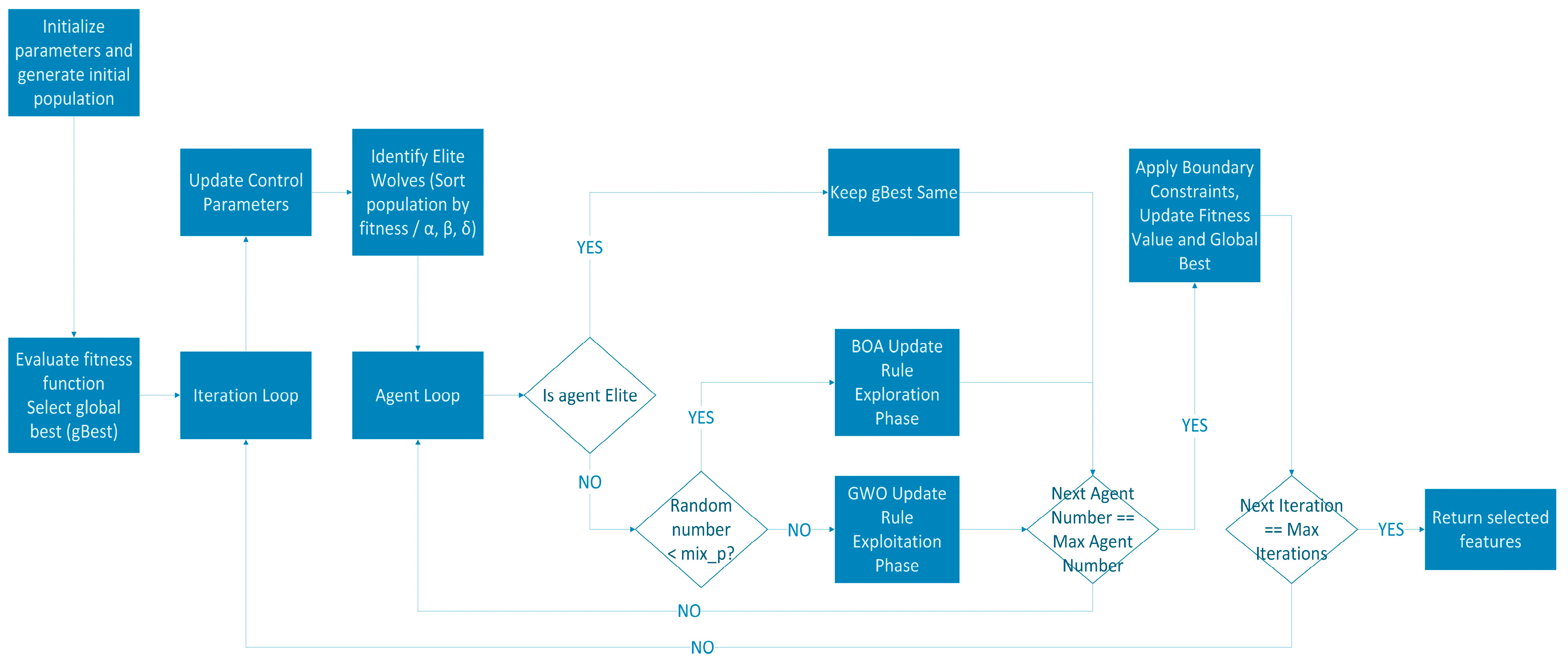
In the hybrid structure developed in this study, either GWO or BOA update mechanism is applied at each iteration with a certain probability. During the BOA phase, agents either move toward the best individual according to the intensity of their fragrance or update their positions relative to other randomly selected butterflies. During GWO phase, agents generate new positions around the alpha (α), beta (β), and delta (δ) individuals, thus converging toward the optimal solution. In this way, the global exploration ability of BOA and the fast convergence advantage of GWO are combined to achieve a more balanced optimization process.

The architecture of the developed model allows for dynamic switching between the two algorithms. As shown in Figure 2, the main objective of this mechanism is to achieve a more effective balance between exploration and evaluation in the search process. The algorithm operates as follows: in each iteration, a random value is generated and compared with the transition probability parameter “mix_p”. If the value is less than “mix_p”, the BOA update rule is applied; otherwise, GWO update rule is executed. Thus, the algorithm alternately benefits from BOA’s strong global exploration capability and GWO’s convergence power at different stages of the optimization.

As a result, the hybrid architecture ensures a more balanced optimization process by integrating both BOA’s exploration ability and GWO’s convergence efficiency. Compared with using BOA or GWO individually, this structure reduces the likelihood of being trapped in local minima and improves the overall robustness of the optimization process.

3.2.2. Evaluation Metrics

The models developed in this study were assessed using the following performance metrics:

• Mean Absolute Error (MAE): the average of absolute differences between predicted and actual values [31].
• Root Mean Squared Error (RMSE): the square root of the average squared differences between predicted and actual values [32].
• Coefficient of Determination (R²): measures how well the regression model explains variance in the dependent variable [33].
• Mean Absolute Percentage Error (MAPE): the average of absolute percentage differences between predicted and actual values, providing a percentage-based measure of prediction accuracy [34].

4. Results

In this study, three different feature-selection models were developed, and regression prediction models were constructed for the target variables using the parameters obtained from these selectors. Experiments were conducted on a workstation equipped with an AMD Ryzen 7 4800H CPU, 16 GB DDR4 RAM, and an NVIDIA RTX 3050 GPU.

All models were implemented in Python 3.10 using PyCharm 2022.2.1 and the scikit-learn, TensorFlow, NumPy, and pandas libraries. The dataset was partitioned into 80% training data and 20% testing data, and fixed random seeds were applied for the data split, metaheuristic executions, and model training to ensure experimental reproducibility. Feature selection was performed once per metaheuristic algorithm, after which ML models were trained using the selected feature subsets. Default scikit-learn parameters were used to ensure a fair baseline comparison, focusing on the impact of feature-selection strategies rather than hyperparameter tuning. Training and inference times were recorded in microseconds using the time.perf_counter() function. Due to high-precision timing, runtime values smaller than 0.0009 s are displayed as 0.000 in the tables for clarity and accuracy.

First, the features selected for the variables Y₁ (heating load) and Y₂ (cooling load) by each feature selector were compared. Subsequently, the performance of the prediction models built with these feature subsets was evaluated using the MAE, RMSE, and R² metrics. Additionally, the fit time and prediction time values were examined to assess the models’ time-performance efficiency. Detailed information on the parameters of the three feature selectors used in the study is presented in

Table 4. Hyperparameters and settings for feature selection algorithms.

Feature Selector	Parameter	Values
GWO	Number of iterations	30
	Population size	20
	Search space lower/upper bounds	0–1
BOA	Number of iterations	30
	Population size	20
	C coefficient (c)	0.01
	Probability (p)	0.8
	Threshold value (thres)	0.25
	α coefficient	0.99
	β coefficient	0.01
	Search space lower/upper bounds	0–1
Hybrid BOA–GWO	Number of iterations	30
	Population size	30
	C coefficient (c)	0.01
	Probability (p)	0.8
	Threshold value (thres)	0.25
	α coefficient	0.99
	β coefficient	0.01
	Search space lower/upper bounds	0–1

.

The GWO algorithm typically has a minimal number of user-defined parameters. Therefore, compared with BOA, only a small amount of parameter tuning was required. It indicates that the algorithm has a simpler, more computationally lightweight structure.

In contrast, the BOA and hybrid BOA–GWO algorithms have more adjustable parameters than the GWO algorithm. In addition to the number of iterations and population size, these algorithms include parameters such as the c coefficient, probability (p), threshold value (thres), and the α and β coefficients. These additional parameters control the exploration–exploitation balance of BOA, which models the butterflies’ scent perception and movement behaviors, and they directly influence the search performance of the algorithm.

Table 5. Feature selection results for output variable Y₁.

Model	Selected Set of Features	Selector Time (s)	Iteration	Population
GWO	‘X1’, ‘X2’, ‘X4’, ‘X5’, ‘X7’	0.5945	30	20
BOA	‘X1’, ‘X2’, ‘X4’, ‘X5’, ‘X7’	0.5344	30	20
Hybrid BOA–GWO	‘X1’, ‘X2’, ‘X4’, ‘X5’, ‘X7’	0.7976	30	30

Note: Y₁ = Heating Load.

and

Table 6. Feature selection results for output variable Y₂.

Model	Selected Set of Features	Selector Time (s)	Iteration	Population
GWO	‘X1’, ‘X5’, ‘X6’, ‘X7’	0.6440	30	20
BOA	‘X1’, ‘X2’, ‘X3’, ‘X4’, ‘X5’, ‘X6’, ‘X7’	0.5550	30	20
Hybrid BOA–GWO	‘X1’, ‘X5’, ‘X7’	0.7976	30	30

Note: Y₂ = Cooling Load.

summarize the features identified by each of the three feature selectors as the most influential for predicting Y₁ (heating load) and Y₂ (cooling load), respectively.

The purpose of applying the three different feature selectors in this study was to identify which attributes were more influential for both Y₁ and Y₂ parameters.

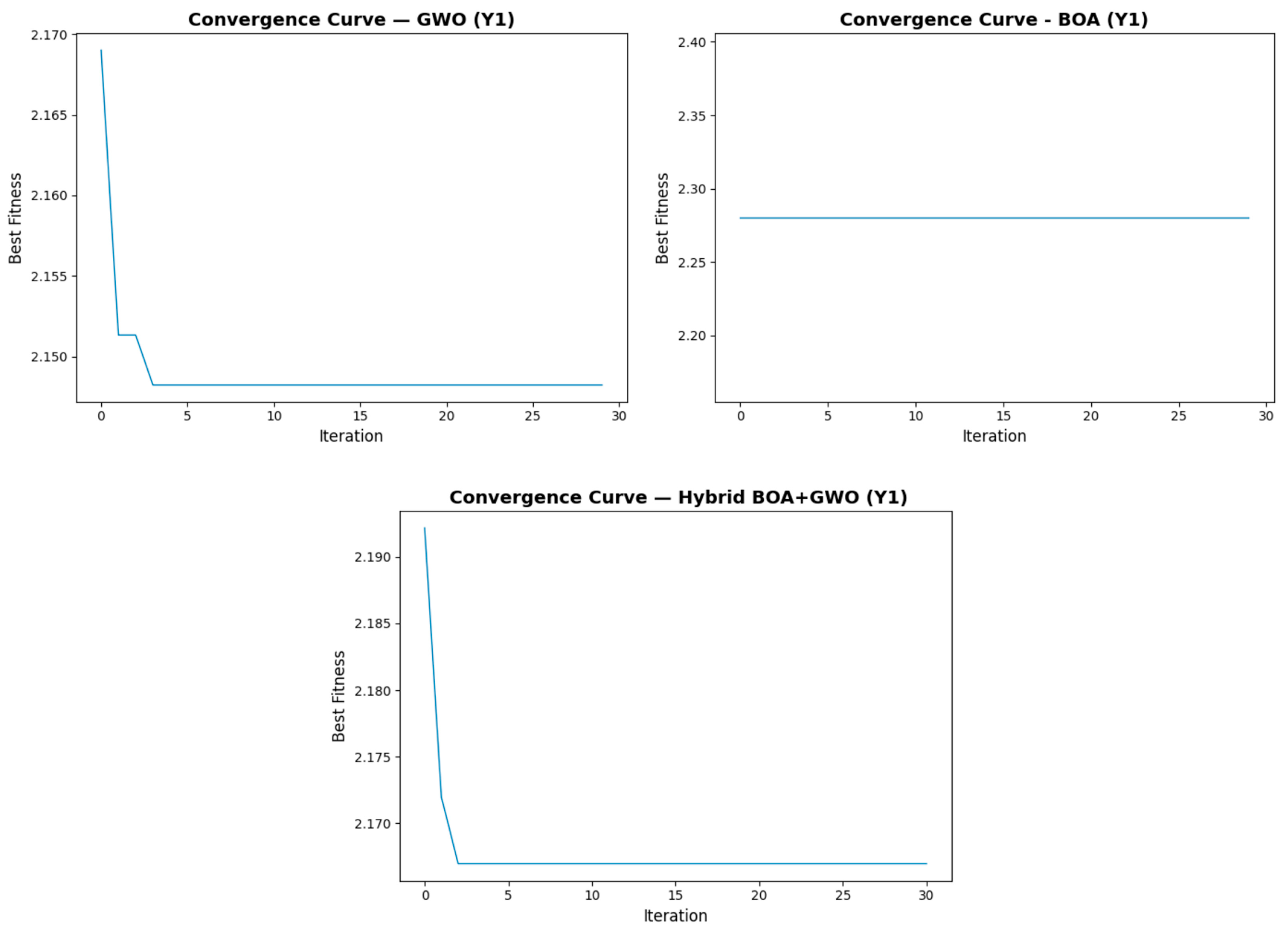
As shown in Table 5, all three feature-selection algorithms identified the same set of features influencing the Y₁ parameter, indicating strong consistency across the applied methods. Each of them selected five out of the eight available features. The unselected features were “Wall Area,” “Orientation,” and “Glazing Area Distribution.” The fact that all three models selected the same set of features demonstrates consistency and emphasizes that the three unselected variables were not as influential as the others. Since the selector execution times were very close and relatively short, all three algorithms can be considered practically applicable in terms of performance. Also, Figure 3 shows the convergence behavior of the feature selectors for feature Y₁. GWO demonstrated compelling exploration of the search space, achieving a better solution in the initial iterations. BOA, in contrast to GWO, produced a constant value across all iterations. The resulting hybrid model, similar to the GWO model, achieved successful results in the initial iterations but found the best solution with a clearer progression.

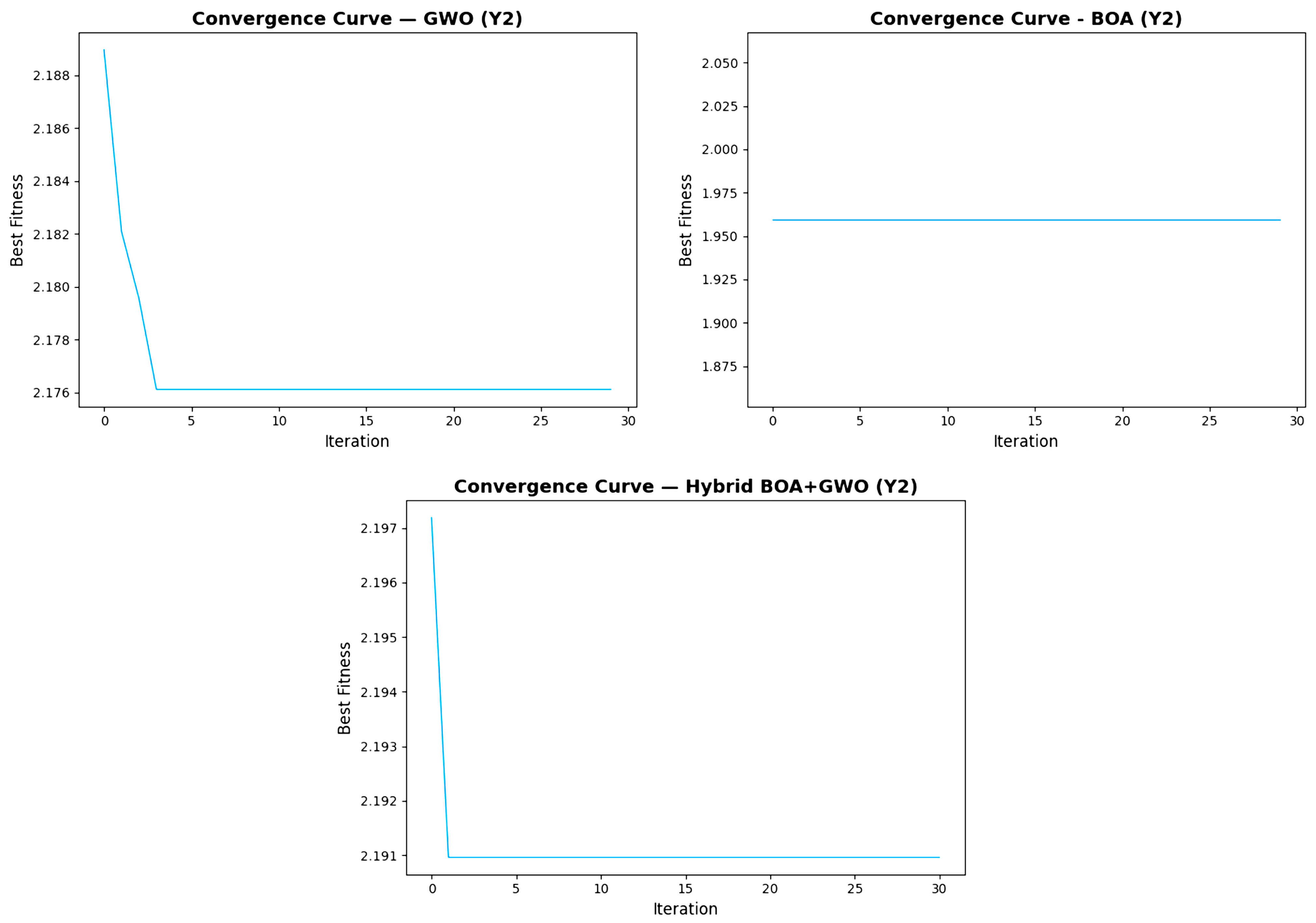
As shown in Table 6, the selection of features influencing the Y₂ parameter differed among the three feature-selection models. The standard variables selected by all models were “Relative Compactness,” “Overall Height,” and “Glazing Area.” It indicates that these three attributes are the most influential features for the Y₂ parameter. The most notable observation is that the BOA model selected all features, implying that, apart from the three standard variables, the contribution of the remaining attributes may vary depending on the model. While the complete agreement among models for Y₁ provides confidence in their consistency, the variation in selected features for Y₂ suggests that the Y₂ parameter exhibits a more complex and multivariate structure. Figure 4 shows the convergence behavior of the feature selectors for feature Y₂. The BOA model exhibits the same behavior for both Y₁ and Y₂. GWO and the hybrid BOA-GWO models progress more smoothly than Y₁. Unlike Y₁, the hybrid model reaches the best solution earlier in Y₂ than the GWO model.

In the study, eight different machine-learning algorithms were also used to construct prediction models. These models were evaluated using three performance metrics: MAE, RMSE, and R². The Y₁ and Y₂ variables were predicted separately, and for each feature subset determined by the three selectors, independent prediction models were developed. To avoid confusion in the results obtained using the evaluation metrics in the study, the four digits after the comma were retained.

After feature selection using the GWO algorithm, all tree-based models achieved nearly identical and excellent R² values for the Y₁ variable. However, as shown in

Table 7. Model performance results for Y₁ using GWO feature selection.

Model	MAE	RMSE	R2	MAPE (%)	Fit Time (s)	Predict Time (s)
LightGBM	0.4360	0.5924	0.9966	2.1808	0.1584	0.0010
CatBoost	0.3728	0.5018	0.9975	1.6625	0.7998	0.0031
Decision Tree (DT)	0.3727	0.5017	0.9975	1.6623	0.0010	0.0010
Random Forest (RF)	0.3739	0.5008	0.9975	1.6671	0.1546	0.0060
Extra Trees (ET)	0.3727	0.5017	0.9975	1.6623	0.0889	0.0052
XGBoost	0.3727	0.5017	0.9975	1.6621	1.5290	0.0020
Linear Regression (LR)	2.1636	3.0361	0.9115	10.2563	0.0010	0.0011
Support Vector Regression (SVR)	5.4286	6.9271	0.5396	28.0182	0.0135	0.0054

Note: For consistency and readability, all numerical results are rounded to four decimal places. Y₁ = Heating Load; GWO = Grey Wolf Optimization Algorithm.

, LightGBM produced the best overall results, while the linear models performed relatively poorly. Additionally, the fit time of XGBoost was observed to be the longest among all models, indicating a higher computational demand during training.

Predictions for both Y₁ and Y₂ were made separately using the features selected by the GWO feature selector. The GWO model utilized five features for Y₁ and four features for Y₂.

As shown in

Table 8. Model performance results for Y₂ using GWO feature selection.

Model	MAE	RMSE	R2	MAPE (%)	Fit Time (s)	Predict Time (s)
LightGBM	1.2170	1.8264	0.9639	4.1746	0.0254	0.0010
CatBoost	1.2392	1.9225	0.9601	4.1685	0.5137	0.0010
Decision Tree (DT)	1.2684	1.9636	0.9583	4.3000	0.0010	0.0010
Random Forest (RF)	1.2723	1.9617	0.9584	4.3027	0.1356	0.0061
Extra Trees (ET)	1.2824	1.9805	0.9576	4.3407	0.0966	0.0071
XGBoost	1.2868	1.9829	0.9575	4.3464	0.0456	0.0010
Linear Regression (LR)	2.1930	3.1577	0.8923	8.5491	0.0010	0.0000
Support Vector Regression (SVR)	3.0809	4.1643	0.8128	11.7960	0.0115	0.0071

Note: Values shown as 0.0000 indicate execution times below 1 × 10⁻⁶ s (timer resolution limit). For consistency and readability, all numerical results are rounded to four decimal places. Y₂ = Cooling Load; GWO = Grey Wolf Optimization Algorithm.

, the LightGBM model achieved the best performance, with an R² value of 0.9639 and a MAPE value of 4.1746. The CatBoost and other tree-based models also produced similarly high and consistent results. In contrast, the linear models (LR and SVR) performed poorly, with R² values below 0.90, indicating a weaker predictive capability compared to the other models. When fit and prediction times are also considered, LightGBM stands out as the model that is both the fastest and the most accurate in predicting energy consumption.

As shown in

Table 9. Model performance results for Y₁ using BOA feature selection.

Model	MAE	RMSE	R2	MAPE (%)	Fit Time (s)	Predict Time (s)
LightGBM	0.4360	0.5924	0.9966	2.1808	0.1106	0.0010
CatBoost	0.3728	0.5018	0.9975	1.6625	0.6556	0.0020
Decision Tree (DT)	0.3727	0.5017	0.9975	1.6623	0.0010	0.0000
Random Forest (RF)	0.3739	0.5008	0.9975	1.6671	0.1145	0.0060
Extra Trees (ET)	0.3727	0.5017	0.9975	1.6623	0.0730	0.0051
XGBoost	0.3727	0.5017	0.9975	1.6621	1.4244	0.0010
Linear Regression (LR)	2.1636	3.0361	0.9115	10.2563	0.0010	0.0000
Support Vector Regression (SVR)	5.4286	6.9271	0.5396	28.0182	0.0111	0.0070

Note: Values shown as 0.0000 indicate execution times below 1 × 10⁻⁶ s (timer resolution limit). For consistency and readability, all numerical results are rounded to four decimal places. Y₁ = Heating Load; BOA = Butterfly Optimization Algorithm.

, the results are highly consistent with those presented in Table 7, as both feature selectors (GWO and BOA) selected the same set of features for the Y₁ parameter. However, when the results for Y₂ are analyzed (

Table 10. Model performance results for Y₂ using BOA feature selection.

Model	MAE	RMSE	R2	MAPE (%)	Fit Time (s)	Predict Time (s)
LightGBM	1.2134	1.8479	0.9631	4.0991	0.0263	0.0005
CatBoost	1.2521	1.9356	0.9595	4.2195	0.5668	0.0011
Decision Tree (DT)	1.2684	1.9636	0.9583	4.3000	0.0010	0.0000
Random Forest (RF)	1.2792	1.9697	0.9581	4.3242	0.1336	0.0053
Extra Trees (ET)	1.2843	1.9801	0.9576	4.3533	0.0911	0.0064
XGBoost	1.2856	1.9894	0.9572	4.3338	0.0492	0.0010
Linear Regression (LR)	2.1991	3.1540	0.8926	8.4924	0.0000	0.0010
Support Vector Regression (SVR)	3.9064	5.2843	0.6986	15.1714	0.0124	0.0060

Note: Values shown as 0.0000 indicate execution times below 1 × 10⁻⁶ s (timer resolution limit). For consistency and readability, all numerical results are rounded to four decimal places. Y₂ = Cooling Load; BOA = Butterfly Optimization Algorithm.

), some differences can be observed. In the BOA-based feature-selection process, seven features were selected. Similar to the GWO results, the LightGBM model achieved the best overall performance with an R² value of 0.9631. When the MAPE values obtained in the Y₁ and Y₂ estimates after applying the BOA feature selector are examined, it is observed that they yield results in parallel with the other error metrics, and LightGBM has the lowest MAPE value. The MAE and RMSE values of the LightGBM model were also lower than those of the other models. In terms of computation, the fit and predict times again showed that LightGBM was the fastest, whereas CatBoost required a longer training duration.

As shown in

Table 11. Model performance results for Y₁ using Hybrid BOA–GWO feature selection.

Model	MAE	RMSE	R2	MAPE (%)	Fit Time (s)	Predict Time (s)
LightGBM	0.4360	0.5924	0.9966	2.1808	0.1442	0.0053
CatBoost	0.3728	0.5018	0.9975	1.6625	0.7503	0.0027
Decision Tree (DT)	0.3727	0.3727	0.9975	1.6623	0.0017	0.0005
Random Forest (RF)	0.3739	0.5008	0.9975	1.6671	0.1116	0.0055
Extra Trees (ET)	0.3727	0.5017	0.9975	1.6623	0.0714	0.0048
XGBoost	0.3727	0.5017	0.9975	1.6621	1.5029	0.0015
Linear Regression (LR)	2.1636	3.0361	0.9115	10.2563	0.0010	0.0000
Support Vector Regression (SVR)	5.4286	6.9271	0.5396	28.0182	0.0130	0.0064

Note: Values shown as 0.0000 indicate execution times below 1 × 10⁻⁶ s (timer resolution limit). For consistency and readability, all numerical results are rounded to four decimal places. Y₁ = Heating Load; BOA–GWO = Butterfly Optimization Algorithm—Grey Wolf Optimization Algorithm.

, the model results are identical to those obtained with the other two feature selectors, demonstrating consistent performance for the Y₁ parameter across all selection methods. However, upon analyzing

Table 12. Model performance results for Y₂ using Hybrid BOA–GWO feature selection.

Model	MAE	RMSE	R2	MAPE (%)	Fit Time (s)	Predict Time (s)
LightGBM	1.1860	1.7495	0.9669	4.0424	0.0288	0.0020
CatBoost	1.1642	1.7464	0.9670	3.9366	0.4860	0.0020
Decision Tree (DT)	1.1653	1.7481	0.9670	3.9410	0.0000	0.0000
Random Forest (RF)	1.1699	1.7489	0.9669	3.9624	0.1010	0.0060
Extra Trees (ET)	1.1653	1.7481	0.9670	3.9410	0.0655	0.0000
XGBoost	1.1653	1.7481	0.9670	3.9408	0.0260	0.0000
Linear Regression (LR)	2.1979	3.1655	0.8918	8.5712	0.0000	0.0000
Support Vector Regression (SVR)	2.9891	4.0867	0.8197	11.3446	0.0060	0.0101

Note: Values shown as 0.0000 indicate execution times below 1 × 10⁻⁶ s (timer resolution limit). For consistency and readability, all numerical results are rounded to four decimal places. Y₂ = Cooling Load; BOA–GWO = Butterfly Optimization Algorithm—Grey Wolf Optimization Algorithm.

, differences become apparent. For Y₂, predictions were made using the three features selected by the hybrid BOA–GWO algorithm. In this case, the best performance was achieved with the CatBoost model, unlike the other feature selectors, where LightGBM had previously shown the best results. While the DT, ET, XGBoost, and RF models produced almost identical levels of accuracy, LightGBM exhibited a slightly higher MAE value. Regarding computation times, Decision Tree, Extra Trees, and XGBoost demonstrated very fast fit durations, confirming their efficiency in training.

Table 13. Model performance results for Y₁ without feature selection.

Model	MAE	RMSE	R2	MAPE (%)	Fit Time (s)	Predict Time (s)
LightGBM	0.3497	0.4786	0.9978	1.6408	0.1320	0.0010
CatBoost	0.2398	0.3352	0.9989	1.0946	0.6961	0.0010
Decision Tree (DT)	0.4248	0.6206	0.9963	1.7474	0.0020	0.0000
Random Forest (RF)	0.3546	0.4907	0.9976	1.4715	0.1608	0.0061
Extra Trees (ET)	0.3533	0.5063	0.9975	1.4725	0.1314	0.0071
XGBoost	0.2635	0.4073	0.9984	1.2687	1.4443	0.0011
Linear Regression (LR)	2.2068	3.0440	0.9111	10.4604	0.0014	0.0000
Support Vector Regression (SVR)	4.2333	5.6543	0.6932	20.4951	0.0120	0.0060

Note: Values shown as 0.0000 indicate execution times below 1 × 10⁻⁶ s (timer resolution limit). For consistency and readability, all numerical results are rounded to four decimal places. Y₁ = Heating Load.

and

Table 14. Model performance results for Y₂ without feature selection.

Model	MAE	RMSE	R2	MAPE (%)	Fit Time (s)	Predict Time (s)
LightGBM	0.7411	1.1236	0.9863	2.5849	0.0264	0.0011
CatBoost	0.4437	0.6746	0.9950	1.6944	0.5606	0.0011
Decision Tree (DT)	1.1551	2.0172	0.9560	4.0622	0.0021	0.0000
Random Forest (RF)	1.0604	1.7129	0.9683	3.5033	0.1648	0.0060
Extra Trees (ET)	1.0445	1.7206	0.9680	3.4825	0.1371	0.0067
XGBoost	0.4486	0.8582	0.9920	1.6180	0.0478	0.0010
Linear Regression (LR)	2.1973	3.1440	0.8933	8.4920	0.0011	0.0000
Support Vector Regression (SVR)	3.9646	5.3516	0.6908	15.3963	0.0136	0.0060

Note: Values shown as 0.0000 indicate execution times below 1 × 10⁻⁶ s (timer resolution limit). For consistency and readability, all numerical results are rounded to four decimal places. Y₂ = Cooling Load.

present the results obtained without applying feature selection, i.e., when all features were used in model training. When Table 13 is examined for the Y₁ parameter, it can be observed that the CatBoost model achieved the lowest error values, with MAE = 0.2398, RMSE = 0.3352, R² = 0.9989, and MAPE = 1.0946. Both XGBoost and LightGBM also demonstrated performances very close to CatBoost, confirming the strong predictive power of gradient boosting methods. The linear models (LR and SVR), on the other hand, once again underperformed compared to tree-based algorithms, indicating their limited ability to model nonlinear relationships within the dataset.

As shown in Table 14, the best performance for the Y₂ parameter was again achieved with the CatBoost model, with MAE = 0.4437, RMSE = 0.6746, R² = 0.9950, and MAPE = 1.6944. Although XGBoost achieved a similarly high R² value, DT, RF, and ET models showed higher error rates, indicating slightly weaker predictive performance. Once again, the LR and SVR models demonstrated poor results, confirming that linear algorithms are not suitable for accurately capturing the nonlinear relationships in the building energy consumption data.

The gradient boosting–based tree models achieved the lowest errors and highest R² values for both Y₁ and Y₂ predictions in all cases. In particular, the CatBoost model consistently delivered the best or nearly best performance across all tables. In contrast, the linear models showed weak performance without feature selection, although their predictive accuracy improved slightly when feature selection was applied.

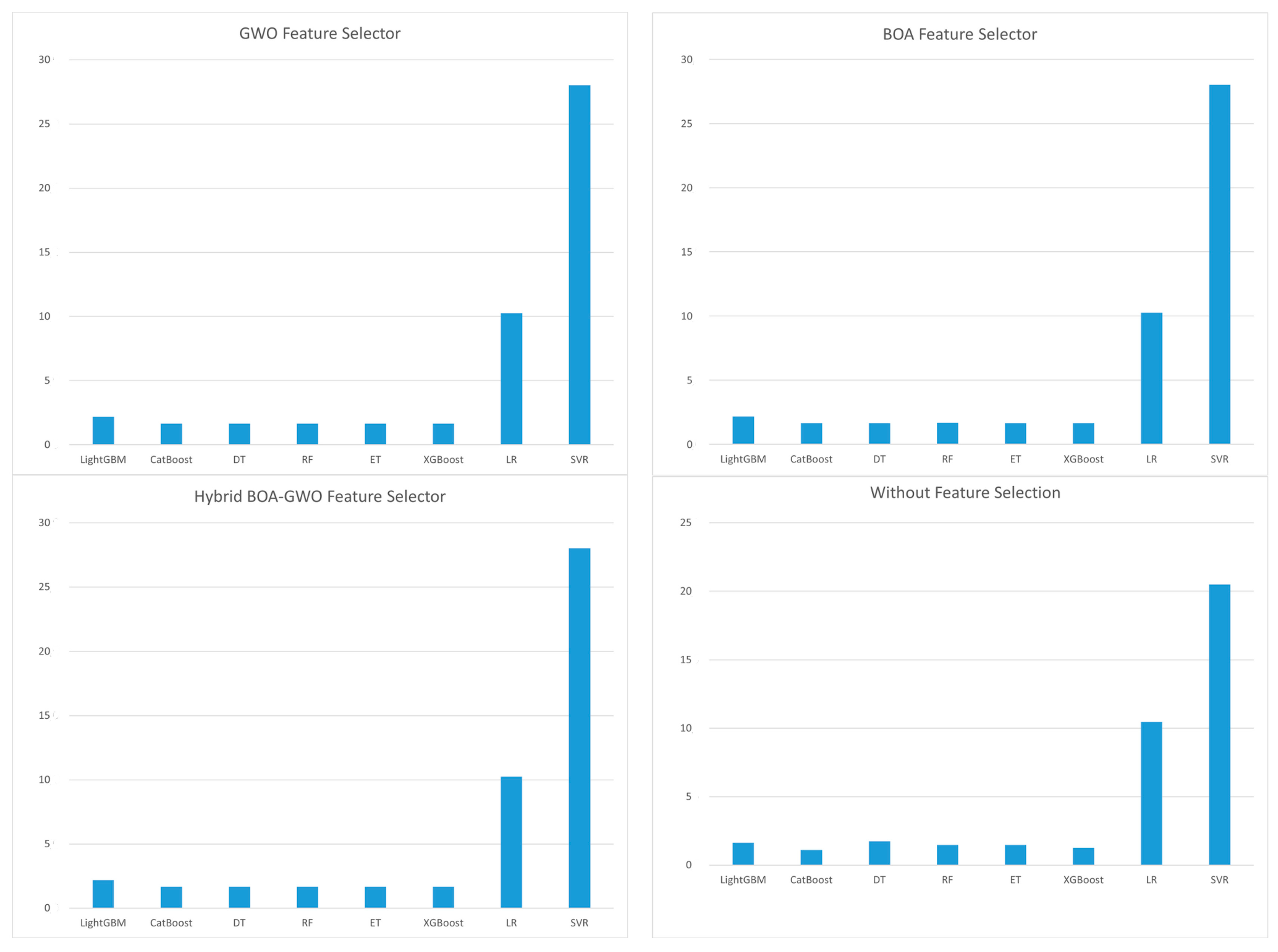
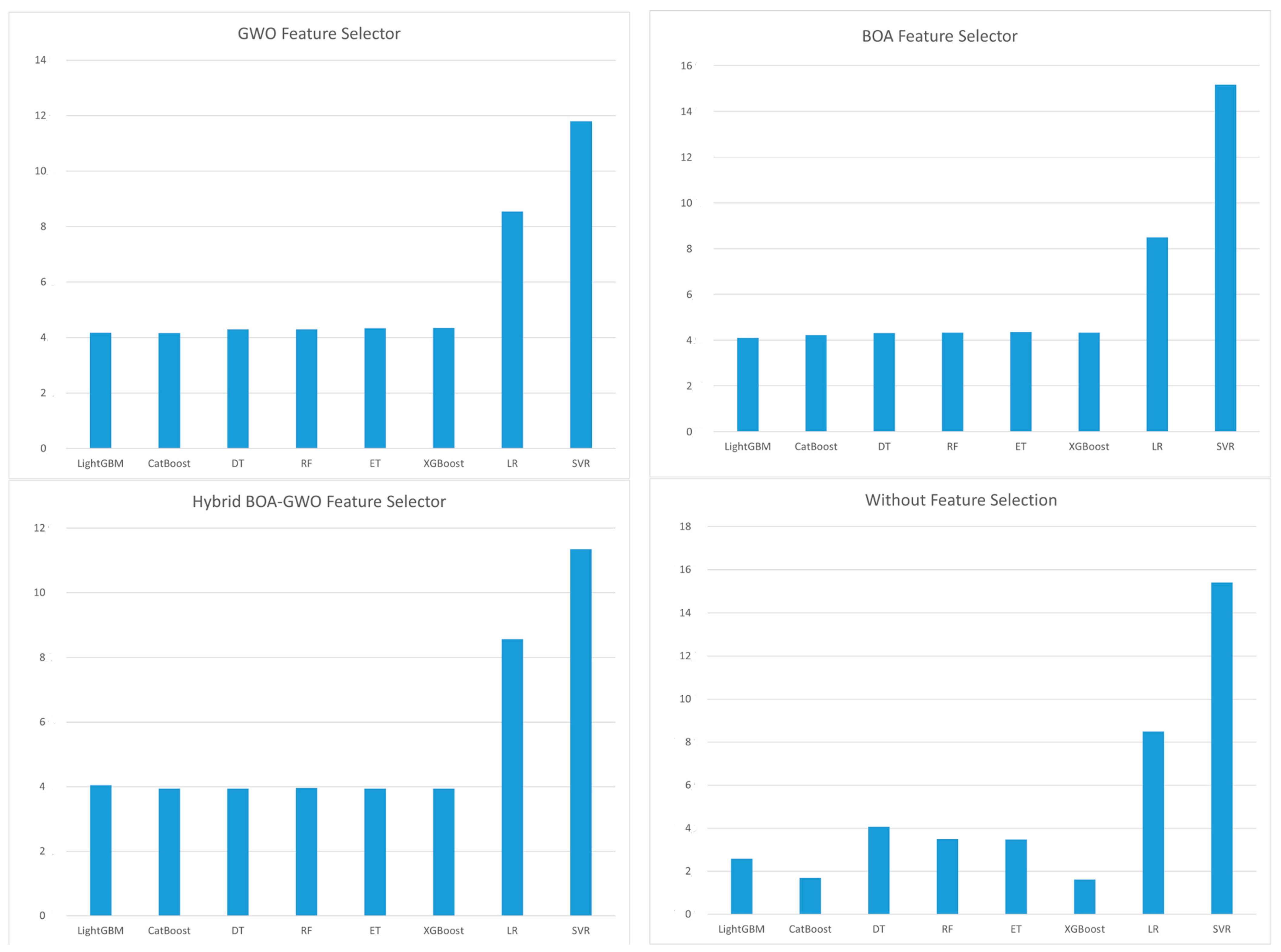
MAPE’s normalization of errors as a percentage enables a more objective interpretation by presenting the prediction accuracy of models with different structures from a unified perspective. Therefore, for unbiased comparison of models, Figure 5 and Figure 6 display histograms showing the MAPE values obtained by the models in each scenario. An examination of the figures reveals that gradient descent-based models achieve the lowest MAPE values for both Y₁ and Y₂. In contrast, linear models exhibit poorer performance. Moreover, the statistics illustrate that tree-based ensemble methods yield more reliable and stable predictions, while feature selection further enhances model performance without compromising computational efficiency.

Applying feature selection to Y₁ and Y₂ resulted in different numbers of selected features: five were consistently chosen for Y₁, while the subset for Y₂ varied depending on the feature-selection algorithm. In several models, especially for Y₂, slight improvements in prediction accuracy were observed, indicating that the selected features were indeed informative and relevant to the target variables.

While the BOA tended to select a larger number of features and GWO focused on a smaller subset, the hybrid BOA–GWO algorithm balanced exploration and exploitation, producing a more compact yet highly predictive feature subset. This balance reduced model complexity without sacrificing accuracy, particularly for the cooling load (Y₂) variable; with the hybrid approach, the R² value increased from 0.9631 (BOA) and 0.9639 (GWO) to 0.9670.

In terms of the performance–time trade-off, LightGBM achieved the fastest training times with strong performance, while CatBoost provided the highest accuracy, albeit with slightly longer training durations. The classical linear models produced results quickly but had significantly lower accuracy.

5. Discussion

The findings of this study are consistent with those reported by Bassi et al. [10], who demonstrated that gradient boosting models such as XGBoost, LightGBM, and CatBoost outperform classical regression techniques for building energy prediction. Similarly, Afzal et al. [17] showed that hybrid models integrating neural networks with optimization algorithms yield higher accuracy compared to standalone models. Aligned with these studies, the results of the present research confirm the superior performance of gradient boosting methods, with CatBoost achieving the highest accuracy (mostly R² > 0.99).

However, unlike previous studies that primarily focused on accuracy metrics [16,19], this research extends the analysis by incorporating training time, prediction time, and feature efficiency into a multi-criteria evaluation. This comprehensive assessment reveals that while CatBoost provides the highest predictive accuracy, LightGBM achieves comparable accuracy with faster training, and the proposed hybrid BOA–GWO feature selector enhances efficiency without compromising performance.

In addition to improving predictive performance, feature selection also enhances model interpretability by highlighting the parameters that influence building energy consumption. In building energy management, understanding which physical characteristics, such as overall height, relative compactness, or glazing area, influence heating and cooling loads allows facilities management to make more informed decisions about design and control strategies.

These outcomes confirm that integrating metaheuristic optimization with machine learning provides a robust, accurate, and efficient method for predicting energy consumption, supporting both academic and practical advancements in sustainable building management.

5.1. Comparison with Existing Smart Building Energy Management Approaches

Previous research in smart energy management has predominantly relied on deep learning or reinforcement learning–based models for load forecasting and energy optimization in IoT-enabled buildings. While these approaches can achieve high predictive accuracy, they typically require substantial computational resources, frequent retraining, and access to large-scale real-world datasets. The proposed BOA–GWO–supported gradient boosting framework prioritizes computational efficiency and compact feature selection, making it ideal for embedded smart building environments. It complements existing deep-learning-based solutions by providing a lightweight and efficient alternative for real-time energy prediction under resource constraints.

This emphasis on computational efficiency is consistent with findings in recent smart building studies, which highlight that deep-learning-based approaches, while accurate, often require substantial processing power and frequent retraining, making lightweight ML-based solutions more suitable for embedded and IoT environments [35,36].

5.2. Dataset Limitations and Generalizability

This study utilized the UCI Energy Efficiency dataset [12], which consists of 768 simulated residential building samples defined by eight input features and two continuous target variables (heating and cooling loads). Although this dataset is widely used as a benchmark in the literature, it contains inherent limitations that may introduce bias in model generalization. Specifically, it represents only simulated residential buildings with fixed geometric and thermal parameter ranges and balanced heating/cooling load distributions, which do not fully reflect the diversity of real-world building stock, including commercial and mixed-use facilities, varying climate zones, and heterogeneous occupancy and operational conditions. Such restricted variability may lead to optimistic performance within this benchmark setting and insufficient representation of extreme or irregular behaviors observed in actual building energy systems. Therefore, the promising predictive accuracy and computational efficiency achieved by the proposed hybrid BOA–GWO framework should be interpreted as preliminary rather than definitive evidence of real-world generalizability.

Furthermore, the dataset consists of static building attributes rather than time-series energy consumption data. As a result, the proposed model predicts energy loads for buildings with similar architectural and thermal characteristics rather than forecasting future energy consumption trajectories. It enables controlled performance evaluation but does not account for temporal dynamics, operational variability, or adaptive behavior in real-time systems.

Future work will therefore focus on applying the hybrid BOA–GWO approach to real-time building datasets and time-series energy consumption models. It will enable the assessment of its performance across diverse climates, building typologies, operational scenarios, and dataset scales, as well as the evaluation of its short- and long-term forecasting capability, adaptive learning performance, and suitability for real-time smart building and IoT-enabled applications.

For clarity, dataset-related limitations are summarized in

Table 15. Dataset-related limitations considered in this study.

Limitation	Impact on Results	Future Direction
Single benchmark dataset (UCI)	Limited generalizability to wider building stock	Validate on multiple real-world datasets
Residential-simulated buildings only	Cannot represent commercial/mixed-use operations	Include commercial & mixed-use samples
Static architectural & thermal variables (no time-series data)	Predicts loads for similar buildings but not future consumption	Extend to real-time & time-series IoT/sensor data
Balanced heating-cooling distribution	Potential optimistic performance vs. real load imbalance	Use datasets with natural imbalance
No occupancy, climate, or HVAC operation dynamics	Does not reflect operational variability	Integrate dynamic environmental & operational variables

.

6. Conclusions

This study successfully proposes a hybrid approach that integrates nature-inspired feature selection algorithms (GWO, BOA, and Hybrid BOA–GWO) with robust gradient boosting machine-learning methods (LightGBM, CatBoost, and XGBoost) to improve the predictive performance of building heating (Y₁) and cooling (Y₂) loads using the UCI Energy Efficiency dataset. Unlike studies that focus solely on optimizing ML models, the primary contribution here is improving predictive performance through a hybrid feature-selection strategy. Secondary considerations included training time and feature compactness to assess real-world applicability.

The key findings demonstrate that integrating nature-inspired feature-selection algorithms with machine-learning methods improves both predictive accuracy and computational efficiency. Comparisons of model fit and prediction times further revealed that hybrid approaches achieved higher accuracy in shorter time than classical methods. For the heating load (Y₁), all models consistently selected the same features, indicating their strong influence on prediction. In contrast, the variability in the features chosen for the cooling load (Y₂) suggests a more complex, multivariate structure. Overall, combining nature-inspired feature selection with gradient-boosting models provides a computationally efficient, highly accurate, and straightforward approach for predicting building energy loads. It demonstrates that accuracy, computational speed, and model simplicity can be jointly optimized for real-time and resource-constrained smart-building applications.

The proposed hybrid BOA–GWO feature selection algorithm leverages the global exploration capability of BOA and the local exploitation ability of GWO, producing a balanced, compact, and highly predictive feature set. When combined with XGBoost, it achieved the best performance for Y₂ prediction (R² ≈ 0.967) using only three features, demonstrating high predictive accuracy with reduced computational cost and model complexity. In addition to the accuracy improvements achieved with gradient boosting methods, the hybrid approach outperformed the individual BOA and GWO implementations. It provides efficiency and stability, making it especially suitable for real-time, resource-constrained applications such as IoT-based energy management and smart building systems.

To the best of our knowledge, while hybrid BOA–GWO schemes have been explored in other computational intelligence domains, this study represents one of the first applications of a BOA–GWO–based feature-selection framework specifically for building energy consumption prediction. Rather than introducing a new metaheuristic, it adapts the BOA–GWO hybrid logic to the building energy domain and evaluates performance from a multi-criteria perspective, including accuracy, training time, and feature compactness. This domain-oriented adaptation and comprehensive evaluation offer practical value for real-time and resource-constrained smart building environments.

Despite the promising results, this study has certain limitations. The UCI Energy Efficiency dataset, although widely used in the literature, does not fully reflect the diversity and scale of real-world building energy data. It includes only simulated residential buildings with fixed geometric and thermal parameter ranges and balanced heating/cooling loads, which may not reflect mixed-use or commercial buildings, different climatic zones, or dynamic operational conditions. Additionally, the dataset contains static building features rather than time-dependent consumption patterns; therefore, the model predicts energy loads for buildings with similar characteristics, rather than forecasting temporal energy demand. Thus, the results and conclusions drawn from this single dataset should be interpreted with caution and cannot be directly generalized to broader real-world scenarios or large-scale IoT-based applications. Furthermore, because the research is based on a single benchmark dataset, it may not accurately reflect the diversity of actual building energy usage across various climates and building categories.

Additionally, since the primary focus of this research was to evaluate the effectiveness of hybrid feature-selection strategies rather than hyperparameter optimization, all ML models were trained with default parameter configurations. Future work should validate the hybrid BOA–GWO framework on larger and more diverse datasets, including commercial and industrial buildings across various climatic conditions and dynamic operational profiles. Integrating additional nature-inspired algorithms or deep-learning-based hybrid approaches, as well as conducting systematic hyperparameter tuning, could further improve performance and generalizability. Moreover, although the proposed nature-based feature selectors have demonstrated strong predictive performance, future studies may compare them with classical baselines such as Least Absolute Shrinkage and Selection Operator (LASSO) regression, Recursive Feature Elimination (RFE), and tree-based feature-importance metrics. Reporting the mean and standard deviation of evaluation metrics across multiple runs with different random seeds on more comprehensive benchmark datasets would also strengthen the robustness and reproducibility of the results. Finally, applying the model to time-series and real-time energy data streams will enable the assessment of its short- and long-term forecasting capabilities, adaptive learning potential, and suitability for IoT-enabled smart grid environments.

References

1. Jing, Q.; Guo, Y.; Liu, Y.; Wang, Y.; Du, C.; Liu, X. Optimization Study of Energy Saving Control Strategy of Carbon Dioxide Heat Pump Water Heater System under the Perspective of Energy Storage. Appl. Therm. Eng. 2026, 283, 129030. [Google Scholar] [CrossRef]
2. United Nations Environment Programme; Global Alliance for Buildings and Construction. Not Just Another Brick in the Wall: The Solutions Exist—Scaling Them Will Build on Progress and Cut Emissions Fast. Global Status Report for Buildings and Construction 2024/2025; UNEP/GlobalABC: Paris, France, 2025. [Google Scholar]
3. International Energy Agency. Net Zero by 2050—A Roadmap for the Global Energy Sector; International Energy Agency: Paris, France, 2021. [Google Scholar]
4. Bibri, S.E.; Huang, J.; Omar, O.; Kenawy, I. Synergistic Integration of Digital Twins and Zero Energy Buildings for Climate Change Mitigation in Sustainable Smart Cities: A Systematic Review and Novel Framework. Energy Build. 2025, 333, 115484. [Google Scholar] [CrossRef]
5. Deb, C.; Zhang, F.; Yang, J.; Lee, S.E.; Shah, K.W. A Review on Time Series Forecasting Techniques for Building Energy Consumption. Renew. Sustain. Energy Rev. 2017, 74, 902–924. [Google Scholar] [CrossRef]
6. Ul Haq, M.S.; Ji, W.; Pei, X.; Liu, S.; Geng, Y.; Lin, B.; Ali, H. Explainable Deep Learning Combined Attention-Based LSTM for Building Energy Prediction: A Framework from the Perspective of Supply Side. Energy Build. 2026, 350, 116638. [Google Scholar] [CrossRef]
7. Eslamirad, N.; Golamnia, M.; Sajadi, P.; Pilla, F. Leveraging Machine Learning for Data-Driven Building Energy Rate Prediction. Results Eng. 2025, 26, 104931. [Google Scholar] [CrossRef]
8. Kausik, A.K.; Rashid, A.B.; Baki, R.F.; Jannat Maktum, M.M. Machine Learning Algorithms for Manufacturing Quality Assurance: A Systematic Review of Performance Metrics and Applications. Array 2025, 26, 100393. [Google Scholar] [CrossRef]
9. Mirjalili, S.; Mirjalili, S.M.; Lewis, A. Grey Wolf Optimizer. Adv. Eng. Softw. 2014, 69, 46–61. [Google Scholar] [CrossRef]
10. Bassi, A.; Shenoy, A.; Sharma, A.; Sigurdson, H.; Glossop, C.; Chan, J.H. Building Energy Consumption Forecasting: A Comparison of Gradient Boosting Models. In Proceedings of the IAIT2021: The 12th International Conference on Advances in Information Technology, Bangkok, Thailand, June 29–1 July 2021. ACM International Conference Proceeding Series. [Google Scholar] [CrossRef]
11. Zhao, H.X.; Magoulès, F. A Review on the Prediction of Building Energy Consumption. Renew. Sustain. Energy Rev. 2012, 16, 3586–3592. [Google Scholar] [CrossRef]
12. Tsanas, A.; Xifara, A. Accurate Quantitative Estimation of Energy Performance of Residential Buildings Using Statistical Machine Learning Tools. Energy Build. 2012, 49, 560–567. [Google Scholar] [CrossRef]
13. Ghasemkhani, B.; Yilmaz, R.; Birant, D.; Kut, R.A. Machine Learning Models for the Prediction of Energy Consumption Based on Cooling and Heating Loads in Internet-of-Things-Based Smart Buildings. Symmetry 2022, 14, 1553. [Google Scholar] [CrossRef]
14. Al-Essa, L.A.; Ebrahim, E.A.; Mergiaw, Y.A. Bayesian Regression Modeling and Inference of Energy Efficiency Data: The Effect of Collinearity and Sensitivity Analysis. Front. Energy Res. 2024, 12, 1416126. [Google Scholar] [CrossRef]
15. Aly, M.; Alotaibi, A.S. Hybrid Butterfly-Grey Wolf Optimization (HB-GWO): A Novel Metaheuristic Approach for Feature Selection in High-Dimensional Data. Stat. Optim. Inf. Comput. 2025, 13, 2575–2600. [Google Scholar] [CrossRef]
16. Somu, N.; Gauthama Raman, M.R.; Ramamritham, K. A Hybrid Model for Building Energy Consumption Forecasting Using Long Short Term Memory Networks. Appl. Energy 2020, 261, 114131. [Google Scholar] [CrossRef]
17. Afzal, S.; Shokri, A.; Ziapour, B.M.; Shakibi, H.; Sobhani, B. Building Energy Consumption Prediction and Optimization Using Different Neural Network-Assisted Models; Comparison of Different Networks and Optimization Algorithms. Eng. Appl. Artif. Intell. 2024, 127, 107356. [Google Scholar] [CrossRef]
18. Zheng, S.; Liu, S.; Zhang, Z.; Gu, D.; Xia, C.; Pang, H.; Ampaw, E.M. TRIZ Method for Urban Building Energy Optimization: GWO-SARIMA-LSTM Forecasting Model. J. Intell. Technol. Innov. (JITI) 2024, 2, 78–103. [Google Scholar] [CrossRef]
19. Ghalambaz, M.; Jalilzadeh Yengejeh, R.; Davami, A.H. Building Energy Optimization Using Grey Wolf Optimizer (GWO). Case Stud. Therm. Eng. 2021, 27, 101250. [Google Scholar] [CrossRef]
20. Ilbeigi, M.; Ghomeishi, M.; Dehghanbanadaki, A. Prediction and Optimization of Energy Consumption in an Office Building Using Artificial Neural Network and a Genetic Algorithm. Sustain. Cities Soc. 2020, 61, 102325. [Google Scholar] [CrossRef]
21. Amasyali, K.; El-Gohary, N.M. A Review of Data-Driven Building Energy Consumption Prediction Studies. Renew. Sustain. Energy Rev. 2018, 81, 1192–1205. [Google Scholar] [CrossRef]
22. Sun, X.; Liu, M.; Sima, Z. A Novel Cryptocurrency Price Trend Forecasting Model Based on LightGBM. Financ. Res. Lett. 2020, 32, 101084. [Google Scholar] [CrossRef]
23. Zhai, W.; Li, C.; Fei, S.; Liu, Y.; Ding, F.; Cheng, Q.; Chen, Z. CatBoost Algorithm for Estimating Maize Above-Ground Biomass Using Unmanned Aerial Vehicle-Based Multi-Source Sensor Data and SPAD Values. Comput. Electron. Agric. 2023, 214, 108306. [Google Scholar] [CrossRef]
24. Pekel, E. Estimation of Soil Moisture Using Decision Tree Regression. Theor. Appl. Climatol. 2020, 139, 1111–1119. [Google Scholar] [CrossRef]
25. Wang, F.; Wang, Y.; Zhang, K.; Hu, M.; Weng, Q.; Zhang, H. Spatial Heterogeneity Modeling of Water Quality Based on Random Forest Regression and Model Interpretation. Environ. Res. 2021, 202, 111660. [Google Scholar] [CrossRef] [PubMed]
26. Jafari, S.; Byun, Y.C. Efficient State of Charge Estimation in Electric Vehicles Batteries Based on the Extra Tree Regressor: A Data-Driven Approach. Heliyon 2024, 10, e25949. [Google Scholar] [CrossRef] [PubMed]
27. Zhang, X.; Yan, C.; Gao, C.; Malin, B.A.; Chen, Y. Predicting Missing Values in Medical Data Via XGBoost Regression. J. Healthc. Inform. Res. 2020, 4, 383–394. [Google Scholar] [CrossRef]
28. Fedotova, O.; Teixeira, L.; Alvelos, H. Software Effort Estimation with Multiple Linear Regression: Review and Practical Application. J. Inf. Sci. Eng. 2013, 29, 925–945. [Google Scholar]
29. Fan, G.F.; Yu, M.; Dong, S.Q.; Yeh, Y.H.; Hong, W.C. Forecasting Short-Term Electricity Load Using Hybrid Support Vector Regression with Grey Catastrophe and Random Forest Modeling. Util. Policy 2021, 73, 101294. [Google Scholar] [CrossRef]
30. Makhadmeh, S.N.; Al-Betar, M.A.; Abasi, A.K.; Awadallah, M.A.; Doush, I.A.; Alyasseri, Z.A.A.; Alomari, O.A. Recent Advances in Butterfly Optimization Algorithm, Its Versions and Applications. Arch. Comput. Methods Eng. 2023, 30, 1399–1420. [Google Scholar] [CrossRef]
31. Willmott, C.J.; Matsuura, K. Advantages of the Mean Absolute Error (MAE) over the Root Mean Square Error (RMSE) in Assessing Average Model Performance. Clim. Res. 2005, 30, 79–82. [Google Scholar] [CrossRef]
32. Hodson, T.O. Root-Mean-Square Error (RMSE) or Mean Absolute Error (MAE): When to Use Them or Not. Geosci. Model. Dev. 2022, 15, 5481–5487. [Google Scholar] [CrossRef]
33. Gao, J. R-Squared (R2)—How Much Variation Is Explained? Res. Methods Med. Health Sci. 2024, 5, 104–109. [Google Scholar] [CrossRef]
34. Montaño Moreno, J.J.; Palmer Pol, A.; Sesé Abad, A.; Cajal Blasco, B. El Índice R-MAPE Como Medida Resistente Del Ajuste En La Previsión. Psicothema 2013, 25, 500–506. [Google Scholar] [CrossRef] [PubMed]
35. Runge, J.; Zmeureanu, R. A Review of Deep Learning Techniques for Forecasting Energy Use in Buildings. Energies 2021, 14, 608. [Google Scholar] [CrossRef]
36. Li, D.; Qi, Z.; Zhou, Y.; Elchalakani, M. Machine Learning Applications in Building Energy Systems: Review and Prospects. Buildings 2025, 15, 648. [Google Scholar] [CrossRef]
Figure 1. Distribution of Heating (Y1) and Cooling Loads (Y2).
Sustainability 17 10718 g001
Figure 2. Flowchart of hybrid BOA-GWO.
Sustainability 17 10718 g002
Figure 3. Convergence performance comparison of feature selectors for Heating Load (Y1).
Sustainability 17 10718 g003
Figure 4. Convergence performance comparison of feature selectors for Heating Load (Y2).
Sustainability 17 10718 g004
Figure 5. MAPE comparison of models for Heating Load (Y1).
Sustainability 17 10718 g005
Figure 6. MAPE comparison of models for Heating Load (Y2).
Sustainability 17 10718 g006