Predicting Urban Traffic Congestion Through Deterministic and Stochastic Modeling Using LSTM Neural Networks

Abstract

Urban traffic congestion leads to significant economic losses, increased air pollution, and reduced quality of life, making its prediction and mitigation a critical task for sustainable urban development. Traditional prediction methods are often not integrated with real-time monitoring data, which limits their practical applicability. To bridge this gap, this paper proposes a novel approach that combines deterministic and stochastic simulation modeling to predict traffic congestion of varying complexity. The approach is based on a simulation model developed in the Matlab Simulink environment. The model uses real data from the AIMS eco software package, which provides real-time traffic monitoring. The simulation experiments demonstrated the dynamics of congestion formation and dissipation under various scenarios. Based on these experiments, a neural network (based on LSTM) was developed and trained on an extended dataset to predict the growth of queue length. The LSTM model achieved high accuracy in predicting queue dynamics, with a mean absolute error (MAE) of 1.5 vehicles for the number of vehicles unable to pass through the intersection per cycle and 0.3 vehicles for the total queue size. The developed model represents an effective tool for analyzing and predicting traffic congestion, thereby providing a scientific foundation for integrating a predictive module into intelligent transportation systems (ITS) such as AIMS eco.

1. Introduction

Urban traffic congestion remains one of the most pressing challenges in modern urban planning, with multifaceted negative impacts on the environment, the economy, and quality of life. A critical consequence of congestion is the significant deterioration of the urban environment. Idling and unsteady engine operation can increase pollutant emissions by 30% or more, posing a direct threat to the health of city residents [1,2,3,4]. Despite the existence of various mathematical models describing traffic congestion dynamics, their practical application is often limited by the lack of integration with real-time traffic monitoring systems [5,6,7,8]. Traditional approaches to congestion prediction demonstrate insufficient effectiveness when processing large volumes of heterogeneous data from modern intelligent transportation systems. This creates a significant gap between theoretical developments and their practical implementation in urban mobility management systems.

Congestion conditions vary greatly in their causes and contributing factors, scale, and duration. While there is no official classification of congestion, many authors offer their own classifications. Based on generalizations, a simple classification can be proposed: non-recurrent (random) and recurrent (pulsating) congestion [9,10,11,12].

Non-recurrent congestion occurs at unexpected locations along the road network and is typically caused by major incidents, such as accidents, the clearance of which can require up to 3–4 h. During such events, roadway capacity can decrease by 50 or even come to a complete standstill [13,14,15]. Similar situations arise from failures of underground utilities (e.g., water mains, gas pipelines, or electrical systems), requiring immediate emergency response and resulting in full or partial road closures.

Recurrent traffic congestion typically occurs in the same locations, most often at traffic signal intersections that are unable to handle the required traffic volume, or at sites of prolonged roadside repairs with closed road sections. Such congestion often not constitute a complete standstill but rather a pulsating flow that moves forward during green phases.

Traffic congestion, like any traffic delay, lead to economic losses, including time losses for passengers and vehicle owners, reduced efficiency of freight transportation, and increased fuel consumption [16]. It also contributes to a higher incidence of accidents (particularly rear-end collisions) and increases driver stress [17]. However, the most significant negative consequence of traffic congestion, especially in urban areas, is their severely negative impact on the environment. Increased fuel consumption, combined with a high proportion of stop-and-go driving and engine idling, can raise pollutant emissions by 30% or more, posing a substantial threat to human health [18,19,20,21].

Congestion is characterized by its duration and the number of vehicles involved. The latter can be estimated based on the queue length and the traffic density when vehicles are stationary.

In a slow-moving vehicle queue within a zone of complete traffic congestion, the negative environmental impact approaches that of a total standstill, while the economic indicators of the transportation process deteriorate significantly compared to standard norms. Therefore, many researchers and experts believe such a flow to be in a traffic congestion. They define the lower speed threshold for this state as 10–15 km/h (corresponding to a travel time of 4–6 min/km) [22,23].

Addressing the problem of congestion mitigation first requires identifying locations where congestion is expected and symptoms of insufficient capacity of road network nodes (congestion) are already present. This task can be most reliably solved through comprehensive monitoring. This task can be most effectively solved through comprehensive monitoring. Video surveillance using stationary street cameras is a highly effective method for collecting such information, as it is particularly adept at detecting congestion origins [24,25]. Owing to the ongoing development of Intelligent Transportation Systems (ITS), diverse traffic data sources provide substantial information volumes [26]. These big data are used to develop models for predicting various traffic conditions. Accurate prediction enables city transport services to take timely measures to mitigate traffic congestion [27,28].

The aim of this study is to develop a methodology for predicting traffic congestion of varying complexity based on the integration of simulation modeling and deep learning. To achieve this goal, the following tasks were set: (1) developing a simulation model of congestion formation in the MATLAB/Simulink (Math Works-Simulink R2014b) environment; (2) creating an LSTM model for predicting vehicle queue growth; and (3) verifying the developed models using real-world traffic monitoring data.

This paper presents the development of a simulation model for predicting traffic congestion of varying complexity at urban intersections. The AIMS eco “Real-Time Vehicle Emissions Monitoring System” software package (https://aims.susu.ru/demo/dashboard/chelyabinsk/city accessed on 1 October 2025) [29] serves as the primary data source for the model.

2. Related Work

Ye et al. [30] studied the factors of urban traffic congestion heterogeneity: population density and the location of the business district affect road congestion, while an increase in the number of bus stops reduces traffic congestion. Zhao et al. [31] addressed the problem of short-term congestion prediction by applying a Self-Organizing Feature Map (SOFM) model to classify congestion levels based on a system of indices. Similarly, building on traffic efficiency indices and the self-organizing map method, a study [32] proposed clustering traffic congestion patterns for different day types, including Mondays, Fridays, weekdays, weekends, and holidays. For short-term forecasting (30 min) of traffic flow (TF) at a signalized intersection, Qu et al. [33] compared a KNN regression model, a clustering-based algorithm, and two neural network models. Their findings indicate that such forecasting can enable users to plan trips and facilitate appropriate traffic management measures.

Elleuch et al. [34] developed a traffic congestion classification system (categorizing states into light, moderate, and heavy traffic) based on spectrograms derived from traffic videos and a neural network. Gatto and Forster [35] utilized sound sensors combined with machine learning for traffic monitoring.

In recent years, the continuous advancement of deep learning has led to the increasing adoption of neural network-based models for traffic forecasting [36,37]. Ma et al. [38] proposed a Long Short-Term Memory (LSTM) neural network for traffic flow analysis. The proposed model demonstrated superior accuracy and stability compared to other common algorithms.

Similarly, to predict traffic congestion occurrence, a study [39] implemented an LSTM model using data from vehicle detectors. Liu et al. [40] detected traffic congestion by analyzing transformed online road images, employing a deep graph convolutional neural network for prediction. A deep graph process model for predicting traffic congestions complexity in urban transport environments was presented in [41]. The traffic congestion early warning system introduced in [42] integrated point prediction, TF parameter characteristic estimation, interval prediction, and a comprehensive assessment of the overall road congestion level.

Recently, researchers have enhanced LSTM capabilities by training models on input data in both forward and backward directions, resulting in Bidirectional LSTM (BiLSTM) architectures, which have shown improved performance in capturing temporal dependencies [43].

The application of a deep reinforcement learning (RL) approach with BiLSTM-ASBO in [18] demonstrated higher predictive efficiency and reliability for traffic congestion occurrence. In [44], speed data from autonomous vehicles (AVs), shared via V2X communication, were utilized for time-series forecasting of road congestion. To enhance forecasting performance, researchers are increasingly adopting hybrid models, which consistently demonstrate superior results compared to single-model approaches. For instance, the short-term forecasting method introduced in [45] integrates a deep neural network with a subset selection technique for data mining. A study [36] proposes a model that leverages the temporal and spatial correlations of traffic flow, along with other key traffic flow parameters. A hybrid methodology combining deep learning with data-denoising algorithms is presented in [46] for accurate short-term traffic volume estimation at three adjacent intersections.

The role of Intelligent Transportation Systems (ITS) in mitigating traffic congestion is explored in [47].

A promising approach for traffic analysis, based on computational fluid dynamics theory, was applied in [48]. This study provides recommendations for infrastructure design to alleviate recurrent congestion and proposes dynamic speed limit controls for managing non-recurrent congestion caused by incidents.

Recent research demonstrates a paradigm shift from reactive to predictive and preventive management in approaches to solving traffic congestion problems [49,50,51]. A key condition for effective traffic congestion management is comprehensive traffic flow monitoring using diverse data sources, including video surveillance, vehicle detectors, sound sensors, and V2X technologies. Modern research is increasingly focused on the development of ITS that synthesize artificial intelligence methods with big data analytics. The dominant trend is a shift from isolated models to complex hybrid solutions, which combine:

-

Neural network architectures (LSTM, CNN, BiLSTM, graph networks);

-

Machine learning methods (SOFM, clustering, regression analysis);

-

Physical models (computational fluid dynamics).

Approaches that account for the spatiotemporal correlations of traffic flows and provide short-term forecasting (30 min or less) to support operational management decisions are considered particularly promising.

For instance, in the railway sector, investigation [52] proposes an Autonomous Train Control System (ATCS) to enhance the coordination and efficiency of train operations. This system is capable of processing real-world data, generating predictions, and implementing advanced operational strategies.

The development of ITS is advancing toward the creation of comprehensive early warning systems. Such systems are capable of not only detecting but also predicting congestion of varying severity, thereby enabling a proactive urban mobility management model. For example, studies show that a single autonomous vehicle within a traffic stream can positively influence the behavior of up to 20 surrounding vehicles, reducing speed deviation, fuel consumption, and excessive braking [53]. Similarly, the use of unmanned aerial vehicles (UAVs) for traffic monitoring, as presented in [54], leverages deep learning for vehicle detection and tracking. This approach enables the assessment of traffic flow characteristics, the extraction of vehicle trajectories, and collision prediction. However, challenges related to UAV flight safety and data integrity remain unresolved.

3. A Conceptual Approach to Constructing a Traffic Congestion Model

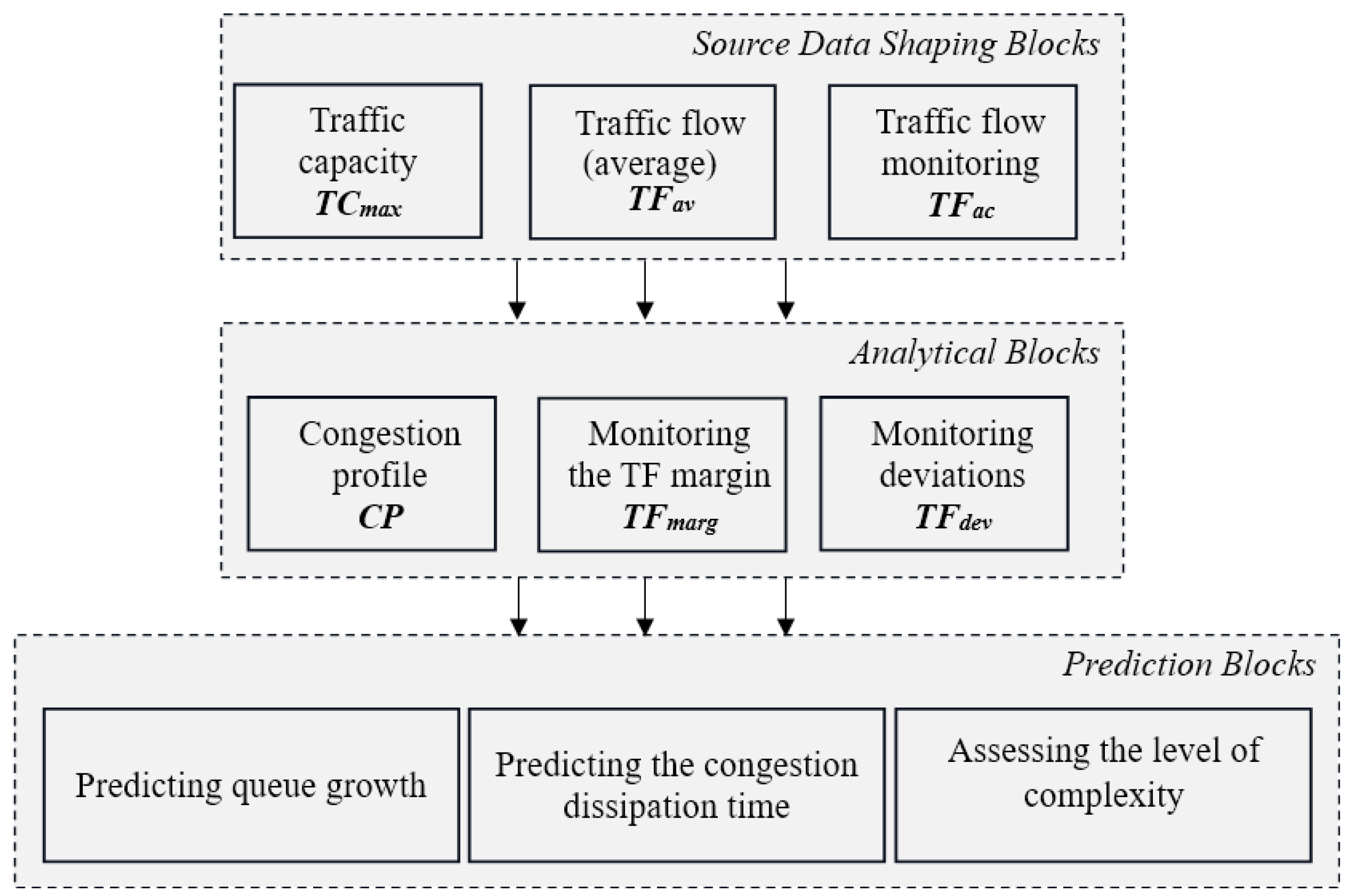
The final result of the developed computer model is the implementation of a software module for the AIMS eco package, designed to predict the aggravating congestion at urban transport network nodes and its dissipation when disturbances are eliminated. This implies the presence of a source data shaping macroblock, a calculation and analytical block for signaling potential congestion, and a traffic congestion state predicting block (Figure 1).

• Source data shaping block.

The source data macroblock, which generally provides information in real time, should include the following blocks:

• A block for determining the saturation flow (SF) or maximum traffic capacity (TC_max), both for the traffic directions and for the crossing intersection as a whole;
• A block for generating the actual hourly average traffic flow (TF_av). We assume that TF_av corresponds to unsaturated traffic;
• A block for monitoring the actual 2 min traffic flow (TF_ac).

2.

Analytical block.

The analytical macroblock should include blocks for calculating deviations in the traffic capacity values for the traffic directions: maximum, average, and actual over an averaged two-minute time interval. Based on these calculations, signal information about the possibility of congestion will be generated. The analytical macroblock will include the following blocks:

• A block for creation of a “congestion profile” (CP) for the intersection as a margin in the deviation of the average capacity of traffic directions from the maximum capacity (CP = TCmax – TCav);
• A signaling block for monitoring the margin based on the actual capacity (TFmarg = TCmax − TFac);
• An analytical block, in the presence of congestion, of the actual traffic flow deviation from the average one (TFdev = TFav − TFac).

3.

Prediction block.

In case of congestion, forecasts are made for the increase in the queue of vehicles, or for the dissipation of the traffic congestion when its cause is eliminated. The levels of capacity deviations identified by the analytical block will be used to assess the level of complexity of a possible traffic congestion. The prediction block will include the following blocks:

• A block for predicting the increase in the queue of vehicles in a traffic congestion;
• A block for predicting the congestion dissipation time after elimination of the cause of congestion;
• A block for assessing the level of complexity of possible congestion.

This paper examines in detail the construction of computer models for the third block, which will subsequently serve as the basis for implementing a similar software block for predicting traffic congestion in the AIMS eco package.

4. Predictive Mathematical Model

Let us consider the basic mathematical relationships that determine the calculated content of the blocks in the predictive part of the conceptual model.

It should be noted that all calculations use the specific value of traffic intensity, determined by the formula:

$$N_{sp}=k_1·N_1+k_2·N_2+\cdots +k_n·N_n,$$

(1)

where k₁, k₂, …, k_n are coefficients for converting vehicle types to passenger car equivalents; N₁, N₂, …, N_n are the number of moving vehicles.

A common approach to create a traffic congestion predictive model that takes into account historical traffic data with a 2 min increment, the number of lanes and their maximum capacity, and the impact of accidents on the capacity of each lane, can be applying the multiple regression, taking into account the dynamic influence of factors. The linear multiple model is represented as follows:

$$\begin{gathered} T_C\left(t\right)=f\left[I\left(t\right);V\left(t\right);N;C;P;S;T\right]= \\ {a}_0+a_1·I\left(t\right)+a_2·V\left(t\right)+a_3·N+a_4·C+a_5·P+a_6·S+a_7·T, \end{gathered}$$

(2)

where T_C is the time it takes for the congestion to reach a certain level; I(t) is traffic density at time t (vehicles/2 min); V(t) is average speed at time t (km/h); N is the number of lanes in the direction at the intersection; C is the maximum capacity of a line (vehicles/2 min); P is the number of lanes closed due to accidents; S is the share in the reduction in capacity for each closed lane; T is time of day (to account for peak hours).

The advantage of this approach is that it identifies the main factors influencing traffic congestion. However, in this form, where all factors are considered equal, the regression model is not correct. Generally, it is necessary to separate time-dependent factors from constant or weakly time-dependent parameters.

More accurately, a congestion situation in one direction at a controlled intersection should be characterized by the number K_C(t) of vehicles causing the congestion, which is dynamic depending on the number of time t increments with generally accepted duration of 2 min. In this case, the dependence of K_C(t) on the stated factors can be explicitly expressed by the formula:

$$\begin{gathered} Kc\left(t\right)=\sum _{i=1}^t\left[TFac\left(i\right)·{\displaystyle \frac{\sum _{j=1}^{P\left(i\right)}{S}_j\left(i\right)}{N}}-\left(TCmax-TFac\left(i\right)\right)·{\displaystyle \frac{\left(N-P\left(i\right)\right)}{N}}\right], \mathrm{i}\mathrm{f} Kc\left(t\right)>0 \\ Kc\left(t\right)=0, \mathrm{i}\mathrm{f} Kc\left(t\right)\le 0 , \end{gathered}$$

(3)

where t is the time changed by given increments of 2 min; TF_ac(i) is the actual crossing capacity in one direction; TC_max is the maximum crossing capacity in one direction; P(i); S_j(i) are the number of lanes closed due to accidents and the share in the reduction in capacity for each closed lane (parameters can change dynamically over time).

The general form of Formula (3) can be simplified by assuming that the cause of congestion is constant over time, and by replacing the actual capacity with its average value over a 2 min period:

$$Kc\left(t\right)={\sum }_{i=1}^t\left[TFav·{\displaystyle \frac{\sum _{j=1}^P{S}_j}{N}}-\left(TCmax-TFav\right)·{\displaystyle \frac{\left(N-P\right)}{N}}\right].$$

(4)

The transition from the general form in Equation (3) to the simplified Equation (4) is justified by the short-term nature of the prediction horizon. Over a 2 min interval, the primary cause of congestion –such as the number of closed lanes (P) and their capacity reduction (S_j)—can be considered constant for the purpose of operational forecasting. This assumption aligns with traffic flow theory, where parameters are often treated as stationary over short durations for manageability and stability in estimation. It allows us to substitute the dynamically changing actual capacity TF_ac(i) with its average value TF_av over the interval, significantly simplifying the model while maintaining forecasting accuracy for the near future.

In this form, Equation (4) can be used to estimate the growth of congestion as the number of vehicles accumulating on the highway in front of the intersection, depending on time.

It is also possible to calculate the queue length growth L(t), based on the dimensions of vehicles D_i of various k classes and their percentage content mi in the traffic flow, as well as the average distance between vehicles in the congestion ∆L:

$$L\left(t\right)=Kc\left(t\right)·{\displaystyle \frac{1}{N}}·\left(∆L+\sum _{i=1}^k\left(D_i·m_i\right)\right).$$

(5)

The predicted time T for the congestion to dissipate can be estimated based on the increase in crossing capacity from the average TF_av to the maximum possible TC_max after eliminating the cause of the congestion. In this case, the time estimate is calculated using the formula:

$$T={\displaystyle \frac{Kc\left(n\right)}{TCmax-TFav}}$$

(6)

where T is the number of 2 min time increments; K_C(n) is the number of vehicles in the congestion at the time its cause is eliminated, calculated using Equation (4).

In the model version, it is advisable to assess the congestion complexity level based on the direction capacity reduction on the intersection where the congestion occurred. In this approach, the congestion complexity score (CS), as a measure of the reduction in capacity, can be determined based on the constants characterizing the congestion, using the formula:

$$CS=1-{\displaystyle \frac{\sum _{j=1}^{P_j}·S_j}{N}}$$

(7)

Based on the expert assessments of the authors, the following classification of traffic congestion complexity levels is proposed, accompanied by a specific value for the CS congestion complexity score calculated parameter:

• Level 1: CS = (0.1–0.3)—light congestion, minor impact on traffic;
• Level 2: CS = (0.3–0.6)—moderate congestion;
• Level 3: CS = (0.6–0.9)—severe congestion, requiring intervention;
• Level 4: CS = (0.9–1)—extreme congestion, requiring an immediate solution.

Let us conduct a preliminary evaluation experiment using the congestion growth model determined by Formula (4) for the eastbound three-lane intersection of Lenin Avenue and Engels Street in Chelyabinsk, Russian Federation. 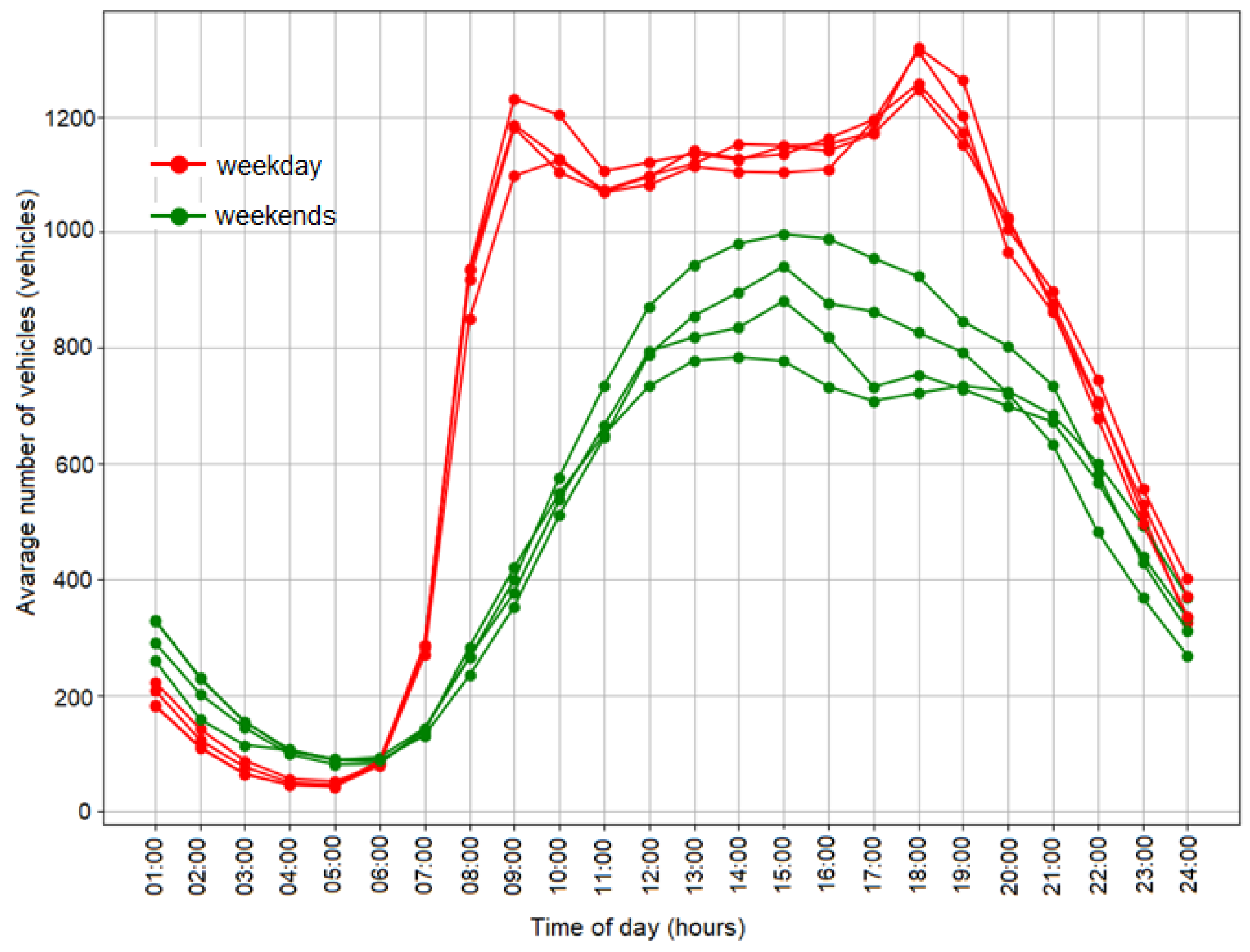The value of the average hourly load TF_av of the traffic flow for June 2024 is determined from the database of the AIMS eco software package https://aims.susu.ru/demo/dashboard/chelyabinsk/city (accessed on 1 Octomber 2025) [29] (Figure 2).

Figure 2 clearly shows the dynamics of traffic flow increase in the morning and evening hours for weekdays and the stability of the flow throughout the month (four average weekly graphs). Days off are characterized by greater flow variations throughout the month and a single average daily peak, which aligns well with a priori expected results.

In the calculations, we assume the actual traffic load level of the TF_av on the highway for 1 July 2024, at 6:00 PM as 1774 vehicles/hour, or 59.1 vehicles/2 min. The maximum capacity TC_max of the highway, according to the AIMS eco software package, is estimated at 2000 vehicles/hour, or 66.7 vehicles/2 min.

For three-lane traffic, Equation (4) takes the form:

$$K\mathrm{c}\left(t\right)=\sum _{i=1}^t\left[59.1·{\displaystyle \frac{\sum _{j=1}^3·S_j}{3}}-7.6·{\displaystyle \frac{3-P}{3}}\right]$$

(8)

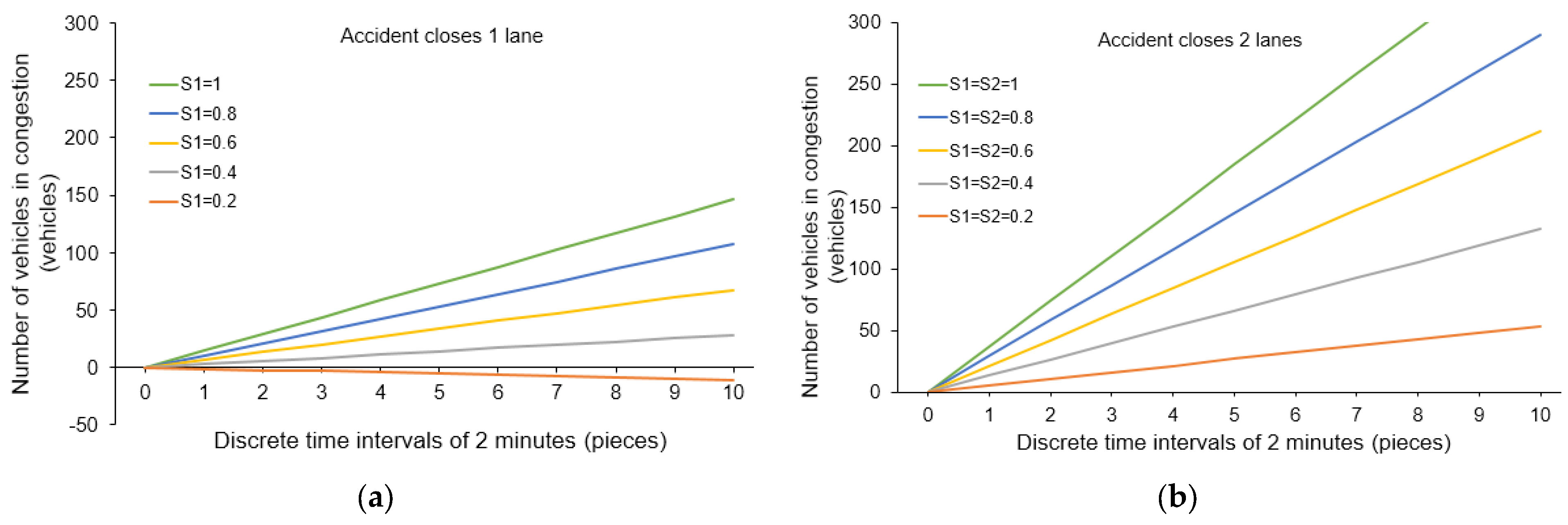
The experiment includes variations in the number of lanes blocked by congestion, as well as the percentage of capacity reduction for each blocked lane. The congestion buildup time t is measured in 2 min increments. Figure 3 shows graphs of the vehicle queue growth in congestion over 10 discrete 2 min increments for different capacity reduction shares of both one and two lanes.

As Figure 3 shows, the growth of the vehicle queue in the congestion is linear. This is due to the simplified model, which assumes a constant actual vehicle flow and the state of the congestion itself.

The congestion growth model can be complicated by taking into account 2 min random variations in the actual traffic flow, which adds a probabilistic element to the model. In this case, the model under consideration turns from the class of continuously deterministic models (D-scheme) to the class of stochastic models (Q-scheme). To introduce probabilistic processes into the congestion growth model under consideration, it is necessary to evaluate the statistical characteristics of the actual traffic flow, such as the characteristics of the center and the variations for the 2 min initial data.

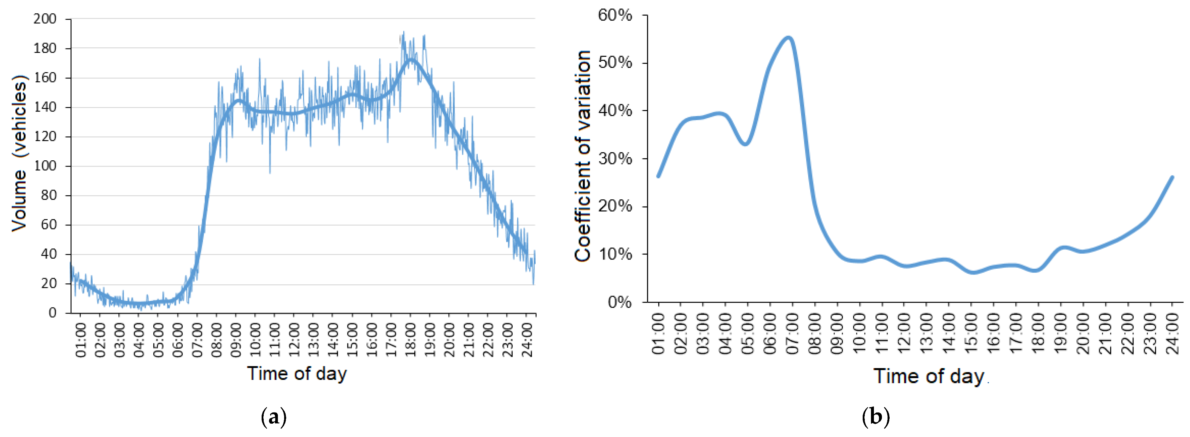
Traffic flow variations over two-minute intervals during one working day were obtained from the AIMS eco software database. Figure 4a presents them against the hourly average values. The figure also demonstrates the change in the mean square deviation of traffic flow for each hour of the day. To enable comparison of these values, the graph shows the variation coefficient, which represents the mean square deviation reduced to the mathematical expectation.

According to Figure 4b, the minimum variations in the number of vehicles are observed during the hours of maximum traffic flow, between 9:00 and 20:00. This time is the most critical for the development of severe traffic congestion. The average variation coefficient in this time range is approximately 10%. The value of this statistical parameter is used as the basis for introducing random factors into the congestion forecast model.

5. Simulation Modeling of Congestion Development

Creating a simulation model of traffic congestion development is most conveniently done using the Matlab mathematical laboratory with the Simulink application. The main advantages of this tool include the ability to record time dependencies of the parameters of interest, as well as the rapid generation of both random variables with specified statistical parameters and dynamic blocks simulating the inertia of real processes.

A general approach to creating a simulation model for studying multi-lane highway traffic congestion involves identifying submodels of the same type for each traffic lane, with separate variations in congestion parameters (P_i; S_i) for them. In the first stage of modeling, a deterministic D-class model is created, which is then complexified to a stochastic Q-model by introducing a random actual flow (TF_ac) with the statistical parameters defined above.

The transition from the deterministic model (D-scheme) to the stochastic model (Q-scheme) is achieved by modeling the actual traffic flow TE_ac(i) as a random variable. The statistical parameters for this variable—the mean (μ), variance (σ²), and coefficient of variation (CV)—are derived directly from the historical 2 min traffic data (see Figure 4). This approach explicitly accounts for the inherent randomness in vehicle arrivals. The key assumption here is the local stationarity of the traffic flow process within each 2 min interval, enabling the use of fixed statistical moments to describe the stochastic dynamics of congestion formation. The core algorithm for this stochastic simulation is summarized in the pseudo-code provided in Appendix A Algorithm A1.

For the three-lane highway discussed above, the mathematical model, defined based on Equation (4), is transformed to the following form:

$$Kc\left(t\right)=\sum _{i=1}^t\left[\sum _{j=1}^3\left({\displaystyle \frac{1}{3}}TFac(i)·P_j·S_j\left(i\right)+\left(TCmax-TFac\left(i\right)\right)·\left(P_j-1\right)\right)\right]$$

(9)

where TF_ac(i) is the actual traffic flow, which can generally change dynamically over time, determined by index i— the two-minute current time increment; the P_j parameter determines whether congestion is present in the j-th lane (P_j = 1) or absent (P_j = 0); the S_j(i) parameter is the share in traffic capacity reduction due to congestion in j-th lane (it can also change dynamically over time).

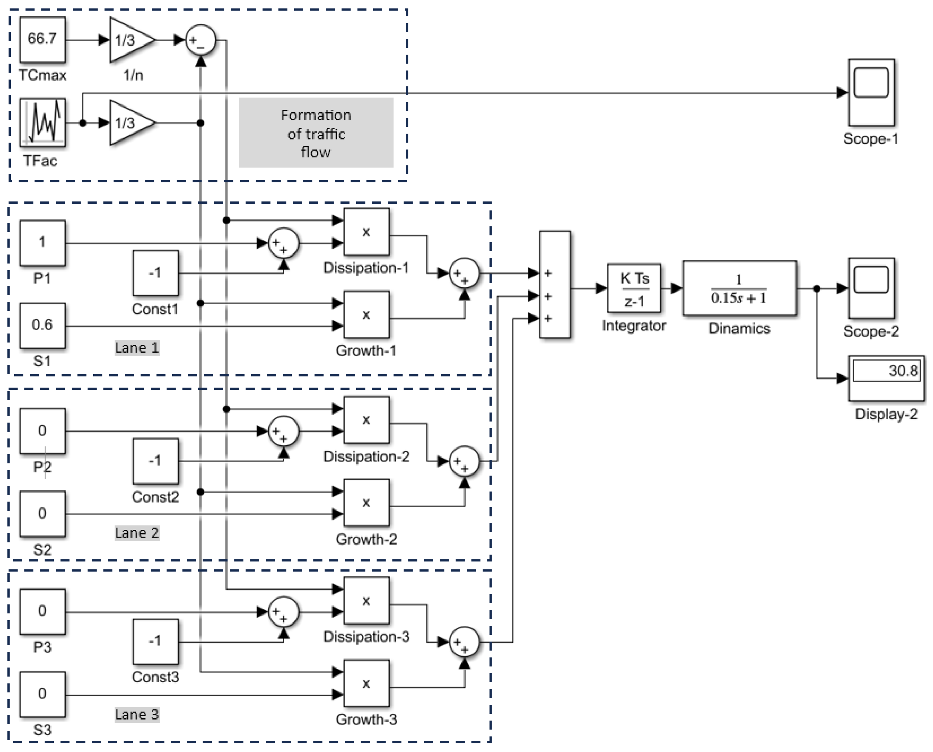
In this case, for each of the three lanes, either the first term from Equation (9) (presence of congestion) or the second one (absence of congestion) is taken into account. The corresponding simulation model is shown in Figure 5.

The presented Q-model of traffic congestion formation includes autonomous blocks for increasing the number of vehicles in each of the three lanes, which are determined individually by the input stationary congestion parameters (P_j; S_j). A discrete integrator allows for the summation of vehicles in the congestion over time for two-minute traffic light cycles. A common inertial “Dynamics” block, simulating the actual process of vehicle queue growth, has also been added to the model.

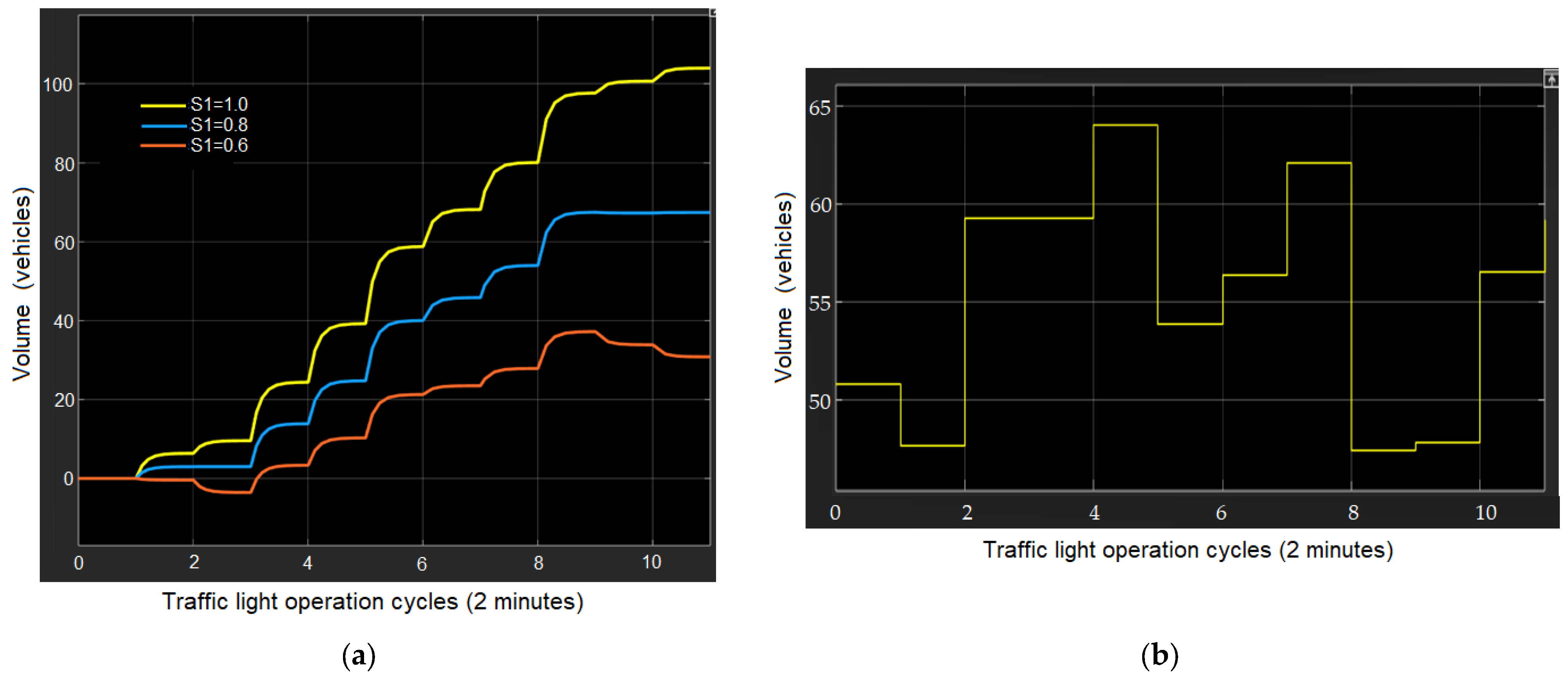
The experimental studies are focused on similar initial data expressed in Equation (7) for the eastbound highway at the selected intersection. Figure 6a shows the graph of the increase in congestion during an accident on the first lane, which restricts traffic by 100%, 80%, and 60%, over 10 standard 2 min traffic signal cycles.

Figure 6a clearly demonstrates the discreteness and dynamics of the vehicle queue growth in the congestion, as well as the random nature of the queue size change over time. Moreover, as the share S_j in traffic capacity reduction decreases, the congestion may not increase, but even resolve.

It should be noted that the statistical parameters of the actual TF_ac flow were determined for the time period of 18:00–19:00 (maximum traffic flow) and are as follows: mean value m_x = 59.1 vehicles/2 min; variation coefficient K_var = 6.7%. Figure 6b shows the time realization of a random TF_ac signal with a uniform distribution in the conventional variation range (m_x ± 3∙σ).

The conducted experiment demonstrates the general trend of vehicle queue formation in congestion over a short-term time scale. The dynamics of congestion over a time scale of several hours, when the traffic situation is unstable, are also of interest, in particular, with the change in the actual traffic flow TF_ac = f(t) over time. For this purpose, another experiment was developed and conducted: a dynamic reduction in the TF_ac parameter was implemented for a time range starting with the peak flow at 6:00 PM over a period of 3–4 h.

Figure 7 shows a graph of the actual traffic flow for the eastbound highway at the intersection under study for 120 two-minute time increments (4 h). It clearly demonstrates a steady downward trend in the TF_ac parameter.

The simplest linear trend to implement in the model, also shown in Figure 7, has a high approximation quality (R²), covering 84.82% of the actual traffic flow variability.

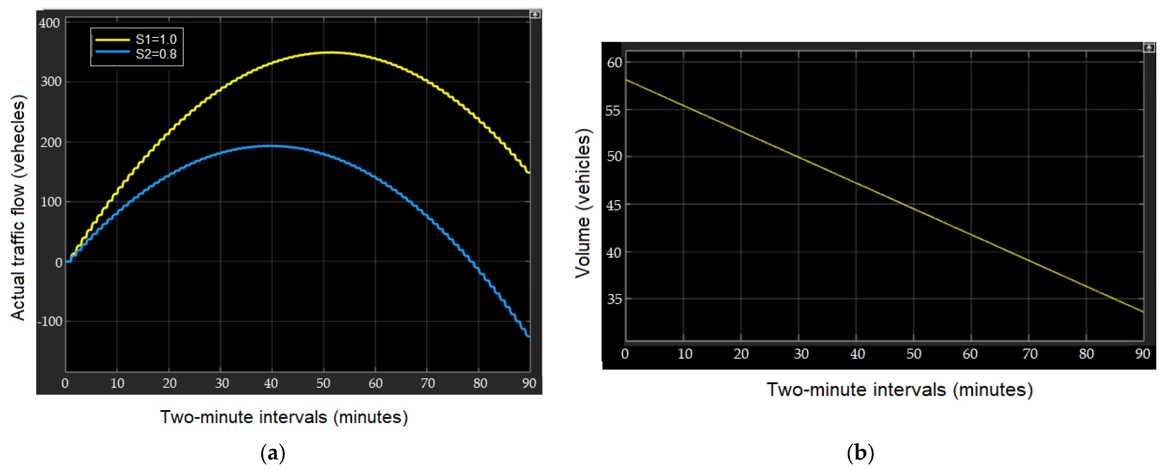
The revealed linear time dependence model, TF_ac(t) = 58.14 − 0.2726 × t, is implemented in a simulation model without stochastic variations. The experimental results for a three-hour time range starting at 6:00 PM (90 two-minute increments) are shown in Figure 8.

As follows from the oscillogram in Figure 8a, when the actual traffic flow TF_ac decreases (Figure 8b), the congestion tends to dissolve on its own, even without any possible regulatory measures, such as eliminating the cause of the congestion or redirecting traffic flows to other routes. For example, when the capacity is reduced from S1 = 1 to S1 = 0.8, the congestion completely disappears in approximately 2.5 h. This is followed by a “flow growth reserve” defined by negative values for the queue size of vehicles in the congestion.

Subsequent simulation experiments involve the consideration and analysis of congestion of increased complexity (2 or 3 lanes with varying degrees of capacity reduction), as well as longer-term congestion, in which the statistical parameters of the actual traffic flow (TF_ac) change over time in accordance with Figure 2 or Figure 4.

In general, the presented simulation model serves as an illustrative simulator for analyzing congestion of varying complexity. Various model experiments identify general trends in the dynamics of vehicle congestion at various levels of complexity.

This will be a good basis for the subsequent creation of a corresponding predictive block in the AIMS eco software package [29] to develop informed management decisions to reduce the impact of congestion on the operation of the urban transport network.

6. Queue Length Prediction

6.1. Problem Statement and Data Preparation

To implement the predictive module in the AIMS eco system, the problem stated was the short-term prediction of key congestion parameters. A deep learning model operating on time series was chosen due to its ability to detect complex nonlinear relationships in sequential data.

The input data was obtained from the AIMS eco database and included records of vehicles passing through a selected intersection in Chelyabinsk over a period of seven working days. To standardize different type vehicles, conversion factors for passenger cars were used (Reduced number of vehicles = 1.0 × car + 3.0 × trolleybus + …). Trams were excluded from the analysis since their movement is often isolated from the general traffic flow. After processing, a time series of 138,663 records with two-minute increments was formed.

The maximum observed direction capacity over 2 min was 60 vehicles. This parameter was used to normalize the input data. Each input sample for the model represented a 1 h sequence (30 time intervals) and consisted of two features:

• Normalized number of vehicles per interval (from 0 to 1);
• Normalized time of day (from 0 to 1, where 1 corresponds to 1440 min).

Figure 9 represents the proposed neural network configuration.

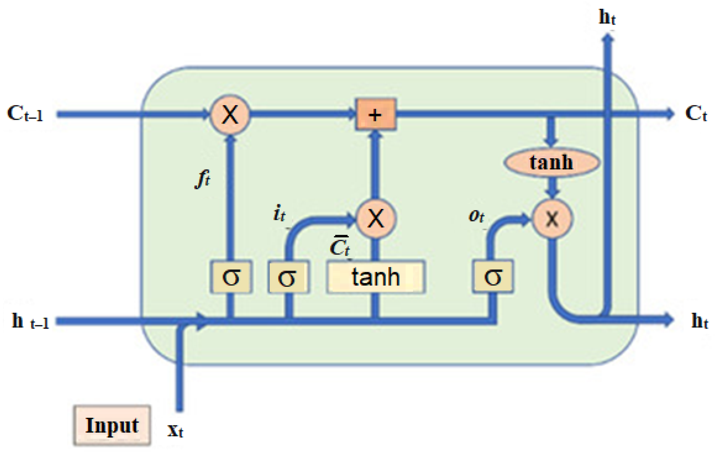
A LSTM neural network architecture is given in Figure 10 [55].

Here, x_t represents the observation of a vehicle at time t. C_t is the memory cell, which contains the information at time step t; σ indicates the sigmoid function, f_t is the output of the Forget gate at time t.

6.2. Hybrid Neural Network Architecture

A number of architectures were developed and tested for predicting. The best results were achieved by a hybrid model combining convolutional layers (CNN), long short-term memory (LSTM) layers, and an attention mechanism (Transformer). The motivation for choosing this architecture was as follows:

• Convolutional layer (CNN): Reveals local patterns and short-term dependencies in the data (e.g., traffic fluctuations over a period of a few minutes).
• LSTM layer: Captures long-term time dependencies and cyclic patterns (e.g., morning and evening peak hours).
• Attention mechanism (Transformer): Allows the model to dynamically “weight” the importance of different instants of time in the input sequence, which is critical for predicting abnormal events such as congestion.

The model output is a vector of three parameters for 20 increments ahead (40 min):

• Queue Growth: the number of vehicles that failed to pass the intersection during the interval and increased the queue;
• Total Queue Size: the total number of vehicles in the queue at the end of the interval;
• Lane Closure Percentage: an exogenous parameter modeling the impact of accidents or road works.

The original dataset contained 138,663 records. It included data of 7 working days, one direction of vehicle movements. Brief statistics of the initial data is given in

Table 1. Statistics of the initial dataset.

Number of Samples, Records	Total Vehicle Number of All Types, mln	Sampling Period
138,663	~0.56	1 April 2025, 2 April 2025, 8 April 2025, 9 April 2025, 14 April 2025, 22 April 2025, 30 April 2025

.

It was expanded artificially by overlapping bands from 0% to 100% with no use of generative algorithms or noise augmentation (10):

$${Count}_{new}={Count}_{current}\times P-\left({Count}_{max}-{Count}_{current}\right)\times (1.0-P)$$

(10)

where P is the overlap of the road from 0 to 1; current_count and max_count are the current and maximum number of people who have passed the intersection over the entire time. Thus, the volume amounted to ~14 million records and covers various load and lane overlap scenarios.

6.3. Model Comparison

The following neural network models were selected for comparison:

• LSTM Full (LSTM + CNN + Attention, which is our proposed hybrid model)—a com-plete model with CNN preprocessing, normalization, two-layer LSTM and attention mechanism;
• LSTM Only—a simplified version using only two LSTM layers without additional modules;
• LSTM + CNN—a model with a convolutional layer in front of the LSTM to highlight local time patterns;
• LSTM + Attention—a model that uses Multi-Head Attention after LSTM to account for long-term dependencies;
• LSTM Full (20-Step Input)—a complete model, but with a shortened input history to assess the impact of input length;
• BiLSTM—a bidirectional LSTM that processes the forward and backward sequence;
• GRU—a simpler and lighter alternative to LSTM;
• BiGRU—a bidirectional version of GRU to account for the reverse context;
• TransformerEncoder—a simplified transformer encoder that uses only attention mechanisms without recurrence.

Due to limited resources, only a part of the dataset was taken, around 5,000,000 ran-dom records. The resulting dataset was divided into training/validation/test parts in the ratio of 80%/10%/10%. The training and testing were performed on an NVIDIA A30 graphics card. The model was trained with the adam optimizer (learning rate = 0.0001) and the MSE loss function. Early Stopping (patience equal to 5; restoring the best weights) and ReduceLROnPlateau (reducing the learning rate by two times in the absence of im-provements) were used for stabilization. The training was performed for up to 100 epochs with batch size = 1024, and validation on a separate set. The training of each model lasted about 2 h. The comparison results for MAE, RMSE (denormalized by the first and second parameters, and as a percentage by the third), the inference time, and the number of parameters are shown in

Table 2. Results of comparing neural network models by MAE, RMSE, inference time, and number of parameters.

Model	Queue Growth		Total Queue Length, Vehicles		Percentage of Overlap, %		Inference Time, ms	Parameters
	MAE	RMSE	MAE	RMSE	MAE	RMSE
LSTM Full (proposed)	1.72	3.35	0.31	0.70	10.08	16.51	8.43	880,700
LSTM Only	1.84	3.49	0.40	0.81	10.80	16.99	4.95	486,588
LSTM + CNN	1.74	3.36	0.31	0.70	10.42	16.77	4.80	617,020
LSTM + Attention	1.80	3.45	0.37	0.77	10.30	16.74	5.80	750,268
LSTM Full (20-Step Input)	1.81	3.47	0.42	0.88	10.54	16.87	5.52	880,700
BiLSTM	1.92	3.58	0.45	0.88	11.77	17.72	6.18	355,516
GRU	1.84	3.50	0.40	0.81	10.73	17.02	4.51	372,156
BiGRU	1.86	3.53	0.42	0.85	10.97	17.20	5.58	273,852
Transformer-Encoder	1.93	3.59	0.45	0.89	11.71	17.77	3.09	157,116

. The result of comparing neural network models by SMAPE (average of 3 parameters), MAE, and RMSE (average of 3 parameters) for short and long horizon (the first and last 5 steps) are shown in

Table 3. Result of comparing SMAPE, MAE, and RMSE metrics of neural network models over a short and long horizon (the first and last 5 steps).

Model	SMAPE	MAE_Short	RMSE_Short	MAE_Long	RMSE_Long
LSTM Full (proposed)	48.13	0.0442	0.0758	0.0458	0.0792
LSTM Only	48.94	0.0476	0.0789	0.0495	0.0822
LSTM + CNN	48.41	0.0454	0.0768	0.0470	0.0802
LSTM + Attention	48.61	0.0456	0.0776	0.0473	0.0809
LSTM Full (20-Step Input)	48.76	0.0466	0.0789	0.0484	0.0819
BiLSTM	49.77	0.0514	0.0821	0.0535	0.0856
GRU	48.95	0.0474	0.0790	0.0492	0.0824
BiGRU	49.27	0.0483	0.0800	0.0503	0.0834
Transformer-Encoder	49.64	0.0513	0.0823	0.0534	0.0859

. The results of comparing neural network models by Error variance, MAE/RMSE (high/low-load) (average of 3 pa-rameters) are shown in

Table 4. Results of comparing neural network models by Error variance, MAE/RMSE (high-/low-load).

Model	Error Variance	MAE (High-Load)	RMSE (High-Load)	MAE (Low-Load)	RMSE (Low-Load)
LSTM Full (proposed)	0.0065	0.0251	0.0421	0.0450	0.1011
LSTM Only	0.0066	0.0270	0.0439	0.0486	0.1042
LSTM + CNN	0.0066	0.0252	0.0419	0.0462	0.1025
LSTM + Attention	0.0067	0.0265	0.0427	0.0465	0.1027
LSTM Full (20-Step Input)	0.0067	0.0319	0.0483	0.0476	0.1035
BiLSTM	0.0067	0.0290	0.0446	0.0525	0.1085
GRU	0.0067	0.0295	0.0453	0.0483	0.1044
BiGRU	0.0067	0.0292	0.0450	0.0493	0.1055
Transformer-Encoder	0.0069	0.0329	0.0496	0.0524	0.1088

.

A comparison of architectures showed that the extended LSTM Full (CNN + LSTM + Attention) model (the proposed one) demonstrates the best accuracy among all tested var-iants. Adding a convolutional block and an attention mechanism allows the model to capture both local and global dependencies well. The LSTM + CNN model shows compa-rable results for the main part of the metrics and is the second in quality: convolution ef-fectively highlights local time patterns and provides a noticeable improvement over the LSTM Only model. The LSTM + Attention variant also improves accuracy relative to the basic LSTM, but is inferior to the CNN architecture, which confirms the great importance of local dependencies in the data. The LSTM Only model shows the worst error values among LSTM-based models, which confirms the need for additional feature extraction mechanisms. The shortened LSTM Full (20-Step Input) model shows a deterioration in all metrics, which confirms the need to use a longer entry history.

GRU and BiGRU show results close to LSTM Only. BiLSTM does not provide an advantage. The TransformerEncoder model demonstrates the worst accuracy among all variants.

The overall result shows the best quality achieved by architectures that combine CNN and LSTM, whereas using attention and transformers without convolutional or recurrent components does not provide an advantage on short time windows.

SMAPE repeats the general trend from Table 1: hybrid models produce the best results. The long horizon hardly worsens compared to the short one.

LSTM Full (proposed) provides the lowest error in both high-load and low-load road conditions. The LSTM + CNN architecture demonstrates comparable quality and in some places surpasses RMSE in high-load modes, but on average, it is slightly inferior to the proposed model. The simplified LSTM Only model is noticeably weaker. The BiLSTM, GRU, and BiGRU models occupy an intermediate position and do not provide advantages. Transformer Encoder shows the worst results in all scenarios. Error variance is almost the same for all models, which indicates the stability of the error and the dominant influence of the task itself, rather than the choice of architecture.

The MAE, RMSE, and error variances for each step for the LSTM Full model are shown in

Table 5. MAE, RMSE, and error variances for each step for the proposed LSTM Full model.

Prediction Step	MAE	RMSE	Error Variance
1	0.044068	0.100677	0.008194
2	0.044066	0.100586	0.008176
3	0.044159	0.100618	0.008174
4	0.044233	0.100648	0.008174
5	0.044296	0.100645	0.008167
6	0.044386	0.100647	0.00816
7	0.044523	0.100676	0.008153
8	0.044612	0.100726	0.008156
9	0.044754	0.10077	0.008152
10	0.04479	0.100812	0.008157
11	0.044903	0.100862	0.008157
12	0.045003	0.10086	0.008147
13	0.045098	0.100898	0.008147
14	0.045123	0.100879	0.008141
15	0.045234	0.100949	0.008145
16	0.045494	0.101031	0.008138
17	0.045592	0.10113	0.008149
18	0.045689	0.101168	0.008147
19	0.045902	0.101267	0.008148
20	0.046098	0.101446	0.008166

The best (minimum) MAE value in the column is highlighted in bold.

.

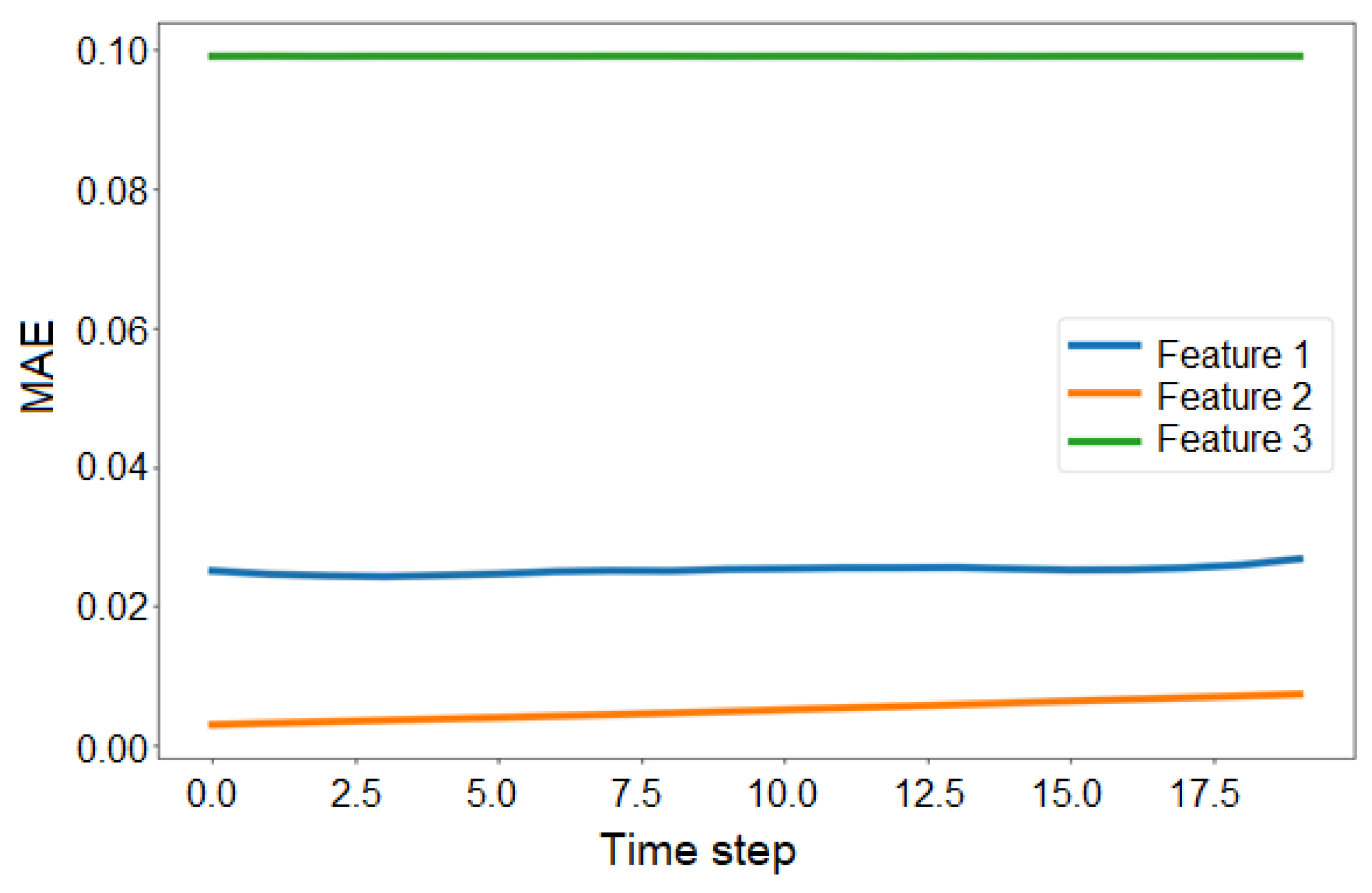
The error in the prediction steps increases smoothly, without jumps and without acceleration. MAE grows from 0.044 to 0.046, RMSE increases from 0.1007 to 0.1014, and the error variance remains almost unchanged. This indicates the high stability of the model and the absence of error accumulation as the prediction horizon increases.

6.4. Model Training and Validation Results

The model was trained for 180 epochs until convergence. Results on the test set (20% of the data) demonstrated high forecast accuracy:

• For queue growth: MAE = 1.5 VE (vehicles), RMSE = 3.1 VE.
• For total queue size: MAE = 0.3 VE, RMSE = 0.7 VE.
• For closure percentage: MAE = 9.9%, RMSE = 16.2%.

Error distribution for all predicted features across the entire validation set is stable, as confirmed by low and converging MAE and RMSE values (Figure 11 and Figure 12).

Interpretation of Results: The MAE value of 0.3 VE for total queue size indicates that, on average, the model error is less than one vehicle when estimating the current congestion length. This is an exceptionally high result for traffic predicting tasks, which validates the model applicability for operational control. The low queue growth error (MAE = 1.5 VE) allows for highly accurate predictions of congestion dynamics 40 min in advance, which is sufficient time horizon for proactive measures (e.g., traffic signal mode correction).

Visual analysis of random samples from the test set (Figure 13) confirms that the model adequately tracks both smooth changes and sharp spikes in the data, indicating its robustness and generalization ability.

7. Discussion

The study demonstrates the efficacy of an integrated approach combining deterministic simulation modeling and deep learning for traffic congestion prediction. A comparative analysis of the results from the Simulink simulation model and the LSTM network reveals a significant synergistic effect from their combined application. The simulation model, which integrates real-time monitoring data, provides a profound understanding of the physical processes underlying congestion formation and dissipation, effectively serving as a digital twin of an intersection. Its key advantage lies in the ability to simulate not only congestion growth but also its natural dissipation as traffic demand decreases or partial obstructions are removed. This capability accurately reflects the nonlinear dynamics of transportation systems and offers a valuable tool for analyzing network resilience.

The high predictive accuracy achieved by the LSTM model, particularly the low error in determining the total queue length (MAE = 0.3 VE), is crucial for practical implementation in ITS. This level of accuracy means the system can monitor traffic conditions with an error of less than one vehicle, establishing a reliable foundation for automated decision-making. For instance, by accurately predicting both the current queue length and its projected growth 40 min in advance (MAE = 1.5 vehicles), the control system can transition from a reactive to a proactive operational mode. This enables not just a reaction to existing congestion, but also the proactive optimization of traffic signal cycles at adjacent intersections or dynamic traffic rerouting, thereby preventing congestion escalation. The stable error distribution for all predicted parameters, as shown in Figure 11 and Figure 12, confirms the model’s reliability and its readiness for integration into decision-support systems such as AIMS eco.

Despite the promising results, this study has several limitations. Although the simulation model incorporates a stochastic component, it operates with largely deterministic congestion parameters (e.g., P_j, S_j). In a real urban environment, these parameters are subject to random variations. Furthermore, the model was validated on data from a limited number of intersections. Its scalability to a city-wide network requires further verification and must account for more complex spatiotemporal correlations between different network nodes.

Future research will be directed along several paths. The primary direction involves creating a unified framework in which the simulation model generates synthetic data. This data will be used to train and stress-test LSTM networks, particularly for scenarios with scarce real-world data on rare but critical congestion events. The integration of additional exogenous factors—such as detailed weather conditions, scheduled roadworks, and public events that significantly alter traffic patterns—is also a priority. Secondly, the development of more sophisticated hybrid architectures is warranted. For example, employing Graph Neural Networks (GNNs) would explicitly model the topology of the road network, capturing the complex interdependencies between intersections.

The implementation of these proposed advancements will contribute to developing a more sustainable, safe, and ecologically friendly urban transport environment. This progress will help reduce the economic and social costs associated with traffic congestion and directly support the achievement of Sustainable Development Goals related to intelligent transportation systems.

8. Conclusions

Currently, research aimed at developing comprehensive approaches combining simulation modeling methods and artificial intelligence for predicting traffic congestion becomes increasingly relevant. The integration of deterministic and stochastic models with deep learning capabilities is a promising direction, taking into account both the physical patterns of traffic flows and the complex nonlinear dependencies identified by neural networks.

This study demonstrates the effectiveness of integrating simulation modeling methods and deep machine learning for solving the challenging task of predicting traffic congestion. The developed comprehensive approach, which uses the capabilities of Matlab Simulink and LSTM networks, allows for highly accurate analysis and dynamics prediction of the congestion of various complexity based on real-time monitoring data of traffic flows.

The practical value of the research is confirmed by the creation of highly accurate predictive models with low error rates (MAE = 0.3–1.5 VE) and the possibility of their integration into software systems such as AIMS eco. The developed solutions form the basis for passing from reactive to proactive traffic management.

Areas of further research may include improving the proposed hybrid architecture of the model, for example, combining it with graph neural networks to improve performance, or developing federal models to more accurately account for spatial and temporal dependencies in traffic data, reduce network traffic, and increase the overall security of sensitive data. Additionally, it will be possible to add new data ranges and design a multimodal model to include new data sources (GPS tracks, data from traffic sensors, weather conditions, cameras, social networks, lidars, etc.) and explore various mechanisms for merging modalities. An explanation of how the models work is becoming highly demanded, including for the traffic congestion prediction model, the results of which will be used by administrative decision makers.

The issue of processing anomalies and their impact on the formation of local or net-work congestion (accidents, road works, mass events, road cleaning with special equipment, etc.) remains insufficiently investigated.

Horizontally, further research may cover issues of integration with real-time traffic control systems: using congestion duration predictions for adaptive traffic light control.

The practical application of the predicting system can be reflected in decision support and early warning systems: for example, the creation of panels for dispatchers with fore-casts and confidence levels, notifications of potential long-term congestion and recommendations for routing public transport, special equipment, and emergency rescue teams.

An important consequence of the expansion of the practical application of the pro-posed model may be more optimal planning and assessment of the effect of infrastructural changes (the introduction of new lanes, changing priorities of public transport), which may increase the planning horizon for the sustainability of modern cities.

Implementation of the presented developments will contribute to the creation of a more sustainable, safe, and ecologically friendly urban transport environment, reducing the economic and social costs associated with traffic congestions.

The developed model enables a transition from reactive to proactive management in intelligent transportation systems such as AIMS eco. The high-precision forecast of queue dynamics (MAE = 0.3–1.5 vehicles) with a 40 min prediction horizon allows the system to not just detect emerging congestion, but to proactively initiate preemptive scenarios: adaptively reconfigure traffic light cycles at neighboring intersections and redirect traffic flows. This prevents the avalanche-like growth of traffic congestions, implementing the principle of proactive control fundamental to modern intelligent transportation systems.