Article

Diffusion-Driven Time-Series Forecasting to Support Sustainable River Ecosystems and SDG-Aligned Water-Resource Governance in Thailand

by
Weenuttagant Rattanatheerawon
and
Rerkchai Fooprateepsiri
*
Institute of Innovation Lifelong Learning, Rajamangala University of Technology Tawan-ok, Chonburi 20110, Thailand
*
Author to whom correspondence should be addressed.
Sustainability 2025, 17(22), 10295; https://doi.org/10.3390/su172210295
Submission received: 28 September 2025 / Revised: 11 November 2025 / Accepted: 12 November 2025 / Published: 18 November 2025

Abstract

Time-series water-quality forecasting plays a crucial role in sustainable environmental monitoring, early-warning surveillance, and data-driven water-resource governance. Degradation of river ecosystems poses significant risks to public health, biodiversity, and long-term socio-economic resilience, particularly in rapidly developing regions. In this study, a multi-scale diffusion forecaster (MDF) is introduced to enhance predictive accuracy and uncertainty quantification for river water-quality dynamics in Thailand. The proposed framework integrates seasonal-trend decomposition with a hierarchical denoising diffusion process to model stochastic environmental fluctuations across multiple temporal resolutions. Experiments conducted using real water-quality datasets from the Mae Klong, Khwae Noi, and Khwae Yai Rivers, and the Port Authority of Thailand, demonstrate that MDF achieves superior probabilistic calibration under noise and data incompleteness compared to conventional deterministic baselines. The forecasting capability supports proactive pollution control, sustainable resource allocation, and climate-resilient water-policy design, directly contributing to Sustainable Development Goals (SDG 6: Clean Water and Sanitation; SDG 13: Climate Action; and SDG 14: Life Below Water). The findings highlight the potential of diffusion-based learning as an enabling technology for sustainable aquatic ecosystem governance and long-term environmental planning.

1. Introduction

Clean and resilient water systems are fundamental pillars of sustainable development, ecological conservation, and public health protection. River basins supply drinking water, support agricultural production, maintain aquatic biodiversity, and serve as socio-economic lifelines for communities. However, rapid urbanization, industrial discharge, agricultural runoff, and climate-driven hydrological volatility intensify the vulnerability of water resources in developing regions, including Thailand. Sustainable water-quality monitoring and predictive modeling are therefore essential to support proactive management, pollution-mitigation strategies, and compliance with international sustainability frameworks such as the United Nations Sustainable Development Goals (SDG 6: Clean Water and Sanitation; SDG 13: Climate Action). In this context, advanced forecasting tools capable of handling incomplete, noisy, and non-stationary time-series data play a vital role in ensuring early detection of ecological threats and enabling long-term planning for river ecosystem protection.
Despite their importance, real-world time series [1,2,3,4] often contain missing values, irregular sampling, and noise, arising from sensor failures or communication errors. These imperfections hinder conventional learning algorithms that assume continuity and stationarity. Two main research directions have been emphasized: imputation, to reconstruct missing values, and forecasting, to predict future trajectories. Recent advances in generative artificial intelligence (AI)—notably diffusion probabilistic models—have offered promising solutions by learning to approximate complex temporal distributions through iterative denoising. However, current diffusion-based [5,6,7,8] forecasters generally treat sequences as single-scale signals and thus neglect hierarchical temporal dependencies that occur simultaneously at seasonal, trend, and local levels. Moreover, they show limited robustness to non-Gaussian disturbances and high uncertainty.
Diffusion models have been successfully applied to both imputation and forecasting tasks, and their performance has often exceeded that of generative adversarial networks (GANs) and variational autoencoders (VAEs) [9,10,11]. Building upon these advantages, the present study conducts a comprehensive investigation of diffusion models in the context of real-world case studies of water-quality monitoring in the Mae-Klong, Khwae-Noi, and Khwae-Yai Rivers, Thailand [12]. The challenges of imputation and forecasting under conditions of limited and incomplete data are specifically highlighted. To overcome these challenges, this paper proposes a multi-scale diffusion forecaster (MDF) that integrates seasonal-trend decomposition with a hierarchical conditional denoising process. MDF captures temporal dependencies from coarse-to-fine scales, enabling progressive refinement of forecasts under uncertainty. The main contributions are as follows:
(1)
A multi-scale diffusion architecture that jointly models coarse and fine temporal structures for improved representational fidelity.
(2)
A progressive denoising mechanism guided by coarse-level trends, enhancing stability against noise.
(3)
A comprehensive empirical evaluation comparing MDF with both deterministic and diffusion-based baselines.
(4)
A fully reproducible implementation, with open-source code, including multi-scale trend extraction, forward/reverse diffusion, conditioning networks, and inference modules.

2. Preliminaries

Diffusion Probabilistic Models

The concept of the diffusion model was initially introduced by Sohl-Dickstein et al. [8] and subsequently refined by Ho et al. [5] through the application of variational inference. A diffusion model is structured into two principal phases: the forward process and the reverse process. The forward process gradually perturbs the original data by adding noise in an iterative manner until the data are transformed into pure Gaussian noise. Conversely, the reverse process aims to restore the original data distribution by training a neural network to iteratively denoise the noisy samples. The overall framework of these processes is illustrated in Figure 1.
(1) Forward Process:
Let X 0 R M × N represent the original input matrix, where the superscript 0 denotes the initial state before the introduction of noise. The sequence of progressively noisier states is expressed as X 1 , X 2 , . . . ,   X K . The forward process of the diffusion model is represented as defined as follows:
q ( X K | X K 1 ) = N ( X K ; α k X K 1 , ( 1 α k ) I )
where α k for k = 1 , 2 , K are hyperparameters that control the magnitude of noise injected at each step. After a sufficient number of iterations, X K converges to a sample from a standard Gaussian distribution N ( 0 , I ) .
This formulation is represented as equivalently expressed to represent the cumulative effect of the noising process from X 0 to X K . As derived in [8], the resulting closed-form distribution is given by the following:
q ( X K | X 0 ) = N ( X K ; α k ~ X 0 , ( 1 α k ~ ) I )
where α k ~ : = i = 1 k α i denotes the cumulative product of the noise schedule up to step k .
(2) Reverse Process:
The reverse process is defined as the generative phase, in which the model reconstructs X 0 from noisy observations X K . This process is governed by a neural network through parameterization with learnable parameters θ , and is formulated as follows:
p 0 X k 1 X k = N X k 1 ; μ θ ( X k , k ) , Σ θ ( X k , k )
The training objective, introduced by Ho et al. [5], simplifies the variational lower bound into a denoising score-matching loss, which enables the network to estimate the noise introduced throughout the forward process. Specifically, a noisy sample is represented as reparameterized from Equation (2) as follows:
X k = α k ~ X 0 + 1 α k ~ ϵ , ϵ ~ N ( 0 , I )
The loss function proposed in [5] is expressed as follows:
L s i m p l e θ = E X 0 , ϵ , k ϵ ϵ 0 X k , k 2
where ϵ 0 X k , k denotes the predicted noise at timestep k obtained through the neural network, commonly implemented as a U-Net or transformer. During training, the objective is to minimize the error arising from the discrepancy between the predicted outcomes and the actual target values and the true Gaussian noise ϵ . In achieving this, the network learns to approximate the noise distribution imposed during the forward process.
Once training is complete, the estimated noise ϵ 0 X k , k is represented as employed to recover X 0 from noisy observations X k . This iterative denoising procedure enables the diffusion model to approximate the true data distribution by modeling the reverse stochastic process. Consequently, the trained diffusion model is capable of generating synthetic samples by initiating Gaussian noise and progressively denoising. Such models can, therefore, be applied effectively to both time-series forecasting and imputation tasks in scenarios with incomplete or limited data [3,13].

3. Related Works

In recent years, a wide range of deep learning models for time-series analysis have been introduced, with particular emphasis on transformer-based approaches [14] for capturing temporal dependencies. Informer [15] enhanced the original transformer by mitigating its quadratic computational complexity through sparse attention, while also accelerating inference by employing a non-autoregressive decoding strategy. Autoformer [16] replaced the conventional self-attention mechanism with an auto-correlation layer. Fedformer [17] incorporated a frequency-enhanced module to extract temporal structures via frequency-domain mapping. Similarly, Pyraformer [18] introduced a pyramidal attention module to provide a multi-degree of refinement representations of temporal signals. Scaleformer [19] adopted a progressive forecasting strategy, generating coarse-level predictions initially and refining them sequentially at finer scales. PatchTST [20], inspired by the Vision Transformer (ViT) [21], advanced time-series forecasting by segmenting sequences into patches and applying self-supervised pre-training to extract semantic features. Furthermore, it replaced the transformer’s decoder with a linear mapping and employed a channel-independence strategy, thereby achieving notable performance in multivariate forecasting tasks.
In addition to transformer-based models, basis expansion methods have also been utilized for time-series modeling. FiLM [22] projected historical data onto Legendre polynomials for approximation, while Fourier projections were employed for noise reduction. N-BEATS [23] parameterized long-term trends through polynomial coefficients and seasonal components via Fourier series. DEPTS [24] extended this framework by integrating a periodicity module to improve performance on periodic data. N-HiTS [25] further advanced N-BEATS by incorporating multi-scale hierarchical interpolation. These basis expansion models are generally considered easier to train compared to transformer variants, although their performance is sensitive to the choice of basis functions. Beyond these categories, several alternative architectures have demonstrated competitive performance. SCINet [10] exploited a recursive downsampling–convolution–interaction architecture designed to extract temporal features from subsampled inputs. NLinear [26] applied normalization to the time series before utilizing a linear transformation layer for prediction, while DLinear [26] incorporated seasonal-trend decomposition in a manner analogous to Autoformer.
More recently, diffusion-based approaches have been explored for time-series applications. TimeGrad [27] adopted a conditional diffusion framework guided by recurrent neural network hidden states, though its autoregressive decoding resulted in computational inefficiency for long sequences. To address this limitation, Tashiro et al. [28] presented CSDI for utilizing non-autoregressive generation with self-supervised masking, albeit at the cost of employing two transformers, thus retaining quadratic complexity. The masking-based conditioning also introduced discontinuities at the boundaries between observed and imputed regions [29,30]. This issue persisted in SSSD [13], which replaced transformers with structured state-space models but maintained the same masking strategy. To alleviate boundary inconsistencies, TimeDiff [30] employed autoregressive initialization and future mixup as conditioning mechanisms. Nonetheless, existing diffusion models have not fully exploited multi-degree of refinement temporal structures and typically commence denoising from random noise, as in standard diffusion formulations. To overcome these shortcomings, a decomposition of time series into multiple resolutions through seasonal-trend decomposition is proposed in this work. Fine-to-coarse trends are subsequently utilized as intermediate latent variables to guide the denoising process. Moreover, recent efforts have explored alternative multi-degree of refinement analysis frameworks beyond seasonal-trend decomposition. For instance, Bui [31] employed a U-Net [32] for graph-structured temporal data, leveraging pooled features across resolutions. Mu2ReST [33] adopted recursive prediction strategies from coarse-to-fine resolutions for spatio-temporal sequences. U-Mixer [34] integrated sparse attention with downscaling and upsampling mechanisms. PSA-GAN [35] progressively trained a U-Net by introducing additional modules at different levels to capture hierarchical temporal patterns. However, these methods generally require highly specialized U-Net architectures, which limit their adaptability to diverse applications.

4. Proposed Methods

A multi-scale diffusion forecaster is introduced, leveraging seasonal-trend decomposition to capture hierarchical temporal dependencies and generate diverse probabilistic future sequences (as shown in Figure 2).
The proposed multi-scale diffusion forecaster (MDF) framework is structured as a hierarchical pipeline designed to provide improved robustness when confronted with noisy or incomplete environmental time-series observations. The process is initiated with the ingestion of historical river-quality measurements, which are subsequently transferred to the seasonal-trend decomposition module. Within this module, multi-scale trend components are extracted through progressively enlarged kernel operations, enabling temporal structure to be represented from fine-to-coarse resolutions. These extracted trends are then utilized as conditioning signals within the denoising diffusion process, where a forward noising schedule is applied and a corresponding reverse denoising procedure is employed to reconstruct future trend components while simultaneously modeling predictive uncertainty. At each stage of the hierarchy, broader-scale trend estimates are incorporated to guide the generation of finer-scale representations, thereby stabilizing the forecasting behavior under stochastic fluctuations. The reconstructed trends are ultimately synthesized to produce the forecasting output, yielding uncertainty-aware future trajectories for river-quality variables. Through this integrated decomposition–diffusion design, the MDF framework enhances predictive fidelity and supports evidence-based, sustainability-oriented water-resource decision-making.

4.1. Multi-Scale Diffusion Forecaster (MDF)

The proposed MDF model is expressed as a hierarchical diffusion process [36], executed in S stages, in which the degree of refinement becomes progressively broader-scale as the stages advance. This hierarchical structure enables the time-dependent dynamics to be captured at multiple resolutions. Within each stage, the diffusion procedure is interleaved with seasonal and trend signal separation.
For clarity of notation, the time-series separation within the historical and prediction windows is denoted as X = x L + 1 : 0 and Y = x 1 : H , respectively. The trend component of the historical segment at stage s + 1 is represented as X s , whereas the corresponding forecast component is denoted as Y s . As the stage index increases, the extracted trend becomes broader-scale, with X 0 = X and Y 0 = Y . At each stage s + 1 , a conditional diffusion model is trained to regenerate the forecast trend component Y s . The reconstruction at the output of the initial stage corresponds to the target time-series estimate.
While the forward diffusion process closely follows conventional formulations, the design of the reverse denoising process—particularly the specification of conditioning inputs and the denoising network—requires more careful treatment. During training, the reconstruction of Y s is guided by two conditions: the historical segment X s , which shares the same degree of refinement as Y s , and the broader-scale trend Y s + 1 , which provides contextual information regarding the finer structure of Y s . During the prediction stage, the true observation Y s + 1 is unavailable and is replaced by its estimate Y ^ s k , generated through the denoising procedure at stage s + 1 . By integrating the diffusion mechanism with a multi-scale framework for seasonal and trend separation, the proposed MDF framework facilitates a more accurate and robust representation of time series from real-world applications.
MDF operates as a hierarchical diffusion process comprising (S = 3) stages, each representing a distinct temporal resolution. The forward diffusion applies a cosine noise schedule ( β t ∈ [1 × 10⁻⁴, 0.02]) with (T = 1000) steps. The parameters ( τ t ) and (T) were empirically selected to balance fidelity and computational efficiency. The model is trained for 50 epochs with early stopping, using the Adam optimizer (learning rate = 1 × 10⁻⁴, batch size = 32).

4.2. Trends Extraction Module

For the input time-series subsequence X 0 within the historical window, the corresponding trend components are separated iteratively by the trend-extraction module as follows:
X s = A V G ( S E G ( X s 1 ) , τ s ) , s = 1 , , S 1
where AVG denotes the average of all operations, SEG ensures that X s 1 and X s retain equal lengths, and τ s means that the kernel size increases with s , thereby producing a progression from fine to coarse trends. A similar procedure is applied to the forecast window segment Y 0 , and the corresponding set of trend components { Y s } s = 1 , , S 1 is obtained.
It should be emphasized that, while the decomposition of the time series produces both seasonal and trend components, the focus in this work is placed solely on the trend. By contrast, approaches such as Autoformer [16] and Fedformer [17] primarily emphasize the progressive decomposition of the seasonal component. Since diffusion modeling is employed for time-series reconstruction across multiple resolutions, predicting a finer trend based on a broader-scale one is intuitively more tractable. Conversely, recovery of a finer seasonal component from a lower-resolution seasonal representation counterpart is considerably more challenging, as the seasonal signal may lack distinct and stable patterns. The historical sequence is decomposed into hierarchical trend components using adaptive moving-average kernels whose size increases with stage s. This yields fine-to-coarse trends ({T1, T2, T3}). The seasonal residuals are transmitted implicitly via skip-connections between scales, ensuring that oscillatory behavior influences finer reconstructions without explicit seasonal modeling.

4.3. Modified Reverse Denoising Process

At each step s + 1 , a conditional diffusion model is employed to regenerate the future trend Y S extracted during the trend decomposition process. Similar to conventional diffusion models, this procedure comprises a forward stochastic diffusion process followed by a backward denoising process. The forward process is deterministic and does not involve learnable parameters, whereas the reverse diffusion denoising procedure requires performance tuning during training, as summarized in the algorithms in Appendix A.
An embedding vector of dimension d , denoted by p k , is introduced to represent the diffusion step k in both the forward and reverse procedures. Following the methodology of [27,28], this embedding is first obtained by applying sinusoidal positional encoding [26] as follows:
k e m b e d d i n g ( k ) = [ s i n ( 10 0 × 4 ω 1 k ) , , s i n ( 10 ω × 4 ω 1 k ) , c o s ( 10 0 × 4 ω 1 k ) , , c o s ( 10 ω × 4 ω 1 k ) ]
where ω = d 2 . The embedding is subsequently projected through two fully connected layers presented by f F C L ( · ) , like a steeper and “overshooting” version of the sigmoid function:
p k = σ S i L U ( f F C L ( σ S i L U ( f F C L ( k e m b e d d i n g ) ) ) )
where σ S i L U denotes the sigmoid-weighted linear unit. Unless specified otherwise, the embedding dimension d is fixed at 128.
During training, the future-guided mixup augments each conditioning tensor by blending predictions with actual future observations via a random mask matrix (m ∈ [0, 1]). The matrix is regenerated dynamically at every iteration, preventing deterministic leakage. Unlike scheduled force in autoregressive models, mixup operates in a non-autoregressive context, improving stability while ensuring no ground-truth information enters beyond the forecast window. During inference, ground truth is unavailable; thus, estimated outputs from previous stages substitute the missing future terms.

4.4. Conditional and Denoising Network

This section formulates how the denoising objective of the MDF framework is decomposed into S sub-objectives, with each corresponding to a specific stage. This staged formulation allows the denoising process to progress in a fine-to-coarse approach, wherein broader-scale trends are initially generated from broader components, with the subsequent refinement of finer details. Each stage employs a convolutional encoder–decoder with 128-dimensional embeddings. The conditioning network concatenates the encoded history with the broader-scale trend. Comparative baselines include deterministic models (LSTM, N-BEATS, N-HiTS, DLinear, Autoformer, FEDformer, SCINet, and PatchTST) and diffusion forecasters (TimeGrad, CSDI, and TimeDiff). All models share identical input/output windows and normalization (z-score standardization).
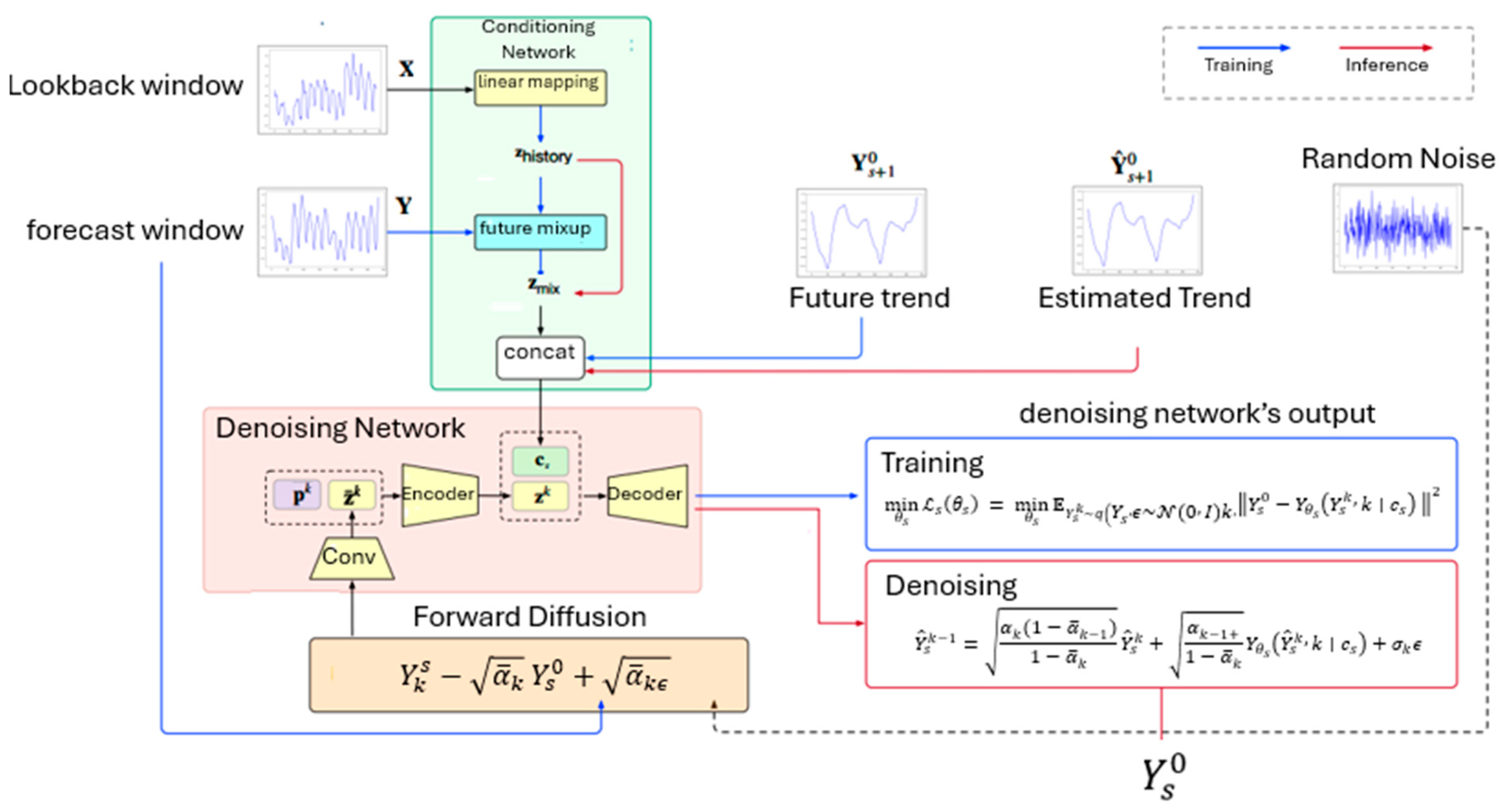
Conditioning Network: A linear projection is performed to X s in order to generate a tensor z h i s t o r y R d × H to enhance denoising performance during training, and the future-guided mixup technique strategy proposed by Shen et al. [30] is employed. This technique augments z h i s t o r y by combining it with the actual future observation Y s 0 through a mixup mechanism:
z m i x = m z h i s t o r y + ( 1 m ) Y s 0 ,
where   stands for the Hadamard product and m [ 0 , 1 ) d × H represents a combination matrix, with each element independently sampled from a uniform distribution. The future-guided mixup technique approach is conceptually related to the supervised forcing technique, in which ground-truth signals are blended with model predictions during autoregressive decoding. In addition to the use of X s during training, the broader-scale trend Y s + 1 provides contextual information that helps refine the finer trend Y s . Therefore, the concatenation of z m i x and Y s + 1 0 across the depth dimension is performed to construct the conditioning tensor c s 2 d × H . For the final stage ( s = S ) , no broader-scale trend is available; hence, c s is set equal to z m i x .
During inference, the ground-truth Y s 0 is unavailable, which makes the application of future mixup infeasible. Consequently, z m i x is replaced by z h i s t o r y . Furthermore, as the ground-truth broader-scale trend Y s + 1 is also inaccessible, the estimate Y s 0 , generated from stage s + 2 , is concatenated with z h i s t o r y to form the condition c S .
Denoising Network: During step k in stage s + 1 , the denoising process is modeled as follows:
p θ s ( Y s k 1 Y s k , c s ) = N ( Y s k 1 ; μ θ s ( Y s k , k c s , σ k 2 I ) ) , k = 1 , , K
where θ denotes the parameters of both the conditioning process and denoising networks at stage s + 1 . The mean term is defined as follows:
μ θ s ( Y s k , k c s , σ k 2 I ) = α k ( 1 α ¯ k 1 ) 1 α ¯ k 1 Y s k + α ¯ k 1 β k 1 α ¯ k 1 Y θ s ( Y s k , k c s ) .
where Y θ s ( Y s k , k c s ) is an estimate of the ground-truth Y s 0 , which is consistent with the formulation in DDPM [5]. The denoising network, illustrated in Figure 3, generates Y θ s ( Y s k , k c s ) under the guidance of the condition c s , provided by the conditioning network. Specifically, the input Y s k is first transformed into an embedding z ¯ k R d × H through an input projection block comprising several convolutional layers. The embedding z ¯ k , together with the diffusion-step embedding p k R d introduced in (8), is subsequently processed by a convolutional encoder to obtain a representation tensor z k R d × H . Next, the representation z k is concatenated with the conditioning csc_s within the variable dimension, yielding a tensor of shape ( 2 d + d ) × H . This concatenated tensor is then fed into a convolutional decoding module, which produces the output Y θ s ( Y s k , k c s ) .
Analogous to the objective in DDPM [5], the parameters θ are optimized by minimizing the denoising loss:
min θ s L s ( θ s ) = min θ s E Y s k ~ q ( Y s , ϵ ~ N ( 0 , I ) , k Y s 0 Y θ s ( Y s k , k c s ) 2
When the diffusion step index satisfies k > 1 , a Gaussian perturbation ϵ ~ N ( 0 , I ) is introduced; otherwise, ϵ = 0 . Under this condition, each denoising transition from the current estimate Y ^ s k of Y s k to the refined estimate Y ^ s k 1 is expressed as follows:
Y ^ s k 1 = α k ( 1 α ¯ k 1 ) 1 α ¯ k Y ^ s k + α k 1 + 1 α ¯ k Y θ s ( Y ^ s k , k c s ) + σ k ϵ

4.5. Synthetic Dataset Configuration

Two 10,000-step synthetic datasets were generated:
  • Laplace noise series: scale b = 0.5, μ = 0, representing heavy-tailed noise.
  • Heteroskedastic series: variance σ2t = 0.1 + 0.05 sin 2πt/500); mapping f(xt1) = 0.7xt1 + 0.2xt13 + εt.
These assess robustness to non-Gaussian and time-varying variance conditions.

4.6. Ablation Study

Ablation analysis varied as follows:
(i)
Number of stages S ∈ {2, 3, 4};
(ii)
Embedding dimension d ∈ {64, 128, 256};
(iii)
Forecast horizon H ∈ {12, 24, 48}.
Results show S = 3 and d = 128 offer the best trade-off between accuracy and efficiency; increasing S > 4 improves MSE by < 1% but extends training time by ≈ 35%.

5. Dataset

5.1. Synthetic Datasets

To assess the effectiveness of diffusion models in forecasting under non-ideal conditions, two synthetic time-series datasets were constructed to emulate challenging scenarios frequently observed in real-world applications.
Non-Gaussian Heavy-Tailed Noise (Laplace): This dataset was generated to represent time series corrupted by Laplace-distributed noise, which is characterized by sharp peaks and heavy tails. It was designed to evaluate the robustness of the model against non-Gaussian disturbances and the presence of outliers. When the data are corrupted by heavy-tailed distributions, the noise ϵ t is sampled from a Laplace distribution:
ϵ t L a p l a c e ( 0 , b ) ,
where b controls the scale of the distribution. The Laplace distribution introduces sharp peaks at the mean and heavier tails compared to Gaussian noise. This dataset is designed to examine the model’s robustness against non-Gaussian disturbances and extreme outliers.
Non-linear Heteroskedastic Series: This dataset was designed to exhibit non-linear temporal dynamics together with heteroskedastic variance patterns, i.e., variance depending on time. Its purpose was to examine the ability of the model to adapt to complex, non-stationary structures with varying degrees of uncertainty. When time-dependent variance and non-linear behavior dominate, the series is generated as follows:
X t = f ( X t 1 , , X t p ) + σ t ϵ t
where f ( ) represents a non-linear autoregressive mapping, and σ t 2 denotes time-varying variance defined as follows:
σ t 2 = α + β X t 1 2 + γ σ t 1 2 ,
with α , β , γ > 0 . This construction reflects heteroskedastic variance patterns (e.g., GARCH-type processes), allowing the model’s capacity to adapt to non-stationary time series with evolving uncertainty to be tested.
Both datasets were configured to allow control and variation in noise levels, with each consisting of 10,000 time steps. Illustrative examples of high and low noise levels for the Laplace and heteroskedastic datasets, using the first 1000 time steps, are presented in Figure 4 and Figure 5, respectively. For clarity of visualization, only a single time series ( X m , 1 : 1000 0 ) is displayed.

5.2. Real-World Datasets

We utilized real-world water-quality datasets provided by the Metropolitan Waterworks Authority in Thailand. The data were collected from several monitoring stations along the Chao Phraya River, including the Mae Klong, Khwae Noi, and Khwae Yai Rivers, and the Port Authority of Thailand. Each dataset consists of a multivariate time series with measurements recorded every 10 min. The recorded variables include temperature, conductivity, total dissolved solids (TDS), pH, and chlorophyll concentration. During preprocessing, we observed that the dataset contained missing values, likely due to sensor errors or data transmission issues. To address this issue, we aggregated the data from 10 min intervals to hourly intervals before using it for training and forecasting in our experiments. These datasets are publicly available on the Thai government open data portal [12].

6. Evaluation Setting

All experiments were conducted using Python 3.11 and executed on a system equipped with an NVIDIA RTX 2060 GPU with 8 GB of RAM.

6.1. LSTM Baseline for Comparison

To establish a baseline for performance evaluation, a standard long short-term memory (LSTM) model was employed. The LSTM was trained using identical input and output window configurations to those of the proposed method, thereby ensuring a fair basis for comparison. The model was optimized with the mean squared error (MSE) loss function and implemented with a single hidden layer containing a fixed number of hidden units, with the latter determined through validation.
In order to extend the LSTM to a generative forecasting framework, a Monte Carlo approach with dropout at inference time was applied, as formulated in the following (17):
X t , R + 1 : T 1 M m 1 M X t , R + 1 : T ( m )
This approach enabled the estimation of predictive uncertainty and ensured a fair comparison between the LSTM baseline and the proposed diffusion-based method.

6.2. Evaluation Metrics

The performance of the forecasting models was evaluated using both deterministic and probabilistic metrics. The deterministic metrics quantify the average magnitude of error between predictions and ground-truth values, whereas the probabilistic metric evaluates the overall quality of the predictive distribution. All metrics were computed in the context of multivariate time-series forecasting, where X t , m denotes the ground-truth value for the variable m at time t , and X ^ t , m represents the corresponding predicted value.
Mean squared error (MSE): The mean squared error (MSE) is defined as the average of the squared differences between the predicted values and the corresponding ground-truth values, penalizing large deviations more severely:
M S E = 1 M H t = 1 H m = 1 M ( X ^ t , m X t , m ) 2
Mean absolute error (MAE): The mean absolute error (MAE) is defined as the average of the absolute differences between the predicted and the actual values:
M A E = 1 M H t = 1 H m = 1 M X ^ t , m X t , m
Mean absolute percentage error (MAPE): The mean absolute percentage error (MAPE) is defined as the error expressed as a percentage of the observed value. Although frequently adopted for interpretability, it becomes undefined when any X t , m = 0 :
M A P E = 100 M H t = 1 H m = 1 M X ^ t , m X t , m X t , m
Symmetric mean absolute percentage error (sMAPE): The sMAPE mitigates the limitations of MAPE by normalizing the error with the sum of absolute values of predictions and observations:
s M A P E = 100 M H t = 1 H X ^ t , m X t , m ( X ^ t , m + X t , m ) / 2
Continuous ranked probability score (CRPS): The CRPS evaluates the distance between the predicted cumulative distribution function (CDF) (F) and the observed value X t , m , thereby generalizing MAE to the probabilistic forecasting setting [4]:
C R P S F , X t , m = ( F z 1 z X t , m 2 d z .
Lower values across all metrics indicate superior predictive performance.

7. Experimental Results

7.1. Influence of Noise Level and Forecast Length on Loss in the Diffusion Model

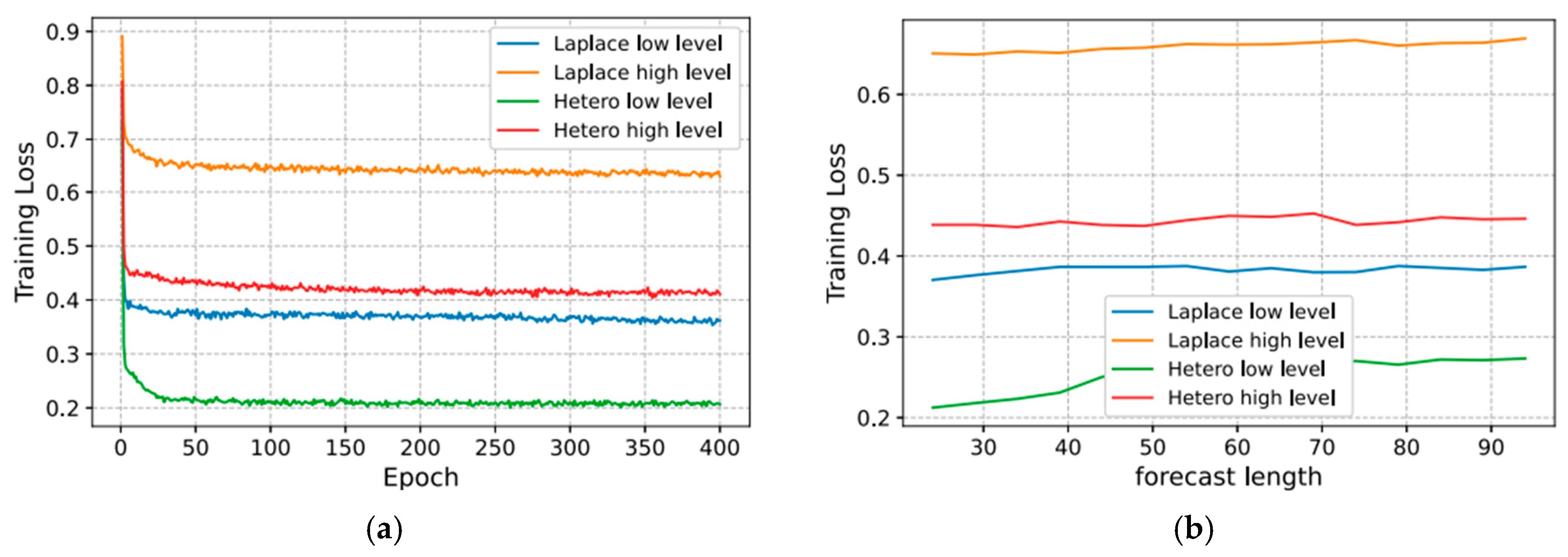
The influence of forecast length and noise level on the training dynamics of the diffusion model was first examined. In this experiment, the denoising performance was assessed by computing the mean squared error (MSE) between the predicted and actual noise at each diffusion step. This evaluation was intended to illustrate how variations in forecast configuration and noise intensity affect the model’s capacity to learn an accurate denoising function across the forward diffusion iterations. The corresponding results are presented in Figure 6. It should be noted that Laplace and Hetero represent the non-Gaussian heavy-tailed noise and non-linear heteroskedastic series datasets, respectively. As depicted in the training loss curves in Figure 6, neither the noise level nor the dataset type exerted a substantial impact on the training loss across epochs.
A consistent trend was observed across all experimental settings, with the loss stabilizing at approximately epoch 50. These results demonstrate the robustness of the diffusion model with respect to noise levels. Consequently, the number of training epochs was fixed at 50 for all subsequent evaluations. The influence of forecast length was then investigated, highlighting the inherent difficulty associated with long-horizon time-series forecasting, as discussed in [15]. The results illustrated in Figure 5 further emphasize the stability and resilience of the diffusion model when subjected to variations in forecast horizons, particularly for horizons exceeding 48 time steps. Collectively, these findings confirm that the diffusion model remains robust to changes in both noise levels and forecast length, thereby indicating that neither factor substantially affects its forecasting performance.

7.2. Forecasting Evaluation on Synthetic Datasets

We evaluated the forecasting task using all metrics described in Section 5.2. For this evaluation, each synthetic dataset was split into a training set and a testing set with a 70:30 ratio: X m , 1 : 7000 was used for training and X m , 1 : 7001 : 10000 for testing. The time series was further divided into input sequences of length 24 and forecast windows of length 24. Note that LSTM does not specifically address the concept of long-horizon forecasting, typically defined as forecasting more than 48 future time steps [15]. Therefore, we set the forecast horizon to 24 steps to ensure a fair comparison between LSTM and our proposed method. The results are shown in Table 1.
As a result, LSTM performs better on deterministic metrics, such as MAE and MSE, across most datasets, indicating a strong average point-wise accuracy. However, our diffusion model outperforms LSTM on distribution-aware metrics, such as MAPE, sMAPE, and CRPS, which better capture relative error and the quality of probabilistic forecasts. For the Laplace low-level noise dataset, LSTM achieves the lowest values across all metrics, except CRPS. This is because of the relatively low noise intensity, which allows LSTM to fit the data well without being significantly affected by outliers. In such low-noise conditions, the benefits of explicitly modeling uncertainty, as achieved by diffusion models, are less significant. In contrast, for the Laplace high-level noise dataset and both low- and high-level heteroskedastic datasets, while LSTM still performs well on MSE and MAE, it struggles with percentage-based and probabilistic metrics. On the other hand, our diffusion model shows greater robustness in handling heavy-tailed noise and time-varying variance. Lower MAPE, sMAPE, and CRPS scores demonstrate its strength in capturing uncertainty and generating reliable forecasts under complex patterns or non-Gaussian conditions. In summary, LSTM can provide robust forecasting in low-noise, deterministic settings, while the diffusion model provides superior performance in environments characterized by high uncertainty, outliers, or nonstationary behavior.

7.3. Forecasting Evaluation on Real-World Datasets

The forecasting task was further evaluated on real-world water-quality datasets using the evaluation procedure described in Section 7.2, thereby ensuring consistency with the experiments conducted on synthetic datasets. Each time series was divided into training and testing subsets with a 70:30 ratio. For these datasets, the sequences were segmented into input windows of 24 steps (equivalent to one day) and forecast horizons of 24 steps (also representing one day). The results are reported in Table 2.
The station identifiers in Table 2 are abbreviated as follows: PA refers to the Port Authority of Thailand, MK to Mae Klong, KN to Khwae Noi, and KY to Khwae Yai. As illustrated in Table 2, the forecasting performance for the temperature variable closely resembled the trends observed in the evaluation on synthetic datasets. However, a notable increase in error across all metrics was observed for the total dissolved solids (TDS) variable, affecting both the LSTM and diffusion models. This degradation in performance is represented as attributed to the absence of clear periodic patterns in the TDS series, which are typically critical for achieving accurate forecasting. In the absence of such regularities, both models encountered difficulties in capturing meaningful temporal dependencies. To gain further insight into this phenomenon, a more detailed investigation into TDS forecasting will be undertaken in collaboration with domain experts familiar with the dataset characteristics.

8. Discussion

In this study, a diffusion-based model was adopted for time-series forecasting and evaluated in the context of water-quality monitoring in the Mae Klong, Khwae Noi, and Khwae Yai Rivers. Overall, the diffusion model demonstrates strong potential as an alternative forecasting approach, as it learns a generative process capable of capturing complex data distributions in a probabilistic and flexible manner. On synthetic datasets, the model was tested under high-noise conditions, thereby enabling an assessment of its robustness in challenging scenarios. The results demonstrated that the diffusion model consistently achieved lower continuous ranked probability score (CRPS) values compared to the LSTM baseline, confirming its capacity to more effectively model uncertainty and generate forecasts that better approximate the true distribution.
By contrast, when evaluated using deterministic metrics such as mean squared error (MSE) and mean absolute error (MAE), the LSTM baseline outperformed the diffusion model. This outcome is attributable to the fact that the LSTM is optimized specifically for pointwise predictions, whereas the diffusion model is designed to generate predictive distributions over possible future outcomes. Consequently, the forecasts produced by the diffusion model may not always yield the lowest average error in direct pointwise comparisons. These findings highlight a fundamental trade-off between probabilistic accuracy and pointwise predictive accuracy. While the LSTM demonstrates superiority in minimizing direct prediction error, diffusion models provide forecasts that better encapsulate the underlying uncertainty and variability inherent in time-series data. The results suggest that the diffusion-based framework offers a more informative and resilient forecasting paradigm, particularly in domains where uncertainty quantification and robustness to non-stationarity are of critical importance.
The MDF framework demonstrates that integrating multi-scale trend decomposition with diffusion-based generative forecasting enhances robustness under noisy and uncertain environments. On synthetic datasets, MDF consistently achieved lower CRPS and sMAPE values, confirming stronger probabilistic calibration. However, deterministic baselines, such as LSTM, produced lower MAE/MSE for short-horizon forecasts, indicating that diffusion models trade point-wise precision for distributional expressiveness.

9. Conclusions

Beyond numerical improvements, the MDF framework provides actionable intelligence for sustainability-oriented water governance. Accurate short-term and probabilistic forecasts enable water authorities to achieve the following:
  • Anticipate contamination events and deploy mitigation resources early;
  • Protect public health and freshwater ecosystems;
  • Enhance resilience of river systems against climate-induced variability and inform evidence-based environmental policy and planning.
By facilitating reliable uncertainty-aware predictions, MDF contributes to sustainable river-basin management, early-warning systems, and SDG-aligned monitoring frameworks, particularly in data-scarce and noise-sensitive aquatic environments.

9.1. Sustainability and Policy Implications

The proposed forecasting framework advances environmental sustainability in several ways (Table 3):

9.2. Limitations

Several limitations remain:
(1)
Computational cost increases with the number of diffusion steps and scales.
(2)
Incomplete seasonal modeling may limit accuracy for highly periodic data.
(3)
Underperformance in short horizons suggests that diffusion’s iterative reconstruction may introduce temporal lag.
(4)
The present study evaluates single-station training; cross-station and multi-horizon generalization require further exploration.

9.3. Future Work

Future research will explore the following:
(1)
Adaptive noise scheduling conditioned on signal variance;
(2)
Hybrid MDF-transformer architectures for long-term dependencies;
(3)
Explicit disentanglement of seasonal-trend residuals;
(4)
Multi-task learning to unify imputation and forecasting.

Author Contributions

Conceptualization, W.R. and R.F.; Methodology, R.F.; Writing—original draft, R.F.; Writing—review & editing, R.F.; Supervision, R.F.; Project administration, W.R.; Funding acquisition, R.F. All authors have read and agreed to the published version of the manuscript.

Funding

This research received no external funding.

Institutional Review Board Statement

Not applicable.

Informed Consent Statement

Not applicable.

Data Availability Statement

The original contributions presented in this study are included in the article. Further inquiries can be directed to the corresponding author.

Conflicts of Interest

The authors declare no conflict of interest.

Appendix A

  Algorithm A1. Multi-scale denoising process
  Input:
                Time series segments:  ( X 0 , Y 0 ) q ( X , Y )
                Number of diffusion steps:  K
                Number of scales:  S
  Procedure:
                Initialization:
                Extract multi-scale trend components:
                                   { X s } s = 1 S 1 = T r e n d E x t r a c t i o n ( X 0 ) , { Y s } s 1 S 1 = T r e n d E x t r a c t i o n ( Y 0 )  
                Training Loop:
                Repeat until convergence:
                                                               F o r s = S 1 , S 2 , , 0 ;
                                  2.1. Sample diffusion step index:
                                                               k U n i f o r m ( { 1,2 , , K } )
                                  2.2. Sample Gaussian noise:
                                                              ϵN(0,I)
                                  2.3. Generate diffused sample:
                                                               Y k s α ¯ k Y s 0 + α ¯ k ϵ
                                  2.4. Obtain diffusion embedding p k (Equation (6)).
                                  2.5. Randomly generate matrix m (Equation (9)).
                                  2.6. Compute historical mapping:
                                                               z h i s t o r y L i n e a r X s
                                  2.7. Compute mixed representation:
                                                               z m i x f ( m , z h i s t o r y )
                                  2.8. Form condition vector:
                                            If s < S 1 :
                                                         c s z m i x , Y + 10 0 s
                                            Else:
                                                         c s z m i x
                                  2.9. Compute loss at step kkk:
                                                               L k s ( θ s ) (Equation (14)).
                                  2.10. Update parameters:
                                                               θ s θ s η θ s L k s ( θ s )
                Convergence:
                Continue until training stabilizes.
  Algorithm A2. Multi-scale inference process
  Input: Lookback sequence X 0
  Output: Final reconstructed sequence Y 0 ^

  Extract trend components:
                                                 { X S } s = 1 S 1 = T r e n d E x t r a c t i o n ( X 0 ) .
  While  s = S 1 , , 0  do
                              2.1. Compute historical embedding:
                                                   z h i s t o r y = L i n e a r M a p ( X s ) .
  2.2. If  s < S 1  then
                                                 c s = C o n c a t ( z h i s t o r y , Y s + 1 0 ) .
                      Else
                                                 c s = z h i s t o r y .
                      End If
  2.3. Initialize the diffusion variable:
                                                 Y s K ^ N ( 0 , I ) ) .
  2.4. While  k = K , , 1  do
                                                                  ϵ N ( 0 , I )   i f   k > 1 , e l s e   ϵ = 0 .
                                                Compute the step embedding p k using (8).
                                                Update denoised output by (13):
                                                                  Y ^ s K 1 = f ( Y ^ s K , p k , c s , ϵ ) .
                                                End While
  End While
  Return  Y 0 ^ .

References

  1. Bahdanau, D.; Cho, K.; Bengio, Y. Neural machine translation by jointly learning to align and translate. In Proceedings of the International Conference on Learning Representations (ICLR), San Diego, CA, USA, 7–9 May 2015. [Google Scholar]
  2. Lin, L.; Li, Z.; Li, R.; Li, X.; Gao, J. Diffusion models for time-series applications: A survey. Front. Inf. Technol. Electron. Eng. 2024, 25, 19–41. [Google Scholar] [CrossRef]
  3. Yang, L.; Zhang, Z.; Song, Y.; Hong, S.; Xu, R.; Zhao, Y.; Zhang, W.; Bin Cui, B.; Yang, M.H. Diffusion Models: A Comprehensive Survey of Methods and Applications. ACM Comput. Surv. 2023, 53, 1–39. [Google Scholar] [CrossRef]
  4. Murphy, A.H.; Winkler, R.L. A general framework for forecast verification. Mon. Weather. Rev. 1987, 115, 1330–1338. [Google Scholar] [CrossRef]
  5. Ho, J.; Jain, A.; Abbeel, P. Denoising diffusion probabilistic models. In Proceedings of the Advances in Neural Information Processing Systems (NeurIPS), Virtual, 6–12 December 2020; Volume 33, pp. 6840–6851. [Google Scholar]
  6. Bergemann, D.; Morris, S. Information design: A unified perspective. J. Econ. Lite. 2019, 57, 44–95. [Google Scholar] [CrossRef]
  7. Nichol, A.Q.; Dhariwal, P. Improved denoising diffusion probabilistic models. In Proceedings of the 38th International Conference on Machine Learning (ICML), Virtual, 18–24 July 2021; Volume 139, pp. 8162–8171. [Google Scholar]
  8. Sohl-Dickstein, J.; Weiss, E.; Maheswaranathan, N.; Ganguli, S. Deep unsupervised learning using nonequilibrium thermodynamics. In Proceedings of the 32nd International Conference on Machine Learning (ICML), Lille, France, 6–11 July 2015; Volume 37, pp. 2256–2265. [Google Scholar]
  9. Chen, M.; Mei, S.; Fan, J.; Wang, M. Opportunities and challenges of diffusion models for generative AI. Nat. Sci. Rev. 2024, 11, nwae348. [Google Scholar] [CrossRef]
  10. Liu, M.; Zeng, A.; Chen, M.; Xu, Z.; Lai, Q.; Ma, L.; Xu, Q. SCINet: Time series modeling and forecasting with sample convolution and interaction. In Proceedings of the Advances in Neural Information Processing Systems (NeurIPS), New Orleans, LA, USA, 28 November–9 December 2022; Volume 35, pp. 5816–5828. [Google Scholar]
  11. Truong, V.T.; Dang, L.B.; Le, L.B. Attacks and defenses for generative diffusion models: A comprehensive survey. ACM Comput. Surv. 2025, 57, 1–44. [Google Scholar] [CrossRef]
  12. Metropolitan Waterworks Authority. Metropolitan Waterworks Authority Headquarters. Government Data Catalog. Available online: https://gdcatalog.go.th/organization/4388d502-250d-48b3-bdcc-43c0d6f0287b (accessed on 19 March 2025).
  13. Li, J.; Chen, W.; Liu, Y.; Yang, J.; Zhou, Z.; Zeng, D. Diffinformer: Diffusion Informer model for long sequence time-series forecasting. Exp. Sys. App. 2026. Available online: https://www.sciencedirect.com/science/article/abs/pii/S0957417425035596?via%3Dihub (accessed on 19 March 2025).
  14. Vaswani, A.; Shazeer, N.; Parmar, N.; Uszkoreit, J.; Jones, L.; Gomez, A.N.; Kaiser, Ł.; Polosukhin, I. Attention is all you need. In Proceedings of the Advances in Neural Information Processing Systems (NeurIPS), Long Beach, CA, USA, 4–9 December 2017; Volume 30, pp. 5998–6008. [Google Scholar]
  15. Zhou, H.; Zhang, S.; Peng, J.; Zhang, S.; Li, J.; Xiong, H.; Zhang, W. Informer: Beyond efficient transformer for long sequence time-series forecasting. In Proceedings of the AAAI Conference on Artificial Intelligence, Virtual, 2–9 February 2021; pp. 11106–11115. [Google Scholar]
  16. Wu, H.; Xu, J.; Wang, J.; Long, M. Autoformer: Decomposition transformers with auto-correlation for long-term series forecasting. In Proceedings of the Advances in Neural Information Processing Systems (NeurIPS), Online, 6–14 December 2021; Volume 34, pp. 22419–22430. [Google Scholar]
  17. Zhou, T.; Ma, Z.; Wen, Q.; Wang, X.; Sun, L.; Jin, R. FED former: Frequency enhanced decomposed transformer for long-term series forecasting. In Proceedings of the International Conference on Machine Learning (ICML), Baltimore, MD, USA, 17–23 July 2022; pp. 27268–27286. [Google Scholar]
  18. Liu, S.; Yu, H.; Liao, C.; Li, J.; Lin, W.; Liu, A.X.; Dustdar, S. Pyraformer: Low-complexity pyramidal attention for long-range time series modeling and forecasting. In Proceedings of the International Conference on Learning Representations (ICLR), Vienna, Austria, 3–7 May 2021. [Google Scholar]
  19. Shabani, M.A.; Abdi, A.H.; Meng, L.; Sylvain, T. Scaleformer: Iterative multi-scale refining transformers for time series forecasting. In Proceedings of the International Conference on Learning Representations (ICLR), Kigali, Rwanda, 1–5 May 2023. [Google Scholar]
  20. Su, J.; Xie, D.; Duan, Y.; Zhou, Y.; Hu, X.; Duan, S. MDCNet: Long-term time series forecasting with mode decomposition and 2D convolution. Knowledge-Based Sys. 2024, 299, 111986. [Google Scholar] [CrossRef]
  21. Dosovitskiy, A.; Beyer, L.; Kolesnikov, A.; Weissenborn, D.; Zhai, X.; Unterthiner, T.; Dehghani, M.; Minderer, M.; Heigold, G.; Gelly, S.; et al. An image is worth 16 × 16 words: Transformers for image recognition at scale. In Proceedings of the International Conference on Learning Representations (ICLR), Addis Ababa, Ethiopia, 26–30 April 2020. [Google Scholar]
  22. Zhou, T.; Ma, Z.; Wang, X.; Wen, Q.; Sun, L.; Yao, T.; Yin, W.; Jin, R. FiLM: Frequency improved Legendre memory model for long-term time series forecasting. In Proceedings of the Advances in Neural Information Processing Systems (NeurIPS), New Orleans, LA, USA, 28 November–9 December 2022; Volume 35, pp. 12677–12689. [Google Scholar]
  23. Oreshkin, B.N.; Carpov, D.; Chapados, N.; Bengio, Y. N-BEATS: Neural basis expansion analysis for interpretable time series forecasting. In Proceedings of the International Conference on Learning Representations (ICLR), New Orleans, LA, USA, 6–9 May 2019. [Google Scholar]
  24. Fan, W.; Zheng, S.; Yi, X.; Cao, W.; Fu, Y.; Bian, J.; Liu, T.-Y. DEPTS: Deep expansion learning for periodic time series forecasting. In Proceedings of the International Conference on Learning Representations (ICLR), Virtual, 25–29 April 2022. [Google Scholar]
  25. Challu, C.; Olivares, K.G.; Oreshkin, B.N.; Garza, F.; Mergenthaler-Canseco, M.; Dubrawski, A. N-HITS: Neural hierarchical interpolation for time series forecasting. In Proceedings of the AAAI Conference on Artificial Intelligence, Washinton, DC, USA, 7–14 February 2023. [Google Scholar]
  26. Zeng, A.; Chen, M.; Zhang, L.; Xu, Q. Are transformers effective for time series forecasting? In Proceedings of the AAAI Conference on Artificial Intelligence, Washinton, DC, USA, 7–14 February 2023; pp. 11121–11129. [Google Scholar]
  27. Rasul, K.; Seward, C.; Schuster, I.; Vollgraf, R. Autoregressive denoising diffusion models for multivariate probabilistic time series forecasting. In Proceedings of the International Conference on Machine Learning (ICML), Virtual, 18–24 July 2021; pp. 8827–8837. [Google Scholar]
  28. Tashiro, Y.; Song, J.; Song, Y.; Ermon, S. CSDI: Conditional score-based diffusion models for probabilistic time series imputation. In Proceedings of the Advances in Neural Information Processing Systems (NeurIPS), Online, 6–14 December 2021; Volume 34, pp. 24804–24816. [Google Scholar]
  29. Lugmayr, A.; Danelljan, M.; Romero, A.; Yu, F.; Timofte, R.; Van Gool, L. RePaint: Inpainting using denoising diffusion probabilistic models. In Proceedings of the IEEE/CVF Conference on Computer Vision and Pattern Recognition (CVPR), New Orleans, LA, USA, 18–24 June 2022; pp. 11461–11471. [Google Scholar]
  30. Shen, L.; Kwok, J. Non-autoregressive conditional diffusion models for time series prediction. In Proceedings of the International Conference on Machine Learning (ICML), Honolulu, HI, USA, 23–29 July 2023. [Google Scholar]
  31. Bui, K.H.N.; Cho, J.; Yi, H. Spatial-temporal graph neural network for traffic forecasting: An overview and open research issues. App. Intel. 2022, 52, 2763–2774. [Google Scholar] [CrossRef]
  32. Ronneberger, O.; Fischer, P.; Brox, T. U-Net: Convolutional networks for biomedical image segmentation. In Proceedings of the Medical Image Computing and Computer-Assisted Intervention (MICCAI), Munich, Germany, 5–9 October 2015; pp. 234–241. [Google Scholar]
  33. Niu, H.; Meng, C.; Cao, D.; Habault, G.; Legaspi, R.; Wada, S.; Ono, C.; Liu, Y. Mu2ReST: Multi-resolution recursive spatio-temporal transformer for long-term prediction. In Proceedings of the Pacific-Asia Conference on Knowledge Discovery and Data Mining (PAKDD), Chengdu, China, 16–19 May 2022; pp. 79–91. [Google Scholar]
  34. Ma, X.; Li, Y.; Zhang, H. An U-Mixer architecture with stationarity correction for long-term time series forecasting. In Proceedings of the AAAI Conference on Artificial Intelligence (Vol. 38, No. 1), Vancouver, BC, Canada, 20–27 February 2024; pp. 1234–1243. [Google Scholar]
  35. Jeha, P.; Bohlke-Schneider, M.; Mercado, P.; Kapoor, S.; Nirwan, R.S.; Flunkert, V.; Gasthaus, J.; Januschowski, T. PSA-GAN: Progressive self-attention GANs for synthetic time series. In Proceedings of the International Conference on Learning Representations (ICLR), Virtual, 25–29 April 2022. [Google Scholar]
  36. Ho, J.; Saharia, C.; Chan, W.; Fleet, D.J.; Norouzi, M.; Salimans, T. Cascaded diffusion models for high fidelity image generation. J. Mach. Learn. Res. 2022, 23, 1–33. [Google Scholar]
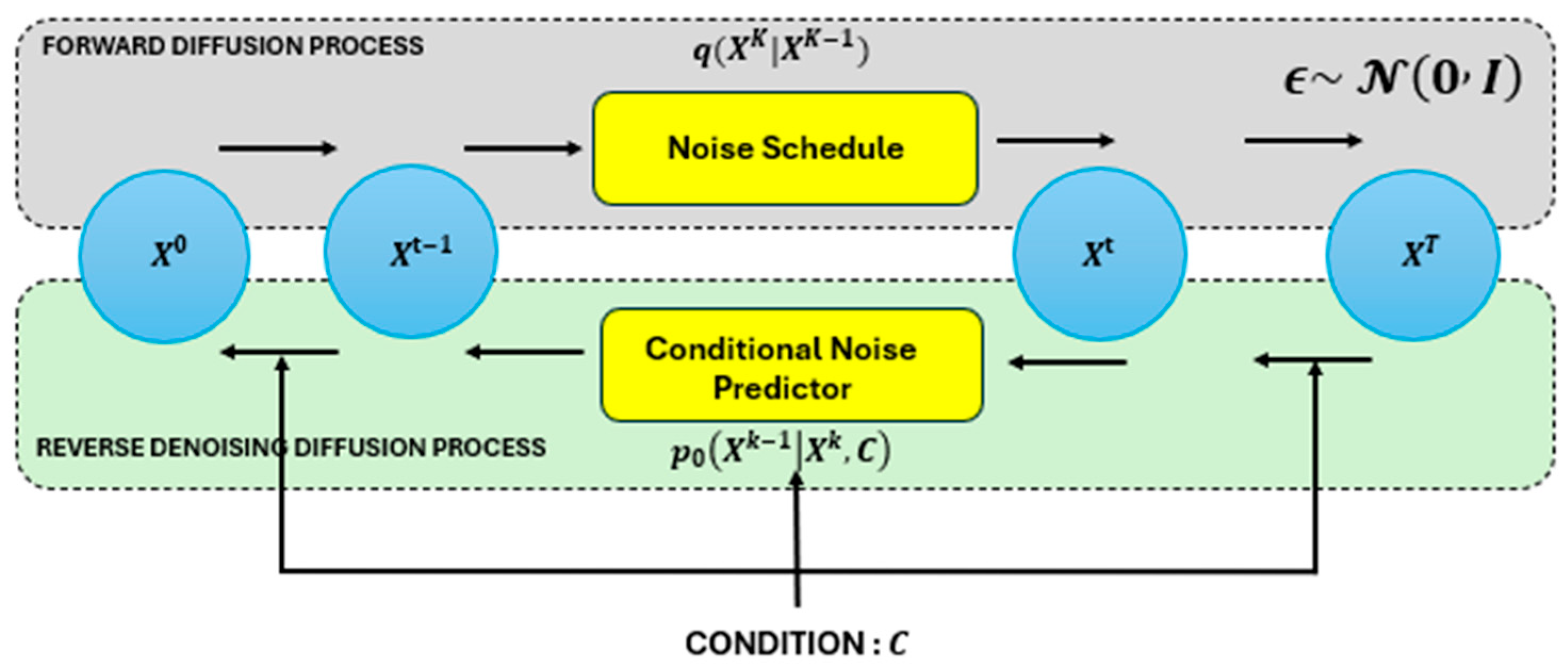
Figure 1. The forward and reverse diffusion processes in the diffusion model.
Sustainability 17 10295 g001
Figure 2. Block diagram of the proposed multi-scale diffusion forecaster (MDF) framework.
Sustainability 17 10295 g002
Figure 3. The condition and denoising network process.
Sustainability 17 10295 g003
Figure 4. Non-Gaussian heavy-tailed noise (Laplace) at varying noise levels.
Sustainability 17 10295 g004
Figure 5. Non-linear heteroskedastic series at varying noise levels.
Sustainability 17 10295 g005
Figure 6. The results of (a) training loss over epochs across different datasets and (b) influence forecast length on training loss across different datasets.
Sustainability 17 10295 g006
Table 1. Forecasting performance comparison between MDF and LSTM on synthetic datasets.
Metrics
Dataset NameMethodsMSEMAEMAPEsMAPECRPS
Laplace Low-levelLSTM0.08930.21185410.149248.222000.3629
MDF0.09880.25460438.063164.479350.2546
Laplace High-levelLSTM0.524400.51110562.457274.28020.84835
MDF0.783750.70015486.609119.42550.70015
Hetero Low-levelLSTM0.022800.111153432.83124.904250.17670
MDF0.019950.11020125.268030.825600.11020
Hetero High-levelLSTM0.130150.26030306.178471.07520.40470
MDF0.148200.31255166.532247.60070.32395
The best-performing values for each metric and dataset are both bolded and underlined.
Table 2. Forecasting performance comparison between MDF and LSTM on the water-quality dataset from the Port Authority of Thailand (PA), Mae Klong (MK), Khwae Noi (KN), and Khwae Yai Rivers (KY).
Metrics
Dataset NameMethodsMSEMAEMAPEsMAPECRPS
PA (TEMP)LSTM1.554650.951153.099103.170500.91545
MDF2.040002.800753.003052.759950.90695
PA (TSD)LSTM34,992.15158.043951.1224074.46170151.5729
MDF37,029.26207.329558.6100581.95105191.7974
MK (TEMP)LSTM1.394850.912052.95123.02090.90950
MDF2.121602.424204.36732.64521.41695
MK (TSD)LSTM10,449.0386.2597042.5263557.2611080.68965
MDF24,054.05217.968120.1790033.9005547.92640
KN (TEMP)LSTM1.665150.908652.859402.941000.95965
MDF3.767207.934754.544954.990351.66515
KN (TSD)LSTM14,337.38110.167752.747676.52380105.5513
MDF34,243.71388.095646.840128.4877576.93605
KY (TEMP)LSTM2.025551.13223.609953.715351.00300
MDF1.759501.41612.980952.878100.96305
KY (TSD)LSTM3305.9152.6736530.7887037.6652046.22640
MDF16,599.9680.9327530.3424518.7841543.63305
The best-performing values for each metric and dataset are both bolded and underlined.
Table 3. Sustainability implications.
Sustainability DomainContribution of Proposed MDF Model
Public health and safe waterEarly detection of pollution risk for communities
Ecosystem preservationProtects biodiversity through proactive water-quality surveillance
Climate adaptationSupports resilience planning under hydrological uncertainty
Sustainable development policyAligns with SDGs 6, 13, and 14 for clean water and ecosystem protection
Resource optimizationSupports cost-efficient monitoring and intervention scheduling
Disclaimer/Publisher’s Note: The statements, opinions and data contained in all publications are solely those of the individual author(s) and contributor(s) and not of MDPI and/or the editor(s). MDPI and/or the editor(s) disclaim responsibility for any injury to people or property resulting from any ideas, methods, instructions or products referred to in the content.