Source Apportionment of Urban GHGs in Hong Kong from Regional Transportation Based on Diagnostic Ratio Method

Abstract

Quantifying the regional source of long-lived ozone precursors (especially GHGs) transported to Hong Kong is hampered by sparse observational data and computational limitations. This study introduces an observation-driven analytical framework that integrates a tracer ratio (ethylbenzene/m,p-xylene), wind–source–distance correlations to constrain transport corridors, and inventory mapping to determine the province- and sector-specific contributions, operationalized by identifying transport periods from observations, classifying sources with diagnostic ratios into five emission categories, deriving seasonal weighting factors via frequency normalization, mapping high-resolution inventory classes to these categories to restructure sectoral inventories, and combining normalized provincial spatial weights with the restructured inventories to quantify cross-boundary CO₂ and CH₄ emissions by sector and region. High-resolution measurements were conducted at the Cape D’Aguilar Supersite (CDSS), which showed dominant wintertime regional transport with mean concentrations of 435.29 ± 7.64 ppm (CO₂) and 2083.45 ± 56.50 ppb (CH₄). Thirteen transport periods were quantitatively analyzed, and province–sector contributions were estimated. The dominant provincial contributors were Guangdong (20.66%), followed by Jiangxi (18.36%) and Zhejiang (11.15%). Motor vehicles (70%), fuel combustion (15%), and solvent use (10%) were the primary contributing sectors. The framework enables province- and sector-specific attribution under stated assumptions and provides a tool for measuring cross-boundary mitigation and developing air quality and climate strategies in monsoon-affected coastal cities.

1. Introduction

Carbon dioxide (CO₂) and methane (CH₄) are two major long-lived greenhouse gases (GHGs) within the Earth system, contributing about 65% and 17% of the total radiative forcing, respectively [1]. According to the WMO Bulletin (2023) [2], global atmospheric concentrations reached 417.9 ± 0.2 ppm for CO₂ and 1923 ± 2 ppb for CH₄ in 2022, representing increases of ~50% and ~164% relative to pre-industrial levels. Anthropogenic CO₂ is primarily emitted from fossil fuel combustion (~85% of total emissions) and removed via photosynthetic assimilation and oceanic uptake [3]. CH₄ emissions arise from both natural sources (e.g., wetlands and marine ecosystems) and anthropogenic activities (e.g., energy production and agriculture), with removal largely through oxidation by tropospheric hydroxyl radicals and soil uptake [4].

In Hong Kong, ambient air quality trends have shown a marked divergence over the past decade. The annual average PM_2.5 concentration declined by 52.4%, from 32.46 μg/m³ in 2013 to 15.44 μg/m³ in 2024, while the ozone concentration increased by 49.2% over the same period, rising from 36.57 μg/m³ to 54.56 μg/m³. The existing control strategies have primarily focused on end-of-pipe mitigation and have provided diminishing returns [5,6,7]. Recent studies suggest that achieving both air quality improvement and climate change mitigation is needed for effective regional atmospheric management [8]. GHGs, due to their long atmospheric lifetimes and strong propensity to mix together, have emerged as essential indicators for integrated environmental governance in coastal and urban regions [9,10,11,12].

Hong Kong is located along the East Asian–Western Pacific monsoon channel, which results in a strong seasonality in pollutant transport. During winter, continental anticyclones facilitate northerly airflow, transporting pollutants from the Pearl River Delta (PRD) and mainland regions of China to Hong Kong, accounting for 35–45% of its pollutant levels [13]. In summer, southwesterly monsoons deliver 15–20% of pollution from Southeast Asia, primarily originating from biomass burning [14,15]. Diurnal land–sea-breeze circulation further complicates pollutant dispersion within Hong Kong’s coastal boundary layer [16,17]. Precise and meticulous source attribution will be the focal point of Hong Kong’s next phase in environmental governance.

Existing source-apportionment approaches include receptor modeling, trajectory analysis, and chemical transport models (CTMs). Receptor models use multivariate factorization to deduce source categories and quantify their contributions based on observed chemical profiles [18,19,20,21]. While they can provide quantitative estimates, their accuracy depends heavily on the fidelity of the source profiles, which often require resource-intensive laboratory work and expert judgment. Trajectory analysis, which uses Lagrangian particle-dispersion models such as HYSPLIT, identifies potential source regions based on pollutant advection pathways and readily available meteorological data [22]. However, spatial accuracy can be sensitive to the choice of concentration thresholds. CTMs simulate pollutant dynamics by integrating high-resolution meteorological fields and emission inventories, but they require substantial computational resources [23,24]. Recent Hong Kong studies have advanced source quantification using enhanced CMB/PMF (dynamic gas–particle partitioning and profile correction) [25], online PTR-MS coupled with PMF and trajectory clustering [26], and CTM characteristic-ratio/tracer diagnostics [27]; collectively, these approaches refine traffic apportionment, isolate biomass-burning influences, and quantify upwind transport.

However, current research primarily focuses on PM_2.5. Studies that apportion the transboundary contributions of specific provinces and sectors to long-lived GHGs (CO₂ and CH₄) transported to Hong Kong remain limited. To address this gap, we develop an observation-driven empirical-weighting framework that combines diagnostic VOC ratios for screening, trajectory-derived provincial spatial weights, and reconstructed province–sector inventories to semi-quantitatively attribute winter cross-boundary CO₂ and CH₄ transport. Unlike receptor factorization or full-physics CTM inversions, the framework avoids case-specific dynamical simulations and iterative inversions; reduces model dependence; and enables rapid, transparent, and reproducible assessments with light computational demands, supporting timely policy prioritization.

2. Instruments and Analytical Tools

2.1. Observation Site

Hong Kong is located along the southeastern coast of China, approximately 140 km east of the Pearl River Estuary (22.25–22.62° N, 113.87–114.50° E, as illustrated in Figure 1). It borders Shenzhen (Guangdong Province) to the north, Macao to the west, and the South China Sea to the east. The atmospheric observations in this study were conducted at the Cape D’Aguilar Supersite (CDSS; 22.22° N, 114.24° E), which monitors over 100 atmospheric parameters, including trace gases, oxidation radicals, volatile organic compounds (VOCs), ozone-depleting substances (ODSs), and records remote-sensing profiles of ozone, aerosols, and winds [26]. The absence of significant industrial activity and the low population density within a 5 km radius make CDSS well-suited for evaluating the influence of regional pollutant transport. Measurements were conducted during the winter season (December 2022 to February 2023) to capture the influence of continental monsoonal outflow on GHG levels in Hong Kong.

2.2. Apparatus and Data Source

2.2.1. Online Measurements

Atmospheric CO₂ and CH₄ were continuously measured using an online GHG analyzer (G2301, Picarro Inc., Santa Clara, CA, USA) that is based on cavity ring-down spectroscopy (CRDS). The operating principles of the instrument are described in detail in Crosson (2008) and Chen et al. (2009) [28,29]. Raw measurements were recorded at sub-5-s intervals, and data were averaged to a temporal resolution of one hour for the analysis. The measurement precision for CO₂ was better than 0.025 ppm (5 min, 1σ), with a maximum monthly peak deviation of 0.5 ppm. For CH₄, the precision exceeded 0.22 ppb (5 min, 1σ), with a maximum drift of 3 ppb per month. Ambient air was sampled through polytetrafluoroethylene (PTFE) tubing, with the inlet positioned 6 m above ground level. Prior to analysis, the air passed through a heated glass manifold (Model 1004, Sabio Environmental, Round Rock, TX, USA) maintained at 50 °C. A bypass sampling line was used to maintain a stable flow rate of 0.4 L min⁻¹ to the analyzer, minimizing pressure fluctuations and condensation within the sampling system. The CRDS analyzer was periodically calibrated using CO₂ and CH₄ standard gases certified by the U.S. Environmental Protection Agency. The calibration curves for both gases exhibited excellent linearity (R² > 0.999).

Calibration and QA/QC

The calibration and QA/QC followed a verification protocol. Each month, zero checks for CO₂ and CH₄ were performed using 99.999% UHP N₂, and span checks were conducted with certified standards. The predefined acceptance limits were as follows: span ≤ ±10%; zero limits for CH₄ ≤ ±0.15 ppm and CO₂ ≤ ±15 ppm. All checks remained within these limits. No significant drifts from the standard gases, which were verified by NIST within the validity period, were observed over the measurement period. In parallel, field blanks (canisters connected to the sampling manifold) were collected and analyzed monthly; the CO₂ and CH₄ levels in all blanks were below their detection limits (CO₂ < 0.01 ppm; CH₄ < 20 ppb), confirming negligible system contamination.

2.2.2. Laboratory Analysis

Ambient air samples for the GHG and VOC analyses were collected concurrently with online GHG measurements using a VOC sampler (Model 2200, ATEC, Malibu, CA, USA). Air was drawn into pre-evacuated stainless-steel canisters under controlled flow conditions. The sampling procedure strictly followed the U.S. Environmental Protection Agency (USEPA) TO-14A and TO-15 protocols. A total of 15 wintertime samples were collected and analyzed by the research group of Professor Donald R. Blake at the University of California, Irvine (UCI), using a gas-chromatography system as described by Blake et al. (1994) [30]. Analytical traceability was maintained through a two-tier calibration hierarchy involving primary standards established in 1977 and secondary standards certified by the National Bureau of Standards (NBS) in August 1982, with an uncertainty of ±1%. Quality control was ensured by alternating analyses of calibration standards with ambient air samples. The analytical repeatability was better than 2 ppbv for the target VOCs.

2.2.3. Meteorological Parameters

A three-dimensional sonic anemometer (IRGASON, Campbell Scientific, Logan, UT, USA), integrated with an open-path gas analyzer, was deployed at the CDSS to obtain high-resolution measurements of wind speed, wind direction, and air temperature. The operating principles of the system are described in Horst et al. (2016) and Zhou et al. (2018) [31,32]. The instrument performance specifications are as follows: the horizontal wind-speed components (u_x and u_γ) have an accuracy better than 1 mm s⁻¹, with a maximum drift of ±8 cm s⁻¹; the vertical wind-speed component (u_z) maintains an accuracy better than 0.5 mm s⁻¹ and a maximum drift of ±4 cm s⁻¹; wind direction is measured over the full 0–360° range with an accuracy of 0.6°; and air temperature is measured within −50 °C to 60 °C, with an accuracy of 0.025 °C.

2.2.4. Other Data Sets and Analytical Tools

Additional CO₂ and CH₄ data from six global background stations—Mauna Loa (MLO), Mauna Kea (MKO), Lulin (LLN), Minamitorishima (MNM), Ryori (RYO), and Gosan (GSN)—were obtained from the WMO Global Atmosphere Watch (GAW) World Data Centre for Greenhouse Gases (WDCGG) (WDCGG, 2025) operated by the Japan Meteorological Agency [33].

Provincial monthly CO₂ emissions, disaggregated across 52 sectors for December 2022–February 2023, were sourced from the Multi-resolution Emission Inventory for China (MEIC) [34,35,36,37].

Meteorological inputs were taken from the NCEP global reanalysis data set using a 1° × 1° resolution (NCEP/NWS/NOAA/U.S. Department of Commerce, 2015 [38]). Atmospheric transport was simulated using NOAA’s Hybrid Single-Particle Lagrangian Integrated Trajectory (HYSPLIT, version 5.2.1) model [22,39].

3. Results and Discussion

3.1. Characteristics of CO₂ and CH₄ Levels in Winter

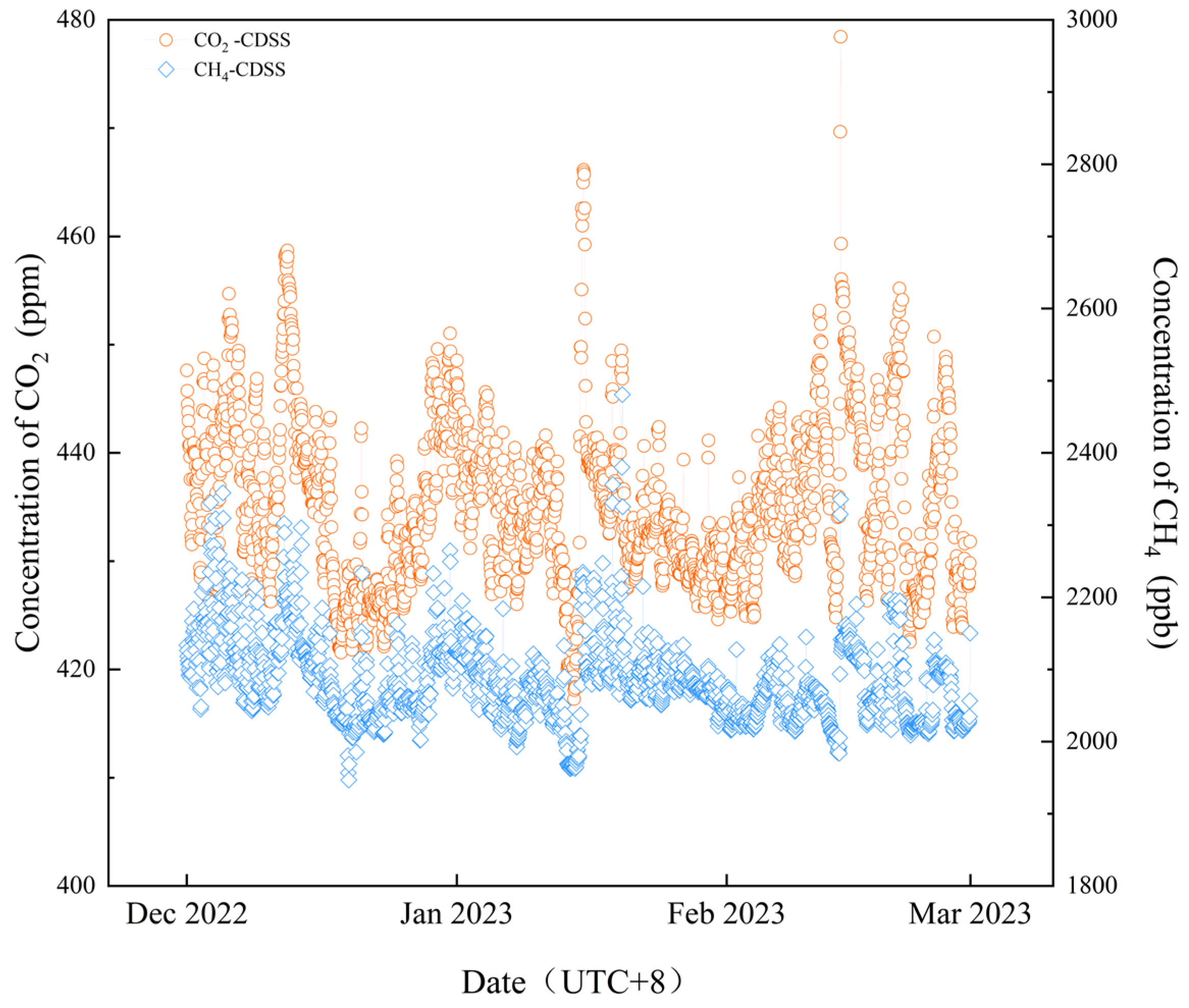
The online continuous monitoring results for CO₂ and CH₄ levels from December 2022 to February 2023 are presented in Figure 2. The CO₂ time series showed a maximum hourly concentration of 478.4 ppm, a minimum of 417.3 ppm, and a mean of 435.29 ± 7.64 ppm (1σ). The CH₄ concentrations ranged from a minimum of 1946.9 ppb to a maximum of 2480.8 ppb, with a mean of 2083.45 ± 56.50 ppb. Among the winter months, February recorded the highest mean CO₂ level (436.11 ± 7.96 ppm), followed by December (435.81 ± 8.28 ppm) and January (434.04 ± 6.46 ppm). In contrast, the highest monthly mean CH₄ concentration was observed in December (2102.06 ± 61.81 ppb), followed by January (2082.12 ± 52.77 ppb) and February (2063.83 ± 46.57 ppb). Comparisons with global GHG monitoring stations are summarized in

Table 1. Comparison of CO₂ and CH₄ levels at CDSS and other global monitoring stations.

Site	Latitude	Longitude	CO2 Maximum	CO2 Minimum	CO2 Mean	CH4 Maximum	CH4 Minimum	CH4 Mean	Data Sources
	(North: +; South: −)	(East: +; West: −)	(ppm)	(ppm)	(ppm)	(ppb)	(ppb)	(ppb)
MLO	19.54	−155.58	424.42	418.81	420.11 ± 1.31	1952.34	1929.34	1939.38 ± 8.98	WDCGG
MKO	19.83	−155.48	425.53	416.01	419.76 ± 0.98	1989.31	1901.68	1943.57 ± 12.16	WDCGG
CDSS	22.22	114.25	478.44	417.27	435.29 ± 7.64	2480.84	1946.92	2083.45 ± 56.50	This study
LLN	23.47	120.87	424.99	419.30	422.05 ± 1.73	1983.87	1926.67	1967.31 ± 15.59	WDCGG
MNM	24.29	153.98	429.84	417.48	422.08 ± 1.85	2021.00	1930.00	1979.25 ± 16.32	WDCGG
GSN	33.29	126.16	455.65	420.63	430.11 ± 5.21	2215.32	1986.08	2040.22 ± 32.36	WDCGG
RYO	39.03	141.82	454.12	420.74	427.53 ± 3.37	2072.00	1986.00	2018.59 ± 13.32	WDCGG

Notes: (1) +/− denotes north latitude (east longitude)/south latitude (west longitude). (2) The uncertainty in the table is 1 standard deviation. (3) MLO (Mauna Loa Observatory, Hawaii, USA), MKO (Mauna Kea Observatory, Hawaii, USA), LLN (Lulin Observatory, Taiwan, China), MNM (Minamitorishima, Japan), GSN (Gosan Station, Jeju, Republic of Korea), RYO (Ryori Observatory, Iwate, Japan). (4) Data from all stations except LLN and MLO (which are flask samples) are derived from automated online monitoring systems. (5) All data are sourced from the World Data Centre for Greenhouse Gases (WDCGG; https://gaw.kishou.go.jp/, accessed on 15 May 2025). (6) All station statistics are derived from the same period (December 2022–February 2023).

, including Mauna Loa (MLO, 19.54° N, 155.58° W) and Mauna Kea (MKO, 19.83° N, 155.48° W) in the United States, Lulin (LLN, 23.47° N, 120.87° E) in Taiwan, Minamitorishima (MNM, 24.29° N, 153.98° E) and Ryori (RYO, 39.03° N, 141.82° E) in Japan, and Gosan (GSN, 33.29° N, 126.16° E) in South Korea. The comparison shows that the mean CO₂ concentration at CDSS was higher than those at MLO, MKO, RYO, MNM, GSN, and LLN by 15.18, 15.53, 7.76, 13.21, 5.18, and 13.24 ppm, respectively. Similarly, the mean CH₄ concentration at CDSS exceeded those at the same stations by 144.07, 139.88, 64.86, 104.20, 43.23, and 116.14 ppb, respectively. Coastal and island stations such as MLO, MKO, GSN, and MNM are influenced by marine environments similar to Hong Kong but are far from major urban centers. MLO is situated on high-altitude volcanic terrain, while GSN and MNM are in sparsely populated areas with limited industrial and transportation emissions. In contrast, Hong Kong is not only affected by emissions from transportation, power generation, and landfill operations, but is also surrounded by mountains that facilitate the accumulation of pollutants.

Stations located in regions with a subtropical monsoon climate similar to Hong Kong—such as GSN, LLN, and RYO—typically exhibit lower GHG concentrations due to limited regional industrial activity and the dominance of clean marine airflows. In contrast, the elevated concentrations observed in Hong Kong are primarily attributed to a combination of substantial local emissions and transboundary pollutant transport from mainland China, particularly from maritime shipping and cross-border freight activities, which together contribute significantly to the regional GHG burden [40,41,42,43].

This comparison highlights that the elevated CO₂ and CH₄ concentrations observed in Hong Kong result from a combination of local emissions and regional atmospheric transport, emphasizing the importance of coordinated monitoring efforts and integrated mitigation strategies at both local and regional scales. For completeness, two-sample Welch t-tests on hourly means were conducted and confirmed that the CO₂ and CH₄ levels at CDSS are significantly higher than those at all the other sites (p < 0.001; Supplementary Material Table S1).

3.2. Correlation Analysis

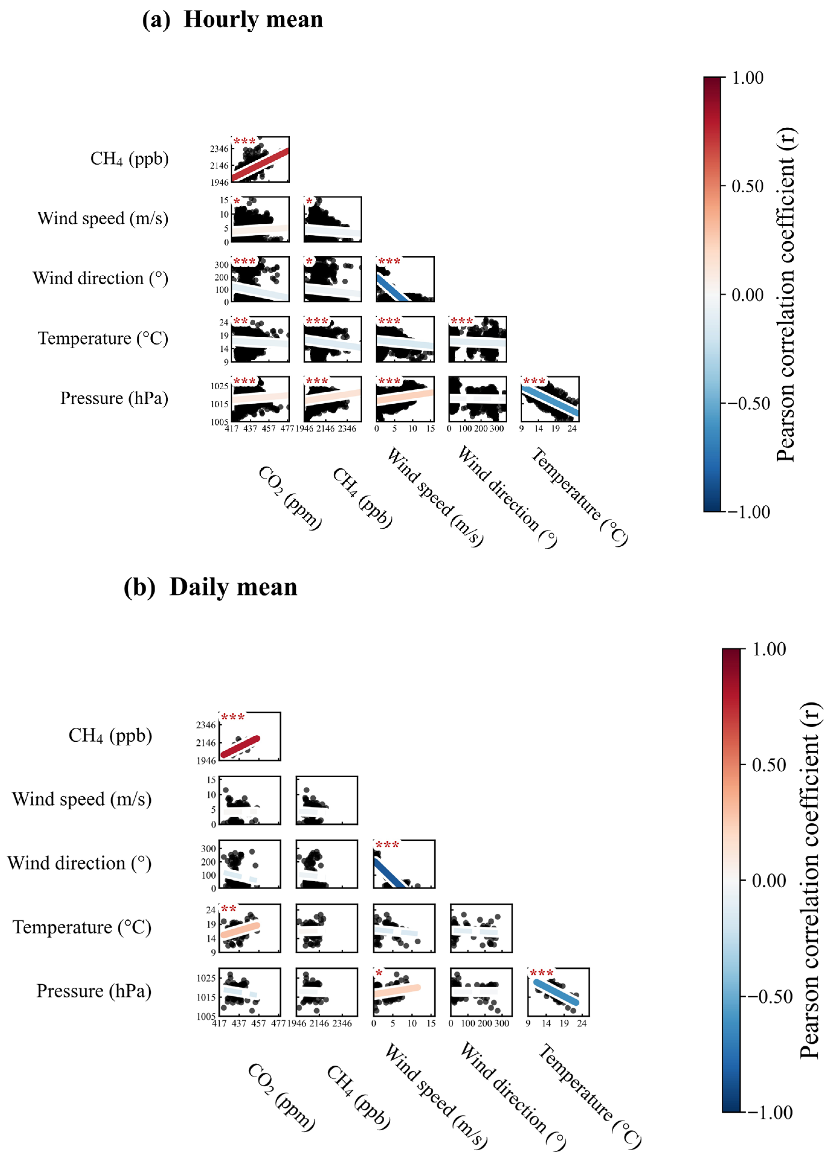
Common emission sources for CO₂ and CH₄ were reported by Ramachandran et al. [44,45,46]. At CDSS, the wind speed ranged from 0.10 to 15.48 m s⁻¹, with a mean of 4.05 ± 2.91 m s⁻¹ and 63.40% of winds originating from the 0–90° sector. The mean temperature during the study period was 16.56 ± 2.49 °C (range of 9.05–25.66 °C), and the average atmospheric pressure was 1017.63 ± 3.75 hPa (range of 1005.90–1029.10 hPa). The following correlations between CO₂ and CH₄ concentrations and meteorological variables at CDSS are illustrated in Figure 3: (1) Wind direction exhibited weak negative correlations with CO₂ (r = −0.11) and CH₄ (r = −0.05). (2) Correlations between wind speed and gas concentrations were not statistically significant for CO₂ (r = 0.06, p > 0.05) or CH₄ (r = −0.06, p > 0.05). (3) Atmospheric pressure showed a modest positive correlation with CH₄ concentrations (r = 0.14) but a negligible association with CO₂ concentrations (r = 0.09). (4) Temperature showed no significant correlation with CO₂ concentrations (r = −0.06) and a weak negative correlation with CH₄ concentrations (r = −0.13). The statistically significant covariance between CO₂ and CH₄ concentrations (r = 0.73, p < 0.001), coupled with negligible correlations between the concentrations of both gases and wind speed (r < 0.1), provides compelling evidence that the atmospheric methane and carbon dioxide in Hong Kong originate from shared emission sources. Moreover, the observed concentration dynamics are primarily influenced by regional-scale transport processes.

3.3. Source Distance Theory

Previous studies have demonstrated that under low wind speed conditions (<3 m s⁻¹), atmospheric processes are dominated by turbulent diffusion, which suppresses vertical mixing coefficients and effectively confines pollutants near the source region (<50 km), consistent with classical boundary-layer theory [47,48]. As wind speeds increase to the range of 3–8 m s⁻¹, a transition occurs wherein horizontal advection progressively overtakes vertical diffusion. During this regime, vertical turbulent mixing remains limited, while horizontal transport becomes more efficient, facilitating the regional-scale advection of pollutants over distances exceeding 200 km. This dynamic is consistent with wind-speed-dependent source attribution frameworks and highlights the potential for the long-range transport of externally derived pollutants into Hong Kong [49].

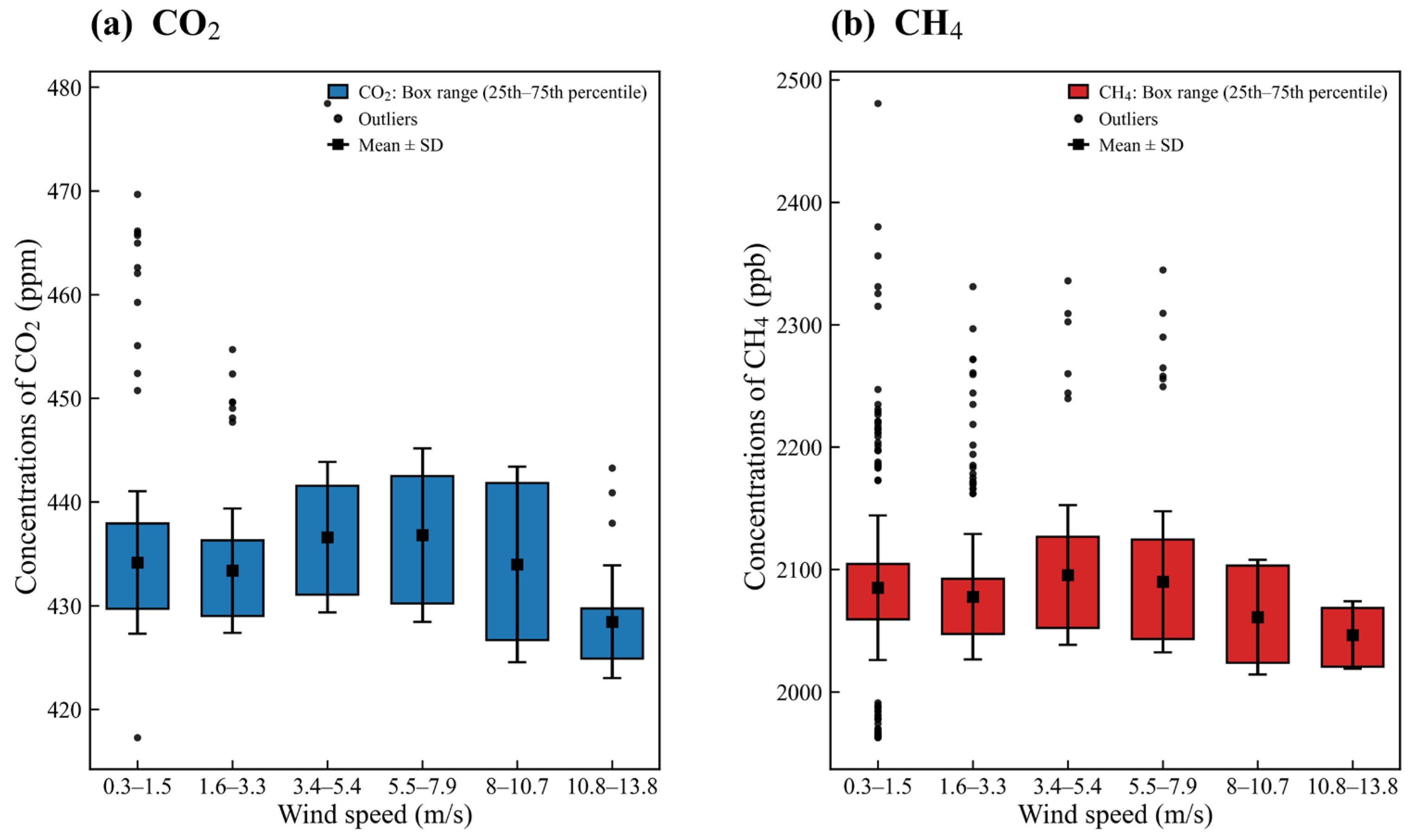
The analysis, stratified by Beaufort wind scale categories, revealed that CH₄ concentrations peaked at 2095.56 ± 57.05 ppb within the 3.4–5.4 m s⁻¹ wind speed range, while CO₂ reached its maximum concentration of 436.80 ± 8.35 ppm in the 5.5–7.9 m s⁻¹ interval (China Meteorological Administration, 2001; World Meteorological Organization, 2012 [50,51]) (Figure 4). These results provide strong evidence for the dominance of regional transport mechanisms under moderate wind conditions. At wind speeds exceeding 8 m s⁻¹, enhanced mechanical turbulence within the atmospheric boundary layer facilitates vertical mixing, thereby reducing near-surface accumulation of greenhouse gases. Collectively, these findings further substantiate that regional-scale transport is the principal driver of the CO₂ and CH₄ concentration dynamics in Hong Kong’s atmosphere.

3.4. Assessment of Transportation

3.4.1. Identification of Regional Transport Events and Provincial Spatial Weighting

The results from Section 3.1, Section 3.2 and Section 3.3 indicate that the wintertime CO₂ and CH₄ concentrations at CDSS are primarily governed by regional transport rather than local dispersion. The concentrations of these two gases covaried strongly (r = 0.73, p < 0.001), yet only weakly correlated with wind speed (|r| < 0.1), and both peaked under moderate winds (~3–8 m s⁻¹), conditions that favor horizontal advection. Building on this evidence, and consistent with the wind-speed–source-distance relationship in Section 3.3, we next analyzed 15 fixed-point air samples collected at CDSS during the same winter period to constrain the regional origins and sectoral contributions of GHGs.

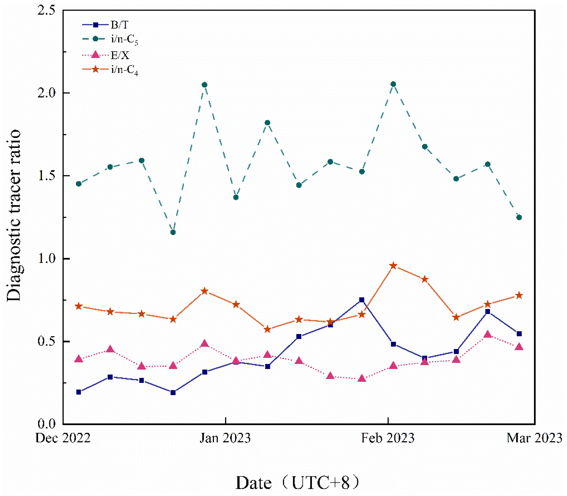
The ethylbenzene/m,p-xylene ratio (E/X) was used as a diagnostic indicator of photochemical aging because m,p-xylene is removed by OH more rapidly than ethylbenzene. An E/X > 0.33 signifies significantly aged air masses that are typically associated with regional/long-range transport, a criterion widely applied in previous studies [52,53]. In these manual samples, the ethylbenzene concentrations ranged from 39 to 240 ppt (mean ± SD: 113.07 ± 55.13 ppt) while the m,p-xylene concentrations varied from 111 to 613 ppt (mean ± SD: 288.13 ± 138.30 ppt). Based on the E/X threshold, 13 out of the 15 sampling episodes were classified as transport-dominated—5 in December, 3 in January, and 5 in February.

For these episodes, a total of 312 back trajectories were calculated, with 24 hourly initiation times per sampling day and each trajectory integrated 72 h backward. This trajectory ensemble formed the foundation for the subsequent spatial-weighting and sector-attribution analyses.

The frequency of trajectory passages over source provinces was statistically analyzed to derive spatially normalized weights $Q_j^{*}$ for each province as shown in Equation (1):

$$Q_j^{\mathrm{*}}={\displaystyle \frac{V_j}{{\sum }_{j=1}^m{V}_j}}\times 100\%$$

(1)

where $Q_j^{\mathrm{*}}$ is the provincial spatial weight for province j reported in percent (%), j indexes the different provinces (j = 1, …, m), m is the total number of provinces considered (dimensionless), V_j represents the trajectory passage count over province j (counts), and ${\sum }_{j=1}^m{V}_j$ is the total passage count across all provinces (counts).

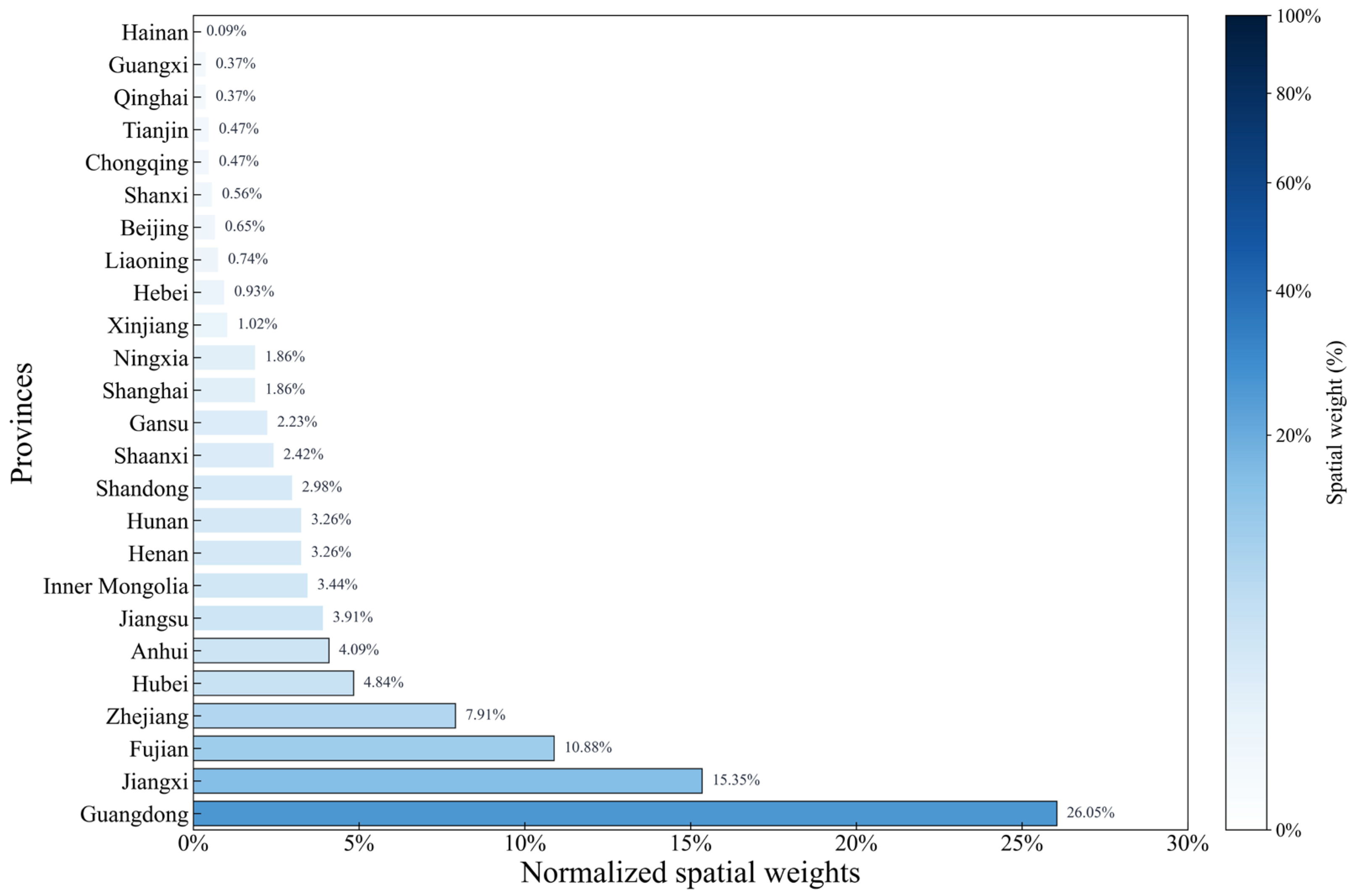
The normalized spatial weights are presented in Figure 5. Guangdong (26.05%), Jiangxi (15.35%), and Fujian (10.88%) emerged as the top three contributing provinces to Hong Kong GHG levels, while Guangxi (0.37%), Qinghai (0.37%), and Hainan (0.09%) contributed the least.

3.4.2. Source Attribution and Emission-Inventory Reconstruction

Considering the indicator evidence for regional-level attribution, the following source-specific hydrocarbon ratios were chosen to identify the transport episodes due to their relatively stable variation during regional transport.

(1)

Benzene/Toluene (B/T) Ratio

The B/T ratio was first used to separate solvent use- and vehicle emission-related plumes from combustion-dominated air masses. Published thresholds have delineated the following interpretation bands: B/T < 0.2 indicates solvent use, 0.2–1.0 indicates vehicle emissions, 1.0–1.5 reflects mixed combustion (e.g., biomass burning and incineration), and >1.5–2.2 indicates coal combustion [54,55,56,57,58]. Across 15 discrete samples, the benzene concentration ranged from 268 to 669 ppt (mean ± SD: 446 ± 141 ppt) and the toluene concentration was 555–1954 ppt (mean ± SD: 1145 ± 382 ppt). During regional transport episodes (n = 13), the B/T ratio was within the range of 0.2–1.0, implicating vehicle emissions with some influence from solvent use.

(2)

Isopentane/n-Pentane (i/n-C₅) Ratio

This ratio differentiates combustion from mobile and evaporative signatures: 0.56–0.80 typifies coal combustion, 0.82–1.10 indicates oil and gas operations or ship exhaust, 2.2–3.8 is characteristic of vehicle emissions (exhaust), and 1.50–4.60 indicates fuel evaporation [36,59,60,61,62,63,64,65,66]. The isopentane concentration ranged from 160 to 575 ppt (372 ± 139 ppt) and the n-pentane concentration was 110–396 ppt (240 ± 94 ppt). In the transport episodes, i/n-C₅ = 1.25–2.05, which is above the oil and gas operations/ship band but below the canonical vehicle emissions band, indicating the dominance of vehicle emissions (with gasoline evaporation) with potential minor contributions from oil and gas operations (including ship exhaust) when the ratio is near the lower bound.

(3)

Isobutane/n-Butane (i/n-C4) Ratio

Sector discrimination was further refined using the i/n-C₄ ratio, where a ratio of 0.2–0.3 reflects vehicle emissions (exhaust), ≈0.46 indicates Liquefied Petroleum Gas (LPG) emissions, and 0.6–1.0 is diagnostic of natural gas emissions [36,62,67,68]. The isobutane concentration was measured to be 305–962 ppt (617 ± 184 ppt) and the n-butane concentration was 481–1389 ppt (884 ± 298 ppt); all transport episodes fell within the range of 0.6–1.0, identifying natural gas emissions as the predominant contributor (Figure 6).

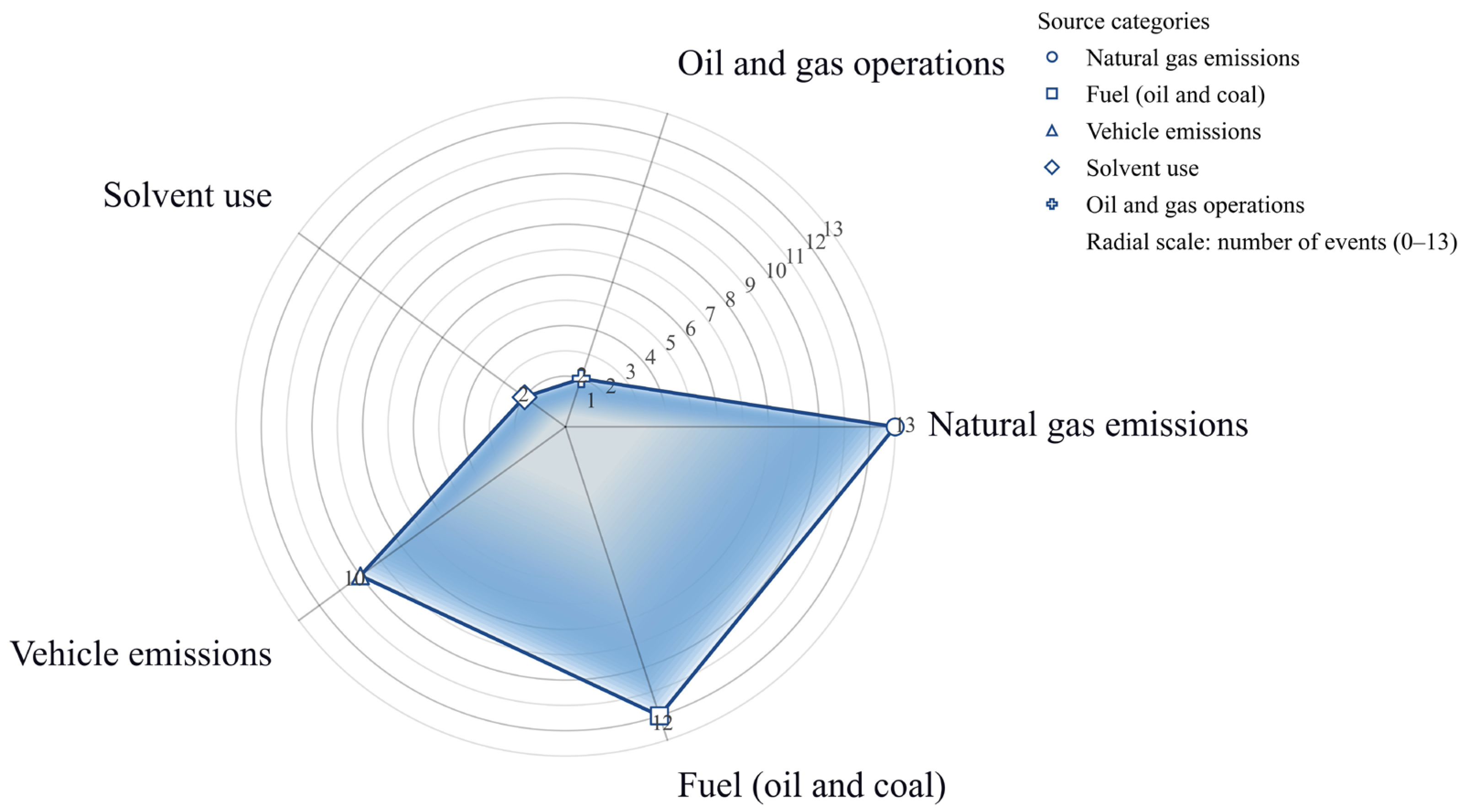
Source attribution based on diagnostic hydrocarbon ratios (B/T, i/n-C₅, and i/n-C₄) during regional transport episodes revealed five predominant contributing sectors to greenhouse-gas-associated co-emissions in Hong Kong: (1) natural gas emissions, (2) fuel combustion (oil and coal), (3) vehicle emissions, (4) solvent use, and (5) oil and gas operations. Among the 13 identified transport events, natural gas emissions were implicated in all events (13/13), followed by fuel combustion (12/13) and vehicular emissions (10/13), whereas solvent use and oil and gas operations were each indicated in 2 of the 13 episodes.

The Multi-resolution Emission Inventory for China (MEIC) was re-constructed from 52 industrial sectors into five consolidated source categories following this classification scheme. The mapping between these five categories and the MEIC sectors is provided in

Table 2. Mapping of the major sources in re-constructed inventory with the high-resolution emission inventory (MEIC sectors).

Major Source in Reconstructed Inventory	Sectors in the High-Resolution Inventory (MEIC)
Natural gas emissions	Gas works, gasification plants, liquefaction/regasification plants, pipeline transport
Fuel (oil and coal)	Oil refineries, coal liquefaction, GTL plants
Vehicle emissions	Cars, light-duty trucks, buses, heavy-duty trucks, motorcycles, other fleets
Solvent use	Chemical, pulp and paper, wood product, textile and leather industries
Oil and gas operations	Oil and gas extraction, transport equipment *, domestic navigation

Note: * Transport equipment refers to operational/functional aspects directly related to the oil and gas supply chain (e.g., storage, transportation, and refueling).

.

For the 13 regional-transport events identified during the winter sampling campaign—5 in December, 3 in January, and 5 in February—monthly sampling weights were derived by dividing the number of events in each month by the total number of events (n = 13).

These weights, defined in Equation (2), were applied to the preprocessed provincial monthly emission totals across all five source categories. This temporal weighting approach enabled the calculation of representative provincial-scale aggregated emissions that reflect the seasonality of regional transport influences.

$$E_{win,j,c}={\displaystyle \frac{5}{13}}\times E_{Dec,j,c}+{\displaystyle \frac{3}{13}}\times E_{Jan,j,c}+{\displaystyle \frac{5}{13}}\times E_{Feb,j,c}$$

(2)

where c denotes the source category (vehicle emissions, fuel (oil/coal), solvent use, oil and gas operations, natural gas emissions); j indexes the different provinces (j = 1,…, m); E_win,j,c is the winter-weighted emission of species CO₂ for province j and category c (unit: kt CO₂); E_Dec,j,c, E_Jan,j,c, and E_Feb,j,c are the monthly emissions in December, January, and February for source category c in province j (unit: kt CO₂), respectively; the numerical coefficients 5/13, 3/13, and 5/13 are the monthly event weights derived from the counts of identified transport events (dimensionless).

Following this province-level temporal aggregation, the relative contributions of the five source categories were quantified based on their diagnostic-ratio occurrence frequencies across the 13 transport events. Using 39 diagnostic ratio data points, the percentage contribution of each source category was determined via Equation (3):

$$W_{ind,c}={\displaystyle \frac{F_c}{\sum _{c=1}^5{F}_C}}\times 100\%$$

(3)

where c denotes the source category (c = 1, …, 5) (vehicle emissions, fuel (oil/coal), solvent use, oil and gas operations, natural gas emissions); F_c is the occurrence frequency assigned to category c based on the diagnostic-ratio indications across the 13 transport events (counts); $\sum _{c=1}^5{F}_C$ is the total frequency across all five categories (counts); and $W_{ind,c}$ is the sectoral weighting for category c, reported in percent (%).

The resulting distribution (Figure 7) indicates that natural gas was identified in 33.33% of the source-category occurrences across the 13 events, followed by fuel combustion (30.77%), vehicular emissions (25.64%), and solvent use and oil and gas operations (5.13% each).

3.4.3. Quantifying Provincial and Sector Contributions to Cross-Regional GHG Transport

Based on the provincial spatial weights $Q_j^{\mathrm{*}}$ (Section 3.4.1) and the source-type weights W_ind,c and the winter-weighted emissions E_win,j,c from the reconstructed province–source inventory (Section 3.4.2), we constructed an integrated framework to quantify the contributions of province–source-category combinations to cross-regional GHG transport into Hong Kong. Equation (4) combines $Q_j^{\mathrm{*}}$, W_ind,c, and E_win,j,c with $Q_j^{\mathrm{*}}$, obtained from 72 h back-trajectory frequency statistics (Equation (1)), E_win,j,c calculated from the reclassified MEIC inventory using monthly event weights (Equation (2)), and W_ind,c derived from the occurrence frequency of diagnostic hydrocarbon ratios across the 13 identified transport events (Equation (3)) to estimate the total contribution ${\phi }_{j,c}$ for each province–source-category combination.

$${\phi }_{j,c}=Q_j^{*}\times W_{ind,c}\times E_{win,j,c}$$

(4)

In this expression, ${\phi }_{j,c}$ represents the total contribution of source category c from province j to Hong Kong (kt CO₂), $Q_j^{*}$ is the spatial-normalization weight for province j (%), E_win,j,c is the winter-weighted emission from source category c in province j (kt CO₂), and W_ind,c indicates the sector impact factor for source category c (%).

The three variables in Equation (4) are independent of each other. $Q_j^{*}$ reflects the transport frequency (72 h trajectory counts), $W_{ind,c}$ reflects the diagnostic-ratio occurrence across events (chemical diagnostics), and $E_{win,j,c}$ reflects the activity magnitude from the winter-weighted province–sector inventory. Each factor is normalized before combination, which minimizes first-order covariance by design.

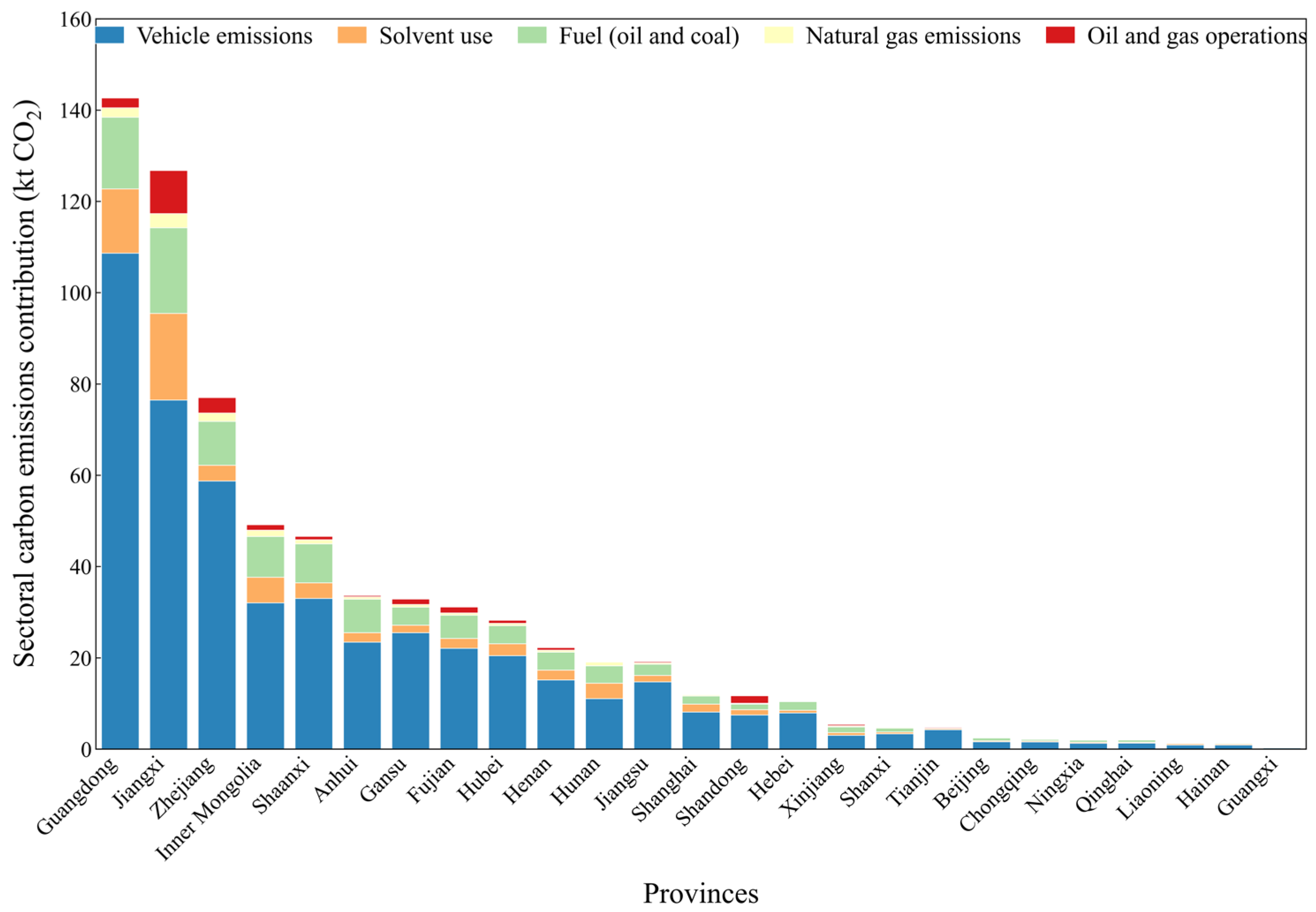
Based on a systematic assessment of 13 wintertime regional-transport events, province-level contributions to cross-regional industrial CO₂ transport into Hong Kong exhibited pronounced spatial heterogeneity (Figure 8).

Guangdong, Jiangxi, and Zhejiang were the top three contributors, with estimated emissions of 142.67 kt CO₂, 126.78 kt CO₂, and 77.02 kt CO₂, respectively. By contrast, Liaoning (1.38 kt CO₂), Hainan (1.37 kt CO₂), and Guangxi (0.36 kt CO₂) contributed the least. This spatial distribution reflects disparities in provincial emission intensities as well as the complexity of cross-regional transport efficiency.

Guangdong contributed the largest share of CO₂, with all five source categories ranking among the top three nationwide. Vehicle emissions dominated (108.63 kt CO₂), followed by fuel combustion (oil and coal) (15.68 kt CO₂), solvent use (14.12 kt CO₂), oil and gas operations (2.17 kt CO₂), and natural gas emissions (2.07 kt CO₂). This high-intensity emissions profile is consistent with the Pearl River Delta (PRD), where more than 20 million registered vehicles sustain continuous mobile-source emissions, and dense port–shipping networks—particularly in Shenzhen and Guangzhou—amplify transport-related outputs. Meteorologically, Guangdong’s location south of the Nanling Mountains places it within the prevailing winter northeasterly monsoon corridor. Under anticyclonic conditions, suppressed boundary-layer heights favor near-surface pollutant accumulation, while persistent northerly flows facilitate the low-level advection of polluted air masses toward Hong Kong.

Jiangxi ranked second in total CO₂ contributions. Solvent use (18.99 kt CO₂) and oil and gas operations (9.45 kt CO₂) in Jiangxi represented the highest provincial contributions for these categories. Additional contributions included vehicle emissions (76.47 kt CO₂), fuel combustion (oil and coal) (18.77 kt CO₂), and natural gas emissions (3.10 kt CO₂), all ranking among the top three provincially. This sectoral profile reflects extensive petrochemical and pharmaceutical clusters in northern and southern Jiangxi, including solvent-intensive operations at the Jiujiang Petrochemical Base and VOC-emitting processes in Yichun’s pharmaceutical sector. Topographically, the northern foothills of the Nanling Mountains can inhibit cold-air penetration from the north, enhancing boundary-layer stability and prolonging pollutant residence times. Under favorable synoptic conditions, however, pollutant-laden air masses may traverse these barriers and be advected southwestward via low-level flow, forming effective short-range transport pathways that impact Hong Kong’s urban core.

Zhejiang Province ranked third in total industrial CO₂ contributions, with emissions dominated by vehicle emissions (58.74 kt CO₂), followed by fuel combustion (oil and coal) (9.60 kt CO₂), solvent use (3.45 kt CO₂), oil and gas operations (3.38 kt CO₂), and natural gas emissions (1.85 kt CO₂). This source distribution is broadly consistent with provincial source-control strategies. At the Ningbo–Zhoushan Port, the over 200,000 freight-vehicle movements per day generate substantial transport-related emissions, while international shipping remains a dominant contributor to NO_x emissions—Ningbo Port alone released 140,310 tonnes of NO_x in 2019, accounting for 31.6% of the total emissions from 17 ports in the Yangtze River Delta region [69]. Seasonal easterly winds entrain coastal pollutants southwestward, and the high marine humidity enhances aqueous-phase chemical processes, promoting secondary pollution formation in downwind areas.

Despite their greater source–receptor distances, the Inner Mongolia Autonomous Region (49.15 kt CO₂) and Shaanxi Province (46.60 kt CO₂) contributed more than many eastern provinces. In both regions, emissions were dominated by fuel combustion (oil and coal) (Inner Mongolia: 8.94 kt CO₂; Shaanxi: 8.52 kt CO₂) and vehicle emissions (Inner Mongolia: 32.03 kt CO₂; Shaanxi: 33.01 kt CO₂), consistent with the widespread winter coal-based heating in the Yellow River midstream energy corridor. Long-range pollutant transport from these inland regions primarily occurs within the mid-tropospheric westerlies (3000–5000 m), where high horizontal wind speeds (>15 m s⁻¹) and low vertical diffusion coefficients (K_z < 2 m² s⁻¹) minimize dilution. Trajectory analyses suggest that air masses traveling along northwest–southeast pathways can maintain elevated pollutant concentrations over distances approaching 2000 km, reaching Hong Kong via subsidence-induced fumigation in coastal South China.

Among the low-contribution regions, the Guangxi Zhuang Autonomous Region exhibited the lowest total of 0.36 kt CO₂, primarily from vehicle emissions (0.26 kt CO₂), with all source categories showing very low emission intensities. This reflects the relatively underdeveloped industrial structure in western Guangxi. Moreover, atmospheric transport is constrained by unstable flow patterns: the western Pearl River Estuary corridor is frequently influenced by peripheral circulations associated with South China Sea tropical systems during winter. Under anomalously strong cross-equatorial flows, the low-level wind direction may shift by over 90°, severely disrupting directional transport toward Hong Kong.

Hainan Province contributed a total of 1.37 kt CO₂, with negligible input from oil and gas operations (0.01 kt CO₂) and solvent use (0.24 kt CO₂), owing to its limited emission base. Critically, pollutants from Hainan are primarily driven southward by the northeast monsoon during November–February, directing emissions into the South China Sea. Simultaneously, strong solar radiation enhances photochemical degradation, further limiting its downwind influence.

Liaoning Province contributed 1.38 kt CO₂, mainly from vehicle emissions (0.92 kt CO₂), solvent use (0.26 kt CO₂), and fuel combustion (oil and coal) (0.12 kt CO₂). This limited cross-regional impact is primarily attributed to persistent wintertime temperature inversions over Liaodong Bay, which establish strong stable layers that suppress vertical turbulence, inhibit the vertical injection of surface pollutants, and restrict their entrainment into the free troposphere.

Overall, the observed regional patterns delineate a three-tiered spatial hierarchy governing wintertime GHG transport to Hong Kong, shaped by the interplay between emission intensities and atmospheric transport mechanisms.

The primary tier includes Guangdong and Jiangxi. In winter, the East Asian monsoon establishes a near-surface transport corridor oriented along a northeasterly direction toward Hong Kong, creating a favorable spatial alignment between Guangdong/Jiangxi and the receptor. This corridor exhibits high frequency and sufficient residence time, while the shallow winter boundary layer further minimizes interference during transport. Regarding industrial structure, Guangdong demonstrates dominant contributions from transportation and port activities, whereas Jiangxi shows stronger influences from solvent- and oil/gas-related emissions. These features align with the tracer ratio fingerprints used to identify dominant transport periods. Nocturnal land–sea-breeze circulation helps sustain low-level coastal advection. The synergistic effects of corridor frequency, shallow boundary layer, and source–tracer fingerprint consistency collectively explain their persistent dominance in driving Hong Kong’s greenhouse gas variations during winter.

The secondary tier consists of coastal Zhejiang, which is characterized by significant port and coastal transportation activities, and exhibits a pronounced combustion emission signal. During winter, the continental monsoon in this region generates a “backflow” pattern behind cold fronts, which facilitates the southward transport of easterly airflow near 850 hPa along the coastline, serving as an efficient secondary transport pathway. Combustion plumes co-emitted with CO₂/CH₄ are effectively transported through this corridor. Consequently, the impact of coastal Zhejiang on Hong Kong is secondary to that of the Guangdong–Jiangxi segment, as it involves longer transport distances and more complex air–sea exchange processes, resulting in a lower overall contribution compared with the dominant tier.

The tertiary tier encompasses northern inland provinces such as Shaanxi and Inner Mongolia. Emissions in northern inland areas during winter are predominantly due to fuel combustion (oil and coal) and transportation-related activities. However, their influence on the receptor region (e.g., Hong Kong) is significantly attenuated due to two primary factors: firstly, the long source–receptor distance (typically exceeding 1000 km) results in substantial atmospheric dilution and deposition during transport. Divergent large-scale circulation patterns (e.g., prevailing westerlies, monsoon shifts) often divert emissions away from the direct pathway to Hong Kong. Second, high-altitude emissions (e.g., from industrial stacks or elevated sources) can be lifted into the middle troposphere (~700–500 hPa) by frontal systems or convection. At these altitudes, reduced vertical mixing and weaker scavenging by precipitation allow pollutants to undergo long-range advection (e.g., across the Yangtze River Delta or South China). Subsequent subsidence over southern China, combined with vertical mixing (e.g., daytime turbulence and nocturnal drainage flows), may reintroduce pollutants into the boundary layer, where local winds (e.g., northeasterly monsoon flows) can transport them toward Hong Kong.

Minimal contributions were observed from Guangxi, Hainan, and Liaoning. These regions are characterized by weak signals, low arrival frequencies, corridor misalignment, and enhanced dilution. Source regions not geometrically aligned with Hong Kong (e.g., Guangxi and Hainan) frequently experience offshore southward or southwesterly diversion, while more northern inland sources (e.g., Liaoning) primarily follow southeasterly pathways discharging into the Yellow Sea/East China Sea. These transport routes feature short regional transit windows and strong dilution, resulting in intermittent, low-probability impacts on Hong Kong. Additionally, the industrial structure and activity intensity in these regions are weaker compared with the Pearl River Delta and Jiangxi industrial belt, and their tracer fingerprints do not match those of dominant contributors. These factors collectively account for the negligible contribution of this tier to Hong Kong under the winter framework.

3.5. Uncertainty Analysis

As specified in Equation (4), the contribution estimator integrates three components derived from distinct data streams: province-level spatial weights $Q_j^{*}$ (normalized 72 h HYSPLIT back-trajectory frequencies during identified transport episodes), source-type weights $W_{ind,c}$ (literature-based diagnostic-ratio occurrences), and winter-weighted emissions ${ E}_{win,j,c}$ (restructured province–sector inventory). Uncertainty may arise from transport representation (meteorological resolution, release height, and boundary-crossing statistics), from potential overlap of diagnostic thresholds under aging or source mixing, and from inventory quality and the aggregation of fine sectors into the study’s five categories. To limit covariance artifacts in the multiplicative form, the three factors were estimated via separate procedures and internally normalized on their own supports (e.g., ${\sum }_j{Q}_j^{*}=1$ and ${\sum }_c{W}_{ind,c}=1$), which constrains cross-term co-scaling and prevents the reuse of common signals; as a result, $Q_j^{*}$ encodes corridor frequency/residence, $W_{ind,c}$ encodes source taxonomy, and $E_{win,j,c}$ encodes magnitude. Any residual covariance is expected to reflect genuine co-variation (e.g., a synoptic corridor coincident with seasonal emissions) and is assessed empirically below.

To assess the methodological framework and uncertainties, we validated Equation (4) using two experiments: One-At-a-Time (OAT) perturbation analysis and Leave-One-Event-Out (LOEO) analysis. The OAT method tests the robustness of provincial/sectoral emission contributions to variations in key inputs (spatial weights, source category weights, and emission inventory data), while LOEO analysis evaluates sample size effects. Percentage points (pp) denote absolute changes on a 0–100% scale (e.g., 20.0% → 20.7% = +0.7 pp). In OAT analysis, each input factor is individually perturbed (±10% or ±20%) while the others are held constant, including spatial weights ($Q_j^{*}$) by province (j), source category weights ($W_{ind,c}$), and winter emissions ($E_{win,j,c}$) organized by province and category. After each perturbation, the model recalculates, and provincial/sectoral contributions are compared with baseline results. Across 264 OAT scenarios (±10% and ±20%), the sectoral ranking never changed (0/264), and the set of dominant provinces (Guangdong, Jiangxi, and Zhejiang) remained unchanged in all cases. The typical absolute changes were small: for ±10% perturbations, the provincial contributions showed a median maximum change of 0.097 pp (upper quartile: 0.394 pp; max: 1.674 pp) while the sectoral contributions were calculated to be 0.013 pp (upper quartile: 0.036 pp; max: 2.881 pp); for ±20% perturbations, these values increased to 0.193 pp (provincial) and 0.025 pp (sectoral), with upper quartiles of 0.791 and 0.072 pp, respectively, and maxima of 3.420 and 4.881 pp. Rank flips, when they occurred, were limited to mid-tier provinces with similar baseline shares and did not affect the top three provinces while the sectoral order was entirely invariant.

The LOEO analysis systematically removed each of the 13 identified regional transport events (after temporal alignment of online and sampling data) and recalculated the attribution model. For each excluded event, provincial and sectoral contributions are recomputed and compared against baseline values to assess result stability. Consistent with the OAT results, LOEO analysis found the same core findings. The median of the per-scenario maximum provincial absolute changes was 0.141 percentage points (pp), with the largest observed change being 1.043 pp (event e4, Jiangxi). The dominant provinces (Guangdong, Jiangxi, and Zhejiang) maintained their rankings in all 13 scenarios, confirming that the leading contributors were not determined by any single transport event. The LOEO procedure also evaluated the sectoral contribution stability. For each of the 13 single-event exclusion scenarios, the contributions from the five major emission source categories—vehicle emissions, fuel (oil and coal), solvent use, oil and gas production, and natural gas emissions—were recalculated and compared against the baseline values. The sectoral contributions exhibited minimal variations across scenarios. Vehicle emissions (baseline ~70.03%) remained the largest contributor in all cases. The ranking of the top-contributing sectors was unaffected by any single event exclusion: fuel (oil and coal) (~14.67%) remained second and solvent use (~9.73%) remained third. For the two least significant categories—oil and gas operations (~3.47%) and natural gas emissions (~2.10%)—the exclusion of specific events led to larger relative changes due to small denominators and a pairwise rank swap in two scenarios. However, the absolute shifts remained small and did not affect the major sector rankings.

Overall, ±20% perturbations were more likely to trigger rank flips than ±10% perturbations. Notably, these flips were concentrated in mid-tier provinces with similar baseline shares, while dominant provinces rarely experienced them. This suggests that within reasonable input uncertainty ranges, the dominant pattern remains robust, and the overall hierarchical structure is preserved. In particular, the sectoral order was unchanged in all 264 OAT scenarios, and the top three provinces (Guangdong, Jiangxi, and Zhejiang) remained consistent across all OAT and LOEO tests. Typical absolute provincial changes stayed well below 1 pp even under ±20% stress tests.

4. Conclusions

This study presents a transparent, observation-driven, event-based framework for attributing cross-boundary CO₂ and CH₄ transport to Hong Kong at province-sector resolution, with limited reliance on numerical models. The framework uses a simple, linked workflow that turns routine measurements into policy-ready source shares: diagnostic VOC ratios (e.g., E/X) identify transport-dominated hours at the event scale, tying the analysis window to atmospheric processes rather than fixed calendar periods; 72 h back-trajectory counts are summarized as normalized provincial spatial weights, a traceable indicator of corridor frequency and air-mass residence that requires no tuning of chemical mechanisms; and a reconstructed province–sector inventory is matched to the diagnostic scheme using literature-based ratio thresholds and clear aggregation rules, preserving interpretability from tracer signal to emission category.

Applied to winter 2022, the analysis indicates that Hong Kong’s GHG variability was largely transport-driven. A coherent three-tier provincial pattern emerged: Guangdong was the dominant external contributor (≈20%), followed by Jiangxi (≈18%) and Zhejiang (≈11%), whereas the contributions of Guangxi, Qinghai, and Hainan were negligible. By sector, the regional contributions were dominated by motor-vehicle/transport emissions (≈70%), followed by fuel (oil and coal) combustion (≈15%) and solvent use (≈10%); oil and gas operations and natural gas emissions were minor but distinct categories, with solvent use notably elevated in Jiangxi. In practical terms, the framework turns observations into actionable province–sector shares with modest data and computational requirements, enabling rapid screening, tracking of seasonal shifts in upwind influence, and prioritization of corridor-focused measures such as vehicle and solvent controls and port transport interventions along winter monsoon pathways.

References

1. Harde, H. Radiation and heat transfer in the atmosphere: A comprehensive approach on a molecular basis. Int. J. Atmos. Sci. 2013, 2013, 1–26. [Google Scholar] [CrossRef]
2. World Meteorological Organization (WMO). WMO Greenhouse Gas Bulletin No. 19: The State of Greenhouse Gases in the Atmosphere Based on Global Observations Through 2022; World Meteorological Organization: Geneva, Switzerland, 2023; Available online: https://public.wmo.int/ (accessed on 10 January 2025).
3. Filonchyk, M.; Peterson, M.P.; Zhang, L.; Hurynovich, V.; He, Y. Greenhouse gases emissions and global climate change: Examining the influence of CO2, CH4, and N2O. Sci. Total Environ. 2024, 935, 173359. [Google Scholar] [CrossRef] [PubMed]
4. Harriss, R.C.; Sebacher, D.I.; Day, F.P. Methane flux in the Great Dismal Swamp. Nature 1982, 297, 673–674. [Google Scholar] [CrossRef]
5. Zhang, Q.; Zheng, Y.; Tong, D.; Shao, M.; Wang, S.; Zhang, Y.; Xu, X.; Wang, J.; He, H.; Liu, W.; et al. Drivers of improved PM2.5 air quality in China from 2013 to 2017. Proc. Natl. Acad. Sci. USA 2019, 116, 24463–24469. [Google Scholar] [CrossRef]
6. Qian, H.; Xu, S.; Cao, J.; Ren, F.; Wei, W.; Meng, J.; Wu, L. Air pollution reduction and climate co-benefits in China’s industries. Nat. Sustain. 2021, 4, 417–425. [Google Scholar] [CrossRef]
7. Shao, T.; Wang, P.; Yu, W.; Gao, Y.; Zhu, S.; Zhang, Y.; Hu, D.; Zhang, B.; Zhang, H. Drivers of alleviated PM2.5 and O3 concentrations in China from 2013 to 2020. Resour. Conserv. Recycl. 2023, 197, 107110. [Google Scholar] [CrossRef]
8. Wang, C.; Deng, H.M.; Guo, K.D.; Liu, Y. Research Progress on Cooperative Governance of Greenhouse Gases and Air Pollutants. Chin. J. Environ. Manag. 2020, 12, 5–12. [Google Scholar] [CrossRef]
9. Balcombe, P.; Brandon, N.P.; Hawkes, A.D. Characterising the distribution of methane and carbon dioxide emissions from the natural gas supply chain. J. Clean. Prod. 2018, 172, 2019–2032. [Google Scholar] [CrossRef]
10. Harrison, B.P.; Gao, S.; Gonzales, M.; Thao, T.; Bischak, E.; Ghezzehei, T.A.; Berhe, A.A.; Diaz, G.; Ryals, R.A. Dairy manure co-composting with wood biochar plays a critical role in meeting global methane goals. Environ. Sci. Technol. 2022, 56, 10987–10996. [Google Scholar] [CrossRef]
11. Salas-Rabaza, J.A.; Andrade, J.L.; Us-Santamaría, R.; Morales-Rico, P.; Mayora, G.; Aguirre, F.J.; Fecci-Machuca, V.; Gade-Palma, E.M.; Thalasso, F. Impacts of leaks and gas accumulation on closed chamber methods for measuring methane and carbon dioxide fluxes from tree stems. Sci. Total Environ. 2023, 904, 166358. [Google Scholar] [CrossRef]
12. Akpasi, S.O.; Akpan, J.S.; Amune, U.O.; Olaseinde, A.A.; Kiambi, S.L. Methane advances: Trends and summary from selected studies. Methane 2024, 3, 276–313. [Google Scholar] [CrossRef]
13. Ma, Y.Y.; Zhou, Y.; Sheng, L.F.; Wang, W.C.; Yu, J.Z. Circulation clustering characteristics causing air pollution in Hong Kong and their impact on fine particulate matter. Geochimica 2021, 50, 22–35. [Google Scholar] [CrossRef]
14. Wang, H.; Lyu, X.; Guo, H.; Wang, Y.; Zou, S.; Ling, Z.; Wang, X.; Jiang, F.; Zeren, Y.; Pan, W.; et al. Ozone pollution around a coastal region of South China Sea: Interaction between marine and continental air. Atmos. Chem. Phys. 2018, 18, 4277–4295. [Google Scholar] [CrossRef]
15. Jianghong, H.; Yue, L.; Ying, Z.; Qinyu, C.; Xiuyong, Z.; Dongsheng, C. The ozone concentration and changes in the sensitivity of its formation in Guangdong–Hong Kong–Macao Greater Bay Area (GBA) from a carbon neutral perspective. J. Resour. Ecol. 2024, 15, 204–213. [Google Scholar] [CrossRef]
16. Talbot, C.; Augustin, P.; Leroy, C.; Willart, V.; Delbarre, H.; Khomenko, G. Impact of a sea breeze on the boundary-layer dynamics and the atmospheric stratification in a coastal area of the North Sea. Bound.-Layer Meteorol. 2007, 125, 133–154. [Google Scholar] [CrossRef]
17. Jiménez, P.A.; de Arellano, J.V.-G.; Dudhia, J.; Bosveld, F.C. Role of synoptic- and meso-scales on the evolution of the boundary-layer wind profile over a coastal region: The near-coast diurnal acceleration. Meteorol. Atmos. Phys. 2015, 128, 39–56. [Google Scholar] [CrossRef]
18. Pipalatkar, P.; Khaparde, V.V.; Gajghate, D.G.; Bawase, M.A. Source apportionment of PM2.5 using a CMB model for a centrally located Indian city. Aerosol Air Qual. Res. 2014, 14, 1089–1099. [Google Scholar] [CrossRef]
19. Jain, S.; Sharma, S.K.; Choudhary, N.; Masiwal, R.; Saxena, M.; Sharma, A.; Mandal, T.K.; Gupta, A.; Gupta, N.C.; Sharma, C. Chemical characteristics and source apportionment of PM2.5 using PCA/APCS, UNMIX, and PMF at an urban site of Delhi, India. Environ. Sci. Pollut. Res. 2017, 24, 14637–14656. [Google Scholar] [CrossRef]
20. Li, X.; Hussain, S.A.; Sobri, S.; Md Said, M.S. Overviewing the air quality models on air pollution in Sichuan Basin, China. Chemosphere 2021, 271, 129502. [Google Scholar] [CrossRef]
21. Yuan, Q.; Zhang, Z.; Chen, Y.; Hui, L.; Wang, M.; Xia, M.; Zou, Z.; Wei, W.; Ho, K.F.; Wang, Z.; et al. Origin and transformation of volatile organic compounds at a regional background site in Hong Kong: Varied photochemical processes from different source regions. Sci. Total Environ. 2024, 908, 168316. [Google Scholar] [CrossRef]
22. Draxler, R.R.; Hess, G.D. An overview of the HYSPLIT_4 modelling system for trajectories, dispersion, and deposition. Aust. Meteorol. Mag. 1998, 47, 295–308. [Google Scholar]
23. Wong, D.C.; Pleim, J.; Mathur, R.; Binkowski, F.; Otte, T.; Gilliam, R.; Pouliot, G.; Xiu, A.; Young, J.O.; Kang, D. WRF-CMAQ two-way coupled system with aerosol feedback: Software development and preliminary results. Geosci. Model Dev. 2012, 5, 299–312. [Google Scholar] [CrossRef]
24. Gao, Z.; Zhou, X. A review of the CAMx, CMAQ, WRF-Chem and NAQPMS models: Application, evaluation and uncertainty factors. Environ. Pollut. 2024, 343, 123183. [Google Scholar] [CrossRef] [PubMed]
25. Wong, Y.K.; Huang, X.H.H.; Cheng, Y.Y.; Yu, J.Z. Estimating primary vehicular emission contributions to PM2.5 using the chemical mass balance model: Accounting for gas–particle partitioning of organic aerosols and oxidation degradation of hopanes. Environ. Pollut. 2021, 291, 118131. [Google Scholar] [CrossRef]
26. Tan, Y.; Han, S.; Chen, Y.; Zhang, Z.; Li, H.; Li, W.; Yuan, Q.; Li, X.; Wang, T.; Lee, S. Characteristics and source apportionment of volatile organic compounds (VOCs) at a coastal site in Hong Kong. Sci. Total Environ. 2021, 777, 146241. [Google Scholar] [CrossRef]
27. Wang, F.; Ho, S.S.H.; Man, C.L.; Qu, L.; Wang, Z.; Ning, Z.; Ho, K.F. Characteristics and sources of oxygenated VOCs in Hong Kong: Implications for ozone formation. Sci. Total Environ. 2024, 912, 169156. [Google Scholar] [CrossRef]
28. Crosson, E.R. A cavity ring-down analyzer for measuring atmospheric levels of methane, carbon dioxide, and water vapor. Appl. Phys. B 2008, 92, 403–408. [Google Scholar] [CrossRef]
29. Chen, H.; Winderlich, J.; Gerbig, C.; Hoefer, A.; Rella, C.W.; Crosson, E.R.; Van Pelt, A.D.; Steinbach, J.; Kolle, O.; Beck, V.; et al. High-accuracy continuous airborne measurements of greenhouse gases (CO2 and CH4) using the cavity ring-down spectroscopy (CRDS) technique. Atmos. Meas. Tech. 2010, 3, 375–386. [Google Scholar] [CrossRef]
30. Blake, D.R.; Smith, T.W.; Chen, T.-Y.; Whipple, W.J.; Rowland, F.S. Effects of biomass burning on summertime nonmethane hydrocarbon concentrations in the Canadian wetlands. J. Geophys. Res. Atmos. 1994, 99, 1699–1719. [Google Scholar] [CrossRef]
31. Horst, T.W.; Vogt, R.; Oncley, S.P. Measurements of flow distortion within the IRGASON integrated sonic anemometer and CO2/H2O gas analyzer. Bound.-Layer Meteorol. 2016, 160, 1–15. [Google Scholar] [CrossRef]
32. Zhou, X.; Yang, Q.; Zhen, X.; Li, Y.; Hao, G.; Shen, H.; Gao, T.; Sun, Y.; Zheng, N. Recovery of the three-dimensional wind and sonic temperature data from a physically deformed sonic anemometer. Atmos. Meas. Tech. 2018, 11, 5981–6002. [Google Scholar] [CrossRef]
33. World Data Centre for Greenhouse Gases (WDCGG). WMO GAW World Data Centre for Greenhouse Gases. Available online: https://gaw.kishou.go.jp/ (accessed on 1 June 2025).
34. Li, K.; Jacob, D.J.; Liao, H.; Shen, L.; Zhang, Q.; Bates, K.H. Anthropogenic drivers of 2013–2017 trends in summer surface ozone in China. Proc. Natl. Acad. Sci. USA 2019, 116, 422–427. [Google Scholar] [CrossRef] [PubMed]
35. Zheng, B.; Zhang, Q.; Tong, D.; Chen, C.; Hong, C.; Li, M.; Geng, G.; Lei, Y.; Huo, H.; He, K. Resolution dependence of uncertainties in gridded emission inventories: A case study in Hebei, China. Atmos. Chem. Phys. 2017, 17, 921–933. [Google Scholar] [CrossRef]
36. Zheng, B.; Tong, D.; Li, M.; Liu, F.; Hong, C.; Geng, G.; Li, H.; Li, X.; Peng, L.; Qi, J.; et al. Trends in China’s anthropogenic emissions since 2010 as the consequence of clean air actions. Atmos. Chem. Phys. 2018, 18, 14095–14111. [Google Scholar] [CrossRef]
37. Geng, G.; Liu, Y.; Liu, Y.; Liu, S.; Cheng, J.; Yan, L.; Wu, N.; Hu, H.; Tong, D.; Zheng, B.; et al. Efficacy of China’s clean air actions to tackle PM2.5 pollution between 2013 and 2020. Nat. Geosci. 2024, 17, 987–994. [Google Scholar] [CrossRef]
38. National Centers for Environmental Prediction; National Weather Service; NOAA; U.S. Department of Commerce. NCEP FNL Operational Model Global Tropospheric Analyses, Continuing from July 1999 (1° × 1° Global Grid, Updated Daily); Research Data Archive at the National Center for Atmospheric Research, Computational and Information Systems Laboratory: Boulder, CO, USA, 2000. [CrossRef]
39. Stein, A.F.; Draxler, R.R.; Rolph, G.D.; Stunder, B.J.B.; Cohen, M.D.; Ngan, F. NOAA’s HYSPLIT atmospheric transport and dispersion modeling system. Bull. Am. Meteorol. Soc. 2015, 96, 2059–2077. [Google Scholar] [CrossRef]
40. Yuan, Z.; Lau, A.K.H.; Zhang, H.; Yu, J.Z.; Louie, P.K.K.; Fung, J.C.H. Identification and spatiotemporal variations of dominant PM10 sources over Hong Kong. Atmos. Environ. 2006, 40, 1803–1815. [Google Scholar] [CrossRef]
41. Wu, D.; Fung, J.C.H.; Yao, T.; Lau, A.K.H. A study of control policy in the Pearl River Delta region by using the particulate matter source apportionment method. Atmos. Environ. 2013, 76, 147–161. [Google Scholar] [CrossRef]
42. Cheung, C.W.; He, G.; Pan, Y. Mitigating the air pollution effect? The remarkable decline in the pollution–mortality relationship in Hong Kong. J. Environ. Econ. Manag. 2020, 101, 102316. [Google Scholar] [CrossRef]
43. Zhou, Y.; Shan, Y.; Liu, G.; Guan, D. Emissions and low-carbon development in Guangdong–Hong Kong–Macao Greater Bay Area cities and their surroundings. Appl. Energy 2018, 228, 1683–1692. [Google Scholar] [CrossRef]
44. Ramachandran, S.; Rajesh, T.A. Black carbon aerosol mass concentrations over Ahmedabad, an urban location in western India: Comparison with urban sites in Asia, Europe, Canada, and the United States. J. Geophys. Res. Atmos. 2007, 112, D06211. [Google Scholar] [CrossRef]
45. Mahesh, P.; Sharma, N.; Dadhwal, V.K.; Rao, P.V.N.; Apparao, B.V.; Ghosh, A.K.; Mallikarjun, K.; Ali, M.M. Impact of land–sea breeze and rainfall on CO2 variations at a coastal station. J. Earth Sci. Clim. Change 2014, 5, 201. [Google Scholar] [CrossRef]
46. Fang, S.X.; Tans, P.P.; Steinbacher, M.; Zhou, L.X.; Luan, T. Comparison of the regional CO2 mole fraction filtering approaches at a WMO/GAW regional station in China. Atmos. Meas. Tech. 2015, 8, 5301–5313. [Google Scholar] [CrossRef]
47. Hanna, S.R.; Briggs, G.A.; Hosker, R.P., Jr. Handbook on Atmospheric Diffusion; U.S. Department of Energy, Technical Information Center: Oak Ridge, TN, USA, 1982; Report No. DOE/TIC-11223 (DE82002045).
48. Stull, R.B. An Introduction to Boundary Layer Meteorology; Springer: Dordrecht, The Netherlands, 1988. [Google Scholar] [CrossRef]
49. Brasseur, G.P.; Jacob, D.J. Modeling of Atmospheric Chemistry; Cambridge University Press: Cambridge, UK, 2017. [Google Scholar] [CrossRef]
50. China Meteorological Administration (CMA). Regulations on Typhoon Operations and Services; China Meteorological Administration: Beijing, China, 2001. Available online: https://www.cma.gov.cn/kppd/kppdsytj/201508/t20150808_290036.html (accessed on 20 January 2025). (In Chinese)
51. World Meteorological Organization (WMO). Manual on Marine Meteorological Services. Volume I—Global Aspects. WMO-No. 558; World Meteorological Organization: Geneva, Switzerland, 2012; Available online: https://repository.oceanbestpractices.org/bitstream/handle/11329/119/wmo_558_en-v1.pdf (accessed on 18 January 2025).
52. Rappenglück, B.; Fabian, P.; Kalabokas, P.; Viras, L.G.; Ziomas, I.C. Quasi-continuous measurements of non-methane hydrocarbons (NMHC) in the Greater Athens Area during MEDCAPHOT-TRACE. Atmos. Environ. 1998, 32, 2103–2121. [Google Scholar] [CrossRef]
53. Monod, A.; Sive, B.C.; Avino, P.; Chen, T.; Blake, D.R.; Rowland, F.S. Monoaromatic compounds in ambient air of various cities: A focus on correlations between the xylenes and ethylbenzene. Atmos. Environ. 2001, 35, 135–149. [Google Scholar] [CrossRef]
54. Liu, Y.; Shao, M.; Fu, L.; Lu, S.; Zeng, L.; Tang, D. Source profiles of volatile organic compounds (VOCs) measured in China: Part I. Atmos. Environ. 2008, 42, 6247–6260. [Google Scholar] [CrossRef]
55. Yuan, B.; Shao, M.; Lu, S.; Wang, B. Source profiles of volatile organic compounds associated with solvent use in Beijing, China. Atmos. Environ. 2010, 44, 1919–1926. [Google Scholar] [CrossRef]
56. Zhang, Z.; Wang, X.; Zhang, Y.; Lü, S.; Huang, Z.; Huang, X.; Wang, Y. Ambient air benzene at background sites in China’s most developed coastal regions: Exposure levels, source implications and health risks. Sci. Total Environ. 2015, 511, 792–800. [Google Scholar] [CrossRef]
57. Xiong, Y.; Bari, M.A.; Xing, Z.; Du, K. Ambient volatile organic compounds (VOCs) in two coastal cities in western Canada: Spatiotemporal variation, source apportionment, and health risk assessment. Sci. Total Environ. 2020, 706, 135970. [Google Scholar] [CrossRef]
58. Barletta, B.; Meinardi, S.; Simpson, I.J.; Zou, S.; Sherwood Rowland, F.; Blake, D.R. Ambient mixing ratios of nonmethane hydrocarbons (NMHCs) in two major urban centers of the Pearl River Delta (PRD) region: Guangzhou and Dongguan. Atmos. Environ. 2008, 42, 4393–4408. [Google Scholar] [CrossRef]
59. Conner, T.L.; Lonneman, W.A.; Seila, R.L. Transportation-related volatile hydrocarbon source profiles measured in Atlanta. J. Air Waste Manag. Assoc. 1995, 45, 383–394. [Google Scholar] [CrossRef]
60. Watson, J.G.; Chow, J.C.; Fujita, E.M. Review of volatile organic compound source apportionment by chemical mass balance. Atmos. Environ. 2001, 35, 1567–1584. [Google Scholar] [CrossRef]
61. McGaughey, G.R.; Desai, N.R.; Allen, D.T.; Seila, R.L.; Lonneman, W.A.; Fraser, M.P.; Harley, R.A.; Pollack, A.K.; Ivy, J.M.; Price, J.H. Analysis of motor vehicle emissions in a Houston tunnel during the Texas Air Quality Study 2000. Atmos. Environ. 2004, 38, 3363–3372. [Google Scholar] [CrossRef]
62. Russo, R.S.; Zhou, Y.; White, M.L.; Mao, H.; Talbot, R.; Sive, B.C. Multi-year (2004–2008) record of nonmethane hydrocarbons and halocarbons in New England: Seasonal variations and regional sources. Atmos. Chem. Phys. 2010, 10, 4909–4929. [Google Scholar] [CrossRef]
63. Gilman, J.B.; Burkhart, J.F.; Lerner, B.M.; Williams, E.J.; Kuster, W.C.; Goldan, P.D.; Murphy, P.C.; Warneke, C.; Fowler, C.; Montzka, S.A.; et al. Ozone variability and halogen oxidation within the Arctic and sub-Arctic springtime boundary layer. Atmos. Chem. Phys. 2010, 10, 10223–10236. [Google Scholar] [CrossRef]
64. Gilman, J.B.; Lerner, B.M.; Kuster, W.C.; de Gouw, J.A. Source signature of volatile organic compounds from oil and natural gas operations in northeastern Colorado. Environ. Sci. Technol. 2013, 47, 1297–1305. [Google Scholar] [CrossRef]
65. Hong, Z.; Li, M.; Wang, H.; Xu, L.; Hong, Y.; Chen, J.; Chen, J.; Zhang, H.; Zhang, Y.; Wu, X.; et al. Characteristics of atmospheric volatile organic compounds (VOCs) at a mountainous forest site and two urban sites in the southeast of China. Sci. Total Environ. 2019, 657, 1491–1500. [Google Scholar] [CrossRef]
66. Hui, L.; Liu, X.; Tan, Q.; Feng, M.; An, J.; Qu, Y.; Zhang, Y.; Deng, Y.; Zhai, R.; Wang, Z. VOC characteristics, chemical reactivity and sources in urban Wuhan, central China. Atmos. Environ. 2020, 224, 117340. [Google Scholar] [CrossRef]
67. Velasco, E.; Lamb, B.; Westberg, H.; Allwine, E.; Sosa, G.; Arriaga-Colina, J.L.; Jobson, B.T.; Alexander, M.L.; Prazeller, P.; Knighton, W.B.; et al. Distribution, magnitudes, reactivities, ratios and diurnal patterns of volatile organic compounds in the Valley of Mexico during the MCMA 2002 & 2003 field campaigns. Atmos. Chem. Phys. 2007, 7, 329–353. [Google Scholar] [CrossRef]
68. Liu, C.; Xin, Y.; Zhang, C.; Liu, J.; Liu, P.; He, X.; Mu, Y. Ambient volatile organic compounds in urban and industrial regions in Beijing: Characteristics, source apportionment, secondary transformation and health risk assessment. Sci. Total Environ. 2023, 855, 158873. [Google Scholar] [CrossRef]
69. Luo, Z.; He, T.; Yi, W.; Zhao, J.; Zhang, Z.; Wang, Y.; Liu, H.; He, K. Advancing shipping NOx pollution estimation through a satellite-based approach. PNAS Nexus 2024, 3, pgad430. [Google Scholar] [CrossRef]
Figure 1. Location of Cape D’Aguilar Supersite station (CDSS, indicated by red triangle). (a) Location of Hong Kong and CDSS in a map of China. (b) Location of CDSS in Hong Kong. (c) View from outside of CDSS.
Sustainability 17 10099 g001
Figure 2. Time series of wintertime CO2 (orange circles) and CH4 (blue diamonds) levels observed at CDSS (December 2022–February 2023).
Sustainability 17 10099 g002
Figure 3. Scatterplot matrices for correlations between CO2 and CH4 concentrations and meteorological variables at CDSS: (a) hourly means; (b) daily means (December 2022–February 2023). Each panel shows a scatterplot of the variable in the row versus the variable in the column, with a straight line fitted by ordinary least-squares linear regression. The color of the fitted line corresponds to the color bar and indicates the Pearson correlation coefficient r for that variable pair (range: −1 to 1; warm colors denote positive correlations; cool colors denote negative correlations). Asterisks mark the significance of r: * p < 0.05, ** p < 0.01, and *** p < 0.001. Variables and units: CO2 (ppm), CH4 (ppb), wind speed (m s−1), wind direction (°), temperature (°C), and pressure (hPa).
Sustainability 17 10099 g003
Figure 4. Box plots of (a) CO2 and (b) CH4 concentrations vs. wind speed (grouped into bins following the Beaufort scale classification). For each bin, the boxes represent the interquartile range (25th–75th percentiles); squares with error bars denote the mean ± 1 standard deviation. The outliers are points beyond Tukey’s 1.5 × IQR fences (interquartile range).
Sustainability 17 10099 g004
Figure 5. Normalized spatial weights by province for regional transport events affecting Hong Kong.
Sustainability 17 10099 g005
Figure 6. Time series of key tracer ratios in Hong Kong based on diagnostic-ratio methods. The blue squares, dark green circles, orange pentagrams, and pink triangles denote the Benzene/Toluene (B/T), Isopentane/n-Pentane (i/n-C5), Isobutane/n-Butane (i/n-C4), and Ethylbenzene/m,p-Xylene ratios, respectively.
Sustainability 17 10099 g006
Figure 7. Counts of five sources contributing to GHG transport during 13 regional-transport events.
Sustainability 17 10099 g007
Figure 8. Provincial sectoral carbon emission contributions to Hong Kong’s GHG levels.
Sustainability 17 10099 g008