Article

Sustainable Soil Stabilisation Using Water Treatment Sludge: Experimental Evaluation and Metaheuristic-Based Genetic Programming

1
School of Engineering, Deakin University, Geelong, VIC 3216, Australia
2
Engineering Department, La Trobe University, Bundoora, VIC 3083, Australia
*
Author to whom correspondence should be addressed.
Sustainability 2025, 17(21), 9919; https://doi.org/10.3390/su17219919 (registering DOI)
Submission received: 24 September 2025 / Revised: 21 October 2025 / Accepted: 4 November 2025 / Published: 6 November 2025
(This article belongs to the Special Issue Environmental Protection and Sustainable Ecological Engineering)

Abstract

Recycling water treatment sludge (WTS) offers a sustainable solution to reduce environmental waste and enhance soil stabilisation in geotechnical applications. This study investigates the mechanical performance of soil-sludge-cement-lime mixtures through an extensive experimental program and focuses on compaction characteristics and California Bearing Ratio (CBR) values. Mixtures containing 40% soil, 50% sludge, and 10% lime achieved a CBR value of 58.7% and represented a 550% increase compared to untreated soil. Additionally, advanced predictive modelling using symbolic metaheuristic-based genetic programming (GP) techniques, including the Dingo Optimisation Algorithm (DOA), Osprey Optimisation Algorithm (OOA), and Rime-Ice Optimisation Algorithm (RIME), demonstrated exceptional accuracy in predicting CBR values. The GP-RIME model achieved an R2 of 0.991 and a mean absolute error (MAE) of 1.02 in predicting CBR values, significantly outperforming traditional regression methods. Four formulas are proposed to predict CBR values. This research highlights the dual benefits of sustainable WTS recycling and advanced modelling techniques, providing scalable solutions for environmentally friendly infrastructure development. This research aligns with global sustainability goals by valorising waste streams from water treatment plants. The reuse of sludge not only reduces landfill disposal but also lowers demand for energy-intensive binders, contributing to circular economy practice and sustainable infrastructure development.

1. Introduction

Effective waste management is a pressing global challenge due to the exponential increase in waste materials and industrial by-products. The risks associated with improper disposal, including environmental degradation and threats to human health, necessitate sustainable solutions. With landfill spaces becoming scarcer and more expensive, innovative approaches to waste utilisation are critical. For example, it is projected that global civil solid waste could reach 3.40 billion tons by 2050, highlighting the urgency of finding alternative uses for waste materials [1,2,3].
The use of waste materials in pavement construction is a promising solution. Recycled concrete, asphalt, plastic, and rubber have been successfully used as base and sub-base materials, stabilising subgrade soils and improving pavement durability. Studies emphasise the need for clear guidelines and further research to optimise the use of such materials in infrastructure projects [4,5]. Incorporating waste materials in pavement construction not only reduces landfill pressures but also contributes to sustainable infrastructure development. Lucena et al. [6] showed that the stabilisation and solidification of wastewater sludge using lime, cement, and bitumen have been explored as an environmentally sustainable alternative to conventional disposal methods, with significant improvements observed in strength parameters such as CBR, UCS, ITS, and Resilient Modulus [7].
Brick dust waste, often generated during construction and demolition, has shown remarkable potential in road subgrade stabilisation. Research indicates that adding brick dust to expansive soils significantly increases their California bearing ratio (CBR) values and enhances their suitability for road construction [8,9,10]. Similarly, ground granulated blast furnace slag (GGBS), a by-product of steel manufacturing, has proven effective as a cement replacement in subgrade stabilisation [11,12,13].
Another innovative approach involves the use of waste ceramic tiles in soil stabilisation. Studies reveal that incorporating ceramic tiles improves the CBR value of Cl-type soils, despite a slight reduction in unconfined compressive strength. This demonstrates the potential of ceramic waste in enhancing subgrade properties while addressing waste disposal challenges [13,14,15].
The recycling of water treatment sludge (WTS) offers a promising avenue for sustainable waste management. This by-product of water purification processes has demonstrated potential in construction applications, particularly as a partial substitute for cement. Studies have shown that incorporating 10% WTS in concrete reduces CO2 emissions while maintaining acceptable strength and durability and make it an eco-friendly alternative [16,17,18,19,20,21]. Chemical composition tests have further revealed that WTS shares similarities with cement and support its use in construction materials. Mortars incorporating treated WTS have also shown significant improvements in compressive strength and durability. For example, replacing 10% of sand with treated sludge resulted in stronger mortar-to-brick bonds and reduced shrinkage compared to untreated counterparts. This suggests that WTS can play a critical role in enhancing the performance of construction materials [22]. Furthermore, its low specific gravity simplifies transportation, making it an attractive option for large-scale applications [23].
In addition to its use in concrete, WTS has been explored as a low-cost adsorbent for heavy metal removal. Research indicates that firing WTS at 500 °C significantly enhances its adsorption capacity, particularly for lead (Pb), cadmium (Cd), and nickel (Ni). The adsorption efficiency, particularly for Pb, demonstrates the material’s potential in wastewater treatment, offering a dual benefit of environmental cleanup and waste reduction [24].
Recent research highlights the potential of WTS as a sustainable alternative material in the construction sector [25,26,27,28]. For example, aluminium-based sludge can partially replace clay in brick manufacturing or serve as a cementitious binder [28]. Its application in road construction has been particularly promising, where it has been successfully used as a subgrade material mixed with clay and stabilising agents like lime and cement.
Using sludge as a replacement for traditional subgrade materials provides substantial economic benefits [29]. It reduces the high costs associated with sludge disposal while cutting down on the need to extract natural resources [25,26,27,28,29,30]. Its lightweight nature further simplifies transportation, lowering overall costs and carbon footprints. This approach aligns with circular economy principles, where waste is repurposed to create value in other sectors. This research underlines the feasibility of using sludge as a subgrade material, emphasising its economic, environmental, and practical benefits. By adopting such innovative solutions, industries can contribute to sustainable waste management and reduce their environmental footprint.
Cement soil stabilisation is a well-established technique for improving subgrade strength in road construction. Increasing cement content in soils, up to 10%, has been shown to enhance compressive strength and CBR values by 22–69%, particularly for fine-grained soils. This method also reduces soil plasticity and results in cost-effective and durable road construction solutions [30]. However, the environmental implications of cement production call for complementary methods, such as lime stabilisation.
Lime stabilisation is another widely studied technique for improving subgrade soil properties. Optimal lime content, typically between 4% and 6%, enhances the load-bearing capacity, rigidity, and deformation resistance of soils. In some cases, higher lime levels of up to 15% are required to achieve desired performance characteristics. Combining lime with cement further enhances soil strength and long-term durability [31,32].
The synergy between cement and lime in soil stabilisation offers significant advantages. Studies indicate that a combination of 5% lime and 5% cement achieves maximum soil strength, improving road infrastructure performance while reducing material costs. These findings highlight the importance of tailored stabilisation techniques to meet specific engineering requirements [32].
Despite the wealth of research on waste materials in construction, the use of WTS in pavement applications remains underexplored. Preliminary study suggests that WTS could enhance pavement sustainability and efficiency and complement the broader use of waste materials like concrete, asphalt, and ceramics [25]. Further research is needed to establish standardised practices and optimise the benefits of WTS in infrastructure projects.
In summary, the integration of waste materials and innovative stabilisation techniques offers transformative potential for sustainable construction. Utilising WTS and other waste products in pavements and subgrades not only addresses waste management challenges but also reduces environmental impacts and promotes cost-effective infrastructure development. These findings show the critical role of interdisciplinary research in advancing sustainable engineering practices.
This study investigates the impact of incorporating various additives, including cement, lime, and sludge, on soil CBR. The findings are integrated with published historical data, and artificial intelligence models are employed to predict CBR outcomes.
The use of advanced optimisation algorithms, such as the dingo optimisation algorithm (DOA), osprey optimisation algorithm (OOA), and rime-ice optimisation algorithm (RIME) has demonstrated significant potential for predicting different parameters in geotechnical engineering. These algorithms enhance AI models’ ability to model complex nonlinear relationships and optimise material design. In geotechnical applications, such methods are particularly useful due to the heterogeneous and nonlinear nature of soil behaviour, where traditional empirical approaches often fall short [32,33].
Similarly, the osprey optimisation algorithm (OOA), inspired by the hunting strategies of ospreys, has proven effective in geotechnical applications requiring multi-objective optimisation. Research by Armaghani et al. [34] demonstrated hybrid models combining support vector machine (SVM) with DOA, OOA, and RIME accurately predict rockburst severity, outperforming traditional methods and highlighting tangential stress (σθ) and elastic energy index (Wet) as key influencing factors for mitigating underground engineering risks [34].
The rime-ice optimisation algorithm (RIME), modelled after the formation of rime ice, has been applied to optimise GP models for geotechnical problems such as soil stabilisation and foundation design. A study by Phan and Ly [35] highlighted a novel RIME-RF hybrid model that achieves high accuracy (R2 = 0.980) in predicting macroscopic permeability of porous media, with SHAP analysis revealing porosity, porous phase permeability, and fluid phase size as the most influential factors.
These advanced optimisation algorithms have already been successfully used in various other applications and contexts. This study now attempts to utilise such advanced algorithms like DOA, OOA, and RIME in predicting CBR values in the context of the use of aluminium-based sludge in stabilising the soil.
Despite growing interest in sustainable materials, the use of water treatment sludge (WTS) in soil stabilisation remains underexplored, particularly when integrated with predictive modelling. While previous studies have assessed sludge, cement, or lime independently, there is limited research on their combined use with soil, especially involving WTS as a primary stabiliser. This study addresses such gap by systematically evaluating soil–sludge–cement–lime mixtures to explore their synergistic effects on subgrade strength and sustainability. Furthermore, it introduces interpretable AI-based models using genetic programming enhanced by metaheuristic algorithms to predict CBR values. This dual approach not only improves prediction accuracy but also provides practical insights for advancing sustainable geotechnical design.
Section 2 outlines the materials, testing procedures, and modelling methods. Section 3 presents geotechnical results, followed by dataset preparation in Section 4. Section 5 evaluates model performance, whereas findings are discussed in Section 6. Key conclusions from this research are presented in Section 7.

2. Materials and Methods

Systematic of this study is illustrated in Figure 1, aimed at evaluating the performance of alum sludge for geotechnical applications. The process begins with field trips and site investigations alongside laboratory preparation of sludge, clay with cement and lime samples. Laboratory tests, including particle size distribution, Atterberg limits, compaction, and CBR tests, are conducted to gather essential data. The performance of alum sludge is then evaluated, followed by the preparation of a comprehensive database by combining experimental results with literature data and then culminating in a final database with ten inputs and one output. Data-driven models such as MLR and various genetic programming techniques (GP-DOA, GP-OOA, GP-RIME) are utilised to analyse and predict outcomes, with their performance and feature importance compared. The study concludes by discussing the limitations and drawing conclusions from the findings.

2.1. Materials

This study aimed to evaluate the suitability of using water treatment sludge in soil with cement and lime mixtures for road pavement applications. To achieve this, a series of tests were conducted to assess soil particle size distribution, compaction characteristics and California bearing ratio (CBR).
Water treatment sludge (WTS) is a by-product generated during the coagulation and flocculation processes in water treatment plants. This sludge primarily consists of aluminium or iron hydroxides, natural organic matter, and suspended solids [25]. Its characteristics depend on the raw water source and the type of coagulant used. For example, aluminium-based sludge is the most common due to the widespread use of aluminium salts in water treatment. This study focuses on aluminium-based sludge collected from water treatment plants in Victoria, such as the Wurdee Boluc plants.
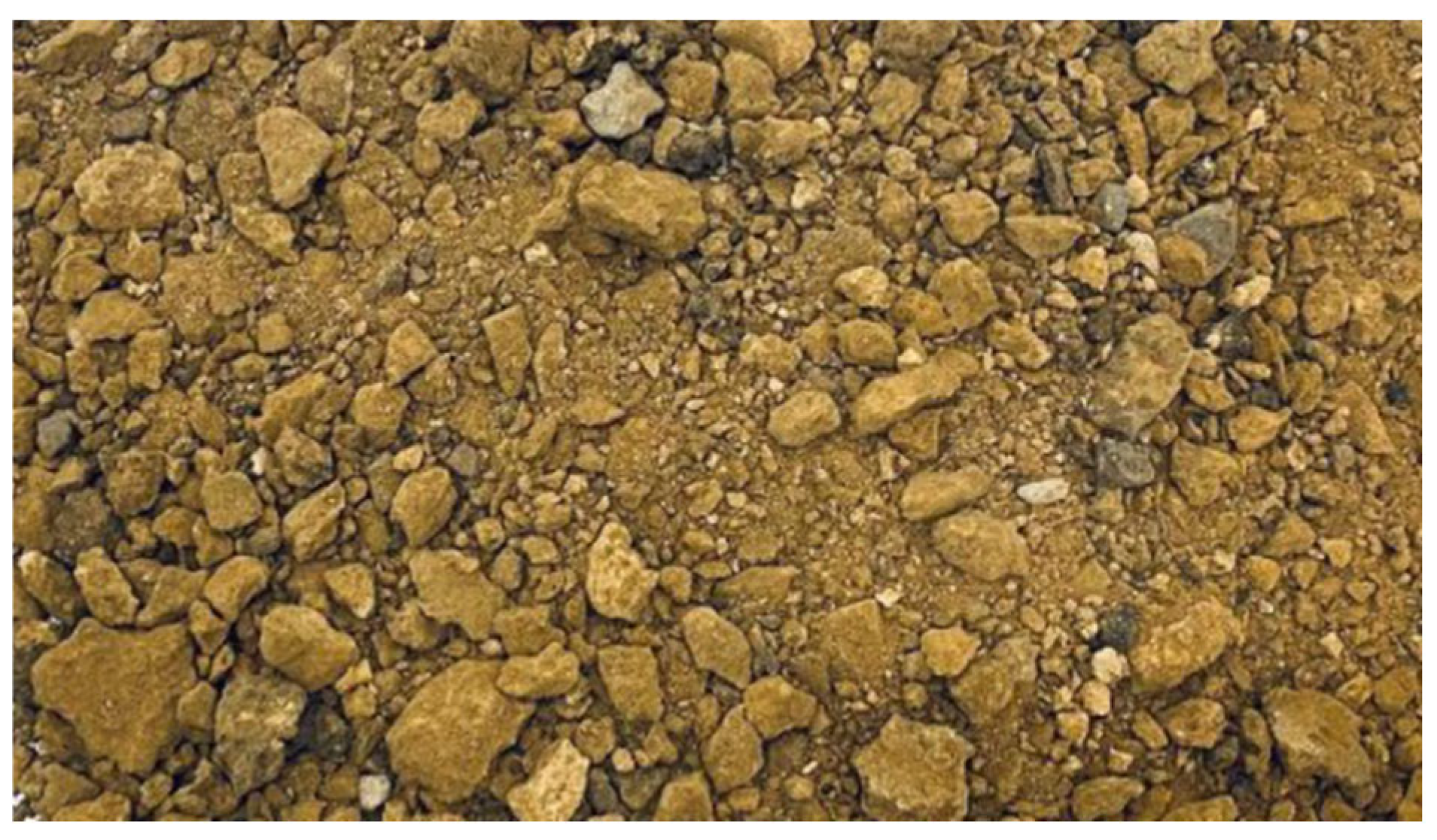
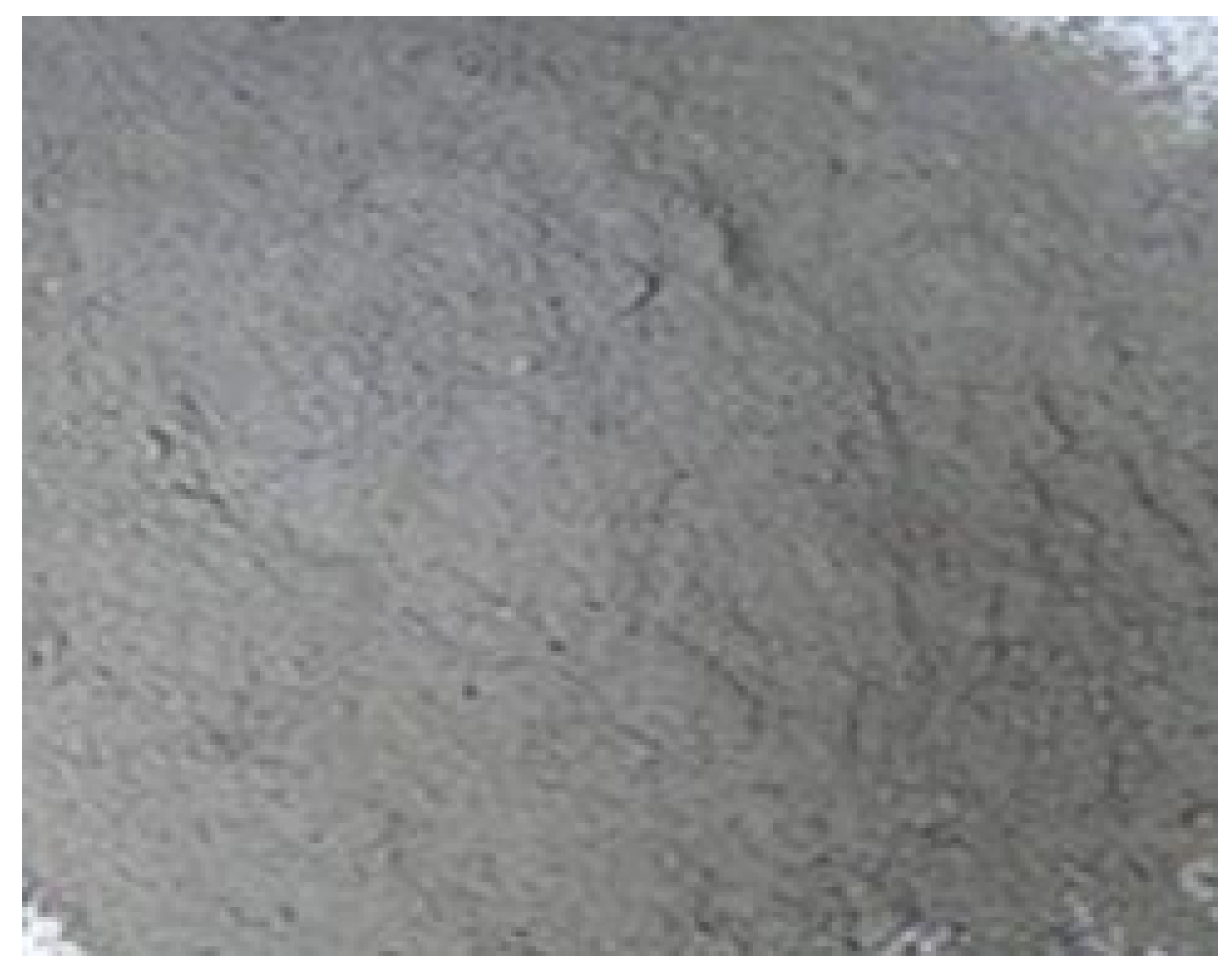
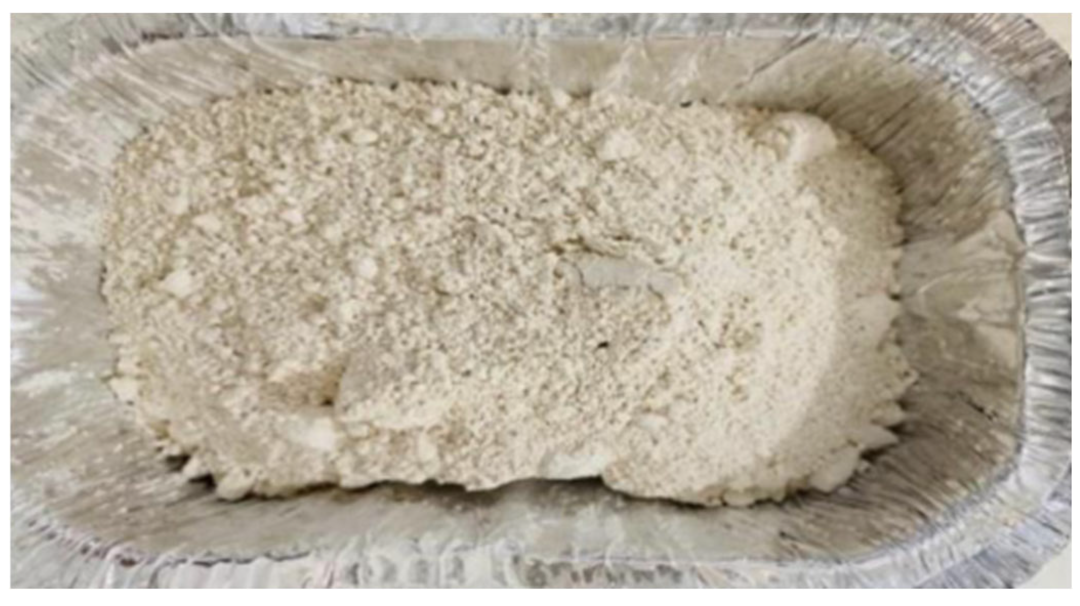
A site visit to the Wurdee Boluc water treatment plant, managed by Barwon Water, was conducted to collect sludge samples (Refer to Figure 2). According to Nguyen et al. [25] the sludge from this site is primarily composed of Poly-Aluminium Chloride (PACl). Samples were characterised as having medium dry strength and low plasticity, with a sandy composition. The plant’s operational practices highlighted the potential for utilising this waste material in construction applications. Table 1 presents the chemical composition of the sludge. Figure 3, Figure 4, Figure 5 and Figure 6 show various materials used in this study.
Due to its widespread availability and versatility, Ordinary Portland Cement (OPC) is the most commonly used binder in various applications. The physical properties of Portland cement used in this project are presented in Table 2.
Lime used in the study was hydrated lime, which was readily available within the geotechnical lab at Deakin University’s Waurn Ponds Campus. The basic constituents of the lime used in the study are listed in Table 3 below.
Different mix designs are developed to evaluate the mechanical performance of sludge combined with soil, lime, and cement. Table 4 shows the details of the mix composition of various samples/tests, all by dry weight. The mix proportions were inspired by previous research by Malkanthi et al. [32] demonstrating optimal strength with a 5% lime and 5% cement combination. These mixtures formed the basis for systematic testing and allowed for the comparison of strength improvements and the relative performance of different compositions.

2.2. Laboratory Testing

2.2.1. Sieve Analysis and Atterberg Limits Test

Sieve Analysis method (AS 1289.3.6.1-2009 [36]) was used to determine the particle size distribution for coarse fraction (>0.075 mm) of soil and sludge. Samples were first washed on 75-micron sieve and then, sieving of samples was done on 300 mm diameter sieves, followed by 200 mm diameter sieves. Hydrometer test is required if more than 10% of material passes through 75 μm sieve. Hydrometer test was done on soil because the results of sieve analysis showed incomplete information and fine fraction (<0.075) for clay was 33%.
Liquid limit, plastic limit and linear shrinkage for soil were examined based on AS 1289.3.1.2-2009 [37], AS 1289.3.2.1-2009 [38] and AS 1289.3.4.1-2008 [39], respectively. These tests were performed on the sample that passed through 425 μm sieve. Liquid limit and plastic limit were then used to estimate the plasticity index of soil.

2.2.2. Compaction Test

Standard Compaction tests were conducted on all samples. These tests were conducted in accordance with AS 1289.5.1.1-2003 [40]. In each test, a sample was compacted in 3 layers in standard compaction mould. Each layer was compacted using 25 hammer blows as listed in AS 1289.5.1.1-2003 [40]. Compaction test helped to determine optimum moisture content and corresponding dry density values for different mixtures. These values of moisture content and dry density were employed in CBR tests.

2.2.3. California Bearing Ratio (CBR) Test

In this study, California Bearing Ratio (CBR) tests were conducted to evaluate the load-bearing capacity of the water treatment sludge mixtures, a critical factor in determining their suitability for road pavement construction. A total of 36 CBR tests were carried out, with three tests conducted for each of the 12 distinct mix compositions. The moisture content for these tests closely approximated the optimum moisture content (OMC) determined through the compaction tests to ensure representative conditions.
All CBR tests were conducted in the unsoaked state. While appropriate for materials operating away from saturation, soaked CBR is often the critical design parameter in subgrade engineering because it reflects worst-case moisture conditions. A planned extension will implement the standard 4-day soaked CBR procedure using the same compaction energy and curing regime, with additional tracking of moisture susceptibility (for example, suction/PI) to permit direct comparison and model retraining that includes moisture state as an explicit covariate.
To assess the effect of compaction on CBR results, three mixtures were prepared using different compaction efforts with 43, 49, and 67 blows. The remaining samples were compacted using a standard effort of 25 blows. The purpose of this variation was to analyse how increasing the number of blows affects the soil’s strength and load-bearing capacity, as measured by the CBR test. By comparing the results, the study aims to determine the influence of compaction energy on soil performance.
The CBR tests included the determination of pressure required for penetration, specifically performing unsoaked CBR tests to assess the soil sample’s resistance to penetration with a standard-sized plunger. Moisture content was determined through the extraction of soil samples from different depths within the CBR tests.
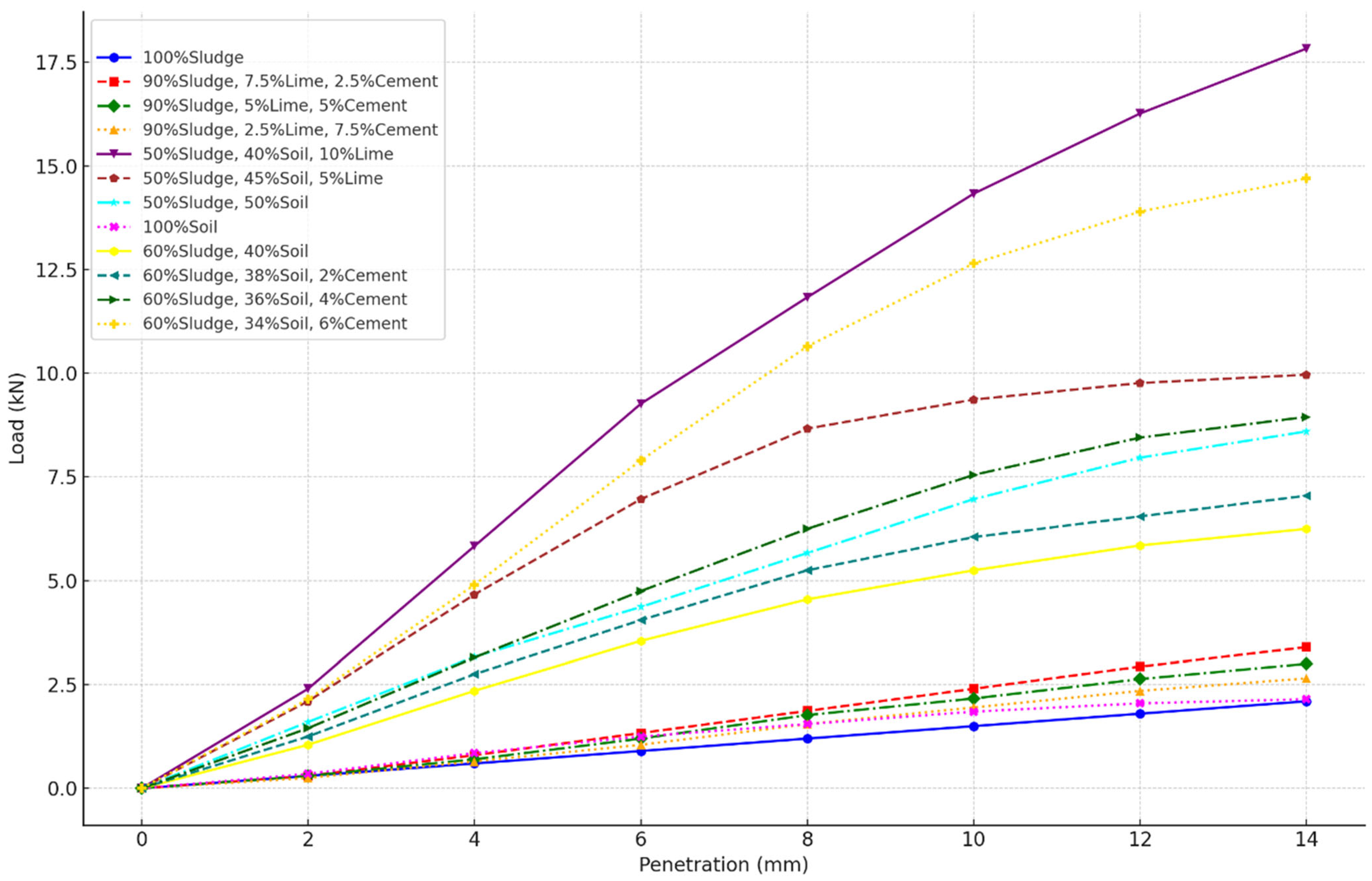
CBR calculations involved plotting load-penetration curves to visualise the relationship between applied force and penetration depth. Force values at penetrations of 2.5 mm and 5.0 mm were read from the curves and bearing ratios for each value were calculated by dividing by the standard loads of 13.2 kN and 19.8 kN, respectively, and then multiplying by 100. The CBR value for each test was reported based on the greater of the two calculated values.

2.3. Data-Driven Modelling

2.3.1. Multiple Linear Regression (MLR)

Multiple Linear Regression (MLR) is a statistical method used to model the relationship between a dependent variable (response variable) and multiple independent variables (predictors). This technique extends simple linear regression by allowing for the inclusion of multiple predictors, enabling researchers and practitioners to capture more complex relationships in the data. MLR assumes that the relationship between the dependent variable and the predictors is linear, and it aims to minimise the error in predicting the dependent variable.
Y = β 0 + β 1 X 1 + β 2 X 2 + + β k X k + ϵ ,
where
  • Y: Dependent variable (outcome to be predicted)
  • β0: Intercept of the regression line (value of Y when all predictors are 0)
  • β1, β2, …, βk: Coefficients of the independent variables X1, X2, …, Xk, representing the change in Y for a one-unit change in the corresponding X, holding other variables constant
  • X1, X2, …, Xk: Independent variables (predictors)
  • ϵ: Error term, accounting for the variability in Y not explained by the predictors

2.3.2. Genetic Programming (GP)

Genetic Programming (GP) is an evolutionary algorithm that generates solutions to problems by evolving symbolic representations, typically in the form of tree structures. These trees represent mathematical expressions, where internal nodes correspond to operations (for example, addition, multiplication), and leaf nodes correspond to variables or constants. GP begins with a randomly generated population of candidate solutions and uses a fitness function to evaluate their performance in solving the given problem. The fitness function is typically defined based on prediction accuracy, such as minimising error metrics like root mean square error (RMSE) or mean absolute error (MAE).
A typical GP model evolves mathematical expressions of the form [41]:
Y = f ( X 1 ,   X 2 ,   ,   X k ) ,
where
  • Y: Output variable or dependent variable.
  • f: Evolved mathematical function or program.
  • X1, X2, …, Xk: Input variables or independent variables.
The fitness function (f) is used to evaluate the quality of a solution:

2.3.3. Dingo Optimisation Algorithm (DOA)

The Dingo Optimisation Algorithm (DOA) is a nature-inspired metaheuristic that mimics the social and foraging behaviours of dingoes. The algorithm initialises a population of virtual dingoes with random positions in the search space. Each dingo represents a potential solution, and its fitness is evaluated based on the objective function [42].
A key feature of DOA is its adaptability, as it dynamically adjusts the balance between exploration and exploitation based on the population’s performance. This flexibility makes it particularly well-suited for optimising GP’s initial population [43]. Additionally, DOA features parameter simplicity, requiring fewer parameters than many other swarm intelligence algorithms, which simplifies its implementation and reduces the need for extensive fine-tuning.
DOA models dingo behaviours through exploration and exploitation phases. Each dingo’s position, xi is updated based on its interaction with pack leaders and other members:
X i t + 1 = X i t + r 1 · L t X i t + r 2 · ( G t X i t ) ,
where
  • X i t + 1 is the position of the i-th dingo at iteration t,
    L t is the position of the local pack leader,
  • G t is the global best solution,
  • r 1 , r 2 are random numbers in [0, 1].

2.3.4. Osprey Optimisation Algorithm (OOA)

The Osprey Optimisation Algorithm (OOA) draws inspiration from the precise hunting strategies of ospreys, focusing on adaptability and efficiency in locating optimal solutions. OOA begins with a population of virtual ospreys, each representing a candidate solution in the search space [44].
In the context of GP, OOA is applied to refine the evolutionary process by dynamically optimising key parameters such as selection and crossover probabilities [45].
OOA updates positions based on a precision-diving mechanism. The position xi of an osprey is refined as [46]:
X i t + 1 = X i t + α   ·   G t X i t + β   ·   ( B i t X i t ) ,
where
  • G t is the global best position,
  • B i t is the best position of the i-th osprey,
  • α and β are learning rates.
maintain balance, OOA adjusts its parameters dynamically:
α = I t e r a t i o n c u r r e n t I t e r a t i o n m a x ,
This ensures the algorithm transitions smoothly from exploration to exploitation.

2.3.5. Rime-Ice Optimisation Algorithm (RIME)

The Rime-Ice Optimisation Algorithm (RIME) models the natural process of rime ice formation, where ice gradually accumulates on surfaces under specific atmospheric conditions. This incremental and controlled buildup is mirrored in RIME’s approach to optimisation, which emphasises gradual refinement of solutions through minor perturbations [46].
In GP, RIME is used to optimise mutation rates, which play a critical role in maintaining population diversity. By introducing controlled variability, RIME ensures that GP avoids premature convergence and explores a broader range of potential solutions. This approach is particularly valuable in later stages of GP, where populations often risk stagnation.
RIME simulates the incremental buildup of ice, gradually refining solutions [47]. Each solution xi is updated as:
X i t + 1 = X i t + γ   ·   G t X i t + δ   ·   ϵ ,
where
  • γ controls the exploitation rate,
  • Gt is the global best solution,
  • δ⋅⋅⋅ϵ introduces controlled random perturbations.
Similarly to simulated annealing, RIME incorporates a cooling schedule to reduce perturbation over time:
δ = δ 0   ·   e x p ( t T ) ,
where δ 0 is the initial perturbation rate, t is the current iteration, and T is the total number of iterations.

2.3.6. Co-Evolutionary Framework

The co-evolutionary framework combines the strengths of GP and nature-inspired optimisation algorithms like DOA, OOA, and RIME to create a synergistic system [48,49]. The core concept of this framework lies in the synergy between GP and nature-inspired optimisation algorithms. GP evolves symbolic structures by generating models or equations that describe the relationships between variables, often represented as tree structures, which are refined through genetic operators such as crossover, mutation, and reproduction. Meanwhile, nature-inspired algorithms refine parameters by optimising the numerical components, such as coefficients, thresholds, or weights, within the symbolic models to maximise their performance on the objective function, such as minimising error or enhancing efficiency. This dual approach ensures that the models are not only interpretable and mathematically robust but also fine-tuned for optimal numerical accuracy and real-world applicability [50,51,52]. In this study, the following steps were undertaken to implement the Co-Evolutionary Framework:
  • Step 1: Initialisation
GP initialises a population of symbolic models, each representing a potential solution to the problem.
Nature-inspired algorithms (e.g., DOA, OOA, RIME) initialise populations of candidate parameter sets for the symbolic models.
  • Step 2: Fitness Evaluation
GP evaluates the fitness of symbolic models based on a predefined criterion, such as the Mean Squared Error (MSE) between predicted and actual values.
The optimisation algorithm evaluates parameter sets by substituting them into the symbolic models and calculating fitness scores.
  • Step 3: Co-Evolutionary Loop
GP performs genetic operations (crossover, mutation, and reproduction) to evolve better symbolic models.
These operations allow GP to explore the space of possible model structures, focusing on those that better fit the data.
The optimisation algorithm (e.g., DOA, OOA, RIME) refines the parameters of the symbolic models evolved by GP.
The optimised parameters are fed back to GP, improving the evaluation of symbolic models.
This feedback ensures that GP evolves models that are not only structurally sound but also numerically precise.
  • Step 4: Termination
The process continues until a stopping criterion is met, such as a maximum number of generations, a threshold error, or a lack of improvement in fitness.
The Co-Evolutionary Framework provides symbolic interpretability, as GP generates human-readable models that offer clear insights for decision-makers. The framework also ensures numerical precision, with nature-inspired algorithms fine-tuning the parameters of these models for high accuracy. Through dynamic adaptation, the co-evolutionary loop continuously refines both the symbolic and numerical aspects of the models, ensuring robustness and flexibility in addressing varying problem complexities. Additionally, the framework achieves improved search efficiency, as nature-inspired algorithms guide parameter optimisation, effectively reducing the search space for symbolic evolution and accelerating convergence toward optimal solutions.

2.4. Uncertainty Quantification

To communicate the reliability of point predictions, 95% prediction intervals (PIs) are reported for all models. PIs are constructed to bound the likely observed CBR at a given input.
For each model, residuals r i = y i y ^ i are sampled with replacement and added to the fixed predictions y ^ i to form bootstrap replicates of the observation, y ~ b , i = y ^ i + r i \ * ( b ) (pairs of residuals per bootstrap draw). Across B = 2000 replicates, the 2.5th and 97.5th percentiles at each observation yield 95% PIs. This approach is model-agnostic, provides calibration against moderate misspecification, and permits consistent comparison across linear (MLR) and nonlinear (GP) predictors.
Two diagnostics are reported for each model: (i) empirical coverage (percentage of observations contained within the 95% PI) and (ii) median PI width (CBR%), which reflects precision at comparable coverage. Parity plots overlay point predictions with 95% PIs; complementary “width vs. prediction” plots illustrate how uncertainty varies across the response range.

2.5. Small-Sample Validation and Overfitting Control

To reduce overfitting risk under a small dataset, model selection and performance estimation were conducted using nested cross-validation (CV) combined with a label-permutation (y-randomisation) test.
An outer 5-fold CV estimated generalisation performance, while an inner 3-fold CV tuned hyperparameters. Preprocessing included median imputation and standardisation for numeric predictors, and imputation plus one-hot encoding for categorical predictors. Two model families were evaluated: Ridge regression (α ∈ {0.01, 0.1, 1, 10, 100}) and Gradient Boosting Regressor (n_estimators ∈ {50, 100}; max_depth ∈ {2, 3}; learning_rate ∈ {0.05, 0.1}; subsample ∈ {0.8, 1.0}). Performance metrics on the held-out outer folds were R2, MAE, and RMSE.
To verify that the observed performance was not driven by chance correlations, we ran a 200-run label-permutation test. The model class and hyperparameters were fixed to those selected on the non-permuted data, and the original 5-fold splits were reused at every run. For each permutation, we randomly shuffled the target vector, retrained on the training folds, and recorded the mean CV R2 on the held-out folds to form a null distribution.

3. Geotechnical Results

3.1. Sieve Analysis and Atterberg Limits Test Results

Figure 7 illustrates two particle size distribution curve tests for soil and alum sludge. The curves show the percentage of finer particles as a function of particle size on a logarithmic scale. The results indicate that the particle size distributions are consistent within each material type. Both tests 1 and 2 for soil exhibit similar particle size curves and indicate comparable textures, and tests 1 and 2 for Alum sludge also display nearly identical curves and reflect a consistent proportion of fine particles.

3.2. Compaction Test Results

Achieving optimal compaction is crucial in geotechnical and environmental engineering, as it directly influences the strength and stability of treated soil materials. In this study, a total of 12 tests were conducted on 12 different mixtures, including at least 4 compaction tests for each mixture, to evaluate the influence of sludge, soil, cement, and lime on compaction behaviour. Figure 8 presents the relationship between optimum moisture content (OMC) and maximum dry density (MDD) for various material compositions and highlights the influence of sludge, soil, cement, and lime on compaction behaviour. Mixtures with higher soil content, such as 50% Soil and 50% Sludge, achieve a relatively high MDD with lower OMC and indicate effective compaction with less moisture. In contrast, mixtures with higher sludge content exhibit increased OMC and reduced MDD, such as 100% Sludge. Mixtures with balanced proportions, such as 50% soil and 50% sludge, display a well-defined peak dry density at their OMC and indicate efficient compaction. Meanwhile, sludge-dominant mixtures show flatter curves and lower peak densities and signify reduced compaction efficiency. The addition of cement or lime to sludge mixtures significantly improves peak dry density and narrows the moisture range for effective compaction. These results emphasise the potential for optimised sludge-soil mixtures to balance environmental sustainability and engineering performance, particularly when combined with minimal amounts of stabilisers.

3.3. California Bearing Ratio (CBR) Test Results

Figure 9 illustrates the load-penetration behaviour of various material compositions, further reinforcing the potential of sludge as an eco-friendly stabiliser. Mixtures with balanced sludge content, such as 50% Sludge and 50% Soil, exhibit a load-bearing capacity that is competitive with cement and lime-stabilised combinations. While higher sludge proportions, such as 100% Sludge, result in reduced load capacity, moderate sludge usage optimises both performance and sustainability. By recommending sludge over cement and lime, this approach aligns with environmental goals and offers a viable solution to reduce carbon emissions and promote the reuse of industrial byproducts.
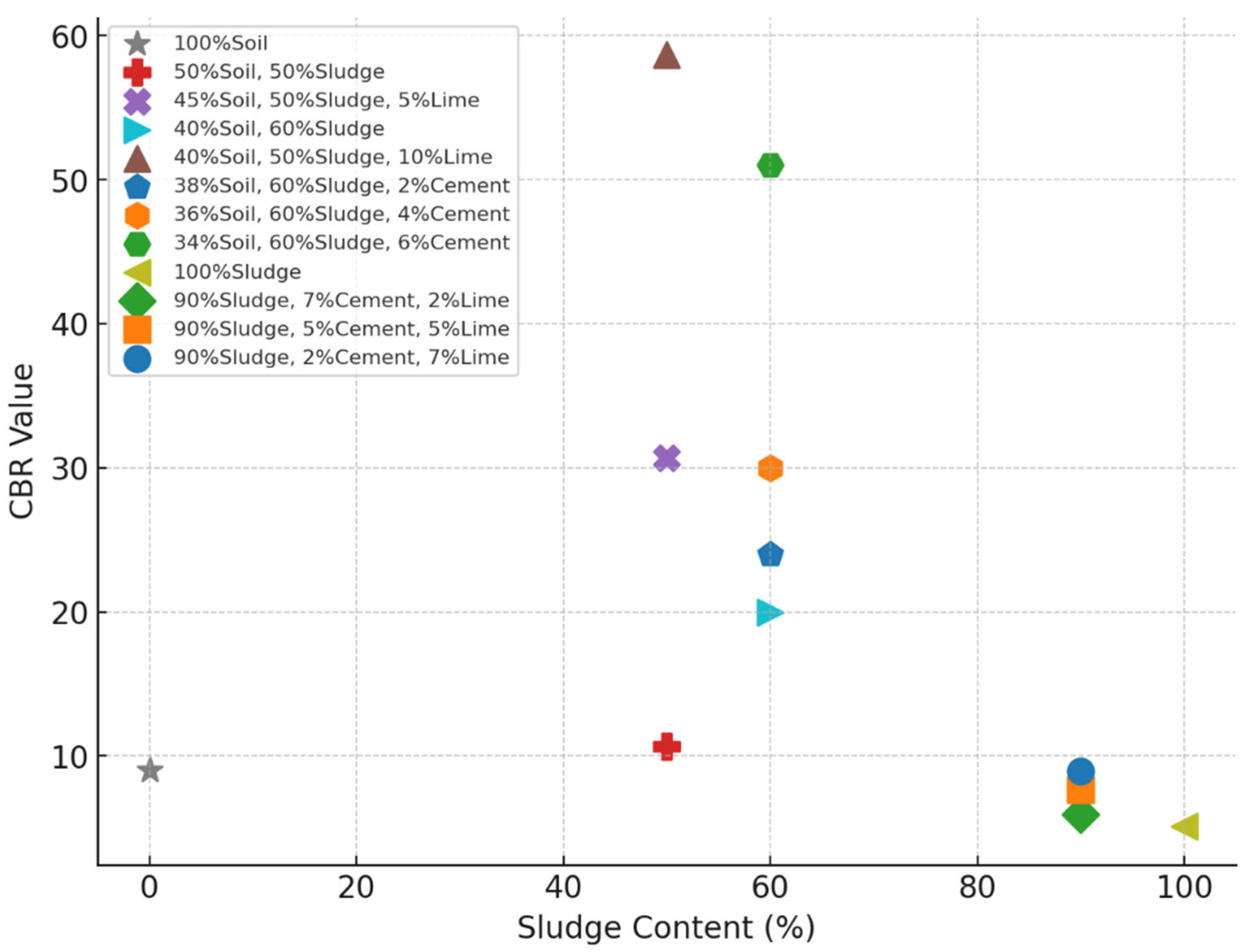
Figure 10 demonstrates the relationship between sludge content and CBR values and emphasises the potential for optimising sludge usage in soil stabilisation. While pure sludge exhibits relatively low CBR values, a balanced combination of sludge and soil, such as 50% sludge and 50% soil, demonstrates a significant improvement in CBR. This suggests that incorporating sludge in moderate proportions can enhance the mechanical properties of the mixture. Cement and lime-stabilised mixtures, such as 50% sludge, 40% soil, and 10% lime, achieve the highest CBR value. The results indicate that with an optimal sludge percentage, comparable performance can be achieved while promoting sustainable practices.

3.4. Evaluating the Effect of Input Parameters

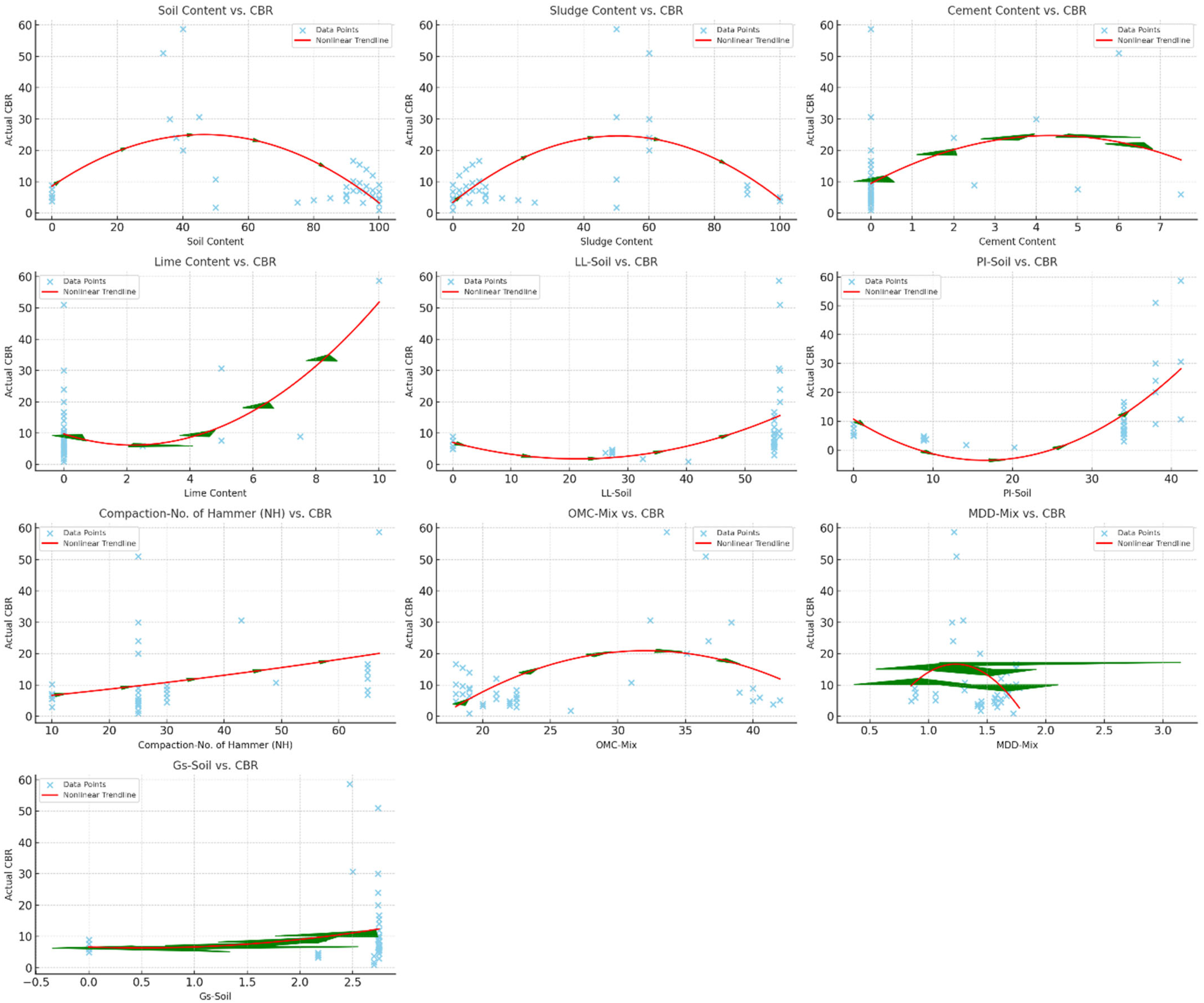
Figure 11 provides a detailed analysis of the relationships between various parameters and the CBR. The red curves represent quadratic trendlines that capture nonlinear variations, while the green arrows emphasise the direction of the trends. Each plot highlights the impact of individual parameters, such as soil content, sludge content, cement content, and others, on the soil’s strength as measured by CBR.
For soil content and sludge content, the trendlines show parabolic behaviour, where the CBR increases to an optimal point and then decreases. These trendlines suggest that while higher soil or sludge content may improve cohesion or compaction to a certain extent, excessive amounts could weaken the soil structure. This could be due to an imbalance between fine and coarse particles that can lead to reduced load-bearing capacity. Sludge, being organic, may also degrade under high proportions, adversely impacting the soil’s performance.
Lime content represents a strong positive correlation with CBR, particularly at higher levels, as indicated by the upward curve. Lime acts as a stabiliser and improves soil strength by reducing plasticity and increasing pozzolanic reactions. These chemical reactions lead to the formation of cementitious compounds, which enhance the load-bearing capacity of the soil. This trend is consistent with established geotechnical practices, where lime is widely used to improve the performance of fine-grained soils.
Other parameters, such as plasticity index (PI-Soil), compaction (no. of hammer blows), and optimum moisture content (OMC-Mix), also show distinct trends. For example, increasing the number of hammer blows improves compaction and results in higher CBR values due to better particle interlocking. However, the influence of OMC-Mix appears nonlinear, likely due to the need for an optimal moisture level for effective compaction. Excessive moisture can reduce strength, while insufficient moisture leads to incomplete compaction. These trends highlight the importance of achieving a balanced mix of soil properties to optimise load-bearing capacity in geotechnical applications.
In Figure 11, the trendlines in these graphs are generated using nonlinear regression techniques to fit a curve that best represents the relationship between CBR and various influencing factors such as soil, sludge, cement, lime content, and compaction parameters.
The 3D surface plot in Figure 12 also illustrates the relationship between optimum moisture content (OMC-Mix), maximum dry density (MDD-Mix), and the California bearing ratio (CBR). The surface, smoothed using cubic interpolation, reveals a continuous gradient of CBR values. This figure illustrates that as OMC-Mix and MDD-Mix increase, the CBR value also increases, reaching a peak. However, beyond this peak, further increases in OMC-Mix and MDD-Mix lead to a decrease in CBR values.
Figure 11 and Figure 12 show that different parameters have different effects on CBR values. Therefore, new approaches like machine learning methods and algorithms need to be developed.
The CBR values of the untreated natural soil were relatively low (~5–8%), which is typical for fine-grained subgrade materials with limited load-bearing capacity. With the incorporation of WTS alone, the CBR initially decreased due to the high fines and organic content of the sludge, which increased plasticity and weakened the soil matrix. However, when the sludge was combined with a small amount of lime or cement, the CBR values increased substantially because pozzolanic reactions and cation exchange improved particle bonding and reduced plasticity.
The mixtures containing 10% lime consistently showed the highest strength gains. The optimum blend (40% soil + 50% WTS + 10% lime) achieved a peak CBR of 58.7%, which represents an increase in more than ~550% relative to the untreated soil. This improvement clearly indicates a significant enhancement in shear strength and stiffness of the subgrade material.

4. Database Preparation

After collecting all results from the laboratory, they were combined with results in published literature. The published database includes results from Shah et al. [53], Baghbani et al. [27], and Jadhav et al. [54]. The final database comprises 40 observations for each parameter and highlights a diverse range of material properties relevant to soil and sludge mixtures. Table 5 presents statistical information from such a database. The CBR values range from 0.9 to 58.67, with a mean of 11.29 and a standard deviation of 12.26 that reflects significant variability in load-bearing capacity. Soil content and sludge content exhibit wide ranges (0 to 100%) with mean values of 69.2% and 29.38%, respectively, that indicate their predominant contributions to the mixtures. Cement and lime content are relatively lower, with mean values of 0.68% and 0.75%, and maximum values of 7.5% and 10.0%, respectively, for cement and lime. Liquid limit (LL-Soil) and plasticity index (PI-Soil) have averages of 42.50 and 25.55, which show moderate plasticity in the mixtures. Compaction-related parameters, such as the number of hammer blows (NH), have a mean of 31.6, and the optimum moisture content (OMC) averages 25.99%, which suggests consistent compaction requirements. Maximum dry density (MDD-Mix) averages 1.443 g/cm3, with a range of 0.854 to 1.775, while specific gravity (Gs-Soil) varies up to 2.75 with a mean of 2.36, reflecting typical values for mineral-based materials. This variability shows the heterogeneity of the dataset and its potential applications in soil stabilisation and pavement engineering.
Figure 13 presents box plots illustrating the distribution of various geotechnical parameters, including soil content, sludge content, compaction characteristics, and CBR values. The spread and interquartile ranges highlight variability in these properties, with soil and sludge content exhibiting wider distributions, while parameters like specific gravity (Gs-Soil) and MDD-Mix show more consistent values with minimal variation.
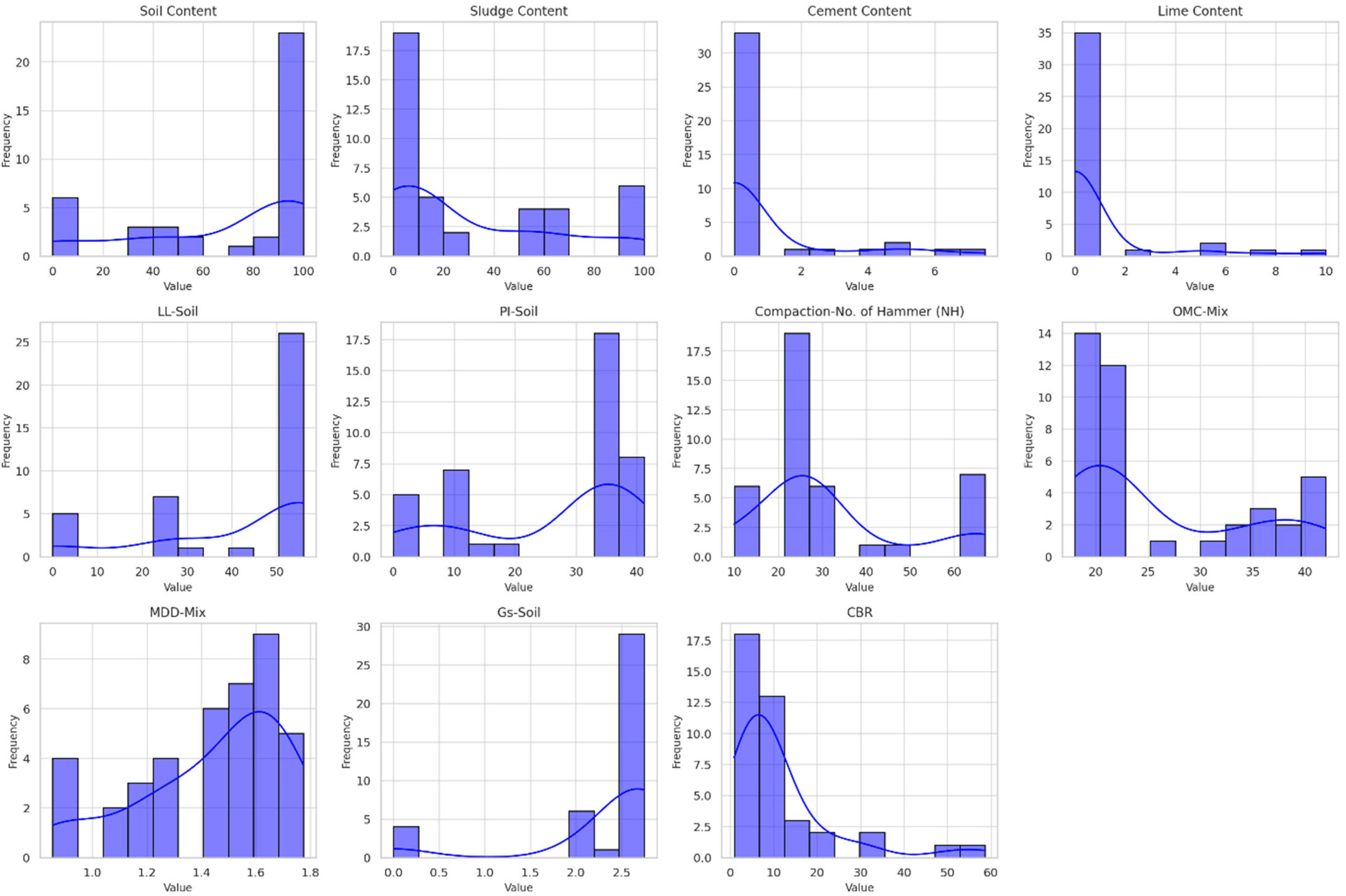
Figure 14 presents histograms for key parameters related to soil and sludge mixture properties, illustrating their frequency distributions across the dataset. Variables are soil content, sludge content, cement content, lime content, liquid limit (LL-Soil), plasticity index (PI-Soil), compaction (number of hammer blows), optimum moisture content (OMC-Mix), maximum dry density (MDD-Mix), specific gravity (Gs-Soil), and California bearing ratio (CBR). The histograms represent the variability and central tendencies of each parameter, with notable trends such as the clustering of soil content and sludge content values around higher percentages, while cement and lime contents are predominantly low. Parameters like CBR and MDD-Mix show a broader range of values and indicate diverse material behaviours, which are critical for understanding the mixture’s suitability for construction applications.
A 75–25% train-test split was chosen to ensure a sufficient number of samples for model training while retaining enough data for reliable performance evaluation. This ratio is commonly used in machine learning studies to balance model learning and generalisation, especially in small to medium-sized datasets. Table 6 and Table 7 show the statistical information of these two databases. Based on the statistical information provided, the two databases have good statistical similarity, which shows that 30 data sets were used for training and 10 for testing. The small number of data sets for training and testing is one of the points that should be considered in future research, but at this stage, this number of data sets was the largest database currently available in the history of studies.
Minimum, maximum, and mean values of CBR for the training database are 0.9, 58.7, and 10.6 (Table 6), and for the testing database are 3.8, 51.0, and 13.3 (Table 7). It is considered that the range provided for all parameters for the training database is larger than the range for the testing database. This will provide greater accuracy in the results obtained from the testing database.
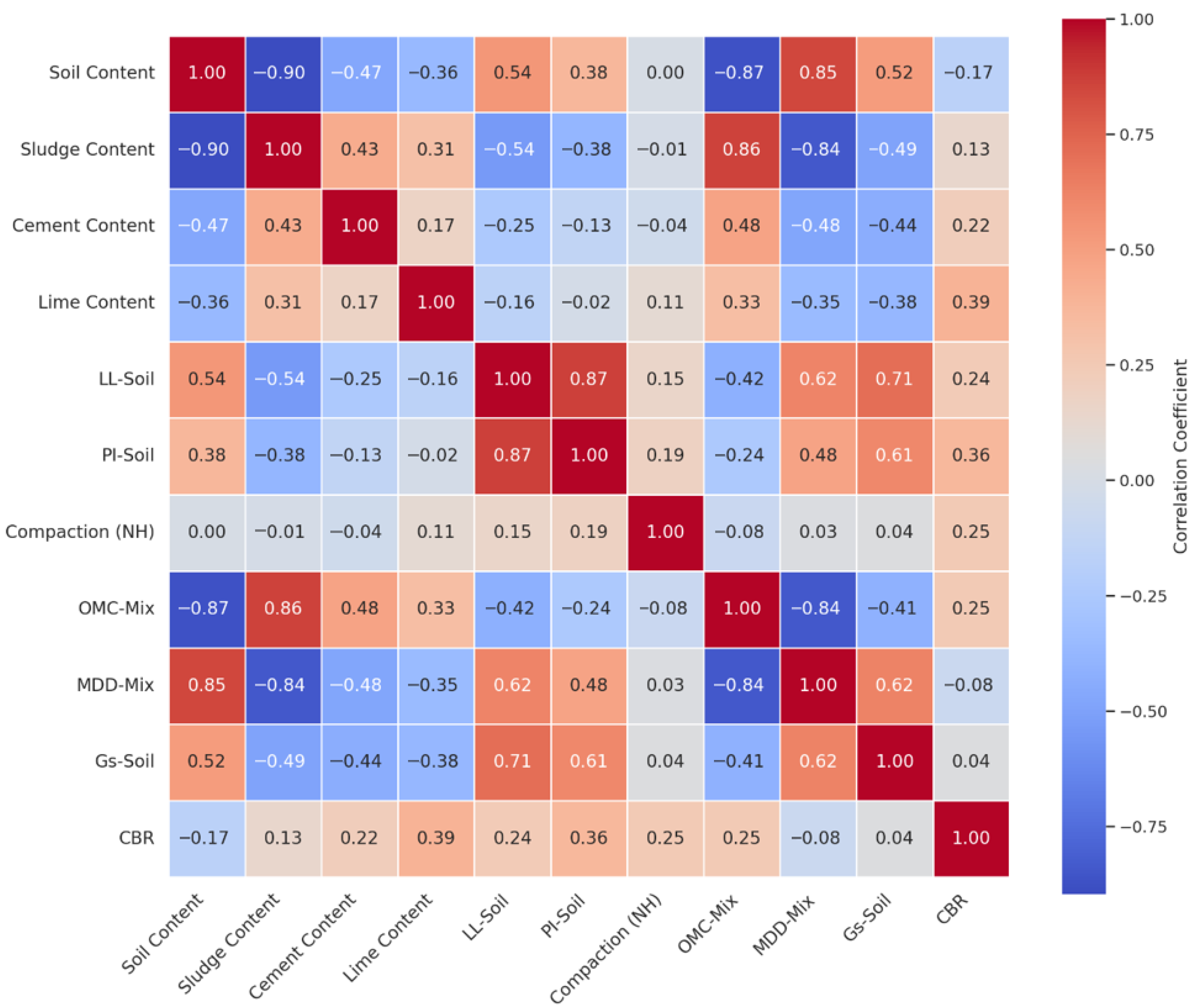
The heatmap in Figure 15 visually represents the relationships between key variables in the dataset. Correlation analysis plays a crucial role in understanding the interdependencies between various geotechnical parameters, influencing both the interpretation of results and the formulation of engineering recommendations. Strong positive correlations, such as between LL-Soil and PI-Soil (0.87), confirm expected relationships where higher liquid limit soils tend to have a higher plasticity index and affect soil workability and strength. Similarly, the strong correlation between MDD-Mix and Soil Content (0.85) reinforces the idea that higher soil content contributes to greater compaction efficiency, which is essential for foundation stability.
On the other hand, strong negative correlations, such as between Soil Content and Sludge Content (−0.90) and OMC-Mix and MDD-Mix (−0.84), indicate inverse relationships that must be considered in material selection and stabilisation strategies. The inverse correlation between OMC and MDD suggests that materials requiring higher moisture content for compaction tend to achieve lower dry densities, which can affect pavement performance and bearing capacity. Additionally, the weak correlation between CBR and Soil Content (−0.17) and CBR and Sludge Content (0.13) suggests that CBR performance is influenced by other factors such as cement and lime stabilisation, rather than soil-sludge ratios alone. These findings highlight the importance of using a combination of material compositions and stabilisation techniques rather than relying solely on individual parameters for strength improvements.
Since the linear correlation values between most parameters are below 0.8–0.9, the parameters do not exhibit a strong relationship and can be treated as independent variables in regression and machine learning models. Additionally, as the correlation between CBR and other parameters remains below this threshold, more advanced models, such as machine learning techniques, are required instead of simple linear regression to accurately predict CBR values.
The database was normalised linearly using Equation (8):
X n o r m = X X m i n X m a x X m i n ,
where
  • Xnorm is the normalised value,
  • X is the original value,
  • Xmin is the minimum value in the dataset,
  • Xmax is the maximum value in the dataset.
This normalisation ensures that all values fall within a standard range, between 0 and 1, making data comparable and improving the performance of machine learning models by preventing large values from dominating. It also eliminates unit dependency, enhances numerical stability in calculations, speeds up model convergence, and makes data visualisation more intuitive by revealing clearer patterns and trends.

4.1. Nested Cross-Validation Results

Across outer folds, the Gradient Boosting pipeline delivered consistent generalisation, achieving R2 = 0.867 ± 0.049, MAE = 2.329, and RMSE = 3.863 (mean ± SD over five folds). In contrast, Ridge regression exhibited substantial fold-to-fold variability with R2 = 0.319 ± 1.441, MAE = 1.599, and RMSE = 2.402, including a negative-R2 fold indicative of a mismatch to underlying nonlinearity in the CBR response.
Hyperparameter choices were comparatively stable for Gradient Boosting: n_estimators = 100 (5/5 folds), subsample = 0.8 (4/5), learning_rate = 0.1 (3/5) or 0.05 (2/5), and max_depth = 2 (3/5) or 3 (2/5). For Ridge, the most frequent setting was α = 1.0 (3/5 folds), with occasional α = 0.1 and α = 10.0 on individual folds. This pattern supports the preference for a shallow, regularised ensemble that captures nonlinear structure while maintaining stable complexity across resamples (refer to Table 8).

4.2. Permutation Test for Model Validity

A label-permutation (y-randomisation) procedure was conducted to verify that the predictive performance was not an artefact of chance correlations. Using 200 permutations and 5-fold cross-validation, the best-performing pipeline, Gradient Boosting with hyperparameters fixed from the nested-CV selection, was re-evaluated by shuffling the target labels while keeping the full preprocessing and model structure unchanged. The resulting null distribution reflects the level of performance expected if no real relationship existed between predictors and Actual CBR.
The observed mean CV performance for the unshuffled data was R2 = 0.883, while the empirical probability of attaining an equal or greater score under the null was p ≈ 0.005. The null distribution of mean CV R2 lay well below the observed value, indicating strong separation and providing evidence that the model captures a genuine signal rather than overfitting noise (refer to Figure 16).

5. CBR Prediction Results

5.1. Multiple Linear Regression (MLR) Results

Linear regression of measured and predicted CBR values is plotted for all database as shown in Figure A1a. It shows that the prediction accuracy of the MLR model is suboptimal and suggests the need for more advanced machine learning methods and algorithms. The line chart highlights significant deviations between the measured and predicted CBR values, especially for higher CBR values, and indicates that the MLR model struggles to accurately capture the complex relationships in the database. Furthermore, the histogram of absolute residual errors shows a widespread distribution, with residuals exceeding 10 for multiple cases and even reaching values above 25 (Figure A1b). These larger errors suggest that the linear assumptions of MLR are insufficient for modelling the nonlinear and potentially multi-dimensional nature of the data. To improve prediction performance and reduce residual errors, machine learning algorithms could be employed to better capture the underlying patterns and complexities in the database.
Figure A2 compares the measured and predicted CBR values using the MLR model for both training and testing databases, along with the ideal prediction line (y = 1x), 10% deviation bounds (y = 0.9x and y = 1.1x), and a 95% confidence interval. The plot shows that many points, particularly from the testing database, deviate significantly from the perfect prediction line and indicate poor generalisation of the MLR model to unseen data. While some training points fall within the 10% deviation bounds, the testing points often lie outside these bounds and show that the model struggles to accurately predict CBR values in the higher range. The widening confidence interval at higher values further shows the limitations of the MLR model in capturing the underlying complexity of the data. These results highlight the need for more advanced machine learning algorithms to improve prediction accuracy and reliability.
Equation (9) was derived based on this MLR model to predict CBR.
C B R = 123.5 1.1 × X 1 0.9 × X 2 + 1.4 × X 3 + 0.8 × X 5 0.5 × X 6 + 0.1 × X 7 0.5 × X 8 22.5 × X 9 + 5.2 × X 10 ,
where X1, X2, X3, X4, X5, X6, X7, X8, X9, X10 are soil, sludge, cement, lime content, LL-Soil, PI-Soil Compaction-No. of Hammer (NH), OMC-Mix, MDD-Mix, Gs-Soil, respectively.
Table 9 provides the performance metrics for the MLR model and highlights the disparity in its predictive accuracy between the training and testing datasets. The MAE for the training database is 3.748, which increases significantly to 6.529 for the testing database. These results indicate poorer accuracy on unseen data. Similarly, the MSE jumps from 26.914 in training to 114.083 in testing, and the RMSE more than doubles from 5.188 to 10.681. The coefficient of determination (R2) is 0.753 for training but drops to 0.552 for testing. These metrics collectively demonstrate the MLR model’s limitations and suggest the need for more sophisticated machine learning approaches to enhance predictive performance and generalisation.

5.2. Genetic Programming-Dingo Optimisation Algorithm (GP-DOA)

Figure A3a demonstrates the improved predictive performance of the GP-DOA model as compared to the MLR model (Figure A1a) in estimating CBR values. In Figure A3a, the predicted values from the GP-DOA model align more closely with the measured CBR values and maintain consistency across the entire database. Unlike the MLR model, which showed significant deviations at higher CBR values, the GP-DOA model demonstrates a more accurate fit even for the peak values and indicates its superior ability to handle nonlinearities and complex patterns in the data.
The histogram of absolute residual errors in Figure A3b further highlights the enhanced performance of the GP-DOA model. The residual errors are smaller and more tightly distributed around lower values, with the majority concentrated below 3. This contrasts sharply with the MLR model (Figure A1b), which showed a broader error distribution and higher residuals. The smaller errors in the GP-DOA model indicate higher prediction accuracy and better generalisation capability. Overall, the GP-DOA model effectively addresses the limitations of the MLR model by leveraging advanced optimisation techniques to achieve significantly better results.
Figure A4 illustrates the performance of the GP-DOA model in predicting CBR values for both training and testing databases. The predicted values align closely with the measured values, as evidenced by the concentration of data points along the perfect fit line (y = 1x) and within the 10% deviation bounds (y = 0.9x and y = 1.1x). The 95% confidence interval remains relatively narrow, even at higher CBR values, and indicates consistent and reliable predictions across the dataset. This contrasts with the MLR model (Figure A2), where larger deviations and a broader confidence interval were observed. The GP-DOA model demonstrates superior generalisation, particularly in the testing data, and confirms its ability to capture the complex, nonlinear relationships within the data with high accuracy.
Equation (10) is the outcome of GP-DOA model to predict CBR. In Equation (10), all input parameters are normalised values from 0 to 1 based on Equation (12).
C B R = ( ( ( ( ( X 6 × X 7 × ( X 5 + r 3 ) ) × ( X 2 × X 10 + X 3 2 ) ) × ( X 6 × X 4 X 2 + X 10 + X 5 2 X 2 X 7 ) ) × ( ( ( X 7 X 8 ) 2 + X 6 × X 10 × X 6 2 ) ( ( 2 × X 5 × X 8 ) × ( ( X 1 X 2 ) × ( X 9 + X 1 ) ) ) ) ) + ( X 3 × X 6 × X 3 × X 2 + r 3 r 1 ) ) ,
where X1, X2, X3, X4, X5, X6, X7, X8, X9, X10 are soil, sludge, cement, lime content, LL-Soil, PI-Soil Compaction-No. of Hammer (NH), OMC-Mix, MDD-Mix, Gs-Soil, respectively.
Also, r1, r2, and r3 are constants and equal to 0.847, 0.3576, and 0.9487, respectively.
Table 10 shows the performance metrics of the GP-DOA model and highlights its exceptional predictive accuracy and generalisation capability. The MAE is significantly low, with 2.030 for the training database and an even lower 1.800 for the testing database and indicates consistent precision across both datasets. Similarly, the MSE and RMSE values are small, with 6.370 and 2.524 for training and 4.383 and 2.094 for testing, respectively, further emphasising the model’s ability to minimise prediction errors. The R2 values of 0.941 for training and an impressive 0.983 for testing demonstrate the GP-DOA model’s strong ability to capture the variability in the data and generalise effectively to unseen data. These metrics confirm that the GP-DOA model significantly outperforms traditional MLR and makes it a strong choice for predicting complex relationships in CBR databases.

5.3. Genetic-Osprey Optimisation Algorithm (GP-OOA)

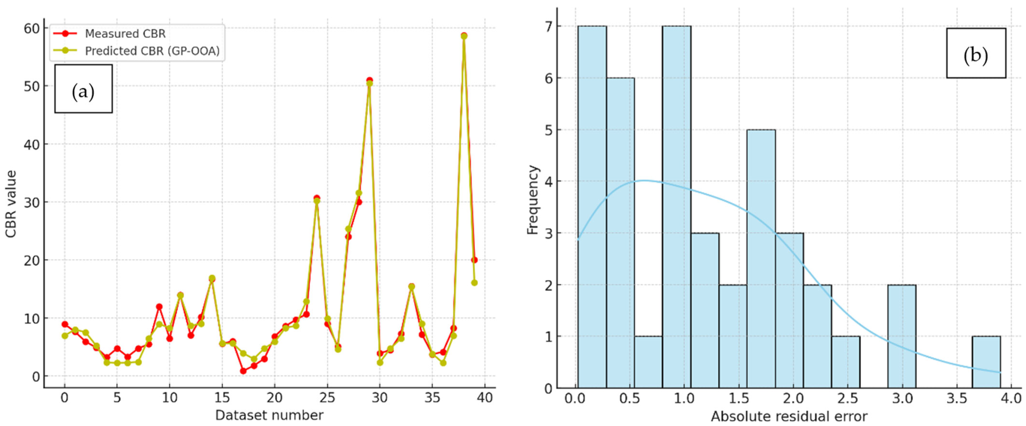
The results presented in Figure A5 demonstrate the superior performance of GP-OOA in predicting CBR values. In Figure A5a, the predicted values align almost perfectly with the measured values across the entire dataset, showcasing the model’s ability to capture both linear and nonlinear patterns effectively. Unlike other models, GP-OOA exhibits minimal deviations, even for the highest CBR values, maintaining consistent accuracy throughout. This high degree of alignment indicates the GP-OOA model’s enhanced ability to generalise complex data relationships, outperforming the GP-DOA model in terms of precision and reliability.
The histogram presented in Figure A5b further supports this conclusion by illustrating the absolute residual errors of the GP-OOA model. The residual errors are tightly concentrated within a range of 0 to 2, with most errors falling below 1, indicating exceptional prediction accuracy. The distribution is much narrower compared to GP-DOA, showing that GP-OOA significantly reduces prediction errors and provides a better fit for both training and testing datasets. The consistently low errors and the close match between measured and predicted values highlight that the GP-OOA model is an advanced and effective tool for predicting CBR, surpassing the performance of the GP-DOA and MLR models.
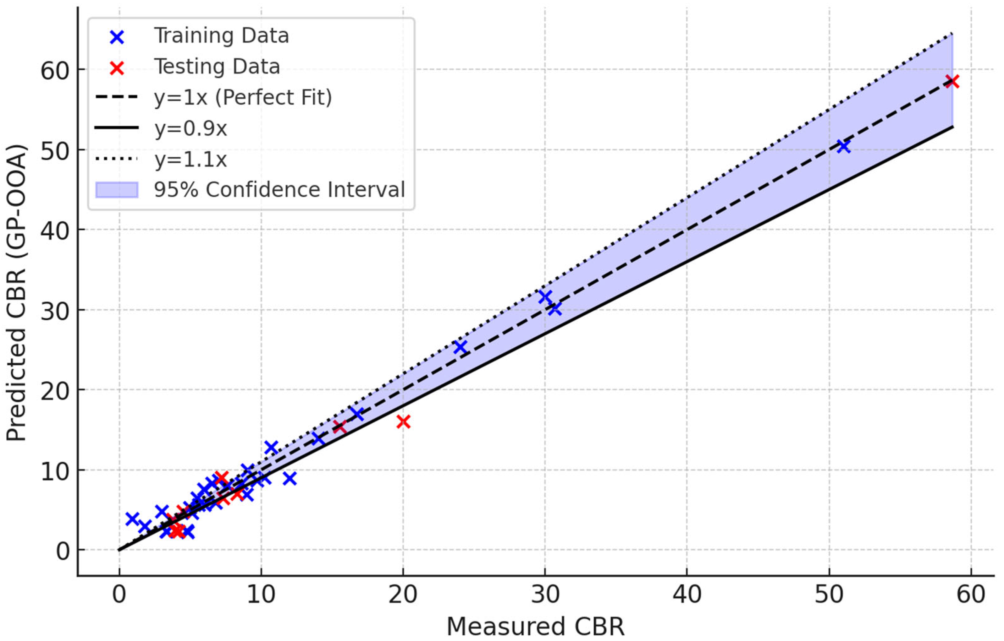
Figure A6 demonstrates the excellent performance of the GP-OOA in predicting CBR values for both training and testing databases. The predicted values align very closely with the measured values along the perfect fit line (y = 1x), with most points falling within the 10% deviation bounds (y = 0.9x and y = 1.1x). The 95% confidence interval remains narrow throughout, even for higher CBR values, and shows the model’s precision and consistency. Compared to previous models like GP-DOA and MLR, the GP-OOA model exhibits significantly reduced variability and enhanced predictive accuracy and indicating its superior capability to capture complex data patterns and generalise effectively across both training and testing datasets.
Following formula is outcome of GP-OOA model to predict CBR. In Equation (11), all input parameters are normalised values from 0 to 1 based on Equation (11).
C B R = ( ( ( r 3 r 3 2 × ( X 7 X 10 ) × X 2 2 × X 3 2 ) ( X 8 X 7 ) 4 × ( X 8 × r 1 × ( X 5 X 7 ) + r 3 2 + X 8 X 7 ) ) × ( ( ( ( r 1 r 2 ) × ( r 1 X 6 ) ) 2 + ( X 6 × ( X 4 × r 1 X 4 + X 6 ) ) ) × ( X 8 × ( X 2 X 1 ) × ( X 6 + X 8 ) + ( r 1 2 × ( X 3 + r 2 ) + ( X 9 + X 7 ) × ( X 3 + X 4 ) ) ) ) ) ,
where X1, X2, X3, X4, X5, X6, X7, X8, X9, X10 are soil, sludge, cement, lime content, LL-Soil, PI-Soil Compaction-No. of Hammer (NH), OMC-Mix, MDD-Mix, Gs-Soil, respectively.
Also, r1, r2, and r3 are constants and equal to 0.889, 0.459, and 0.57, respectively.
The performance metrics in Table 11 highlight the exceptional accuracy and generalisation capability of the GP-OOA model. The MAE is remarkably low, at 1.209 for training and 1.185 for testing and indicates consistent precision across both databases. The MSE and RMSE values are also minimal, with 2.150 and 1.466 for training, and slightly higher but still very low values of 2.704 and 1.644 for testing. The R2 further emphasises the model’s reliability, with values of 0.980 for training and an impressive 0.989 for testing and shows that the model explains nearly all the variability in the data. These metrics confirm the GP-OOA model’s outstanding performance and surpass earlier models in both accuracy and robustness.

5.4. Genetic-Rime-Ice Optimisation Algorithm (GP-RIME)

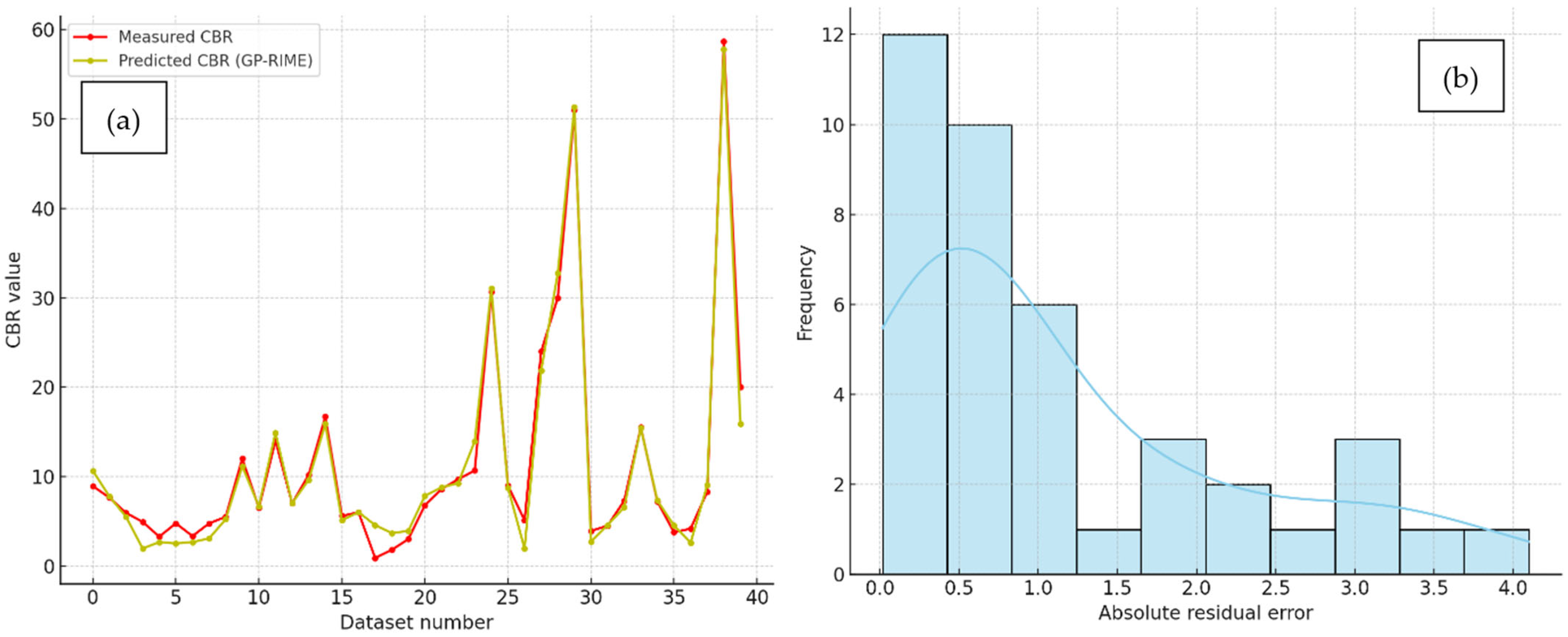
Figure A7 demonstrates the outstanding performance of the GP-RIME in predicting CBR values, with results comparable to the GP-OOA model (Figure A5) and significantly better than the GP-DOA (Figure A3) and MLR (Figure A1) models. Figure A7a shows a near-perfect match between the measured and predicted CBR values across the database, with the predicted values closely following the measured trends. Even at the highest CBR values, the GP-RIME model maintains its accuracy and shows minimal deviations. This high level of alignment highlights the model’s ability to effectively handle both linear and nonlinear relationships in the data, similar to GP-OOA, and vastly superior to the inconsistencies observed with GP-DOA and MLR.
The histogram of absolute residuals in Figure A7b further supports the superior performance of the GP-RIME model. The residuals are tightly clustered around lower values, with most errors below 1 and demonstrate high precision in predictions. The distribution is concentrated towards the lower end, with a rapid decline in frequency for larger errors, showing a narrow and well-contained range of residuals. These results highlight that the GP-RIME model not only achieves results close to GP-OOA but also surpasses GP-DOA and MLR by significantly reducing prediction errors and improving generalisation and makes it one of the most reliable and effective models for this database.
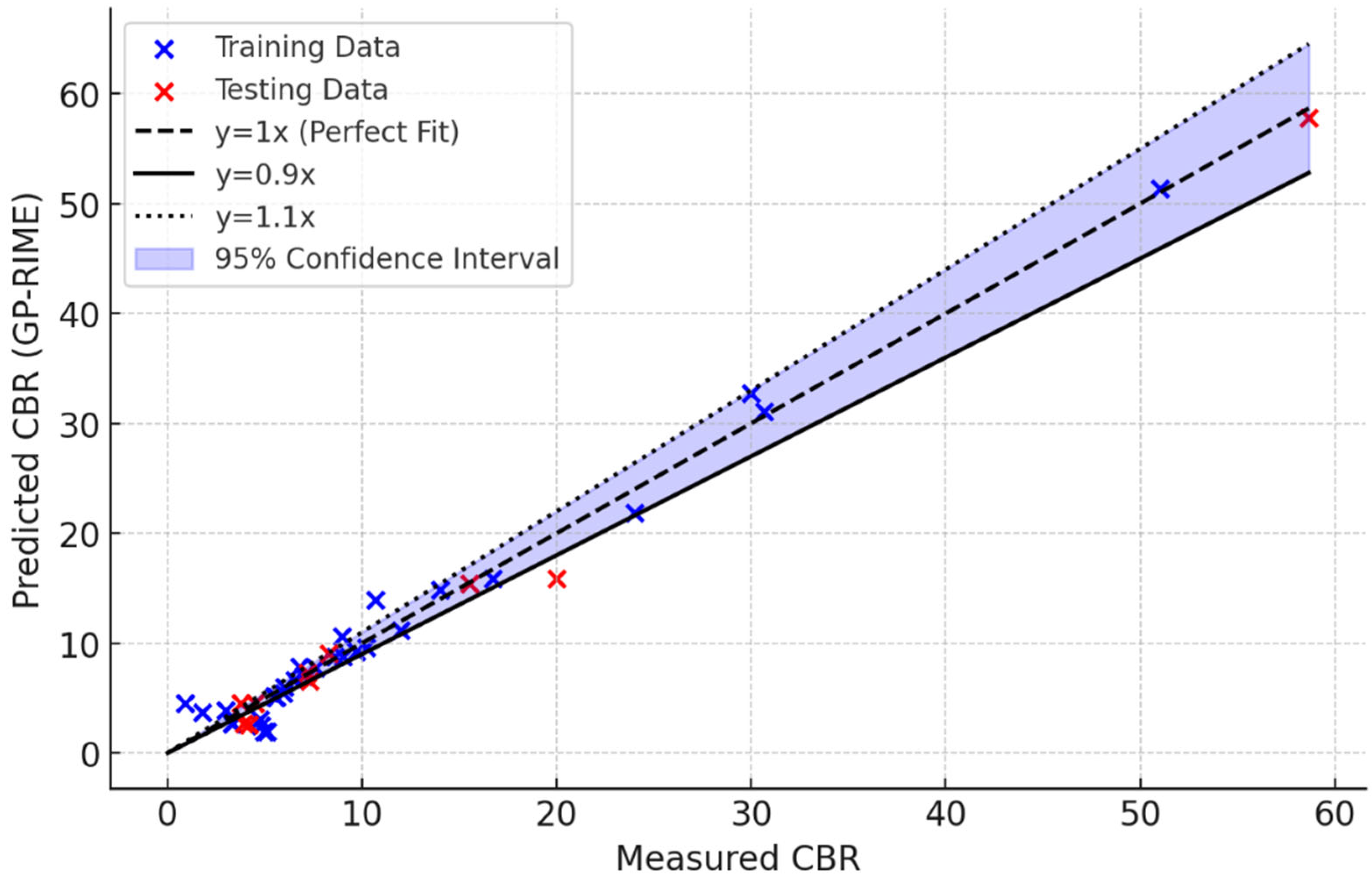
The scatter plot showcases the exceptional performance of the GP-RIME in predicting CBR values for both training and testing databases (Figure A8). The predicted values closely align with the measured values, as evidenced by the tight clustering of points around the perfect fit line (y = 1x). The majority of points fall well within the 10% deviation bounds (y = 0.9x and y = 1.1x), demonstrating high prediction accuracy. The 95% confidence interval is narrow, even at higher CBR values, and reflects the model’s consistency and reliability across a wide range of data. Compared to previous models, GP-RIME excels in maintaining minimal deviations and offers superior generalisation and making it highly effective for accurate and precise predictions in complex databases.
The following formula is the outcome of the GP-RIME model to predict CBR. In Equation (12), all input parameters are normalised values from 0 to 1 based on Equation (12).
C B R = ( ( ( ( X 5 2 r 1 2 ) 2 + X 6 + X 7 ) ( ( X 1 4 ( 2 X 8 r 1 X 7 ) ) ( ( X 6 + X 5 ) ( X 6 + X 7 ) + ( X 7 + X 6 ) ( X 7 + X 5 ) ) ) ) ( X 3 ( X 3 + r 1 ) X 9 r 2 + r 1 2 + X 2 2 ( r 1 X 8 X 5 2 + X 4 ( X 8 + X 1 ) ) ) ) ,
where X1, X2, X3, X4, X5, X6, X7, X8, X9, X10 are soil, sludge, cement, lime content, LL-Soil, PI-Soil Compaction-No. of Hammer (NH), OMC-Mix, MDD-Mix, Gs-Soil, respectively.
Also, r1 and r2 are constants and equal to 0.261 and 0.8445, respectively.
The performance metrics for the GP-RIME model (as shown in Table 12) highlight its exceptional accuracy and reliability, with results closely matching the GP-OOA model and outperforming GP-DOA and MLR models. The MAE is remarkably low at 1.167 for training and 1.019 for testing and indicates precise predictions across both databases. The MSE and RMSE values are also minimal, with 2.530 and 1.591 for training, and 2.313 and 1.521 for testing and demonstrating the model’s ability to minimise errors effectively. The R2 values are 0.977 for training and an impressive 0.991 for testing, and show that the GP-RIME model explains nearly all the variability in the data and generalises exceptionally well to unseen data. These metrics confirm the GP-RIME model’s superiority and make it a highly effective tool for predicting CBR values with unparalleled accuracy.

6. Discussion

6.1. Interpretation, Limitations, and Implications

The nested-CV analysis indicates that nonlinear ensemble modelling (Gradient Boosting) offers robust generalisation on this dataset, while linear regularisation (Ridge) is sensitive to fold composition and fails on at least one split, consistent with nonlinearity in the CBR response. The permutation test supports that the predictive signal is not an artefact of chance correlations (p ≈ 0.005).
Given the small-n regime, two caveats apply. First, reported dispersion (±SD over five outer folds) reflects sampling variability; future expansions of the dataset would further stabilise estimates and tighten uncertainty. Second, the study currently targets the unsoaked CBR response; extension to soaked CBR is recommended to align with conservative pavement design scenarios. Despite these constraints, the combined nested-CV + permutation framework provides a defensible, small-sample validation that directly addresses overfitting concerns.

6.2. Comparison of Models

Distribution of residuals (actual minus predicted values) for four models: MLR, GP-DOA, GP-OOA, and GP-RIME are plotted and presented in Figure 17. The residuals for the MLR model exhibit a wider spread and indicate higher variability and lower predictive accuracy compared to the other models. In contrast, the residuals for GP-DOA, GP-OOA, and GP-RIME are much more concentrated around zero and reflect their superior performance. Among these, GP-RIME shows the most tightly clustered residuals and suggests it achieves the highest prediction accuracy with minimal errors. The narrower and more symmetrical distributions for GP-OOA and GP-RIME highlight their ability to generalise better and provide consistent results and outperform both GP-DOA and MLR. This comparison confirms that the advanced optimisation algorithms (GP-OOA and GP-RIME) significantly enhance prediction reliability over traditional MLR models.
Figure 18 compares the performance of MLR, GP-DOA, GP-OOA, and GP-RIME models in predicting CBR values for both training and testing databases. In the training data comparison, it is evident that all models follow the actual CBR trends to varying degrees. However, the MLR model shows noticeable deviations from the actual values, particularly at higher CBR points and indicates its inability to capture complex patterns effectively. On the other hand, the advanced models (GP-DOA, GP-OOA, and GP-RIME) demonstrate significantly better alignment with the actual CBR values, with GP-RIME achieving the closest match. These results highlight the enhanced predictive capabilities of optimisation-based models compared to traditional regression.
The testing data comparison further emphasises the differences between these models. The MLR model again struggles to generalise and show larger deviations from the actual CBR values, particularly at peak points. In contrast, the GP-DOA, GP-OOA, and GP-RIME models maintain a close match with the actual values, showcasing their robustness in handling unseen data. Among the advanced models, GP-RIME consistently exhibits the most accurate predictions and reinforces its superior generalisation ability.
The correlation heatmap in Figure 19 illustrates the relationships between actual CBR values and the predictions from various models, including MLR, GP-DOA, GP-OOA, and GP-RIME. The GP-based models (GP-DOA, GP-OOA, and GP-RIME) show significantly higher correlations with the actual CBR values (0.98–0.99) compared to the MLR model (0.82), indicating their superior predictive performance. Among the GP-based models, GP-OOA and GP-RIME exhibit the strongest correlations with the actual CBR values (0.99) and reflect their exceptional accuracy and reliability. Furthermore, the intercorrelations among the GP-based models are also very high (0.98–0.99), demonstrating their consistency in capturing complex patterns in the data. In contrast, the MLR model shows weaker correlations with both the actual CBR values and the other models, emphasising its limitations compared to advanced optimisation-based approaches. This heatmap highlights the effectiveness of GP-based models, particularly GP-OOA and GP-RIME, in accurately predicting CBR values.

6.3. Feature Importance

The feature importance for the different models (MLR, GP-DOA, GP-OOA, and GP-RIME) was calculated using distinct approaches based on the characteristics of each model. For MLR, the absolute values of the regression coefficients were normalised to determine their contribution to predicting CBR. For the GP-based models (DOA, OOA, and RIME), sensitivity analysis was performed by evaluating the contribution of each input variable to the predicted CBR values. The MAE approach was applied to estimate the relative influence of each feature by assessing the changes in model outputs when specific input variables were varied. These normalised contributions were used to compute the percentage importance of each parameter and ensured consistent comparisons across models.
Figure 20 shows significant differences in feature importance across the models. For the MLR model, soil content emerged as the most important feature, contributing 36.6% to the predictions, followed by LL-Soil and MDD-Mix. For the GP-DOA and GP-OOA models, LL-Soil and soil content had the highest importance. Interestingly, the GP-RIME model gave the highest weight to soil content and contributed over 45%, while other features like LL-Soil and MDD-Mix also had notable contributions. Across all models, features like cement content, OMC-Mix, and compaction-No. of Hammer (NH) were consistently less influential, though their relative importance varied. These results highlight the differing sensitivities of models to input parameters, reflecting their unique algorithms and prediction mechanisms. This also indicates that certain parameters, such as soil content and LL-Soil, play a fundamental role in prediction accuracy, making them key variables for consideration in future studies.

6.4. a20 Index Evaluation

To further assess the accuracy of the developed models, the a20 index was employed in addition to conventional metrics such as RMSE and R2. The a20 index represents the percentage of predictions that fall within ±20% of the actual values. This metric is increasingly used in recent literature for its practical interpretability in engineering contexts, especially where approximate tolerance thresholds are acceptable [54,55,56]. Table 13 summarises the a20 index values for all four models considered in this study.
The results show that the a20 index improves significantly across the models, with the traditional Multiple Linear Regression (MLR) model achieving the lowest value (37.5%). In contrast, the GP-RIME model achieved the highest accuracy, with 70.0% of its predictions falling within a ±20% deviation from the actual CBR values. The progressive improvement across GP-DOA (47.5%), GP-OOA (60.0%), and GP-RIME (70.0%) highlights the strength of integrating genetic programming with metaheuristic algorithms in capturing complex, nonlinear soil behaviour. These findings support the suitability of the GP-RIME model for reliable and interpretable geotechnical predictions.

6.5. Prediction-Interval Calibration (95% PI)

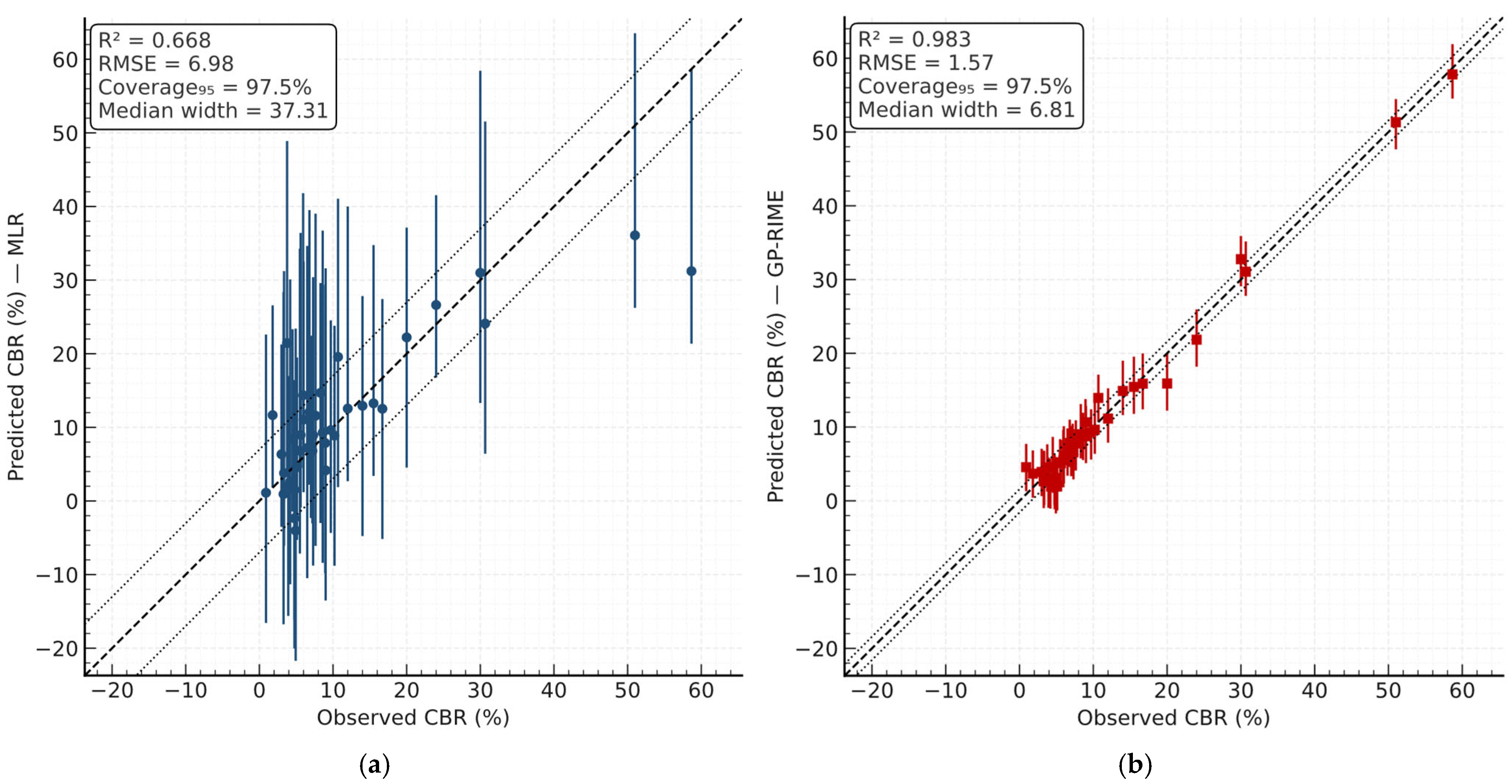
Figure 21 shows the parity plot with 95% PIs for the multiple linear regression (MLR) model. GP-based models (GP-RIME, GP-OOA, GP-DOA; including second independent runs) demonstrate substantially narrower intervals at near-nominal coverage; their plots are provided in Figure 21, Figure 22 and Figure 23. Table 14 summarises coverage and interval width for all models.
Across the updated dataset, coverage values are close to the nominal 95% for all models, while interval widths vary by model family: GP variants concentrate uncertainty more tightly (median 6–9 CBR %), in contrast to MLR (≈33 CBR %), consistent with the higher flexibility of symbolic GP expressions under similar residual variability. This behaviour is also visible in the width–prediction profiles, where GP intervals remain comparatively stable across the prediction range.

6.6. Comparative Context with Prior Studies

The untreated soil in this study had CBR = 9.0. Optimum mix achieved CBR = 58.7 (≈550% increase), using cement+lime under the selected compaction effort. Recent work on aluminium-based WTS in subgrade applications reported an optimum CBR of 41.50% at 5% WTS for soil–WTS–cement mixtures, and 21.25% at 15% WTS for soil–WTS–lime mixtures [57]. These values are broadly consistent with findings of this study that cement and lime together can deliver higher CBR than lime alone at comparable or lower WTS contents; differences in absolute values reflect variations in soil type, WTS source and dosage, binder contents, and compaction procedures across studies.
In the experiments, the optimum moisture content increased by ~18% while the maximum dry density decreased by ~9% with WTS addition. This trend aligns with published observations for WTS-stabilised mixtures, where higher water demand and the lower specific gravity/porosity of WTS shift the compaction curve (higher OMC, lower MDD).
Sensitivity analysis of this study indicates compaction effort (number of blows) is a dominant predictor of CBR. This agrees with prior AI-based studies on alum-sludge–stabilised soils, which identify compaction energy as a top-ranked factor controlling predicted CBR, ahead of several mix descriptors.
Although previous AI applications (for example, Random Forest, ANN, gradient boosting) have shown predictive potential for soil and interface behaviour, they remain largely black-box approaches with limited interpretability and without explicit physics-awareness. On the other hand, classical Mohr–Coulomb and linear regression models are too simplistic to represent the nonlinear, multivariate interactions inherent in soil–structure interfaces. To date, no study has bridged this gap by developing an interpretable, physics-informed symbolic regression framework that not only enhances predictive accuracy but also produces transparent formulas consistent with fundamental geotechnical principles. This study addresses this gap by proposing a hybrid GP framework that integrates SHAP-guided feature selection, Fourier feature augmentation, and physics-informed constraints. Table 15 shows a summary comparison of CBR outcomes for WTS-stabilised soils.

6.7. Collinearity, Proxies, and Mechanisms

Mechanistic behaviour is inferred directly from the interaction partial dependence [58,59,60,61] in Figure 24 (LL-Soil × Lime Content). The response surface shows that higher LL-Soil is associated with lower CBR when lime content is low, indicating a fines-dominated, moisture-sensitive matrix that limits stiffness. As lime content increases, the adverse influence of LL-Soil progressively attenuates, and the surface flattens toward a higher-CBR regime—consistent with flocculation and early pozzolanic bonding that reorganise the microstructure and stiffen the skeleton despite active fines.

6.8. Limitations

While this study provides valuable insights into the use of water treatment sludge (WTS) combined with soil, cement, and lime for subgrade stabilisation, several limitations should be acknowledged. First, the experimental program was based on a relatively small dataset (40 observations), which may limit the generalisability of the predictive models. Although cross-validation and performance metrics suggest strong model accuracy, larger and more diverse datasets would further strengthen the robustness of the results. Second, only unsoaked CBR conditions were evaluated; future work should include soaked CBR and long-term durability tests under field-like environmental cycles (for example, wetting–drying or freeze–thaw). Third, the study used a single source of alum-based WTS, and variations in sludge composition from different treatment plants were not considered.
For the machine learning models, the limited sample size, though enhanced by combining experimental and published data, remains a constraint. To reduce the risk of overfitting, the modelling framework incorporated multiple train-test splits, several statistical metrics (R2, RMSE, MAE, and a20), and interpretable genetic programming techniques. However, to ensure greater generalisation across diverse geotechnical conditions, future work should aim to expand the dataset with more varied soil types, sludge sources, and mix designs.
The scope is restricted to unsoaked response; under soaking, stabilised matrices can exhibit reduced CBR due to loss of matric suction, softening of the fines skeleton, and altered lime–clay interactions. To address this, future work will measure 4-day soaked CBR on identical mix designs and compaction energies, quantify unsoaked-to-soaked differentials, and extend the predictive framework to incorporate moisture state so that design-relevant soaked performance can be estimated with appropriate uncertainty.

7. Conclusions

This study demonstrates the transformative potential of water treatment sludge (WTS) as a sustainable material for soil stabilisation when combined with soil, cement, and lime. The experimental results revealed that mixtures incorporating WTS significantly enhance California Bearing Ratio (CBR) values, a critical indicator of subgrade strength and load-bearing capacity. The optimal mixture of 40% soil, 50% sludge and 10% lime achieved a remarkable CBR value of 58.7 and reflected a 550% improvement compared to untreated soil (CBR = 9.0).
The study also revealed significant improvements in compaction characteristics due to the addition of WTS. The optimum moisture content (OMC) of the mixtures increased by approximately 18%, while the maximum dry density (MDD) decreased by 9% and highlighted the lightweight nature of WTS. This reduction in density, combined with enhanced CBR values, makes WTS an efficient and environmentally friendly stabilising agent. These results show the feasibility of integrating WTS into geotechnical applications to replace conventional materials and reduce both construction costs and environmental impacts associated with sludge disposal.
Advanced modelling using explainable metaheuristic-based genetic programming (GP) validated the experimental findings and provided insights into the complex relationships between mixture components. Among the tested models, the GP-RIME model achieved the highest predictive accuracy, with an R2 of 0.991 and a mean absolute error (MAE) of 1.02. Similarly, the GP-OOA model performed exceptionally well and achieved an R2 of 0.989 and an MAE of 1.19. These models significantly outperformed traditional multiple linear regression (R2 = 0.552, MAE = 6.53) and demonstrated their ability to handle nonlinear relationships and heterogeneous material behaviours effectively.
Feature importance analysis revealed the relative contributions of the mixture components to the CBR predictions. The results revealed that soil content, LL-Soil, and MDD-Mix are the most influential parameters across all models, with soil content being the dominant feature, particularly in the GP-RIME model where it exceeds 45% importance. Sludge content and PI-Soil also showed moderate significance, especially in certain models like GP-DOA and GP-OOA. In contrast, cement content, OMC-Mix, lime content, and compaction-No. of Hammer (NH) consistently exhibited lower importance, indicating that these parameters contribute less to the predictive performance of the models.
The findings of this study are particularly significant for advancing sustainable construction practices. By recycling WTS into soil stabilisation applications, the dual benefits of waste reduction and improved subgrade performance can be achieved. This approach aligns with circular economy principles and reduces landfill pressure and minimises the environmental footprint of construction projects. Additionally, the ability to tailor the proportions of soil, sludge, cement, and lime to meet specific performance criteria provides a flexible and cost-effective solution for various geotechnical applications, particularly in road construction and pavement subgrades.
Future research should focus on field validation of these findings to evaluate the long-term durability and performance of WTS-based mixtures under real-world conditions. Investigating the scalability and economic feasibility of these mixtures in large infrastructure projects would further strengthen their applicability. Moreover, developing standardised guidelines for incorporating WTS into subgrade design and testing the effectiveness of other waste materials in combination with WTS could pave the way for broader adoption of sustainable and innovative material recycling in construction. This study establishes a strong foundation for integrating experimental research, advanced modelling, and sustainability in geotechnical engineering. The conclusions are limited to unsoaked performance. Given that soaked CBR commonly governs conservative pavement design, these results should be applied with caution and not used as proxies for soaked behaviour.
Beyond technical performance, the findings highlight the environmental significance of adopting WTS as a sustainable stabilisation agent. By transforming a waste by-product into a functional construction material, this study demonstrates a pathway toward more sustainable and resource-efficient ground improvement practices. Wider adoption could contribute to reduced waste disposal, lower CO2 emissions from lime and cement production, and alignment with the UN Sustainable Development Goals.

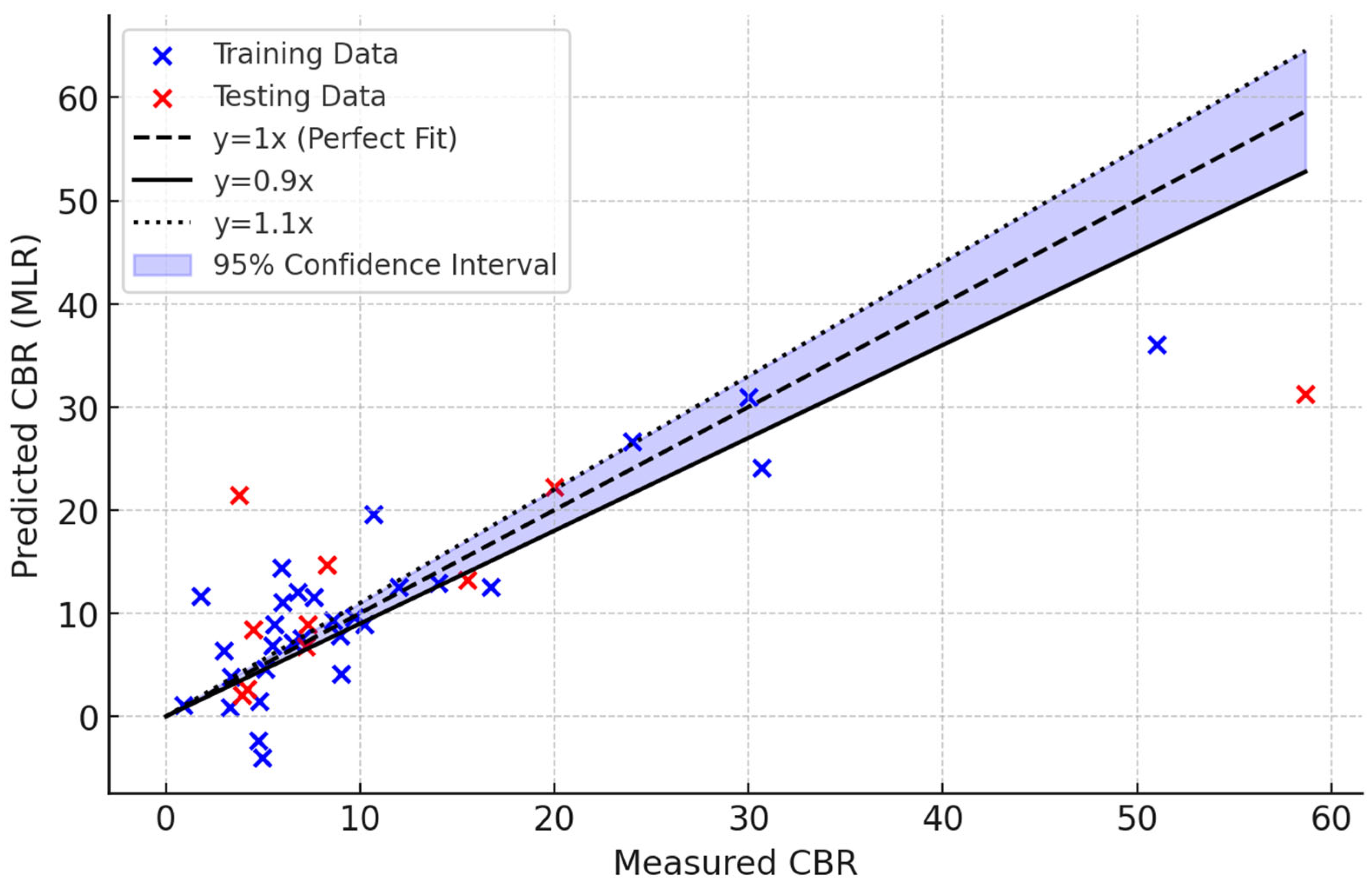
Author Contributions

Conceptualisation, B.K. and A.B.; methodology, B.K. and A.B.; software, A.B.; validation, B.K.; formal analysis, B.K.; investigation, B.K. and A.B.; resources, B.K. and A.B.; data curation, A.B.; writing—original draft preparation, B.K. and A.B.; writing—review and editing, B.K. and A.B.; visualisation, A.B.; supervision, B.K.; project administration, B.K. and A.B.; funding acquisition, B.K. All authors have read and agreed to the published version of the manuscript.

Funding

This research received no external funding.

Institutional Review Board Statement

Not applicable.

Informed Consent Statement

Not applicable.

Data Availability Statement

The data are attached in Appendix C.

Acknowledgments

The authors express their gratitude to Navya Maria Titus, Samandeep Kaur, and Taj Dillon for their support during experimental work. They also thank the laboratory staff at the School of Engineering, Deakin University, for their help in setting up lab equipment for experimentation. The authors greatly acknowledge the support from Barwon Water for providing the necessary sludge waste from their treatment facility for this study.

Conflicts of Interest

The authors declare no conflicts of interest.

Abbreviations

The following abbreviations are used in this manuscript:
WTSWater Treatment Sludge
CBRCalifornia Bearing Ratio
GPGenetic Programming
DOADingo Optimisation Algorithm
OOAOsprey Optimisation Algorithm
RIMERime-Ice Optimisatino Algorithm
MAEMean Absolute Error
SHAPSHapley Additive exPlanations
ITSIndirect Tensile Strength
UCSUnconfined Compressive Strength
MLRMultiple Linear Regression

Appendix A

Figure A1. Performance evaluation of MLR model: (a) Predicted vs. measured CBR values and (b) residual error distribution.
Sustainability 17 09919 g0a1
Figure A2. Predicted CBR values by MLR model.
Sustainability 17 09919 g0a2
Figure A3. Performance evaluation of GP-DOA model: (a) Predicted vs. measured CBR values and (b) residual error distribution.
Sustainability 17 09919 g0a3
Figure A4. Predicted CBR values by GP-DOA model.
Sustainability 17 09919 g0a4
Figure A5. Performance evaluation of GP-OOA model: (a) Predicted vs. measured CBR values and (b) residual error distribution.
Sustainability 17 09919 g0a5
Figure A6. Predicted CBR values by GP-OOA model.
Sustainability 17 09919 g0a6
Figure A7. Performance evaluation of GP-RIME model: (a) Predicted vs. measured CBR values and (b) residual error distribution.
Sustainability 17 09919 g0a7
Figure A8. Predicted CBR values by GP-RIME model.
Sustainability 17 09919 g0a8

Appendix B. Model Parameters

Table A1. Recommended genetic-programming hyperparameters for the GP-OOA.
ParameterValue
Population750
Generations300
SelectionTournament (k = 7)
Elitism2
Crossover0.85
Mutation0.12
Reproduction0.03
Max initial level2–6 (ramped half-and-half)
Max depth (ops)10
Brood size6
FitnessRMSE (secondary: a20)
Early stopping25 rounds, val split 0.15
NormalisationMin–max
ERC (random constants)range [0, 1], count 8
Function set +, −, *, pow2
Table A2. Recommended genetic-programming hyperparameters for the GP-DOA.
ParameterValue
Population600
Generations300
SelectionRank (value = 1.6)
Elitism1
Crossover0.86
Mutation0.10
Reproduction0.04
Max initial level2–6 (ramped half-and-half)
Max depth (ops)10
Brood size6
FitnessRMSE
Early stopping25 rounds, val split 0.15
NormalisationMin–max
ERC (random constants)range [0, 1], count 8
Function set +, −, *, pow2
Table A3. Recommended genetic-programming hyperparameters for the GP-RIME.
ParameterValue
Population800
Generations300
SelectionTournament (k = 7)
Elitism2
Crossover0.84
Mutation0.13
Reproduction0.03
Max initial level2–6 (ramped half-and-half)
Max depth (ops)10
Brood size6
FitnessRMSE (secondary: a20)
Early stopping25 rounds, val split 0.15
NormalisationMin–max
ERC (random constants)range [0, 1], count 8
Function set +, −, *, pow2

Appendix C. Database

Table A4. Database: Inputs.
DatabasesNo.Soil ContentSludge ContentCement ContentLime ContentLL-SoilPI-SoilCompaction-No. of Hammer (NH)OMC-MixMDD-MixGs-Soil
Training Database10902.57.50025400.8820
2090550025390.8920
30907.52.5002540.50.8880
40100000025400.8540
59550027.288.8325201.422.17
785150027.288.8325221.452.17
875250027.288.8325221.452.17
910000027.288.8325181.562.17
1198200553410211.61792.75
1398200553465211.61792.75
1496400553410191.66592.75
1596400553465191.66592.75
169460055341018.51.68192.75
1992800553430181.7462.75
2092800553465181.7462.75
2190100055341022.51.56982.75
2290100055343022.51.56982.75
2310000040.2820.2325191.7252.7
2450500032.4914.142526.51.4452.7
2710000055341022.51.58582.75
2810000055346522.51.58582.75
2996400553430191.66592.75
309460055343018.51.68192.75
3250500055.841.2149311.312.53
3345500555.841.214332.41.2952.5
35100000563825191.7752.74
360100000025421.062.74
3838602056382536.71.212.74
3936604056382538.41.2012.74
4034606056382536.51.242.74
Testing Database690100027.288.8325201.422.17
1010000055343022.51.58582.75
1298200553430211.61792.75
179460055346518.51.68192.75
1892800553410181.7462.75
2501000026.129.112541.51.062.7
2680200027.288.8325221.452.17
3190100055346522.51.56982.75
34405001055.841.216733.61.3082.47
3740600056382535.11.2182.74
Table A5. Database: Outputs.
No.Actual CBRGP-OOAGP-DOAGP-RIME
18.946.7752096.9717901810.64782242
27.636.7752098.0282569137.769689962
35.946.7752097.5462843915.499095302
44.936.7752095.2737708751.953880343
53.2796.7661245312.3578944232.674145023
74.7726.7359459422.2635076792.520186912
83.3476.7518043872.3178990832.679790125
94.766.7752092.453132173.078824722
115.56.7752096.4805258495.222051337
13128.207851548.98243762511.1536996
146.56.7752098.2945330146.670018362
151410.9413649513.9282581814.89522431
1676.7752098.6920879017.016681222
1910.29.3465809629.045696529.643809002
2016.715.6791838416.9631366615.87806711
215.66.7752095.625002575.110346715
2267.2048715955.6303621026.023465107
230.96.7752093.9295895074.566424647
241.86.7855829992.9643494243.686688567
2736.7752094.7742182613.913425412
286.86.7752095.8978427267.849931944
298.67.8024665878.2899150878.794145223
309.78.5240971258.6910267649.259034075
3210.6814.3795637112.8695280613.95318769
3330.6630.2623661930.1946987531.06264296
3596.7752099.929578688.764233189
365.16.7752094.6502139561.953880343
382421.8146926225.4039127221.84836633
393034.1945093931.6028837132.75927853
405151.4490028550.4164906151.32370359
63.9236.7630951642.3685148812.717519241
104.56.7752094.7786127564.571814038
127.36.9643662946.4775499696.568054344
1715.513.2745138315.4126351915.45041615
187.26.7752099.0400735437.30960437
253.763.1611438373.8167971564.520479029
264.1786.7419835832.2907033812.606099998
318.311.545828596.9953767019.025915732
3458.6757.8727356458.5514378857.80554882
372017.309425216.1018739715.90156422

References

  1. Tanyildizi, M.; Uz, V.E.; Gokalp, I. Utilization of waste materials in the stabilization of expansive pavement subgrade: An extensive review. Constr. Build. Mater. 2023, 398, 132435. [Google Scholar] [CrossRef]
  2. Baghbani, A.; Kiany, K.; Abuel-Naga, H.; Lu, Y. Predicting the compression index of clayey soils using a hybrid genetic programming and xgboost model. Appl. Sci. 2025, 15, 1926. [Google Scholar] [CrossRef]
  3. Lu, Y.; Xu, C.; Baghbani, A. Initial state of excavated soil and rock (ESR) to influence the stabilisation with cement. Constr. Build. Mater. 2023, 400, 132879. [Google Scholar] [CrossRef]
  4. Vishnu, T.B.; Singh, K.L. A study on the suitability of solid waste materials in pavement construction: A review. Int. J. Pavement Res. Technol. 2021, 14, 625–637. [Google Scholar] [CrossRef]
  5. Zhou, C.; Richardson-Barlow, C.; Fan, L.; Cai, H.; Zhang, W.; Zhang, Z. Towards organic collaborative governance for a more sustainable environment: Evolutionary game analysis within the policy implementation of China’s net-zero emissions goals. J. Environ. Manag. 2025, 373, 123765. [Google Scholar] [CrossRef]
  6. Lucena, L.C.D.F.L.; Juca, J.F.T.; Soares, J.B.; Marinho Filho, P.G.T. Use of wastewater sludge for base and subbase of road pavements. Transp. Res. Part D Transp. Environ. 2014, 33, 210–219. [Google Scholar] [CrossRef]
  7. Kafle, B.; Baghbani, A.; Pempeit, R.; Shrestha, K. Investigating the Mechanical Behaviour of Unbound Granular Material (UGM) for Road Pavement Construction Applications: A Western Victoria Case Study. Int. J. Geosynth. Ground Eng. 2024, 10, 29. [Google Scholar] [CrossRef]
  8. Kiany, K.; Baghbani, A.; Abuel-Naga, H.; Yi, L. Novel integration of FEM, Physics-Informed Neural Networks, and explainable Metaheuristics for retaining wall analysis. Int. J. Geotech. Eng. 2025, 19, 813–831. [Google Scholar] [CrossRef]
  9. Hubballi, R.M.; Rahman, S.K. Soil Improvement Using Coir Fibre: A Case Study. Int. J. Adv. Res. Eng. Technol. (IJARET) 2021, 12, 593–598. [Google Scholar]
  10. Gupta, C.; Sharma, R.K. Black cotton soil modification by the application of waste materials. Period. Polytech. Civ. Eng. 2016, 60, 479–490. [Google Scholar] [CrossRef]
  11. Cabalar, A.F.; Hassan, D.I.; Abdulnafaa, M.D. Use of waste ceramic tiles for road pavement subgrade. Road Mater. Pavement Des. 2017, 18, 882–896. [Google Scholar] [CrossRef]
  12. Ahmad, J.; Kontoleon, K.J.; Majdi, A.; Naqash, M.T.; Deifalla, A.F.; Ben Kahla, N.; Isleem, H.F.; Qaidi, S.M. A comprehensive review on the ground granulated blast furnace slag (GGBS) in concrete production. Sustainability 2022, 14, 8783. [Google Scholar] [CrossRef]
  13. Amakye, S.Y.; Abbey, S.J.; Booth, C.A.; Mahamadu, A.M. Enhancing the engineering properties of subgrade materials using processed waste: A review. Geotechnics 2021, 1, 307–329. [Google Scholar] [CrossRef]
  14. Deboucha, S.; Aissa Mamoune, S.M.; Sail, Y.; Ziani, H. Effects of ceramic waste, marble dust, and cement in pavement sub-base layer. Geotech. Geol. Eng. 2020, 38, 3331–3340. [Google Scholar] [CrossRef]
  15. Sharma, R.K. Utilization of fly ash and waste ceramic in improving characteristics of clayey soil: A laboratory study. Geotech. Geol. Eng. 2020, 38, 5327–5340. [Google Scholar] [CrossRef]
  16. Baghbani, A.; Faradonbeh, R.S.; Lu, Y.; Soltani, A.; Kiany, K.; Baghbani, H.; Abuel-Naga, H.; Samui, P. Enhancing earth dam slope stability prediction with integrated AI and statistical models. Appl. Soft Comput. 2024, 164, 111999. [Google Scholar] [CrossRef]
  17. Monkman, S.; Hanmore, A.; Thomas, M. Sustainability and durability of concrete produced with CO2 beneficiated reclaimed water. Mater. Struct. 2022, 55, 170. [Google Scholar] [CrossRef]
  18. Nia, S.B.; Chari, M.N. Applied development of sustainable-durable high-performance lightweight concrete: Toward low carbon footprint, durability, and energy saving. Results Mater. 2023, 20, 100482. [Google Scholar]
  19. Liu, Y.; Zhuge, Y.; Chow, C.W.; Keegan, A.; Pham, P.N.; Li, D.; Qian, G.; Wang, L. Recycling drinking water treatment sludge into eco-concrete blocks with CO2 curing: Durability and leachability. Sci. Total Environ. 2020, 746, 141182. [Google Scholar] [CrossRef]
  20. Yagüe, A.; Valls, S.; Vázquez, E.; Albareda, F. Durability of concrete with addition of dry sludge from waste water treatment plants. Cem. Concr. Res. 2005, 35, 1064–1073. [Google Scholar] [CrossRef]
  21. Mojapelo, K.S.; Kupolati, W.K.; Burger, E.A.; Ndambuki, J.M.; Snyman, J.; Achi, C.G.; Quadri, A.I. Durability and Environmental Impact of Wastewater Sludge Ash as a Cement Replacement in Concrete: Challenges and Future Directions. Mater. Circ. Econ. 2025, 7, 15. [Google Scholar] [CrossRef]
  22. Pham, P.N.; Duan, W.; Zhuge, Y.; Liu, Y.; Tormo, I.E.S. Properties of mortar incorporating untreated and treated drinking water treatment sludge. Constr. Build. Mater. 2021, 280, 122558. [Google Scholar] [CrossRef]
  23. Marchiori, L.; Albuquerque, A.; Cavaleiro, V. Water Treatment Sludge as Geotechnical Liner Material: State-of-Art. In Proceedings of the International Conference on Environmental Geotechnology, Recycled Waste Materials and Sustainable Engineering, Jalandhar, India, 25–27 October 2023; Springer: Singapore, 2023; pp. 529–547. [Google Scholar]
  24. Abo-El-Enein, S.A.; Shebl, A.; El-Dahab, S.A. Drinking water treatment sludge as an efficient adsorbent for heavy metals removal. Appl. Clay Sci. 2017, 146, 343–349. [Google Scholar] [CrossRef]
  25. Nguyen, M.D.; Baghbani, A.; Alnedawi, A.; Ullah, S.; Kafle, B.; Thomas, M.; Moon, E.M.; Milne, N.A. Investigation on the suitability of aluminium-based water treatment sludge as a sustainable soil replacement for road construction. Transp. Eng. 2023, 12, 100175. [Google Scholar] [CrossRef]
  26. Nguyen, M.D.; Thomas, M.; Surapaneni, A.; Moon, E.M.; Milne, N.A. Beneficial reuse of water treatment sludge in the context of circular economy. Environ. Technol. Innov. 2022, 28, 102651. [Google Scholar] [CrossRef]
  27. Baghbani, A.; Nguyen, M.D.; Kafle, B.; Baghbani, H.; Shirani Faradonbeh, R. AI grey box model for alum sludge as a soil stabilizer: An accurate predictive tool. Int. J. Geotech. Eng. 2023, 17, 480–494. [Google Scholar] [CrossRef]
  28. Baghbani, A.; Abuel-Naga, H.; Shirkavand, D. Accurately predicting quartz sand thermal conductivity using machine learning and grey-box AI models. Geotechnics 2023, 3, 638–660. [Google Scholar] [CrossRef]
  29. Dahhou, M.; El Hamidi, A.; El Moussaouiti, M. Reusing drinking water sludge: Physicochemical features, environmental impact and applications in building materials: A mini review. Chem. Afr. 2023, 6, 1145–1161. [Google Scholar] [CrossRef]
  30. Balkıs, A.; Macid, S. Effect of cement amount on CBR values of different soil. Avrupa Bilim Teknol. Derg. 2019, 2019, 809–815. [Google Scholar]
  31. Baghbani, A.; Soltani, A.; Kiany, K.; Daghistani, F. Predicting the strength performance of hydrated-lime activated rice husk ash-treated soil using two grey-box machine learning models. Geotechnics 2023, 3, 894–920. [Google Scholar] [CrossRef]
  32. Malkanthi, S.N.; Balthazaar, N.; Perera, A.A.D.A.J. Lime stabilization for compressed stabilized earth blocks with reduced clay and silt. Case Stud. Constr. Mater. 2020, 12, 00326. [Google Scholar] [CrossRef]
  33. Dhar, S.; Hussain, M. The strength and microstructural behavior of lime stabilized subgrade soil in road construction. Int. J. Geotech. Eng. 2021, 15, 471–483. [Google Scholar] [CrossRef]
  34. Armaghani, D.J.; Yang, P.; He, X.; Pradhan, B.; Zhou, J.; Sheng, D. Toward Precise Long-Term Rockburst Forecasting: A Fusion of SVM and Cutting-Edge Meta-heuristic Algorithms. Nat. Resour. Res. 2024, 33, 2037–2062. [Google Scholar] [CrossRef]
  35. Phan, V.H.; Ly, H.B. RIME-RF-RIME: A novel machine learning approach with SHAP analysis for predicting macroscopic permeability of porous media. J. Sci. Transp. Technol. 2024, 4, 58–71. [Google Scholar] [CrossRef]
  36. AS 1289.3.6.1-2009; Methods of Testing Soils for Engineering Purposes—Method 3.6.1: Soil Classification Tests—Determination of the Particle Size Distribution of a Soil—Standard Method of Analysis by Sieving. Standards Australia: Sydney, Australia, 2009.
  37. AS 1289.3.1.2-2009; Methods of Testing Soils for Engineering Purposes—Method 3.1.2: Determination of the Liquid Limit of a Soil—Four-Point Casagrande Method. Standards Australia: Sydney, Australia, 2009.
  38. AS 1289.3.2.1-2009; Methods of Testing Soils for Engineering Purposes—Method 3.2.1: Determination of the Plastic Limit of a Soil. Standards Australia: Sydney, Australia, 2009.
  39. AS 1289.3.4.1-2008; Methods of Testing Soils for Engineering Purposes—Method 3.4.1: Determination of the Linear Shrinkage of a Soil—Standard Method. Standards Australia: Sydney, Australia, 2008.
  40. AS 1289.5.1.1-2003; Methods of Testing Soils for Engineering Purposes—Method 5.1.1: Compaction Control Test—Standard Compactive Effort. Standards Australia: Sydney, Australia, 2003.
  41. Sainsbury, B.A.; Gharehdash, S.; Sainsbury, D. Large-scale characterisation of cemented rock fill performance for exposure stability analysis. Constr. Build. Mater. 2021, 308, 124995. [Google Scholar] [CrossRef]
  42. Ghadakpour, M.; Janalizadeh Choobbasti, A.; Soleimani Kutanaei, S. Investigation of the deformability properties of fiber reinforced cemented sand. J. Adhes. Sci. Technol. 2019, 33, 1913–1938. [Google Scholar] [CrossRef]
  43. Ferreira, C. Gene Expression Programming: Mathematical Modeling by an Artificial Intelligence; Springer: Berlin/Heidelberg, Germany, 2006; Volume 21. [Google Scholar]
  44. Gandomi, A.H.; Alavi, A.H. A new multi-gene genetic programming approach to nonlinear system modeling. Part I: Materials and structural engineering problems. Neural Comput. Appl. 2012, 21, 171–187. [Google Scholar] [CrossRef]
  45. Mishra, T.; Singh, A.K.; Kamboj, V.K. An improved nature inspired levy dingo optimisation algorithm for multidisciplinary engineering design problems. In AIP Conference Proceedings; AIP Publishing: Melville, NY, USA, 2023; Volume 2800. [Google Scholar]
  46. Yu, Z.; Shao, P.; Zhang, S. Enhanced Dingo Optimisation Algorithm Based on Differential Evolution and Chaotic Mapping for Engineering Optimisation. In International Conference on Swarm Intelligence; Springer Nature: Singapore, 2024; pp. 223–234. [Google Scholar]
  47. Wei, F.; Shi, X.; Feng, Y. Improved osprey optimisation algorithm based on two-color complementary mechanism for global optimisation and engineering problems. Biomimetics 2024, 9, 486. [Google Scholar] [CrossRef]
  48. Arafin, T.; Mridul, M.A.; Sadman, S. Enhancing Efficiency of Affordable Sensors: An Advanced Neural Network Paradigm with Metaheuristic Optimisation Algorithms. Ph.D. Thesis., Department of Electrical and Elecrtonics Engineering (EEE), Islamic University of Technology (IUT), Gazipur, Bangladesh, 2023. [Google Scholar]
  49. He, B.; Armaghani, D.J.; Tsoukalas, M.Z.; Qi, C.; Bhatawdekar, R.M.; Asteris, P.G. A case study of resilient modulus prediction leveraging an explainable metaheuristic-based XGBoost. Transp. Geotech. 2024, 45, 101216. [Google Scholar] [CrossRef]
  50. Su, H.; Zhao, D.; Heidari, A.A.; Liu, L.; Zhang, X.; Mafarja, M.; Chen, H. RIME: A physics-based optimisation. Neurocomputing 2023, 532, 183–214. [Google Scholar] [CrossRef]
  51. Donizetti, A.; Bellosta, T.; Guardone, A. Ice shape convergence in multi-step ice accretion simulations over straight wings. In Proceedings of the AIAA Scitech 2024 Forum, Orlando, FL, USA, 8–12 January 2024; p. 2679. [Google Scholar]
  52. Li, P.; Wang, H.; Tian, G.; Fan, Z. Towards Sustainable Cloud Computing: Load Balancing with Nature-Inspired Meta-Heuristic Algorithms. Electronics 2024, 13, 2578. [Google Scholar] [CrossRef]
  53. Shah, S.A.R.; Mahmood, Z.; Nisar, A.; Aamir, M.; Farid, A.; Waseem, M. Compaction performance analysis of alum sludge waste modified soil. Constr. Build. Mater. 2020, 230, 116953. [Google Scholar] [CrossRef]
  54. Jadhav, P.; Sakpal, S.; Khedekar, H.; Pawar, P.; Malipatil, M. Experimental Investigation of Soil Stabilization by Using Alum Sludge. Int. J. Res. Appl. Sci. Eng. Technol 2022, 10, 598–602. [Google Scholar] [CrossRef]
  55. Ly, H.B.; Pham, B.T.; Le, L.M.; Le, T.T.; Le, V.M.; Asteris, P.G. Estimation of axial load-carrying capacity of concrete-filled steel tubes using surrogate models. Neural Comput. Appl. 2021, 33, 3437–3458. [Google Scholar] [CrossRef]
  56. Tilahun, Y.; Xiao, Q.; Ashango, A.A.; Han, X.; Negewo, M. Prediction of Spatial Soil-California Bearing Ratio of Subgrade Soil Using Particle Swarm Optimization—Artificial Intelligence Method. Transp. Infrastruct. Geotechnol. 2025, 12, 80. [Google Scholar] [CrossRef]
  57. Takao, T.W.; Bardini, V.S.; de Jesus, A.D.; Marchiori, L.; Albuquerque, A.; Fiore, F.A. Beneficial Use of Water Treatment Sludge with Stabilizers for Application in Road Pavements. Sustainability 2024, 16, 5333. [Google Scholar] [CrossRef]
  58. Boscov, M.E.G.; Tsugawa, J.K.; Tejeda Montalvan, E.L. Beneficial Use of Water Treatment Sludge in Geotechnical Applications as a Sustainable Alternative to Preserve Natural Soils. Sustainability 2021, 13, 9848. [Google Scholar] [CrossRef]
  59. Dormann, C.F.; Elith, J.; Bacher, S.; Buchmann, C.; Carl, G.; Carré, G.; Marquéz, J.R.; Gruber, B.; Lafourcade, B.; Leitão, P.J.; et al. Collinearity: A review of methods to deal with it and a simulation study evaluating their performance. Ecography 2013, 36, 27–46. [Google Scholar] [CrossRef]
  60. Schisterman, E.F.; Perkins, N.J.; Mumford, S.L.; Ahrens, K.A.; Mitchell, E.M. Collinearity and causal diagrams: A lesson on the importance of model specification. Epidemiology 2017, 28, 47–53. [Google Scholar] [CrossRef] [PubMed]
  61. Kock, N.; Lynn, G.S. Lateral collinearity and misleading results in variance-based SEM: An illustration and recommendations. J. Assoc. Inf. Syst. 2012, 13, 2. [Google Scholar] [CrossRef]
Figure 1. Study workflow: evaluating alum sludge performance in geotechnical applications.
Sustainability 17 09919 g001
Figure 2. Location map of the sludge stockpile.
Sustainability 17 09919 g002
Figure 3. Alum sludge used in this study.
Sustainability 17 09919 g003
Figure 4. Soil is used in this study.
Sustainability 17 09919 g004
Figure 5. Ordinary Portland cement used in this study.
Sustainability 17 09919 g005
Figure 6. Hydrated lime is used in this study.
Sustainability 17 09919 g006
Figure 7. Particle size distribution: comparison of clay and alum sludge samples.
Sustainability 17 09919 g007
Figure 8. Compaction curves for sludge, soil, cement, and lime mixtures.
Sustainability 17 09919 g008
Figure 9. Load-penetration behaviour of different sludge-soil-cement-lime mixtures.
Sustainability 17 09919 g009
Figure 10. Relationship between sludge content and CBR values for various material compositions.
Sustainability 17 09919 g010
Figure 11. Effect of different parameters on CBR.
Sustainability 17 09919 g011
Figure 12. Effect of OMC and MDD of Mix on CBR values.
Sustainability 17 09919 g012
Figure 13. Boxplot representation of variable distributions for CBR prediction.
Sustainability 17 09919 g013
Figure 14. Histograms with density plots for variable distributions in CBR prediction.
Sustainability 17 09919 g014
Figure 15. Correlation heatmap of variables influencing CBR prediction.
Sustainability 17 09919 g015
Figure 16. Permutation test for Gradient Boosting on Actual CBR: null distribution of mean CV R2 across 200 label permutations with the observed R2 = 0.883 marked; p ≈ 0.005.
Sustainability 17 09919 g016
Figure 17. Comparison of residual distributions: MLR vs. advanced GP models (GP-DOA, GP-OOA, GP-RIME).
Sustainability 17 09919 g017
Figure 18. Comparison of predicted vs. actual CBR values across (a) training and (b) testing data for MLR and GP-based models (GP-DOA, GP-OOA, GP-RIME).
Sustainability 17 09919 g018
Figure 19. Correlation heatmap: comparison of actual CBR and predicted values across MLR and GP-based models.
Sustainability 17 09919 g019
Figure 20. Feature importance across models for predicting CBR.
Sustainability 17 09919 g020
Figure 21. Parity plots (Observed vs. Predicted with 95% PIs) for (a) MLR and (b) GP-RIME.
Sustainability 17 09919 g021
Figure 22. Parity plots (Observed vs. Predicted with 95% PIs) for GP-OOA (a) round 1 and (b) round 2.
Sustainability 17 09919 g022
Figure 23. Parity plots (Observed vs. Predicted with 95% PIs) for GP-DOA (a) round 1 and (b) round 2.
Sustainability 17 09919 g023
Figure 24. Interaction partial dependence of Actual CBR across LL-Soil and Lime Content.
Sustainability 17 09919 g024
Table 1. Chemical composition of sludge samples from the Inductively Coupled Plasma Optical Emission Spectroscopy (ICP-OES).
Elementsg/kg
Al148.49 ± 26.85
B0.11 ± 0.09
Ba0.31 ± 0.08
Ca2.17 ± 0.14
Cu0.09 ± 0.03
Fe31.80 ± 8.99
Mg0.85 ± 0.29
Mn0.57 ± 0.18
Si1.18 ± 0.72
Ti0.08 ± 0.03
V0.06 ± 0.03
Zn0.12 ± 0.01
Table 2. Properties of cement.
Blaine (cm2/g)Expansion (Autoclave) (%)Specific GravityCompressive Strength (kg/cm2)
58080.053.13 days7 days28 days
185295397
Table 3. Properties of lime.
ChemicalPercentage by Weight
Calcium hydroxide (Ca(OH)2)>90
Magnesium Hydroxide (Mg(OH)2)<10
Silica (SiO2)
Ferric oxide (Fe2O3)
Aluminium Oxide (Al2O3)
Table 4. Mix composition.
Mix No.Soil Content (%)Sludge Content (%)Lime Content (%)Cement Content (%)
1100000
2010000
3505000
4406000
5455050
64050100
7346006
8366004
9386002
100902.57.5
1109055
120907.52.5
Table 5. Statistical information of the database.
VariableObservationsMinimumMaximumMeanStandard Deviation
CBR (%)400.90058.67011.29212.264
Soil Content (%)400.000100.00069.20036.378
Sludge Content (%)400.000100.00029.37534.425
Cement Content (%)400.0007.5000.6751.792
Lime Content (%)400.00010.0000.7502.207
LL-Soil400.00056.00042.49919.644
PI-Soil400.00041.21025.55214.470
Compaction-No. of Hammer (NH)4010.00067.00031.60017.557
OMC-Mix (%)4018.00042.00025.9938.460
MDD-Mix (g/cm3)400.8541.7751.4430.269
Gs-Soil400.0002.7502.3640.824
Table 6. Statistical information of training database.
VariableObservationsMinimumMaximumMeanStandard Deviation
CBR (%)300.90058.67010.61110.610
Soil Content (%)300.000100.00068.13337.686
Sludge Content (%)300.000100.00030.30035.423
Cement Content (%)300.0007.5000.9002.027
Lime Content (%)300.00010.0000.6671.849
LL-Soil300.00056.00041.08321.267
PI-Soil300.00041.21024.87015.047
Compaction-No. of Hammer (NH)3010.00067.00029.90016.405
OMC-Mix (%)3018.00042.00026.1678.685
MDD-Mix (g/cm3)300.8541.7751.4350.287
Gs-Soil300.0002.7502.2850.933
Table 7. Statistical information of testing database.
VariableObservationsMinimumMaximumMeanStandard Deviation
CBR (%)103.76051.00013.33316.819
Soil Content (%)100.000100.00072.40033.807
Sludge Content (%)100.000100.00026.60032.878
Cement Content (%)100.0007.5000.0000.000
Lime Content (%)100.0007.5001.0003.162
LL-Soil1026.12056.00046.74813.709
PI-Soil108.83041.21027.59813.101
Compaction-No. of Hammer (NH)1010.00065.00036.70020.737
OMC-Mix (%)1018.00041.50025.4708.163
MDD-Mix (g/cm3)101.0601.7461.4660.218
Gs-Soil102.1702.7502.6000.242
Table 8. Nested CV performance summary (5× outer/3× inner; mean over outer folds).
R2MAERMSE
Gradient Boosting0.867 ± 0.0492.3293.863
Ridge0.319 ± 1.4411.5992.402
Table 9. Performance metrics for the MLR model.
Performance MetricsTrainingTesting
MAE (%)3.7486.529
MSE ((%)2)26.914114.083
RMSE (%)5.18810.681
R20.7530.552
Table 10. Performance metrics for GP-DOA model.
Performance MetricsTraining Testing
MAE (%)2.0301.800
MSE ((%)2)6.3704.383
RMSE (%)2.5242.094
R20.9410.983
Table 11. Performance metrics for GP-OOA model.
Performance MetricsTrainingTesting
MAE (%)1.2091.185
MSE ((%)2)2.1502.704
RMSE (%)1.4661.644
R20.9800.989
Table 12. Performance metrics for the GP-RIME model.
Performance MetricsTrainingTesting
MAE (%)1.1671.019
MSE ((%)2)2.5302.313
RMSE (%)1.5911.521
R20.9770.991
Table 13. a20 Index Comparison for All Models.
Modela20 Index (%)
MLR37.5
GP-DOA47.5
GP-OOA60.0
GP-RIME70.0
Table 14. Prediction-interval calibration summary (95% PI coverage and width by model).
ModelCoverage @95% (%)Median PI WidthMean PI Width
MLR97.532.6033.35
GP-RIME95.06.817.05
GP-OOA95.06.056.03
GP-OOA 297.58.878.90
GP-DOA97.58.878.90
GP-DOA 295.06.056.03
Table 15. Summary comparison of CBR outcomes for WTS-stabilised soils (illustrative, selected studies).
Study/MixtureWTS (%)Binder(s)Reported CBR (%)Notes
This study (best mix)-Cement + Lime (10% + 10%)58.7≈550% ↑ vs. untreated soil (CBR = 9.0); same compaction protocol as Methods.
Takao et al. [41], (Soil–WTS–Cement)5Cement41.50Silty sand + Al-based WTS; bench-scale; road-pavement context.
Takao et al. [41], (Soil–WTS–Lime)15Lime21.25Same study; optimum for lime route.
AI/CBR predictor (context)---Compaction blows consistently ranked as a primary driver of CBR in WTS–soil mixes.
Disclaimer/Publisher’s Note: The statements, opinions and data contained in all publications are solely those of the individual author(s) and contributor(s) and not of MDPI and/or the editor(s). MDPI and/or the editor(s) disclaim responsibility for any injury to people or property resulting from any ideas, methods, instructions or products referred to in the content.