Article

A System Dynamics-Based Simulation Study on Urban Traffic Congestion Mitigation and Emission Reduction Policies

Business School, University of Shanghai for Science and Technology, Shanghai 200093, China
*
Author to whom correspondence should be addressed.
Sustainability 2025, 17(20), 9296; https://doi.org/10.3390/su17209296
Submission received: 20 September 2025 / Revised: 14 October 2025 / Accepted: 15 October 2025 / Published: 20 October 2025

Abstract

Urban traffic congestion and carbon emissions pose significant challenges to the sustainable development of megacities. Traditional single-policy interventions often fail to simultaneously mitigate congestion and reduce emissions effectively. This study employs a system dynamics approach to construct a multidimensional dynamic model that analyzes the feedback mechanisms and dynamic interactions of policy variables within the urban traffic system. Furthermore, a TOPSIS multi-criteria decision-making framework is integrated to quantitatively evaluate the overall effectiveness of multiple policy combinations, exploring optimization pathways for achieving synergistic governance. Using Shanghai’s traffic system as a case study, simulation analyses under six policy scenarios reveal significant discrepancies in short- and long-term policy performance. Results demonstrate that traffic congestion, carbon emissions, and environmental pollution are tightly coupled, forming a non-coordinated feedback loop that challenges single-policy solutions. For example, the “two-license-plate restriction” policy reduces traffic congestion by 2.72%, carbon emissions by 10.37%, and pollution by 2.47% compared to the baseline scenario, achieving the highest TOPSIS score of 0.68. The “new energy vehicle promotion” policy significantly contributes to long-term emission reduction; however, its overall effectiveness score is relatively low at 0.5. These findings underscore the need for a systematic approach to urban traffic governance, providing actionable insights for balancing short-term effectiveness and long-term sustainability through dynamic policy integration.

1. Introduction

With the acceleration of global urbanization and the development of the service industry, China’s economy has become increasingly reliant on transportation, leading to exponential growth in transportation demand in megacities. Consequently, traffic congestion and carbon emissions have emerged as global challenges [1,2]. Urban traffic congestion results in increased vehicle idling time and reduced travel speeds, thereby elevating carbon emissions. Additionally, congestion adversely affects air quality and urban development, leading to longer commuting distances, higher congestion costs, traffic accidents, and transportation-related pollution, including climate change, which further exacerbates urban transportation emissions [3]. The expansion of urban areas and population aggregation have placed unprecedented pressure on transportation systems. Among the primary driving factors of China’s carbon emissions, transportation infrastructure and urbanization levels have played significant roles, further validating the close link between urban expansion and carbon emissions [4]. According to data from the Ministry of Ecology and Environment, under congested conditions, vehicle exhaust emissions are 4 to 8 times higher than at designed speeds; in cities like Beijing, Shanghai, and Guangzhou, mobile source emissions have become the primary source of air pollution, accounting for 45%, 29%, and 22%, respectively. With the worsening of air pollution, greenhouse gas emissions have also been on the rise in recent years, intensifying climate issues. The Intergovernmental Panel on Climate Change (IPCC) stated in its Sixth Assessment Report that from 2011 to 2020, global surface temperatures increased by 1.1 °C compared to 1850–1900, and in 2019, global net greenhouse gas emissions grew by 12% and 54% compared to 2010 and 1990, respectively [5]. To actively address global climate change, the Paris Agreement established long-term goals of limiting global temperature rise to well below 2 °C, preferably to 1.5 °C [6]. Based on 2020 statistics of major countries’ carbon dioxide emissions, China ranks first globally, accounting for about one-third of total global carbon dioxide emissions [6]. Global carbon emissions have surged by approximately 40% since the 21st century, with the transportation sector contributing 25%—ranking second among industry contributions [7]. Urban transportation emissions alone account for 17–30% of total urban emissions globally and continue to rise [8]. Transportation remains a significant contributor to carbon dioxide emissions and may be the sector to reach peak carbon emissions last, primarily driven by road transport, which accounts for about 80% of transportation emissions [9,10]. In response to this trend, China committed to achieving peak carbon emissions by 2030 and carbon neutrality by 2060, necessitating an accelerated low-carbon transition in the transportation sector [1]. Within China, spatiotemporal analyses reveal a weak decoupling trend between transportation carbon emissions and economic growth in eastern cities, while central and western regions still heavily rely on traditional transportation modes [2]. Eastern coastal cities exhibit significantly higher carbon emission intensities than inland areas, largely due to differences in transportation energy structures [4]. Beyond elevating carbon emissions, traffic congestion significantly deteriorates air quality, with peak-hour concentrations of PM2.5 and NOx near roadways being markedly higher [9]. These findings underscore the critical role of congestion mitigation in enhancing urban air quality and achieving the synergistic governance efficiency of carbon and smog as demonstrated by low-carbon city pilot policies [11]. However, relying solely on electrification and intelligent management is insufficient for comprehensively mitigating all transport externalities. Persistent issues include increased congestion, higher accident risks, and mounting non-exhaust air pollution (e.g., brake and tire wear) [12]. Electrification addresses tailpipe emissions but not the spatial and social challenges of traffic density [13]. Therefore, urban transport governance requires complementing these technological measures with robust demand-side management and shared-mobility strategies to achieve holistic and sustainable mitigation of urban transport externalities.
The repercussions of traffic congestion extend beyond environmental burdens, encompassing substantial economic losses. Research indicates that traffic congestion leads to an annual loss of approximately USD 1.5 trillion globally (accounting for 1.5–4% of GDP), exacerbating air pollution and social inequality [14]. Research has shown that under low-speed driving and severe congestion conditions, vehicle fuel consumption increases by 30–50% compared to normal traffic flow, leading to a substantial rise in carbon emissions [15]. Therefore, alleviating congestion and reducing emissions in urban transportation are crucial for achieving “dual carbon” goals and fostering socio-economic development. Given the synchronous resonance between carbon dioxide emissions and traffic congestion in the transportation sector, a coordinated governance approach is imperative. The transportation sector should serve as a core interdisciplinary field for multi-objective optimization, simultaneously enhancing traffic efficiency and emission reduction efficacy. However, existing studies predominantly analyze traffic congestion or carbon dioxide emissions in isolation, with limited research integrating both aspects to explore their interrelations and coordinated governance strategies. This study aims to investigate the mutual influence mechanisms between traffic congestion and carbon dioxide emissions.
Consequently, this paper employs system dynamics modeling to study urban congestion mitigation and emission reduction policies, exploring the interactions and influence mechanisms among various factors affecting urban traffic congestion and emissions. Different congestion mitigation and emission reduction policies are designed and analyzed to assess their impacts on the urban sustainability challenge of triple reduction: traffic congestion, greenhouse gas emissions (CO2), and key local air pollutants (NOx and PM) simultaneously. The goal is to achieve dual governance of urban traffic and emissions, providing scientific evidence and references for government departments and policymakers, thereby promoting a low-carbon transition in urban transportation.

2. Literature Review

In recent years, with the rapid advancement of urbanization, traffic congestion and emissions have become major challenges faced by cities worldwide. Traffic congestion not only negatively impacts travel efficiency but also significantly increases vehicle emissions, which pose a threat to air quality and public health. Recent studies have substantiated the detrimental effects of traffic congestion on air quality and public health. For instance, a study in Seoul found that severe traffic congestion leads to increased concentrations of particulate matter (PM10 and PM2.5), with the impact on PM10 and PM2.5 being 1.2 and 1.7 times greater, respectively, during the COVID-19 period compared to the non-COVID-19 period, highlighting the significant role of congestion in air pollution [16]. Similarly, research conducted in urban China revealed that congestion worsens air quality and exacerbates health burdens, as congested traffic conditions lead to higher emissions of pollutants that contribute to adverse health outcomes among urban populations [16]. In response to this issue, scholars have adopted various modeling approaches to quantify, analyze, and predict the relationship between traffic congestion and emissions, gradually evolving from simple linear models to more complex dynamic models, thus enhancing the understanding of the traffic-congestion-emission relationship and better supporting policy-making.
Early studies mainly explored the static relationship between congestion and emissions through regression analysis models. Tafidis, Gholamnia et al. (2024) applied regression models to analyze the relationship between traffic flow and emissions in Dublin, finding that traffic patterns had a significant impact on air pollution [17]. Similarly, Anjum, Noor et al. (2019) established a traffic congestion model based on air quality through regression analysis, with empirical results showing that congestion significantly increased air pollution, particularly in areas with high traffic density [18]. This study further confirmed the close relationship between traffic flow and air quality, providing data support for environmental improvements. Wei, Zhang et al. (2023) used multiple regression analysis to examine the relationship between traffic flow and carbon emissions, finding a positive correlation between traffic congestion and carbon emissions [19]. Although these static analyses provided a foundation for understanding the traffic-emission issue, they overlooked the dynamic feedback between congestion and emissions and could not effectively simulate policy intervention effects. Therefore, static regression models are typically used to reveal direct impacts but face limitations in addressing multi-variable and dynamic issues. Beyond passenger vehicle dynamics, an additional challenge for comprehensive urban modeling lies in road freight transport. The literature emphasizes that heavy-duty trucks exert a disproportionate impact on both congestion and total emissions due to high fuel consumption and specialized logistics requirements. For instance, studies analyzing the travel and emission characteristics of hazardous material transportation highlight the unique regulatory and analytical complexities inherent in truck movement [20]. Furthermore, achieving low-emission road freight requires systemic solutions focused on fleet renewal and logistics optimization, underscoring its specialized nature compared to passenger transport [21]. While critical, these specialized freight dynamics are often simplified or excluded in conventional models.
To address these shortcomings, Vector Autoregressive (VAR) models have gradually been applied to capture the short-term lag effects between traffic congestion and emission rates. VAR models analyze the interaction between different variables through multivariate time-series data. Liu, Sun et al. (2011) used VAR models to analyze the dynamic relationship between traffic flow and economic development in Nanjing, revealing the interaction between traffic flow and air pollution [22]. Jia (2024) also used VAR models to study the interactions among traffic flow, air quality, and urbanization, showing that urbanization and traffic flow were dynamically interconnected [23]. VAR models can display the dynamic interactions between variables and are suitable for capturing short-term effects in traffic systems, but they have limitations in evaluating the long-term effects of policies and are unable to handle complex non-linear feedback.
As the demand for traffic governance increased, researchers gradually turned to econometric models to assess the macroeconomic impacts of policies on congestion and emissions. These models, based on regression analysis, integrate economic and policy perspectives and analyze the effects of traffic management policies on the environment while controlling for economic factors such as GDP, population, and income. Chen, Qin et al. (2020) employed econometric methods to explore the relationship between traffic flow and air quality in Beijing, analyzing the impact of different traffic management policies on emissions [24]. Similarly, Zeng, Liu et al. (2019) used spatial econometric models to study the effects of provincial-level energy policies on air pollution in China, noting that policy effects varied significantly across regions [25]. Econometric models are effective at controlling for economic, social, and policy variables, making them useful for analyzing the static effects of traffic policies. However, they overlook the inherent dynamic characteristics and non-linear feedback of traffic flow and environmental systems, and face challenges in addressing the interaction between policies and non-linear dynamic feedbacks.
To overcome the lack of dynamism in conventional econometric models and effectively address long-term feedback in complex urban traffic systems, System Dynamics (SD) models have become widely utilized. SD models are highly effective because they capture the long-term effects of policies on traffic flow, emissions, and related factors through causal feedback structures. Specifically, SD models have been instrumental in modeling and optimizing urban traffic in various Chinese megacities, such as Beijing [26,27,28] and Chongqing [29], demonstrating how policies can optimize flow, reduce emissions, and provide a framework for achieving low-carbon transport. Research using SD has revealed that while demand-side management policies like traffic restriction are effective in the short term, their long-term effectiveness is often constrained by systemic issues such as traffic demand rebound [30] and compensatory car purchase behavior [28]. Furthermore, the approach has proven valuable for assessing the long-term impacts of technological solutions, such as the promotion of electric vehicles, showing that their success depends heavily on infrastructure and consumer acceptance [31]. Therefore, the SD approach is essential for providing a macro, dynamic analysis of urban traffic systems and accurately revealing the long-term efficacy and trade-offs of integrated policy measures.
In summary, a considerable amount of research in the literature has focused on the bidirectional relationship between traffic congestion and environmental pollution, as well as traffic congestion and carbon emissions. However, existing literature has not systematically established the relationship among traffic congestion, environmental pollution, and carbon emissions. Particularly in the context of accelerating urbanization, the synergistic effects and interactive feedback mechanisms between traffic congestion, environmental pollution, and carbon emissions still lack in-depth dynamic analysis. Moreover, existing policy analyses primarily focus on the static effects of single or dual-policy combinations, making it difficult to effectively capture the dynamic feedback and long-term synergistic effects of policy implementation. Research limited to just two of these factors restricts holistic support for policy-making. Crucially, while existing SD models capture long-term dynamics, they typically fail to translate complex, multi-dimensional policy trade-offs into a single, objective decision metric. Therefore, this study fills a crucial gap by pioneering the systematic integration of the dynamic, causal modeling strength of SD with the objective multi-criteria decision-making capability of TOPSIS. This novel framework analyzes the synergistic effects and long-term feedback mechanisms of policy combinations across various scenarios. Focusing on the interactive effects of policies such as license plate restriction, NEV promotion, and infrastructure investment, this paper provides a systematic theoretical basis and policy recommendations. By enabling the objective ranking of overall policy effectiveness using a single composite score, this research directly links complex dynamic analysis to informed, evidence-based policy decision-making, supporting the sustainable development of urban transport systems.

3. Model Construction

As China’s economic and financial center, Shanghai presents a complex and highly representative urban transportation case study for this research. As of the beginning of 2025, Shanghai’s permanent population was approximately 24.80 million, generating massive commuter flows and population density that create sustained pressure on the road network, resulting in chronic congestion and high-intensity carbon emissions in the core urban areas. To cope with this pressure, Shanghai has implemented China’s strictest and most unique transportation demand-side management policies, primarily including the license plate auction system (which restricts the total growth of private cars at the source through high fees) and differentiated management measures such as restrictions on non-local plates and elevated road segments. This unique policy environment gives rise to complex system feedback mechanisms, such as residents purchasing a second car to circumvent restrictions, and a continuous shift in travel modes toward public transport or new energy vehicles. Therefore, using Shanghai as a case study for System Dynamics simulation provides the most empirically supported and policy-relevant analytical framework for evaluating the long-term synergistic effects of integrated policies.

3.1. System Dynamics Model Construction

In this study, the system is divided into four subsystems: the socio-economic subsystem, the urban transportation subsystem, the transportation environment subsystem, and the transportation policy subsystem. The urban transportation subsystem includes both road freight and urban passenger transportation. For urban passenger transportation, the modes considered include conventional surface public transportation, rail transit, and private cars, with private cars further subdivided into gasoline cars and new energy vehicles (NEVs). The system boundaries are shown in Figure 1.
The model focuses primarily on the major motorized transport modes—gasoline cars, NEVs, buses, and rail transit—which account for the vast majority of vehicle-miles traveled and related emissions. Due to inconsistent long-term data series, other modes such as taxis/ride-hailing, motorcycles, and cycling are not explicitly modeled. Taxis and ride-hailing vehicles are implicitly captured within the gasoline car and NEVs volumes based on vehicle type. Motorcycles and cycling are excluded due to their minor contribution to total traffic volume and CO2 emissions in the urban context. This omission does not significantly affect the assessment of policies targeting private vehicle use, as the SD model’s core objective is to simulate and compare the relative effectiveness and ranking of policy scenarios. The system dynamics model was developed and simulated using the Vensim DSS software (Version 10.1.3, Ventana Systems, Inc., Belmont, MA, USA).
The key variables in each subsystem are listed in Table 1.
The License Plate Restriction Policy (also known as driving restriction or odd-even policies) is a widely adopted demand-side management measure in large urban areas globally, particularly in China’s megacities. This policy aims to alleviate traffic congestion and improve air quality by limiting the daily use of private vehicles based on the last digit of their license plates. Typically, one or more specific plate numbers are restricted from operating on urban roads during peak hours on weekdays. While effective in providing immediate, short-term relief by reducing the physical volume of cars on the road, its long-term efficacy is often subject to dynamic system responses, such as compensatory car purchasing and mode shifting.
Transport policies operate through distinct channels, targeting either the system’s demand-side (e.g., VKT), supply-side (e.g., road capacity), or technological structure (e.g., emission factors). Table 2 outlines the conceptual mechanism of each policy.
To identify the feedback relationships within the system and the factors influencing key variables, the following assumptions are made for the system dynamics model:
Assumption 1: The economy and population of Shanghai are assumed to grow steadily, and no major disruptive events are considered that would significantly affect the economy and population.
Assumption 2: Only the travel volume of permanent residents is considered.
Assumption 3: Surface traffic volume includes trucks, private cars, and conventional surface public transportation buses.
Assumption 4: Vehicle pollutants considered are NOx, CO, HC, and PM.
Assumption 5: The energy structure of Shanghai remains unchanged during the simulation period, and changes in energy structure, such as energy substitution affecting transportation mode choices, are not considered.
Assumption 6: Holding other factors influencing the GDP growth rate constant, the model focuses on capturing the effects of urban traffic congestion and environmental pollution on the final GDP output.
Assumption 7: Each additional restricted license plate number under the license plate restriction policy reduces surface private car traffic volume by 10%.
The assumption 2 represents a simplification due to inconsistent long-term data on non-permanent residents, which might slightly underestimate absolute congestion and emissions in the baseline. However, this bias is substantially mitigated: the “Total Number of Trips” (TN) variable is calibrated using total passenger turnover data from the Shanghai Statistical Yearbook, which de facto covers the majority of commuter and visitor traffic. Crucially, the SD model’s core objective is to simulate and compare the relative effectiveness of policy scenarios over time, not to predict absolute future values, thus the simplification does not bias the policy comparison results. The assumption 6 addresses the necessary scope limitation for policy evaluation. Given that the GDP is determined by numerous variables (e.g., industry, technology), and this study focuses specifically on traffic co governance and sustainability, we employ a ceteris paribus assumption. This approach isolates the specific negative feedback generated solely by traffic congestion and environmental pollution.

3.1.1. Causal Loop Diagram and Feedback Loops

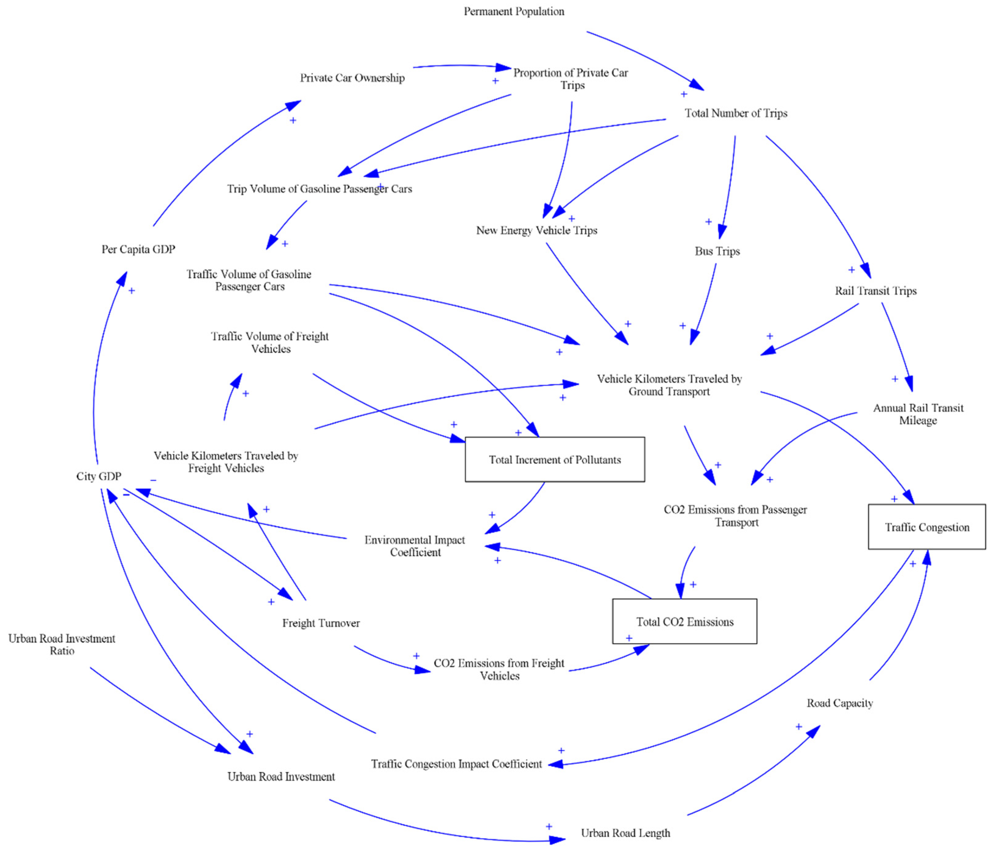
In system dynamics models, causal loop diagrams are crucial tools for visualizing causal relationships and feedback mechanisms within the system. In the causal loop diagram, the + symbol indicates a positive correlation (i.e., an increase in the source variable leads to an increase in the target variable); the − symbol indicates a negative correlation (i.e., an increase in the source variable leads to a decrease in the target variable). Based on an in-depth study of the interaction between Shanghai’s transportation system and its socio-economic and environmental subsystems, and considering the interaction mechanisms among the internal elements of these subsystems, a comprehensive causal loop diagram for the impact of urban traffic policies is constructed, as shown in Figure 2.
The main feedback loops in the model include the following:
  • Urban GDP → +Urban Road Investment → +Road Capacity → −Traffic Congestion → +Traffic Congestion Impact Coefficient → −Urban GDP Increment → +Urban GDP
This feedback loop indicates that as the urban GDP grows, investments in urban road infrastructure increase. The increase in road construction investment leads to an expansion in the total road mileage, enhancing road capacity, reducing traffic congestion, and further promoting urban GDP growth.
2.
Urban GDP → +Per Capita GDP → +Private Car Ownership → +Private Car Modal Share → +Private Car Travel Volume → +Private Car Traffic Volume → +Total Increment of Pollutants → +Environmental Impact Coefficient → +Urban GDP Increment → −Urban GDP
This feedback loop indicates that urban GDP growth promotes an increase in per capita GDP, which in turn leads to increased private car ownership. The higher car ownership rate results in a higher modal share for private cars and a corresponding increase in car travel volume, leading to higher energy consumption and more vehicle emissions, which negatively affect air quality and, consequently, urban economic development.
3.
Urban GDP → +Per Capita GDP → +Private Car Ownership → +Private Car Modal Share → +Private Car Travel Volume → +Private Car Traffic Volume → +Traffic Congestion → +Traffic Congestion Impact Coefficient → +Urban GDP Increment → −Urban GDP
This feedback loop indicates that urban GDP growth leads to an increase in per capita GDP, which encourages more private car ownership. The higher ownership rate increases the number of private cars on the road, exacerbating surface traffic congestion and ultimately hindering urban economic growth.
4.
Traffic Congestion → +Traffic Congestion Impact Coefficient → −Urban GDP Increment → +Urban GDP → +Urban Road Investment → +Road Capacity → −Traffic Congestion
This feedback loop indicates that traffic congestion negatively impacts urban economic growth, which in turn affects investments in road infrastructure, reducing road capacity and exacerbating traffic congestion.
5.
Traffic Congestion → +Traffic Congestion Impact Coefficient → −Urban GDP Increment → +Urban GDP → +Per Capita GDP → +Private Car Ownership → +Private Car Modal Share → +Gasoline Car Travel Volume → +Gasoline Car Traffic Volume → +Vehicle Kilometers Traveled by Ground Transport → +Traffic Congestion
This feedback loop indicates that traffic congestion reduces economic growth, which slows the increase in per capita GDP and private car ownership, ultimately decreasing the volume of car travel and reducing surface transport kilometers, which helps alleviate traffic congestion.
6.
Traffic Congestion → +Traffic Congestion Impact Coefficient → −Urban GDP Increment → +Urban GDP → +Freight Turnover → +Vehicle Kilometers Traveled by Freight Vehicles → +Vehicle Kilometers Traveled by Ground Transport → +Traffic Congestion
This feedback loop indicates that traffic congestion reduces urban GDP, which in turn reduces freight turnover and truck vehicle kilometers, thus easing surface transport congestion.
7.
Total Increment of Pollutants → +Environmental Impact Coefficient → −Urban GDP Increment → +Urban GDP → +Freight Turnover → +Vehicle Kilometers Traveled by Freight Vehicles → +CO2 Emissions from Freight Vehicles
This feedback loop indicates that increased emissions negatively impact urban GDP growth, which reduces freight turnover and truck vehicle kilometers, ultimately lowering pollution from trucks.
8.
Total Increment of Pollutants → +Environmental Impact Coefficient → −Urban GDP Increment → +Urban GDP → +Per Capita GDP → +Private Car Ownership → +Private Car Modal Share → +Gasoline Car Travel Volume → +Gasoline Car Traffic Volume → +Total Increment of Pollutants
This feedback loop indicates that increasing emissions hinder urban GDP growth, which slows the growth of per capita GDP and private car ownership, thereby reducing travel volumes and energy consumption, and ultimately lowering emissions.

3.1.2. System Flow Diagram and Model Structural Equations

  • Socio-Economic Subsystem
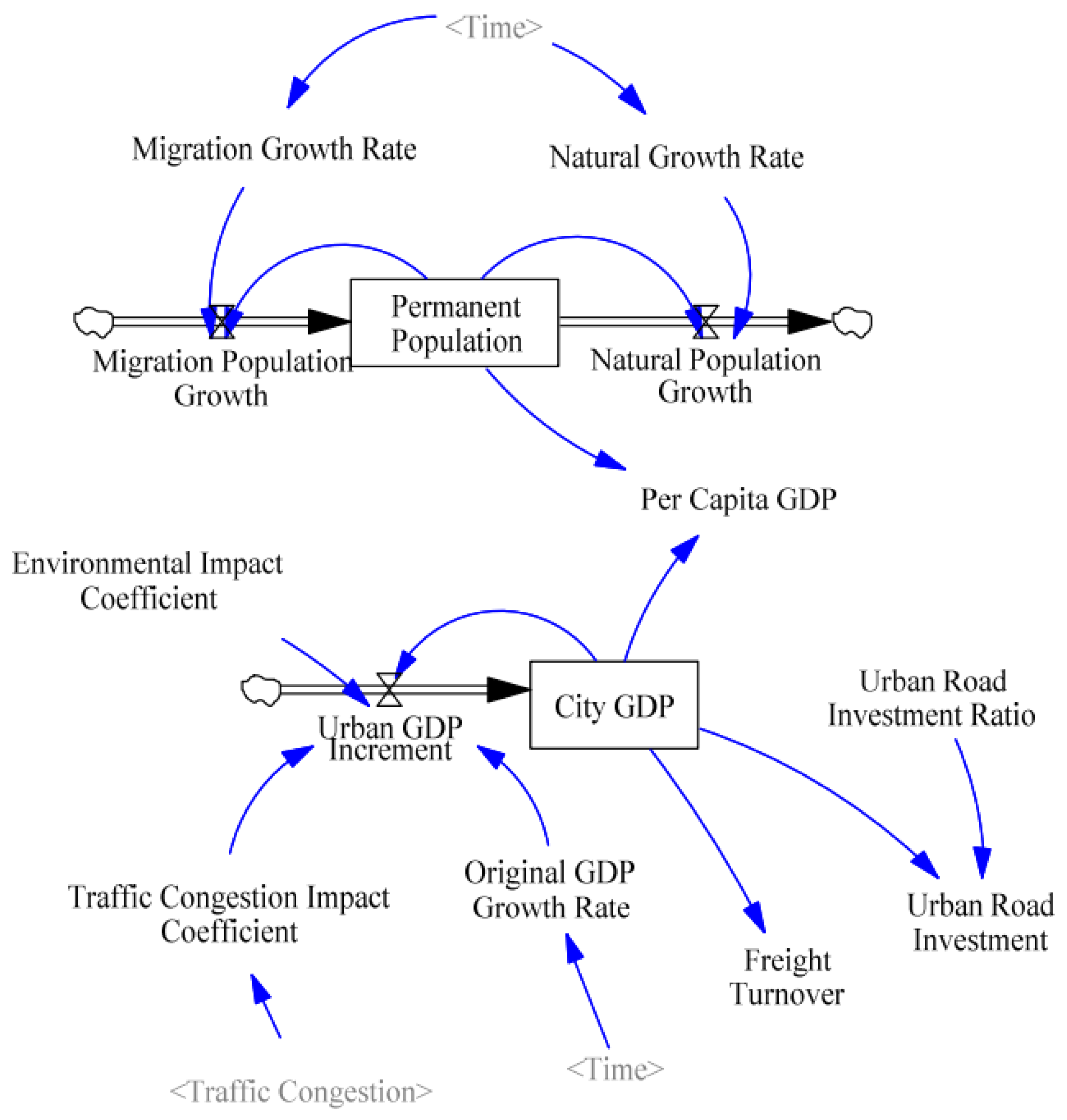
The socio-economic subsystem is a key subsystem for measuring the level of urban development. As the urban population continues to grow, the demand for transportation also gradually increases, leading to a rise in travel volume and passenger turnover. At the same time, the development of the urban economy also promotes urban transportation construction. Additionally, the socio-economic subsystem closely affects the traffic environment subsystem. Due to the increase in total travel volume, the demand for energy in transportation is continually expanding, which subsequently leads to corresponding pollutant emissions and carbon emissions. The flow diagram of the socio-economic subsystem is shown in Figure 3.
This subsystem has two stock variables: resident population and urban GDP. The rate variables include urban GDP increment, mechanical population growth, and natural population growth. Auxiliary variables include mechanical population growth rate, GDP growth rate, traffic congestion impact coefficient, and environmental pollution impact coefficient. The main structural equations are as follows:
T P t = T P t 1 + t 1 t ( N P I + M P I ) d t
N P I = T P t 1 × N P R t
M P I = T P t 1 × M P R t
where
  • T P t —Total population at time t
  • N P I t —Natural population increase at time t
  • M P I t —Mechanical population increase at time t
  • N P R t —Natural population growth rate at time t
  • M P R t —Mechanical population growth rate at time t.
Natural Population Increase is defined as the population flow resulting from the net effect of births minus deaths, capturing the natural growth or decline of the city’s population base. Mechanical Population Increase is defined as the net migration flow (inflow minus outflow) that captures non-natural population change, significantly influenced by economic and social factors.
G D P t = G D P t 1 + t 1 t G D P I d t
G D P I t = G D P t 1 × G D P I R t × ( 1 + C E R ) × ( 1 + C C R )
P C G t = G D P t ÷ T P t
where
  • G D P t —Gross Domestic Product at time t
  • G D P I t —Increment of GDP at time t
  • G D P I R t —Original GDP growth rate at time t
  • P C G t —Per capita GDP at time t
  • C C R ,     C E R —Traffic congestion impact coefficient, environmental pollution impact coefficient.
Traffic Congestion Impact Coefficient is an auxiliary coefficient that quantifies the negative feedback effect of traffic congestion levels on the city’s GDP growth rate. Environmental Pollution Impact Coefficient is an auxiliary coefficient that quantifies the negative feedback effect of ambient pollutant concentration (PE) on the city’s GDP growth rate.
2.
Urban Transportation Subsystem
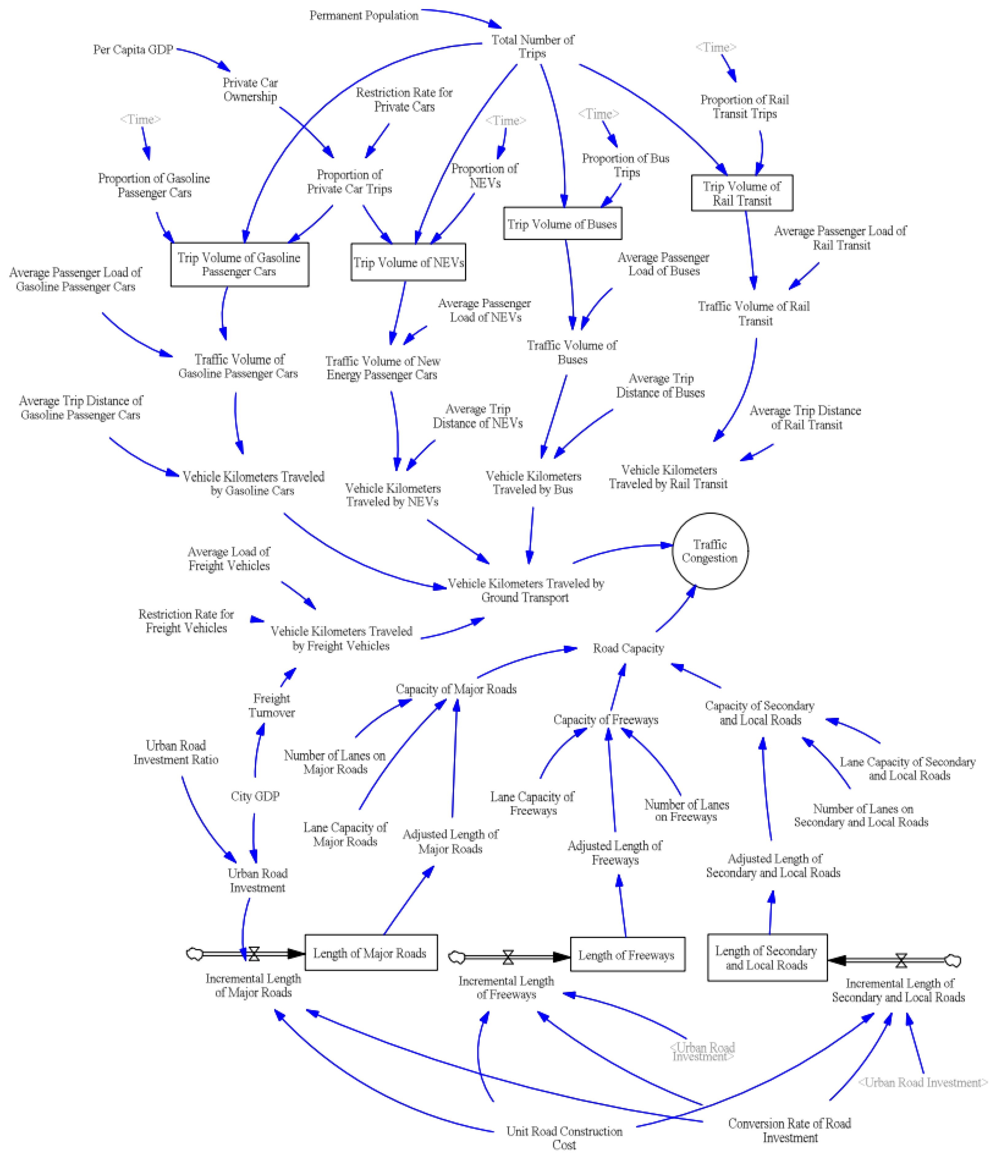
The urban transportation subsystem is a crucial component of the system, with close interrelationships and feedback mechanisms with other subsystems. In this subsystem, the focus is on studying the changing trends of urban traffic congestion and exploring the relationship between urban traffic and emissions. The changes in traffic congestion are not only determined by the travel volume of the urban population but are also related to urban transportation construction. By modeling and simulating the transportation subsystem, the complex interactions between these variables and other elements of the urban transportation system are explored. The modes of transportation included in the transportation subsystem are small cars, conventional ground public transport, trucks, and rail transit. The flow diagram of the urban transportation subsystem is shown in Figure 4.
This subsystem has two stock variables: the lengths of Major roads, Freeways, and secondary roads. The rate variables include the increment of the lengths of Major roads, Freeways, and secondary roads. Auxiliary variables include total travel volume, private car travel volume, bus travel volume, rail transit travel volume, private car traffic volume, bus traffic volume, vehicle miles traveled (VMT) for private cars, and VMT for buses. The main structural equations are as follows:
  • Urban Transportation Subsystem
G C T t = T N t × G C R t × G C T R t
N C T t = T N t × N C R t × N C T R t
B T t = T N t × B T R t
R T t = T N t × R T R t
where
  • T N t —Total number of trips at time t
  • G C T t , N C T t , B T t , R T t —Gasoline car trips at time t, new energy vehicle (NEV) trips at time t, Bus trips at time t, Rail transit trips at time t
  • G C R t , N C R t —Proportion of gasoline cars and NEVs at time t
  • G C T R t , N C T R t , B T R t , R T R t —Proportion of gasoline cars, NEVs, buses, and rail transit trips at time t
G C V t = G C T t N C × ( 1 P R A )
N C V t = N C T t N C × ( 1 P R A )
B V t = B T t N B
R V t = R T t N R
F V V t = F V D t F V S
where
  • G C V t , N C V t , B V t , R V t , F V V t —Gasoline car traffic volume at time t, NEV traffic volume at time t, bus traffic volume at time t, rail transit traffic volume at time t, and freight vehicles traffic volume at time t
  • N C , N B , N R —Average passenger capacity of cars, buses, and rail transit
  • P R A —Restriction policy
  • F V S —Average travel distance for freight vehicles
  • F V D t —Freight vehicle miles traveled (VMT) at time t
G C D t = G C V t × C S
N C D t = N C V t × C S
B D t = B V t × B S
R D t = R V t × R S
where
  • G C D t , N C D t , B D t , R D t —Gasoline car, NEV, bus, and rail transit vehicle distance traveled at time t
  • C S , B S , R S —Average travel distances for cars, buses, and rail transit
2.
Urban Road Supply Subsystem
F R L t = F R L t 1 + t 1 t F R L I d t
M R L t = M R L t 1 + t 1 t M R L I d t
S R L t = S R L t 1 + t 1 t S R L I d t
F R L I t 1 = 0.05 × R I t × R I C ÷ R P r i c e
M R L I t 1 = 0.15 × R I t × R I C ÷ R P r i c e
S R L I t 1 = 0.8 × R I t × R I C ÷ R P r i c e
R C = i = 1 3 C i × N i × R L i
where
  • F R L t , M R L t , S R L t —Freeway length at time t, major road length at time t, and secondary road and local road length at time t
  • F R L I , M R L I , S R L I —Increment in the freeway, major road, secondary, and local road length
  • R I t —Road infrastructure investment at time t
  • R I C —Road investment conversion rate
  • R P r i c e —Unit road construction cost
  • R C —Road capacity
  • C i —Lane capacity for road type i
  • N i —Number of lanes for road type i
  • R L i —Length of road type i
C I = 10,000 × V K T R C
where
  • V K T —Vehicle kilometers traveled by ground transport
The Congestion Index (CI) quantifies the saturation of the road system and serves as the primary output variable for evaluating policy impact on traffic conditions.
3.
Traffic Environment Subsystem
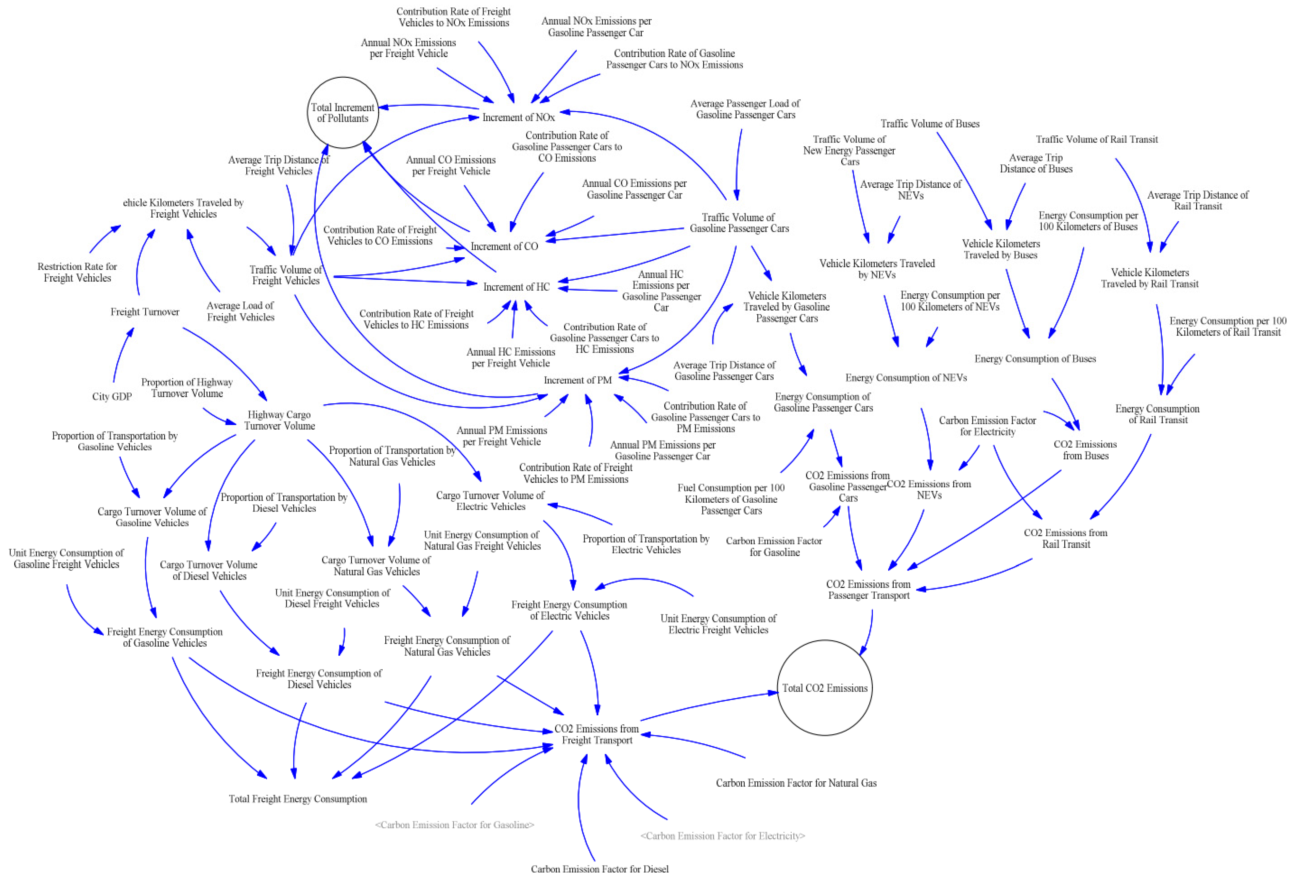
The Traffic Environment Subsystem is specifically designed to track not only greenhouse gas emissions (CO2) but also key local air pollutants, specifically NOx and PM, reflecting the study’s commitment to the dual environmental objective of GHG and local pollutant co-control. The flow diagram of the traffic environment subsystem is shown in Figure 5.
(1)
CO2 Emission
GCTEC t = GCD t × GCEC
N C T E C t = N C D t × N C E C
B T E C t = B D t × B E C
R T E C t = R D t × R E C
F V T E C t = F V D t × R E C
where
  • G C T E C t , N C T E C t , B T E C t , R T E C t , F V T E C t —Energy consumption of gasoline cars, NEVs, buses, rail transit, and freight vehicles at time t
  • G C E C , N C E C , B E C , R E C , F V E C —Energy consumption per 100 km for gasoline cars, NEVs, buses, rail transit, and freight vehicles
G C C E t = G C T E C t × G C E F
N C C E t = N C T E C t × E C E F
B C E t = B T E C t × E C E F
R C E t = R T E C t × E C E F
F V C E t = i F V T E C t × C E F i
T C E = G C C E + N C C E + B C E + R C E + F V C E
where
  • G C C E t , N C C E t , B C E t , R C E t , F V C E t CO2 emissions of gasoline cars, NEVs, buses, rail transit, and freight vehicles at time t
  • G C E F , D C E F , E C E F , N C E F —Carbon emission factors for gasoline, diesel, electricity, and natural gas
  • T C E —Total CO2 emissions
(2)
Pollutant Emissions
P I t = i G C W i × G C O i × G C V t + i F V W i × F V O i × F V V t
where
  • P I t —Annual pollutant increment
  • G C W i —Average annual emission of pollutant i per gasoline car
  • G C O i —Contribution rate of pollutant i from gasoline cars
  • F V W i —Average annual emission of pollutant i per freight vehicles
  • F V O i —Contribution rate of pollutant i from freight vehicles
Contribution Rate of Pollutant i from Gasoline Cars is the proportion of a specific pollutant i generated by the total volume of gasoline cars in the overall annual pollutant emissions (PI) from the traffic system. Contribution Rate of Pollutant i from Freight Vehicles is the proportion of a specific pollutant i generated by the total volume of freight vehicles in the overall annual pollutant emissions (PI) from the traffic system.
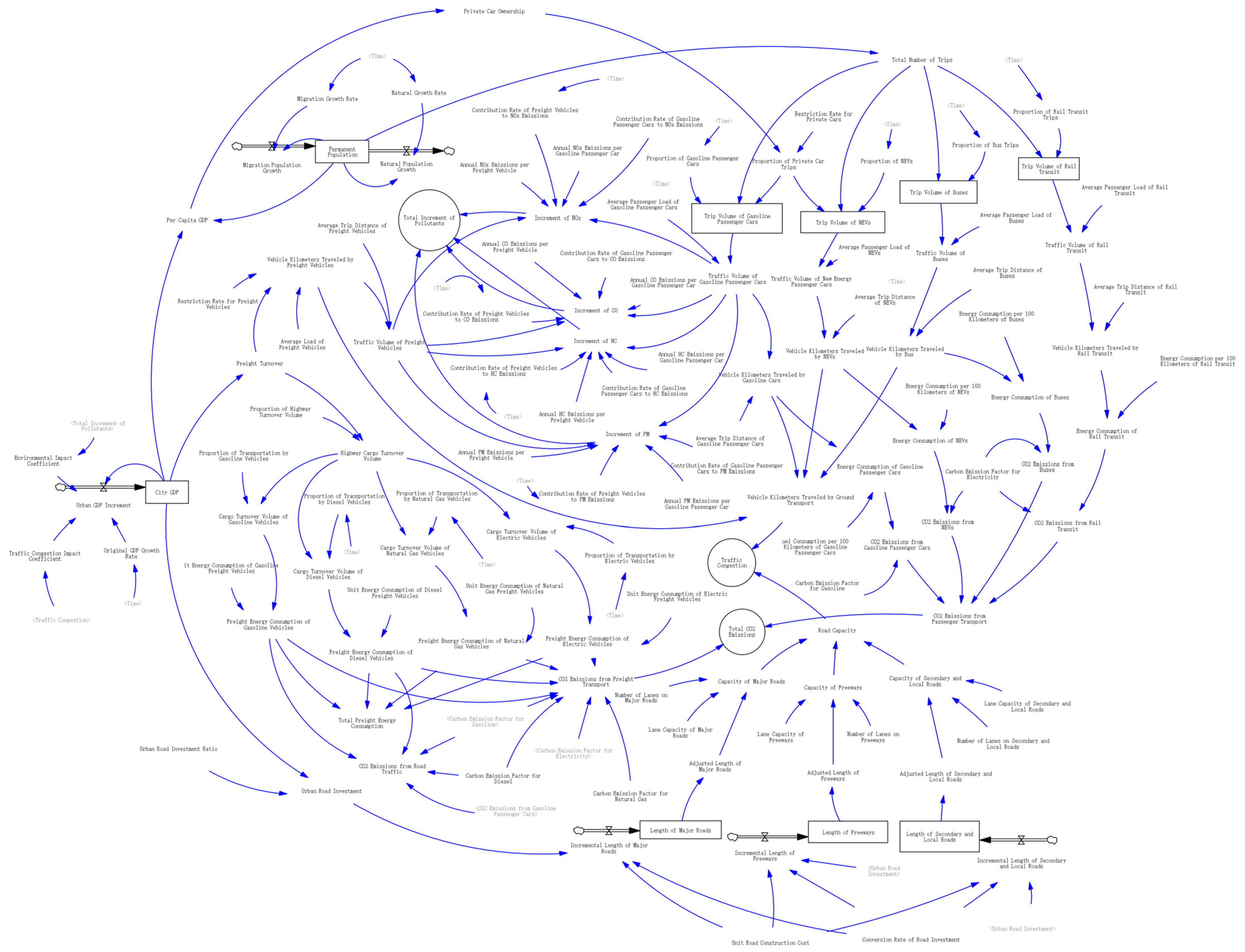
Based on the logical relationships among the internal variables of each subsystem and the quantitative analysis of the variables, a stock-and-flow diagram reflecting the feedback relationships among variables has been constructed based on the causal loop diagram. This is shown in Figure 6.

3.1.3. Parameter Design

Parameter estimation and validation are essential steps in system dynamics modeling, used to determine parameter values within the model and assess their accuracy and reliability. Utilizing data from the Shanghai Statistical Yearbook, relevant journal articles, and official websites, the initial values of stock variables and constant parameters were determined. The energy emission factors were derived from the “IPCC 2006 National Greenhouse Gas Inventory Guidelines” and its 2019 revision [32], while the 100 km energy consumption and average passenger capacity of various transportation modes were based on relevant studies. The specific values of carbon emission factors for energy are presented in Table 3.
The model’s partial parameters and initial values are shown in Table 4.
The proportion of trips made by cars (TN) is influenced by the total resident population (TP). Based on historical data, regression analysis using SPSS (Version 26, IBM Corp., Armonk, NY, USA) was performed, and the relationship between the two variables was obtained as follows:
T N = 2.029 × T P 1591.1
The fit test shows R2 = 0.978, which is close to 1, and a significance level of p = 0.00 < 0.05, indicating a strong linear relationship with statistical significance.
Similarly, freight turnover (FT) is linearly related to urban GDP (GDP). Based on historical data and regression analysis using SPSS, the relationship was obtained as:
F T = 0.697 × G D P + 3028.73
The fit test shows R2 = 0.929, and a significance level of p = 0.028 < 0.05, indicating a good fit and significant linear relationship between the variables.

3.1.4. Model Validation

  • Actual Consistency Test
The actual consistency test in system dynamics enhances the credibility of the model and research results by examining the error between the model’s simulation results and real-world conditions. This study selected Shanghai’s GDP, total resident population, and total travel volume as primary indicators for historical data validation. A comparison was made between historical data from 2010 to 2020 and the simulation values. Note that total travel volume data was only available from 2013 onward, thus the comparison for travel volume was limited to the years 2013 to 2020. Due to the impact of COVID-19 in 2020, there was a notable decrease in total travel volume, leading to significant discrepancies between actual and simulated values for that year. The maximum absolute error between the actual and simulated values of Shanghai’s GDP was 5.13%, which is also attributed to the unforeseen, external economic contraction during the COVID-19 period. The maximum absolute error between the actual and simulated values of resident population was 4.33%, and for total travel volume, it was 4.70%, all of which are within acceptable ranges. Excluding the impact of the pandemic in 2020, the simulation results showed a good fit with the historical data. Overall, the relative errors for the main indicators remained below 6%, indicating that the system dynamics model effectively reflects actual conditions and meets the simulation analysis requirements. The actual and simulated values of Shanghai’s GDP are presented in Table 5.
The actual and simulated values of the total resident population are shown in Table 6.
The actual and simulated values of total travel volume are shown in Table 7.
The validation process spanning 2010–2020 served primarily for parameter calibration and demonstration of historical fit. No separate hold-out period was utilized for out-of-sample testing, as the core objective of this SD model is long-term policy analysis and comparison of relative effectiveness, rather than short-term forecasting. Regarding the 2020 data point, which is acknowledged as a significant outlier, the core structural parameters of the model were predominantly calibrated using the stable data period (2010–2019).
2.
Extreme Condition Test
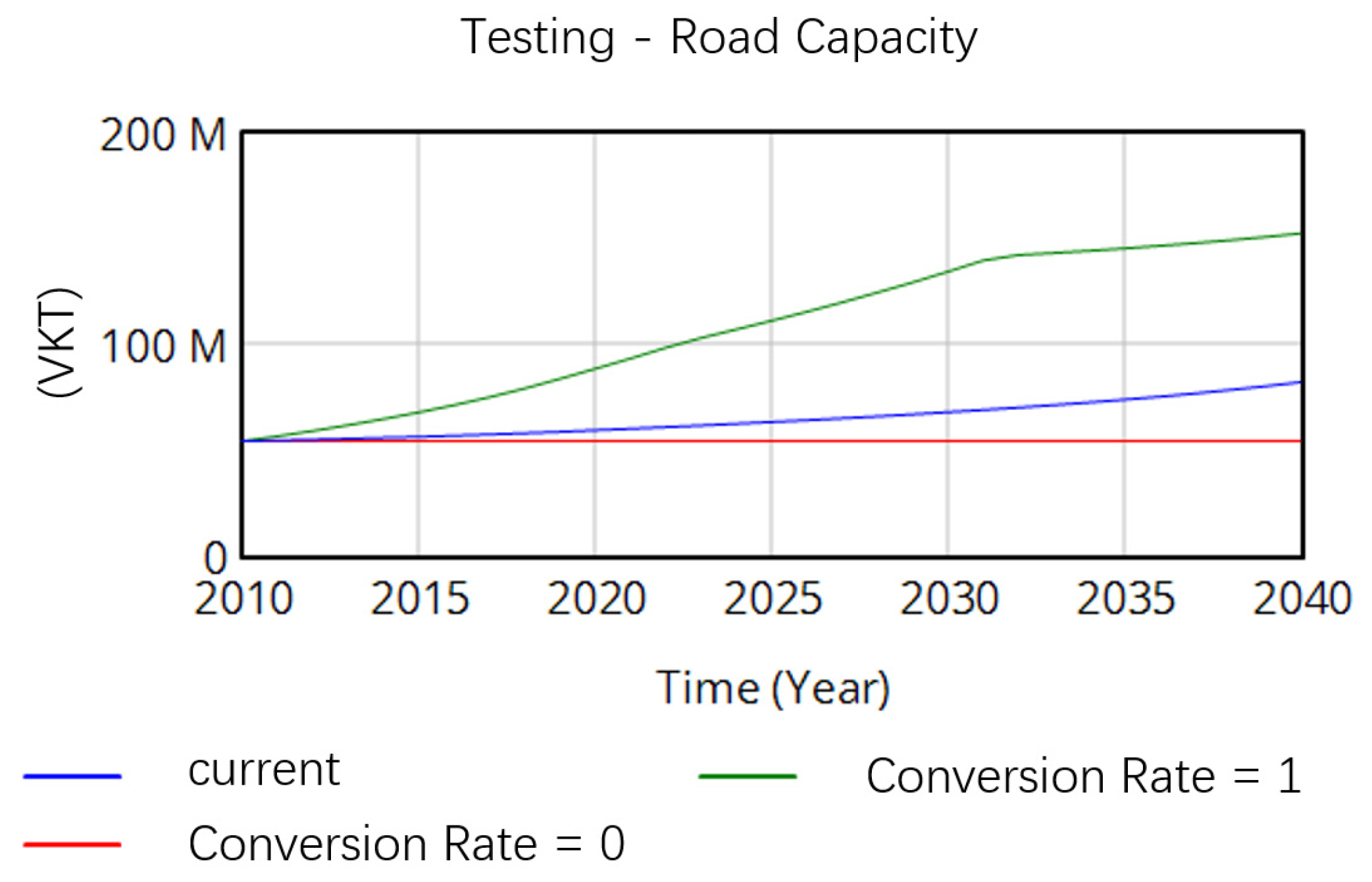
When using system dynamics models to simulate complex systems, extreme condition testing is crucial. This test helps ensure that the model maintains its stability and predictive accuracy in the face of unusual circumstances. Extreme condition testing involves sensitivity analysis of system parameters and boundary conditions. By simulating extreme values for parameters, the model’s performance under different extreme scenarios is evaluated to determine its validity in such conditions. Taking road capacity as an example, the road investment conversion rate is set to 0 and 1, respectively, and compared with the baseline scenario (road investment conversion rate of 0.15). The results are shown in Figure 7.
The figure indicates that when the road investment conversion rate is set to its extreme values of 0 and 1, the road capacity reaches its maximum and minimum values, respectively. When the conversion rate is 0, the increase in road length is 0, and the road capacity remains unchanged; when the conversion rate is 1, the road length significantly increases, but due to a set limit on road length in the model, the rate of increase in road capacity first accelerates and then slows. The corresponding output curves of the model are shown. Comparing the actual situation with the simulation results, the trends align with real-world conditions. Therefore, the model demonstrates reliability and accuracy.
3.
Sensitivity testing
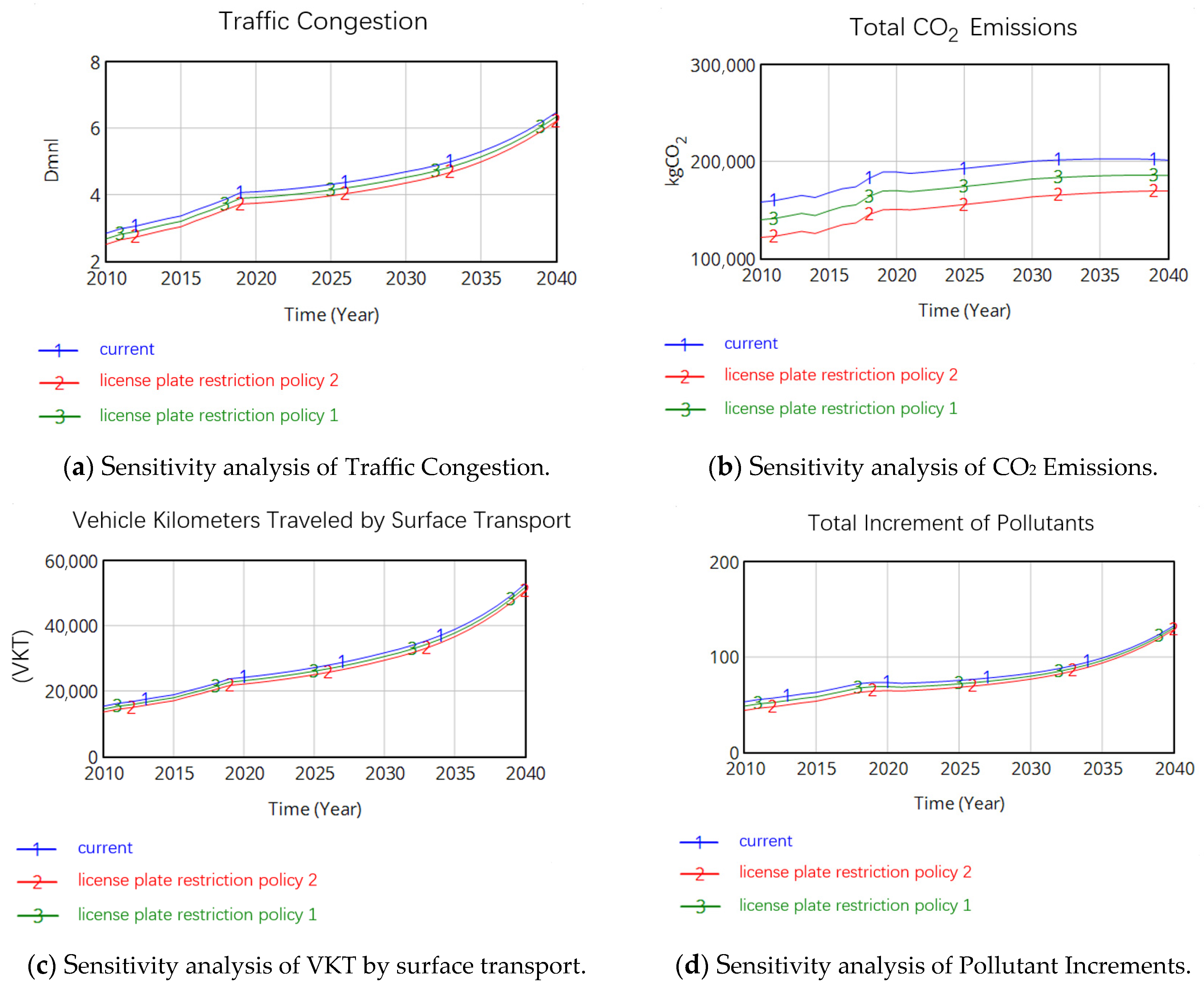
Sensitivity testing assesses the model’s responsiveness to changes in parameters. In conducting sensitivity tests in system dynamics, a series of parameter values must be set, monitoring how the model output varies with changes in specific parameters. If the model output exhibits significant changes with minor parameter adjustments, this indicates a degree of sensitivity to those parameters. This study observed the model’s sensitivity by varying values for different traffic restriction policies. Under Traffic Restriction Policy 1, the car restriction rate is set at 0.15, indicating that 15% of cars are restricted from traveling; under Traffic Restriction Policy 2, the restriction rate is set at 0.3, meaning 30% of cars are restricted. Simulations were conducted under both levels of restrictions to observe changes in traffic congestion, CO2 emissions, vehicle kilometers traveled, and NOx emissions. The simulation results are presented in Figure 8a–d.
Sensitivity testing confirmed that the inclusion or exclusion of the 2020 data point did not fundamentally alter the stability of the structural parameters nor the relative ranking and effectiveness of the policy scenarios presented in the Section 4. By comparing the changes in indicators in Figure 8a–d, it can be seen that as the car restriction rate increases, the travel volume of cars decreases, corresponding to reductions in traffic congestion, CO2 emissions, vehicle kilometers traveled, and pollutant emissions.

3.2. TOPSIS Model Construction

TOPSIS (Technique for Order of Preference by Similarity to Ideal Solution) is a widely used multi-criteria decision-making method that evaluates and ranks alternatives based on their proximity to an ideal solution. The core concept of TOPSIS is to assess the performance of each alternative by calculating its distance to the ideal solution, thereby enabling policymakers to rank and select policies based on their effectiveness. In this study, the TOPSIS method is applied to quantitatively evaluate traffic congestion mitigation and emission reduction policies, following the simulation and optimization of their effects using a system dynamics model. By considering three evaluation criteria—traffic congestion, carbon emissions, and pollutant emissions—this study conducts a quantitative analysis of policy implementation. Traffic congestion is a negative criterion where higher values indicate more severe traffic issues, and both carbon and pollutant emissions are also negative criteria, with higher emissions reflecting greater adverse environmental impacts.
To ensure comparability across criteria with differing units and magnitudes, range normalization is applied to standardize the data, ensuring fairness in the results. The detailed steps of the TOPSIS calculation are as follows:
  • Constructing the Decision Matrix
The decision matrix is established by organizing the scores of various policies across all criteria. Assuming there are six policies and three evaluation criteria, the decision matrix can be expressed as follows:
P 1     X 11     X 12     X 13 P 2     X 21     X 22     X 23                                           P 6     X 61     X 62     X 63
where, P i represents the i-th policy, and X i j is the score of the i-th policy on the j-th criterion.
2.
Standardizing the Decision Matrix
Since the evaluation criteria have different units and scales, the data are standardized using range normalization to eliminate the influence of dimensions and ensure comparability among criteria. For negative criteria, the normalization formula is as follows:
X i j = X i j X min j X max j X min j  
where X i j is the original value of policy i on criterion j, and X m a x   j and X min j are the maximum and minimum values of criterion j, respectively.
3.
Calculating the Weighted Normalized Matrix
To reflect the relative importance of each criterion, the standardized data are weighted, resulting in the weighted normalized matrix:
V i j = w i j × X i j
where w i j is the weight of criterion j, and V i j is the weighted normalized score of policy i on criterion j.
4.
Identifying the Ideal and Negative Ideal Solutions
The ideal solution V + and negative ideal solution V represent the best and worst scores across all policies for each criterion, respectively:
V + = m a x 1 j m v i j j = 1,2 , 3 = v 1 + , v 2 + , v 3 +
V = m i n 1 j m v i j j = 1,2 , 3 = v 1 , v 2 , v 3
where v 1 + , v 2 + , v 3 + are the ideal values for each criterion, and v 1 , v 2 , v 3 are the corresponding negative ideal values.
5.
Calculating the Distances to the Ideal and Negative Ideal Solutions
The Euclidean distances between each alternative and the ideal ( D i + ) and negative ideal ( D i ) solutions are calculated as follows:
D i + = j = 1 n ( V i j V j + ) 2
D i = j = 1 n ( V i j V j ) 2
where V j + and V j are the ideal and negative ideal values for criterion j, respectively.
6.
Computing the Closeness Coefficient
The closeness coefficient quantifies the proximity of each alternative to the ideal solution. It is calculated using the following formula:
C i = D i D i + + D i
where a larger C i value indicates that the policy is closer to the ideal solution.

4. Results and Discussion

For accurate interpretation of the long-term simulation results, it is necessary to clarify the criteria for policy success. The simulated curves for all policy scenarios show that while the absolute values of congestion, CO2, and pollutants may trend gradually upward in the long term, this is not indicative of policy failure. This upward movement is a direct reflection of the overwhelming, continuous growth pressure exerted by exogenous socio-economic drivers (e.g., population and economic activity) as modeled in the Baseline Scenario. The true measure of policy success in this dynamic system is not a permanent absolute decline, but the success in maintaining a significant and sustained deviation (i.e., control) compared to the No-Policy Baseline Scenario across the entire planning horizon. This sustained relative gap unequivocally demonstrates the policy’s long-term cumulative mitigation value and control over the acceleration of negative externalities.

4.1. Simulation and Optimization of Urban Traffic Congestion Mitigation and Emission Reduction Policies

Through the adjustment of relevant variables in the established model, this study constructed multiple simulation scenarios under various policy combinations to simulate the effects of different policy scenarios implemented in Shanghai from 2010 to 2040. The research aims to provide references for alleviating traffic congestion and reducing emissions in Shanghai, while offering theoretical support and scientific basis for the formulation of effective policy solutions. The model scenarios are based on an in-depth analysis of the relationship between urban traffic congestion and carbon emissions, as well as case studies, to achieve more precise result predictions and effective policy development. This study considers changes in carbon emissions under different levels of traffic congestion and explores the impacts of various governance strategies on traffic congestion and emissions. Utilizing historical data from 2010 to 2020 as a baseline, the trends of Shanghai’s economic growth, population changes, urban passenger and freight transport structure, and transportation supply levels are assumed to continue in the future research period, indicating that, under the existing policy framework, the road traffic patterns in Shanghai will persist. This baseline scenario will provide a reference for comparison with other scenario models. Additionally, considering Shanghai’s future policy needs, this study has established five policy scenarios, including the license plate restriction policy, road investment policy, technology improvement policy, carpooling policy, and new energy vehicle promotion policy.
  • Simulation Analysis of New Energy Vehicle Promotion Policy
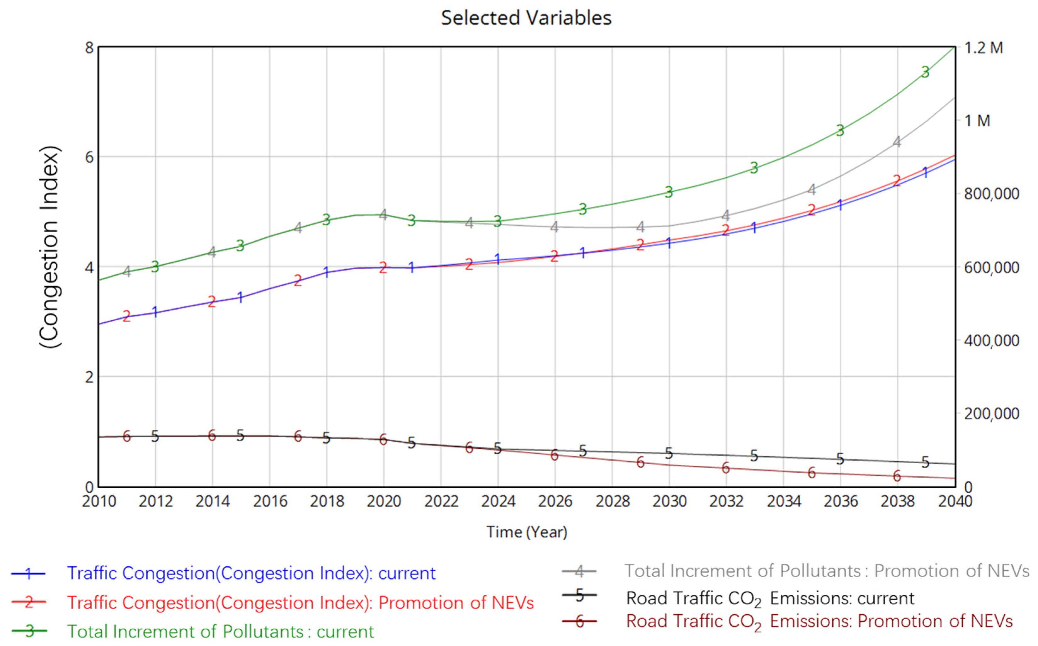
The promotion of new energy vehicles can reduce the usage of traditional fuel vehicles, thereby impacting traffic carbon emissions and air quality, as well as influencing the energy structure. This paper simulates the promotion policy by adjusting the ratio of gasoline vehicles to new energy vehicles, specifically increasing the proportion of new energy vehicles by 30% while decreasing the proportion of gasoline vehicles by 30%. The scenario’s 30% increase in NEV adoption preference is justified by both current market performance and national policy mandates. This target is highly feasible and conservative, as the NEV new car penetration rate in China already reached 30.8% in the first eleven months of 2023, according to the 2023 Annual Evaluation Report by China SAE (SAE-China, 2023 [33]). Given that the annual sales flow surpasses this level, 30% is affirmed as a reliable mid-term target for the total vehicle stock. Furthermore, national documents (e.g., the NEV Technology Roadmap) mandate a new car penetration rate of over 50% by 2035. Consequently, this 30% increment is designed to simulate a high-intensity, accelerated policy intervention scenario—reflecting the robust push required for pioneering cities like Shanghai to meet these national goals—allowing the model to test the maximum potential environmental benefit under aggressive electrification. The simulation results of the new energy vehicle promotion policy are shown in Figure 9.
Conflict Between Congestion Mitigation and Emission Reduction: In the early stages of implementing the new energy vehicle promotion policy, significant reductions in traffic carbon emissions and pollutants can be observed. However, the popularity of new energy vehicles may attract more consumers to purchase vehicles. As the penetration rate of new energy vehicles increases, this may ultimately lead to an increase in the total number of motor vehicles, thereby exacerbating traffic congestion. On the other hand, the demand for charging new energy vehicles may complicate urban traffic, particularly in cases where charging infrastructure is poorly laid out, potentially leading to increased congestion.
Therefore, achieving a complete coupling between congestion mitigation and emission reduction through this policy is challenging. It is necessary to comprehensively consider various factors and their impacts over time, adopting integrated measures to balance the relationship between the two objectives, ensuring the long-term benefits of the policy and the sustainable development of traffic.
2.
Simulation Analysis of License Plate Restriction Policy
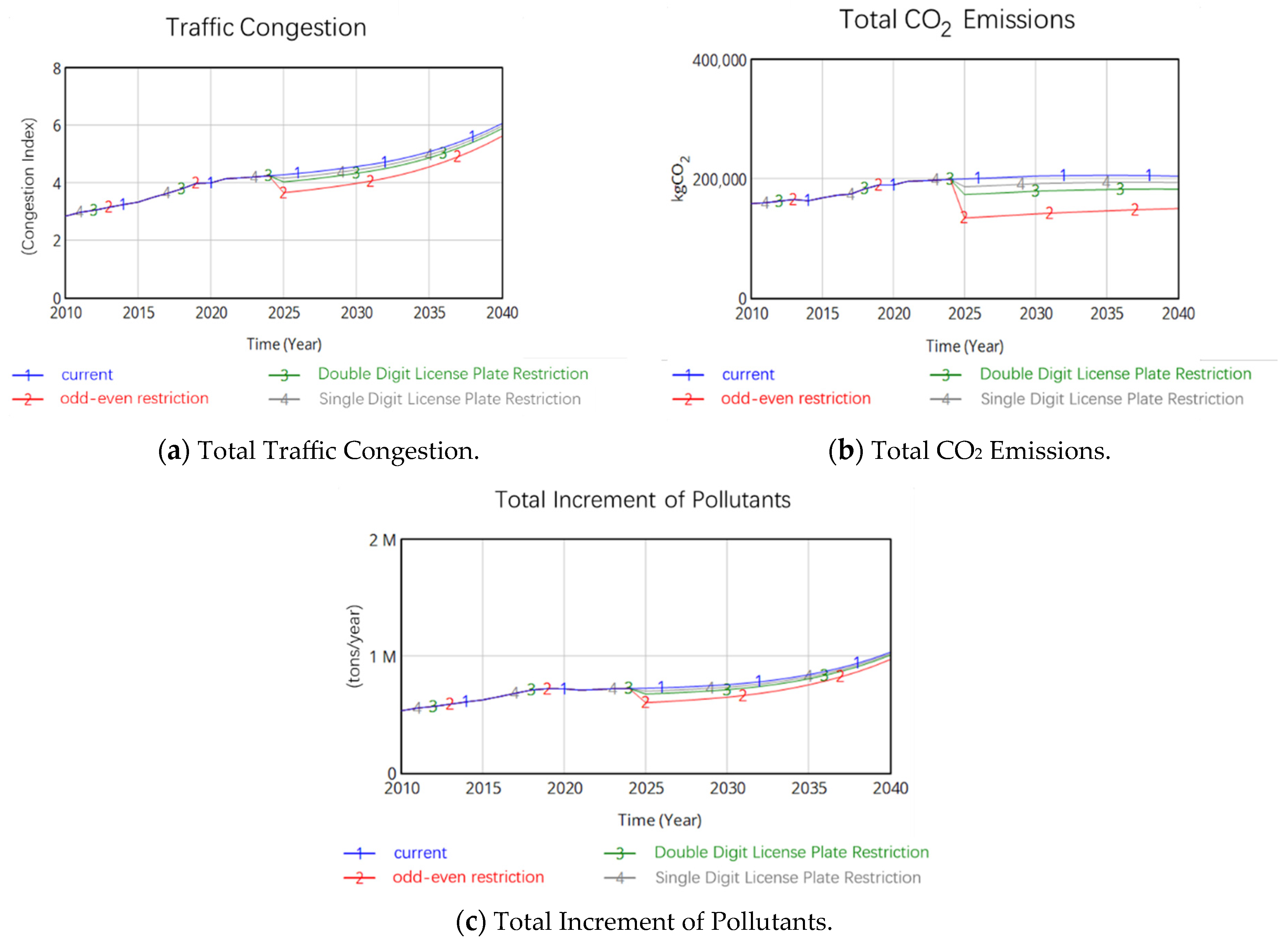
The license plate restriction policy is a common traffic control measure that can help disperse traffic flow, alleviate congestion, and reduce vehicle emissions. Currently, in Shanghai, only small passenger cars with license plates from other provinces are subject to restrictions, which are categorized into elevated (expressway) restrictions and inner ring ground restrictions. Elevated (expressway) restrictions are in effect from Monday to Friday, 07:00 to 20:00 (a total of 13 h), while inner ring ground restrictions apply from Monday to Friday, 07:00 to 09:00 and 17:00 to 19:00 (a total of 4 h). There are no restrictions on weekends and public holidays. This study considers incorporating the license plate restriction policy into the model to observe and analyze the resulting impacts. The small car restriction policy is categorized into unrestricted, single-digit license plate restriction, double-digit license plate restriction, and odd-even restriction, with the corresponding reductions in the number of car trips set at 10%, 20%, and 50%, respectively. The simulation results of the license plate restriction policy are shown in Figure 10.
Short-term Effects and Long-term Potential of the Policy: The license plate restriction policy can effectively reduce traffic flow and pollutant emissions. As the intensity of the restriction policy increases, traffic flow decreases significantly, leading to substantial reductions in traffic congestion and emissions, particularly with the odd-even restriction showing the most pronounced effects. In the short term, this policy serves as an effective means of controlling traffic volume, but in the long term, the trend of the curves indicates a gradual return to previous levels. This suggests that the effectiveness of the policy may be undermined by evasive behaviors, with traffic demand potentially rebounding. For example, an increase in vehicle ownership could lead to a resurgence of congestion and emissions. Therefore, the restriction policy needs to be integrated with long-term traffic demand management strategies, such as promoting public transportation and non-motorized travel, to ensure that the restriction policy aligns with improvements in public transport supply, guiding residents towards choosing public transport or non-motorized travel to achieve long-term reductions in traffic congestion.
3.
Simulation Analysis of Road Investment Policy
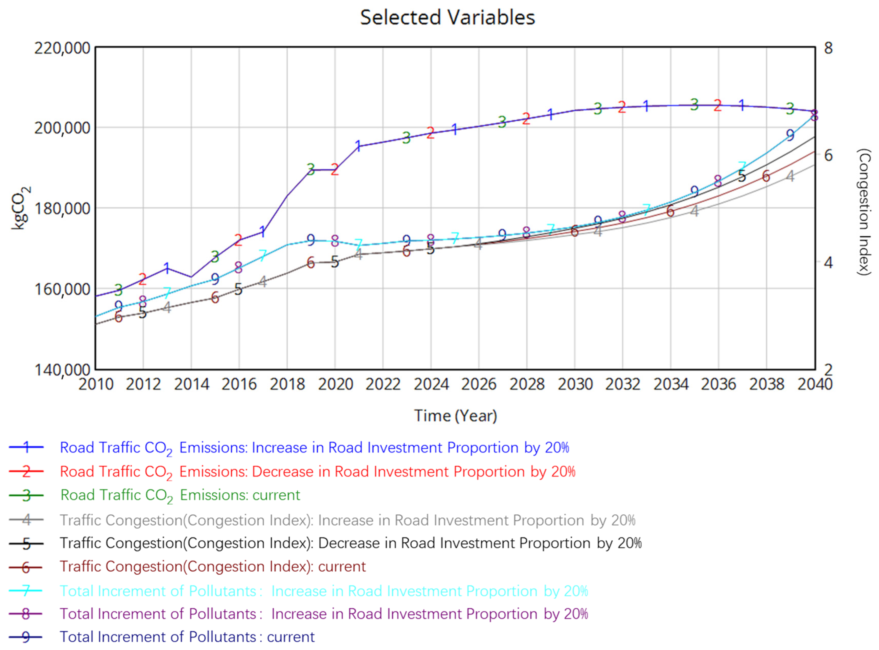
Road investment closely affects the supply of urban roads, consequently impacting traffic congestion, carbon emissions, and roadway pollutants. This study alters the proportion of road investment to change urban road investments, categorizing the road investment policy into two scenarios: increasing urban road investment by 20% and decreasing it by 20%. The Urban Road Increment is set at 20% to simulate a major, high-investment ceiling scenario within the model. The parameter setting is based not on statistical projection, but on the necessity of policy goals and the constraint of urban space. Firstly, this high-effort intensity aligns with the explicit policy mandate in the Shanghai Master Plan (2017–2035) for the “continual optimization of the road network structure and increasing road network density.” Secondly, given the scarcity of space in the core urban area of a megacity, any significant expansion requires extremely high construction costs. The simulation results of the road investment policy are illustrated in Figure 11.
Induced Demand: The results indicate that while road investment policies can temporarily alleviate traffic congestion, their impact on carbon and pollutant emissions is relatively minor. This is because the increase in road supply may induce more traffic demand, resulting in an increase in traffic volume over the long term, which can offset the emission reductions achieved through congestion mitigation, leading to no significant decrease in carbon and pollutant emissions. Therefore, this policy should be coordinated with demand management measures, such as restricting the use of cars or increasing public transport supply, to achieve more comprehensive emission reduction goals.
4.
Simulation Analysis of Ridesplitting Policy
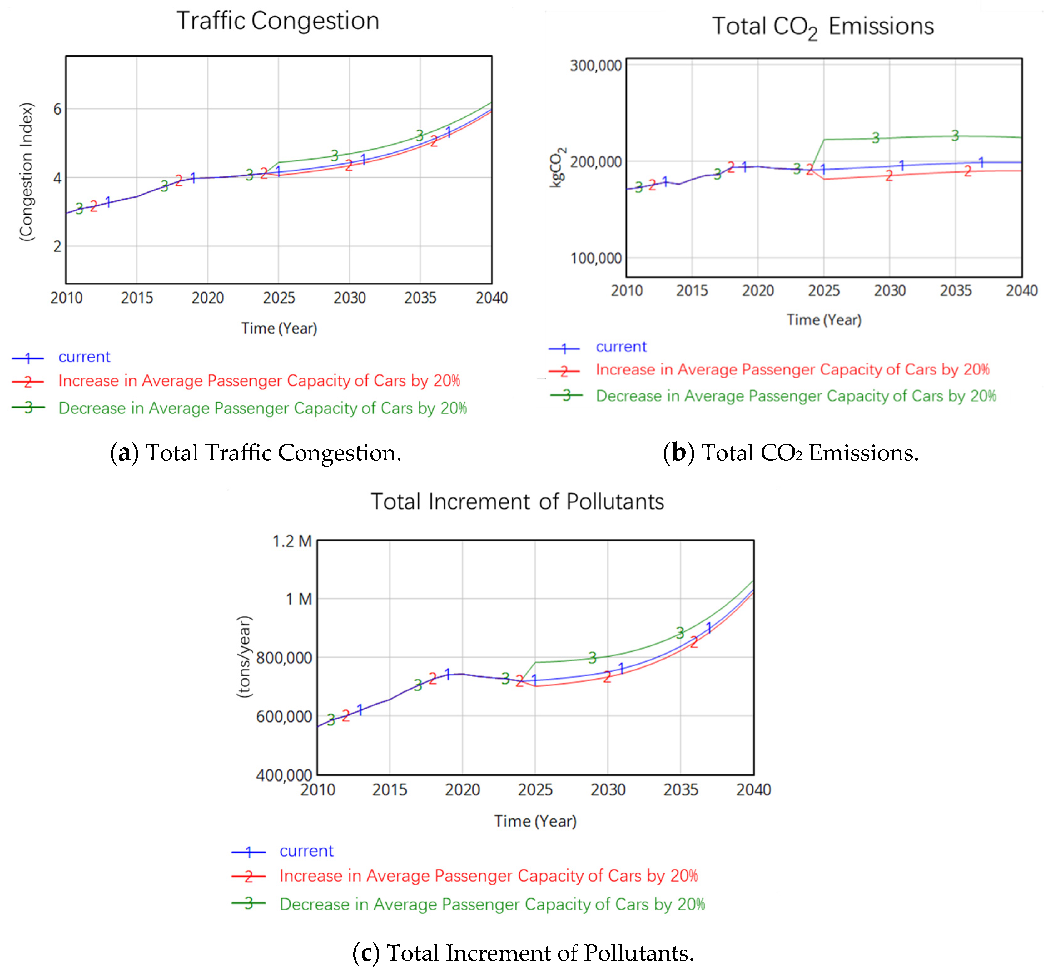
Ridesplitting allows more individuals to share a vehicle rather than requiring one vehicle per traveler for each trip, thus enhancing the capacity of transportation tools and reducing traffic volume on the roads. This study simulates the carpooling policy by changing the average passenger capacity of cars, categorizing the policy into two scenarios: increasing the average passenger capacity of cars by 20% and decreasing it by 20%. The ±20% change in the Average Occupancy Rate is chosen to reflect the maximum feasible impact of policy incentives (Policy Ceiling Simulation, +20%) and to serve as a sensitivity test floor (−20%) for assessing the full efficacy range of this demand-side management tool. The simulation results of the carpooling policy are shown in Figure 12.
Potential for Enhanced Travel Efficiency: The simulation results indicate that the carpooling policy effectively reduces the number of vehicles on the road, thereby decreasing traffic congestion and carbon emissions by increasing the average passenger capacity of cars. However, the data also show that while increasing passenger capacity, carpooling may lead to longer travel distances due to detours, which can offset some of the emission reduction effects. The positive impacts of carpooling coexist with potential negative effects, necessitating a comprehensive consideration of its overall influence on traffic flow.
Asymmetry Effects: The policy’s positive and negative impacts exhibit asymmetry. While increasing the average passenger capacity of cars should theoretically reduce traffic volume and carbon emissions, in practice, due to Shanghai’s high population and vehicle density, the actual reduction in the number of vehicles may fall short of expectations. Conversely, decreasing average passenger capacity would directly lead to an increase in vehicle numbers, and any additional vehicles could significantly exacerbate congestion, a negative effect that is notably evident in the data.
5.
Simulation Analysis of Technology Improvement Policy
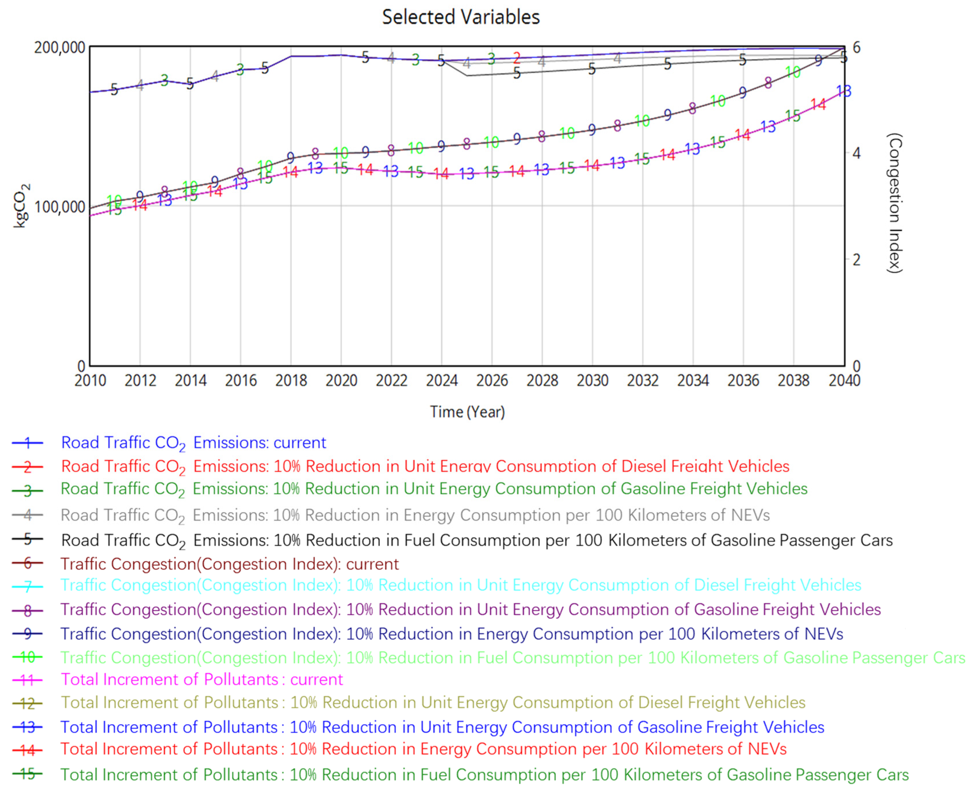
Advancements in vehicle engine technology will help improve the energy efficiency of vehicles, thereby reducing energy consumption and carbon emissions associated with vehicle operation. This study simulates the technology improvement policy by altering the 100 km fuel consumption of gasoline cars, categorizing the policy into four scenarios: decreasing the 100 km fuel consumption of gasoline cars and new energy vehicles by 10%, and reducing the unit energy consumption of diesel and gasoline freight vehicles by 10%. The simulation results of the technology improvement policy are illustrated in Figure 13.
The results show that the policy has a significant impact on carbon emissions, with gasoline cars being the most affected due to fuel consumption directly influencing carbon emissions. However, as new energy vehicles become more widespread, the proportion of gasoline cars decreases, and the policy’s emission reduction capability weakens, leading to a rebound in carbon emissions later in the policy implementation. Simultaneously, the increase in the traffic volume of new energy vehicles strengthens the impact of reduced energy consumption per 100 km on carbon emissions. In contrast, the relatively lower number of freight vehicles means that reductions in their unit energy consumption have a limited impact on overall carbon emissions. Therefore, relying solely on technological improvements may not ensure sustained emission reduction outcomes. A comprehensive consideration of the characteristics of different types of vehicles and the synergistic effects of policies is essential to achieve long-term emission reduction targets.

4.2. Evaluation of Traffic Congestion Mitigation and Emission Reduction Policies Based on the TOPSIS Model

Using the simulation data from 2040 and the TOPSIS method, the closeness coefficients of various policies were calculated for evaluation. The evaluated policies include promotion of new energy vehicles (Y1), restriction of two license plate numbers (Y2), road investment (Y3), carpooling (Y4), reduction of fuel consumption for private vehicles (Y5), and reduction of energy consumption for new energy vehicles (Y6). The evaluation criteria are traffic congestion (C1), carbon emissions (C2), and pollutant emissions (C3). The raw data were processed using the range normalization method, compressing the values of each indicator into the [0, 1] range. The normalized indicator matrix is shown in Table 8.
After normalization, the entropy weight method was used to determine the weights of each evaluation criterion, which were 0.309 for traffic congestion, 0.356 for carbon emissions, and 0.335 for pollutant emissions. The normalized indicator matrix was then weighted to obtain the weighted decision matrix, as shown in Table 9.
Based on the weighted decision matrix, the Euclidean distances of each policy from the ideal solution and the negative ideal solution were calculated. Subsequently, the closeness coefficients, which represent the relative proximity of each policy to the ideal solution, were derived. The closeness coefficients range from 0 to 1, with larger values indicating better overall performance. The closeness coefficients are summarized in Table 10.
Based on the ranking of closeness coefficients in descending order, the priority sequence of the evaluated policies is Y2 > Y4 > Y1 > Y3 > Y5 > Y6. The results show that:
Restriction of two license plate numbers (Y2) performs the best among all policies, demonstrating the direct effectiveness of mandatory traffic control measures in mitigating traffic congestion and reducing emissions.
Carpooling (Y4), though less impactful in the short term compared to restriction policies, has significant long-term potential by optimizing traffic flow and reducing single-vehicle trips, thus improving road efficiency.
The promotion of new energy vehicles (Y1) has a long-term positive impact on emission reduction. However, its direct effect on alleviating traffic congestion is limited, as widespread adoption takes time.
Road investment (Y3) improves traffic capacity in the short term but may lead to induced demand, resulting in increased traffic flow and reduced long-term benefits.
Reduction of fuel consumption for private vehicles (Y5) and reduction of energy consumption for new energy vehicles (Y6) focus primarily on improving vehicle efficiency, with limited impact on overall traffic flow. Hence, they rank lower in this evaluation.
In conclusion, restriction policies have the most immediate and significant impact on traffic flow and emission reduction. Carpooling policies, while slower in achieving results, offer substantial long-term benefits. Meanwhile, policies such as new energy vehicle promotion and road investment have relatively limited effects on traffic mitigation and are subject to time-dependent factors. Technical optimization policies, although environmentally beneficial, contribute little to traffic congestion mitigation in the short term. These differences in policy effectiveness highlight their varied focuses on traffic management, emission control, and behavioral changes.

5. Conclusions and Implications

This study integrates a system dynamics approach with the TOPSIS evaluation framework to construct a comprehensive analytical model, thoroughly exploring the dynamic coupling relationships among urban traffic congestion, carbon emissions, and mitigation policies in megacities. Using the Shanghai traffic system as a case study, the analysis investigates the mechanisms of different governance strategies in both the short and long term. Furthermore, the study employs the TOPSIS method to quantitatively evaluate the multidimensional effectiveness of various policies, leading to the following conclusions:
Non-coordinated coupling of traffic congestion, carbon emissions, and environmental pollution: Single policies may alleviate one indicator while exacerbating the negative effects on other indicators, leading to heterogeneous governance outcomes. For example, the promotion of new energy vehicles did not significantly alleviate traffic congestion in the short term, but instead led to a 0.3152% increase in congestion. However, the policy showed significant reductions in carbon emissions and pollutant emissions, with reductions of 4.3451% and 3.9119%, respectively. This indicates that, while the promotion of new energy vehicles can effectively reduce carbon emissions and pollutants, its impact on traffic congestion is limited in the short term. The “congestion-emissions-pollution” negative feedback loop further highlights the complexity of urban traffic governance, where a single policy is unlikely to simultaneously optimize traffic congestion, carbon emissions, and pollution. Therefore, multi-objective coordinated governance requires a systemic perspective that considers the dynamic interactions and long-term impacts of various factors from the policy design stage.
Short-term and long-term policy effects: The restriction policy significantly reduced traffic congestion, carbon emissions, and pollutant emissions in the short term. Specifically, in 2030, it reduced congestion, carbon emissions, and pollutant emissions by 4.7288%, 12.037%, and 5.6614%, respectively. However, by 2040, with the prolonged implementation of the policy, its effects showed a diminishing trend, with reductions in congestion, carbon emissions, and pollutant emissions decreasing to 2.7205%, 10.3788%, and 2.4738%, respectively. This result suggests that the restriction policy can rapidly ease traffic pressure and significantly reduce emissions in the short term, but its long-term effectiveness diminishes due to the adaptability of the transportation system and other external factors. Thus, the effectiveness of a single policy may decline over time, and it is necessary to combine other policy measures to ensure sustained and effective traffic governance and emission reduction. Additionally, the TOPSIS results indicate that the “two-license-plate restriction” policy achieves the highest overall governance effectiveness, with a composite effectiveness score of 0.68. In contrast, the “promotion of new energy vehicles” policy contributes significantly to long-term emission reductions but has a lower composite score of 0.5. This result underscores the complementarity of different policies within the governance framework and emphasizes the importance of policy synergy.
In summary, this study provides three core, actionable policy references derived from the integrated SD-TOPSIS framework, offering a quantifiable basis for megacity governance. This framework equips municipal authorities with a systematic tool to objectively rank and select the optimal policy portfolio that balances economic, traffic, and environmental goals. The practical contributions are:
1. Strategic Policy Differentiation is Mandatory: Policy-makers must clearly separate environmental goals from congestion management. Our data confirms that NEV promotion acts primarily as an effective environmental tool (4.3451% CO2 reduction) but is ineffective for congestion relief, as it slightly exacerbates traffic volume (0.3152% increase). This mandates that NEV policies and restriction policies be managed distinctly.
2. Dynamic Policy Sequencing is Critical: Restriction policies offer necessary immediate relief (4.7288% congestion reduction in 2030). However, to counter the observed long-term diminishing trend (2.7205% in 2040), these short-term measures must be continuously coupled with structural supply-side solutions (e.g., public transit investment) to ensure sustained efficacy.
3. Prioritize Balanced Comprehensive Policies: The TOPSIS composite scores offer clear policy prioritization, enabling data-driven decisions. The “two-license-plate restriction” policy’s highest score (0.68) demonstrates its superiority in achieving a balanced governance outcome across all dimensions, making it the primary recommendation for megacities aiming for optimal and comprehensive traffic control.
This analysis positions Shanghai as an illustrative case study where the SD-TOPSIS framework is validated. Consequently, while the specific quantitative rankings are unique to Shanghai’s context, the methodology itself offers a strong foundation for transferability. Due to the unique socio-economic and infrastructure characteristics of Shanghai, the direct quantitative transfer of these specific policy rankings to other urban contexts is limited. However, the framework serves as a universal methodological template for evaluating multi-objective policies. Policy-makers elsewhere can adapt our findings by following a structured process: First, recalibrate the SD sub-model with local parameters (e.g., road capacity and NEV penetration rates). Second, adjust the TOPSIS weighting scheme to reflect their unique policy priorities (e.g., prioritizing economic stability over emission reduction). Third, integrate relevant local policy scenarios (e.g., different types of car restriction).
Despite the progress made in methodological innovation and theoretical contributions, this study has limitations that could be addressed in future research. First, the simplified treatment of vehicle emission characteristics in the system dynamics model may affect the accuracy of some policy simulation results. Future studies could enhance model precision by refining emission characteristics and accounting for the impacts of diverse fuel structures. Second, the SD-TOPSIS framework, by design, focuses primarily on systemic dynamic interactions (flow, economy, environment) and does not explicitly integrate crucial implementation factors. This includes policy costs, public acceptance, social equity impacts, and detailed resident behavioral changes. Future work should integrate econometric and behavioral models to rigorously assess the institutional feasibility, financial sustainability, and equity implications of the policy portfolios. Third, we acknowledge that certain complex long-term dynamics were simplified or omitted, including the rebound effects from induced demand and the full impact of electricity grid decarbonization. While these assumptions are acceptable for our medium-term policy ranking, integrating these sophisticated feedback loops and conducting sensitivity analyses on disruptive mobility innovations and future energy structures remains a critical avenue for future research.

Author Contributions

Conceptualization, W.L.; methodology, X.L. and W.L.; data curation, X.L.; writing—original draft preparation, G.W. and Y.Z.; validation, X.L. and G.W.; writing—review and editing, X.L. and W.L. All authors have read and agreed to the published version of the manuscript.

Funding

This study was sponsored by the National Social Science Fund of China [Grant No. 23BJY046].

Institutional Review Board Statement

Not applicable.

Informed Consent Statement

Not applicable.

Data Availability Statement

The original contributions presented in this study are included in the article. Further inquiries can be directed to the corresponding author.

Conflicts of Interest

The authors declare no conflicts of interest.

References

  1. Creutzig, F.; Agoston, P.; Minx, J.C.; Canadell, J.G.; Andrew, R.M.; Le Quéré, C.; Peters, G.P.; Sharifi, A.; Yamagata, Y.; Dhakal, S. Urban infrastructure choices structure climate solutions. Nat. Clim. Chang. 2016, 6, 1054–1056. [Google Scholar] [CrossRef]
  2. Liu, Y.; Feng, C. Decouple transport CO2 emissions from China’s economic expansion: A temporal-spatial analysis. Transp. Res. Part D Transp. Environ. 2020, 79, 102225. [Google Scholar] [CrossRef]
  3. Gao, Y.; Zhu, J. Characteristics, Impacts and trends of urban transportation. Encyclopedia 2022, 2, 1168–1182. [Google Scholar] [CrossRef]
  4. Yang, Y.; Zhou, Y.N.; Poon, J.; He, Z. China’s carbon dioxide emission and driving factors: A spatial analysis. J. Clean. Prod. 2019, 211, 640–651. [Google Scholar] [CrossRef]
  5. Bongaarts, J. IPCC, 2023: Climate Change 2023: Synthesis Report. Popul. Dev. Rev. 2024, 50, 577–580. [Google Scholar] [CrossRef]
  6. Rogelj, J.; Den Elzen, M.; Höhne, N.; Fransen, T.; Fekete, H.; Winkler, H.; Schaeffer, R.; Sha, F.; Riahi, K.; Meinshausen, M. Paris Agreement climate proposals need a boost to keep warming well below 2 C. Nature 2016, 534, 631–639. [Google Scholar] [CrossRef]
  7. Li, Z.; Bai, T.; Tang, C. How does the low-carbon city pilot policy affect the synergistic governance efficiency of carbon and smog? Quasi-experimental evidence from China. J. Clean. Prod. 2022, 373, 133809. [Google Scholar] [CrossRef]
  8. International Energy Agency. CO2 Emissions in 2023; International Energy Agency: Paris, France, 2024. [Google Scholar]
  9. Cai, J.; Deng, Z.; Li, L. High-resolution mapping of transport CO2 emission in Beijing–Tianjin–Hebei region: Spatial-temporal characteristics and decoupling effects. Int. J. Sustain. Transp. 2024, 18, 301–314. [Google Scholar] [CrossRef]
  10. Brand, C.; Dons, E.; Anaya-Boig, E.; Avila-Palencia, I.; Clark, A.; de Nazelle, A.; Gascon, M.; Gaupp-Berghausen, M.; Gerike, R.; Götschi, T. The climate change mitigation effects of daily active travel in cities. Transp. Res. Part D Transp. Environ. 2021, 93, 102764. [Google Scholar] [CrossRef]
  11. Liu, Z.; Deng, Z.; He, G.; Wang, H.L.; Zhang, X.; Lin, J.; Qi, Y.; Liang, X. Challenges and opportunities for carbon neutrality in China. Nat. Clim. Chang. 2022, 3, 141–155. [Google Scholar] [CrossRef]
  12. Sheldon, T.L.; Rubal, D. Consumer preferences for ride-hailing: Barriers to an autonomous, shared, and electric future. J. Clean. Prod. 2024, 434, 140251. [Google Scholar] [CrossRef]
  13. Hall, J.D.; Palsson, C.; Price, J. Is Uber a substitute or complement for public transit? J. Urban Econ. 2018, 108, 36–50. [Google Scholar] [CrossRef]
  14. Xu, S.; Sun, C.; Liu, N. Road congestion and air pollution-analysis of spatial and temporal congestion effects. Sci. Total Environ. 2024, 945, 173896. [Google Scholar] [CrossRef] [PubMed]
  15. Zhang, S.; Wu, Y.; Liu, H.; Huang, R.; Yang, L.; Li, Z.; Fu, L.; Hao, J. Real-world fuel consumption and CO2 emissions of urban public buses in Beijing. Appl. Energy 2014, 113, 1645–1655. [Google Scholar] [CrossRef]
  16. Jin, J.; Jin, J. Traffic congestion and air pollution: Empirical evidence before/after COVID-19 in Seoul, Korea. Int. J. Sustain. Transp. 2023, 17, 1356–1369. [Google Scholar] [CrossRef]
  17. Tafidis, P.; Gholamnia, M.; Sajadi, P.; Krishnan Vijayakrishnan, S.; Pilla, F. Evaluating the impact of urban traffic patterns on air pollution emissions in Dublin: A regression model using google project air view data and traffic data. Eur. Transp. Res. Rev. 2024, 16, 47. [Google Scholar] [CrossRef]
  18. Anjum, S.S.; Noor, R.M.; Aghamohammadi, N.; Ahmedy, I.; Kiah, L.M.; Hussin, N.; Anisi, M.H.; Qureshi, M.A. Modeling traffic congestion based on air quality for greener environment: An empirical study. IEEE Access 2019, 7, 57100–57119. [Google Scholar] [CrossRef]
  19. Wei, J.; Zhang, L.; Lu, L.; Zhang, M.; Jiang, X.; Li, A. Modelling of congestion carbon emission measurement based on multiple regression analysis for traffic flow. In Proceedings of the 3rd International Conference on Internet of Things and Smart City (IoTSC 2023), Chongqing, China, 14 June 2023; SPIE: Washington, DC, USA, 2023; pp. 649–658. [Google Scholar]
  20. Zou, Y.; Hu, Q.; Han, W.; Zhang, S.; Chen, Y. Analyzing Travel and Emission Characteristics of Hazardous Material Transportation Trucks Using BeiDou Satellite Navigation System Data. Remote Sens. 2025, 17, 423. [Google Scholar] [CrossRef]
  21. Tommi, I.; Esa, H. Reviewing Truck Logistics: Solutions for Achieving Low Emission Road Freight Transport. Sustainability 2020, 12, 6714. [Google Scholar] [CrossRef]
  22. Liu, C.; Sun, K.; Zhang, Q. Study on the relationship between traffic volume and economy development in Nanjing City based on VAR model. J. Wuhan Univ. Technol. (Transp. Sci. Eng.) 2011, 35, 1058–1062. [Google Scholar]
  23. Jia, J. Interaction between urbanization and carbon emission in Guizhou Province. Energy Inform. 2024, 7, 43. [Google Scholar] [CrossRef]
  24. Chen, S.; Qin, P.; Tan-Soo, J.-S.; Xu, J.; Yang, J. An econometric approach toward identifying the relationship between vehicular traffic and air quality in Beijing. Land Econ. 2020, 96, 333–348. [Google Scholar] [CrossRef]
  25. Zeng, J.; Liu, T.; Feiock, R.; Li, F. The impacts of China’s provincial energy policies on major air pollutants: A spatial econometric analysis. Energy Policy 2019, 132, 392–403. [Google Scholar] [CrossRef]
  26. Wen, L.; Bai, L. System dynamics modeling and policy simulation for urban traffic: A case study in Beijing. Environ. Model. Assess. 2017, 22, 363–378. [Google Scholar] [CrossRef]
  27. Wen, L.; Wang, A. System dynamics model of Beijing urban public transport carbon emissions based on carbon neutrality target. Environ. Dev. Sustain. 2023, 25, 12681–12706. [Google Scholar] [CrossRef]
  28. Jia, S.; Li, Y.; Fang, T. Can driving-restriction policies alleviate traffic congestion? A case study in Beijing, China. Clean Technol. Environ. Policy 2022, 24, 2931–2946. [Google Scholar] [CrossRef]
  29. Su, Y.; Liu, X.; Li, X. Research on traffic congestion based on system dynamics: The case of Chongqing, China. Complexity 2020, 2020, 6123896. [Google Scholar] [CrossRef]
  30. Chen, Z.; Zan, Z.; Jia, S. Effect of urban traffic-restriction policy on improving air quality based on system dynamics and a non-homogeneous discrete grey model. Clean Technol. Environ. Polic 2022, 24, 2365–2384. [Google Scholar] [CrossRef]
  31. Suryani, E.; Fadlillah, M.; Hendrawan, R.; Mudjahidin, M.; Pramundito, R.; Zahra, A.; Chou, S.; Dewabharata, A.; Rizqi, Z.; Rahmawati, R. Dynamic model to assess the impacts of government support for electric vehicles on the economy and environment sectors in Indonesia. Int. J. Sustain. Transp. 2025, 19, 35–54. [Google Scholar] [CrossRef]
  32. Intergovernmental Panel on Climate Change. 2006 IPCC Guidelines for National Greenhouse Gas Inventories; Institute for Global Environmental Strategies: Hayama, Japan, 2006. [Google Scholar]
  33. China SAE (Society of Automotive Engineers of China), National Strategy Institute of Automobile. Annual Evaluation Report of the Technology Roadmap for Energy-Saving and New Energy Vehicles 2023; China SAE: Beijing, China, 2023. (In Chinese) [Google Scholar]
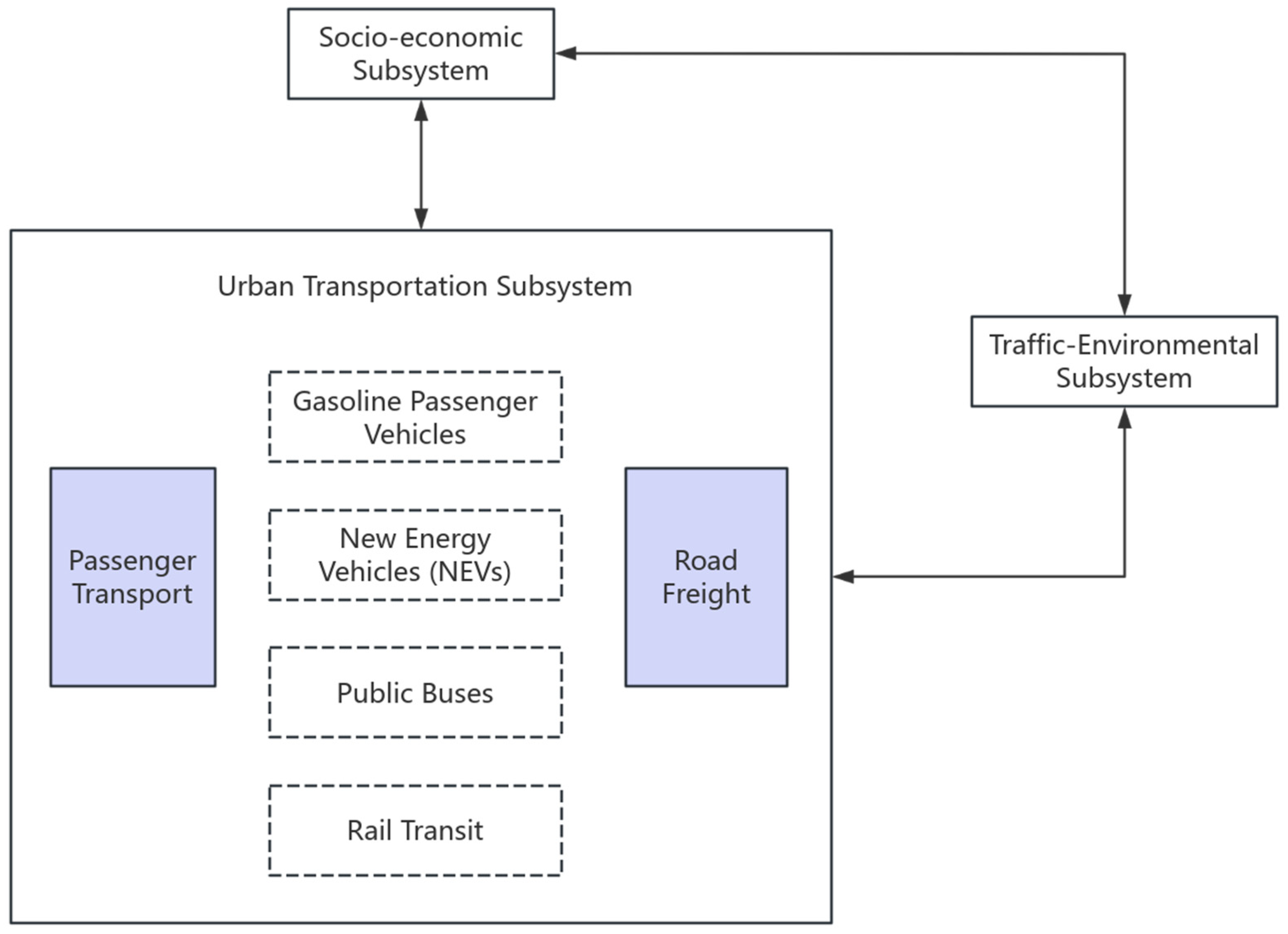
Figure 1. System boundaries.
Sustainability 17 09296 g001
Figure 2. Causal loop diagram.
Sustainability 17 09296 g002
Figure 3. Flow diagram of the socio-economic subsystem. The rectangles represent stocks (accumulations). The valves and thick arrows represent flows (rates of change). The thin arrows represent information or causal links between variables.
Sustainability 17 09296 g003
Figure 4. Flow diagram of the urban transportation subsystem.
Sustainability 17 09296 g004
Figure 5. Flow diagram of the traffic environment subsystem.
Sustainability 17 09296 g005
Figure 6. Stock-and-flow diagram of urban traffic and emissions system.
Sustainability 17 09296 g006
Figure 7. Results of extreme condition testing.
Sustainability 17 09296 g007
Figure 8. Sensitivity analysis results of key indicators under different traffic restriction policies.
Sustainability 17 09296 g008
Figure 9. Simulation results of new energy vehicle promotion policy.
Sustainability 17 09296 g009
Figure 10. Simulation results of license plate restriction policy.
Sustainability 17 09296 g010
Figure 11. Simulation results of road investment policy.
Sustainability 17 09296 g011
Figure 12. Simulation results of carpooling policy.
Sustainability 17 09296 g012
Figure 13. Simulation results of technology improvement policy.
Sustainability 17 09296 g013
Table 1. Elements of the Urban Traffic Congestion and Emission System.
SubsystemKey Factors
Socio-economicGDP growth rate, GDP, per capita GDP, total permanent resident population
Urban transportRoad capacity, freight turnover, travel volume by mode of transport, modal split, total road length, vehicle kilometers traveled by ground transport, average occupancy rate of various transport modes
Traffic EnvironmentalTotal CO2 emissions, annual vehicle emissions by pollutant type, total increment of pollutants, contribution rate of vehicles to various pollutants
Transport policyLicense plate restriction policy, new energy vehicles promotion policy, road investment policy, technology improvement policy, carpooling promotion policy
Table 2. Conceptual mechanism of transport policy.
Transport PolicySystem Impact
License plate restrictionDirectly restricts the entry and circulation of private cars, immediately reducing the total Vehicle Kilometers Traveled (VKT) and alleviating congestion.
New energy vehicles promotionAccelerates the replacement of conventional fuel vehicles. This policy alters the vehicle stock composition and subsequently lowers the aggregate emission factor for CO2 and local air pollutants.
Road investmentIncreases the physical capacity of the road network. This directly raises the overall Road Capacity, thereby improving the average travel speed and mitigating congestion.
Technology improvement Simulates the continuous upgrading of conventional engine efficiency and emission standards, resulting in a gradual reduction in emissions per VKT over time.
Carpooling promotionAims to increase the average vehicle occupancy rate. This indirectly reduces the necessary VKT per trip for the same volume of passenger travel, resulting in both congestion and emission relief.
Table 3. Energy Carbon Emission Factors.
Energy TypeGasolineDieselNatural GasElectricity
Emission Factor2.22572.54791.93880.5703
UnitkgCO2/LkgCO2/LkgCO2/m3kgCO2/(kW·h)
Table 4. Model Parameters and Initial Values.
VariableValueUnit
Urban GDP17,915.4CNY hundred million
Total Resident Population2302.66ten thousand people
Length of Major Roads300km
Length of Freeways200km
Length of Secondary and Local Roads4000km
Urban Road Investment0.002Dmnl
Average Passenger Capacity (Gasoline)1.8persons/vehicle
Average Travel Distance (Gasoline)14km
Gasoline Car Energy Consumption8.82L/100 km
Average Passenger Capacity (NEV)1.8persons/vehicle
Average Travel Distance (NEV)14km
NEV Energy Consumption15.17kWh/100 km
Average Passenger Capacity (Bus)21persons/vehicle
Average Travel Distance (Bus)12.5km
Bus Energy Consumption55.5kWh/100 km
Average Passenger Capacity (Rail)49persons/vehicle
Average Travel Distance (Rail)18.7km/person-trip
Rail Energy Consumption338.28kWh/100 km
NOx Emissions (Gasoline Cars)0.0043ton/year/vehicle
NOx Contribution Rate (Gasoline Cars)0.0897Dmnl
Number of Lanes (Major Roads)6-
Lane Capacity (Major Roads)8000vehicle-kilometers
Number of Lanes (Freeways)6-
Lane Capacity (Freeways)8000vehicle-kilometers
Number of Lanes (Secondary Roads)6-
Lane Capacity (Secondary Roads)8000vehicle-kilometers
Unit Road Construction Cost0.3CNY hundred million/km
Road Investment Conversion Rate0.15Dmnl
Table 5. Validation Results of Shanghai’s GDP (CNY Hundred Million).
YearUrban GDP
(Actual Value)
Urban GDP
(Simulated Value)
Urban GDP
(Error Value)
Error
201017,915.417,915.400.00%
201120,009.719,880.2−129.5−0.65%
201221,305.621,085.4−220.2−1.03%
201323,204.122,840.3−363.8−1.57%
201425,269.824,734.8−535−2.12%
201526,887.026,206.6−680.4−2.53%
201629,887.028,920.7−966.3−3.23%
201732,925.031,638.8−1286.2−3.91%
201836,011.834,376.6−1635.2−4.54%
201937,987.636,113.1−1874.5−4.93%
202038,963.336,965.7−1997.6−5.13%
Table 6. Validation Results of Shanghai’s Resident Population (ten thousand people).
YearResident Population
(Actual Value)
Resident Population
(Simulated Value)
Resident Population
(Error Value)
Error
20102302.662302.6600.00%
20112355.532321.33−34.2−1.45%
20122398.52332.59−65.91−2.75%
20132448.432342.46−105.97−4.33%
20142467.062351.13−115.93−4.70%
20152457.592361.35−96.24−3.92%
20162467.372368.67−98.7−4.00%
20172466.282380.68−85.6−3.47%
20182475.392391.85−83.54−3.37%
20192481.342403.43−77.91−3.14%
20202488.362414.72−73.64−2.96%
Table 7. Validation Results of Shanghai’s Daily Average Total Travel Volume (Ten Thousand Person-Times).
YearTotal Travel Volume
(Actual Value)
Total Travel Volume
(Simulated Value)
Total Travel Volume
(Error Value)
Error
201331643161.75−2.25−0.07%
201431683179.3411.340.36%
201532003200.090.090.00%
201632213214.94−6.06−0.19%
201732533239.31−13.69−0.42%
201832683261.96−6.04−0.18%
201932733285.4512.450.38%
202026123308.37696.3726.66%
Table 8. Normalized Indicator Matrix.
C1C2C3
Y110.58160
Y20.524000.3646
Y3011
Y40.59510.16670.4690
Y50.95060.72080.9919
Y60.95060.78130.9919
Table 9. Weighted Decision Matrix.
C1C2C3
Y10.30880.20700
Y20.161800.1223
Y300.35590.3353
Y40.18370.05930.1572
Y50.29350.25660.3326
Y60.29350.27810.3326
Table 10. Closeness Coefficients.
Policyd+dCloseness Coefficient CᵢRanking
Y10.37170.36690.49673
Y20.20280.44010.68451
Y30.48900.30880.38714
Y40.24900.36790.59632
Y50.51240.10060.16415
Y60.52350.07940.13176
Disclaimer/Publisher’s Note: The statements, opinions and data contained in all publications are solely those of the individual author(s) and contributor(s) and not of MDPI and/or the editor(s). MDPI and/or the editor(s) disclaim responsibility for any injury to people or property resulting from any ideas, methods, instructions or products referred to in the content.