Study on Spatiotemporal Pattern Evolution and Regional Heterogeneity of Carbon Emissions at the County Scale of Major Cities, Inner Mongolia Autonomous Region

Abstract

In-depth exploration of the spatial heterogeneity patterns of urban carbon emissions holds significant scientific importance for regional sustainable development. However, few scholars have examined the spatiotemporal characteristics of county-level carbon emissions in Inner Mongolia. This study focuses on the three major cities of Hohhot, Baotou, and Ordos in Inner Mongolia. By integrating NPP-VIIRS nighttime light data, the CLCD (China Land Cover Dataset) dataset, and statistical yearbooks, it quantifies county-level carbon emissions and establishes a spatiotemporal analysis framework of urban morphology–carbon emissions from 2013 to 2021. Six morphological indicators—Class Area (CA), Landscape Shape Index (LSI), Largest Patch Index (LPI), Patch Cohesion Index (COHESION), Patch Density (PD), and Interspersion Juxtaposition Index (IJI)—are employed to represent urban scale, complexity, centrality, compactness, fragmentation, and adjacency, respectively, and their impacts on regional carbon emissions are examined. Using a geographically and temporally weighted regression (GTWR) model, the results indicate the following: (1) from 2013 to 2021, The high-value areas of carbon emissions in the three cities show a clustered distribution centered on the urban districts. The total carbon emissions increased from 20,670 (10⁴ t/CO₂) to 37,788 (10⁴ t/CO₂). The overall spatial pattern exhibits a north-to-south increasing gradient, and most areas are projected to experience accelerated carbon emission growth in the future; (2) the global Moran’s I values were all greater than zero and passed the significance tests, indicating that carbon emissions exhibit clustering characteristics; (3) the GTWR analysis revealed significant spatiotemporal heterogeneity in influencing factors, with different cities exhibiting varying directions and strengths of influence at different development stages. The ranking of influencing factors by degree of impact is: CA > LSI > COHESION > LPI > IJI > PD. This study explores urban carbon emissions and their heterogeneity from both temporal and spatial dimensions, providing a novel, more detailed regional perspective for urban carbon emission analysis. The findings enrich research on carbon emissions in Inner Mongolia and offer theoretical support for regional carbon reduction strategies.

1. Introduction

Driven by global climate change and dual-carbon goals, urban spatial form—as the material carrier of human–natural system interactions—exhibits a critical nexus with carbon emissions, establishing itself as a pivotal research frontier for spatial optimization and low-carbon transitions. This linkage stems not only from the direct impact of urban spatial organization on energy consumption and land-use efficiency, but is further reinforced by the systematic steering of national policy frameworks.

In 2022, the National Development and Reform Commission (NDRC) of China issued the “14th Five-Year Plan for New-Type Urbanization Implementation Scheme,” which proposed optimizing the spatial layout and form of urbanization, advancing the construction of new cities, enhancing the integrated development of urban agglomerations and the coordinated development of metropolitan areas, and promoting the balanced development of large, medium, and small cities and towns [1]. In 2021, the Central Committee of the Communist Party of China and the State Council issued the “Opinions on Promoting Green Development of Urban and Rural Construction,” which emphasized the promotion of a multi-center, networked layout of urban agglomerations and metropolitan areas. The proposal also focused on optimizing spatial structure with a compact, intensive, and balanced approach to work and residence, and establishing a green, low-carbon-oriented urban renewal mechanism. Through the refined control of spatial forms, this strategy aims to curb ecological encroachment and energy waste caused by unchecked urban expansion [2].

Evidently, as China undergoes structural advancement in urbanization, investigating dynamic response mechanisms between urban spatial morphology and carbon emissions constitutes a crucial pathway for reconciling urbanization–ecological constraints, while providing scientific underpinnings for constructing high-quality development spatial frameworks.

As China’s strategic energy base and northern ecological security barrier, Inner Mongolia features a “large dispersion, small concentration” spatial pattern in its major cities (Hohhot-Baotou-Ordos) shaped by resource endowments. During rapid urbanization, these cities function both as regional economic growth poles and concentrated carbon emission zones, where spatial heterogeneity systematically shapes regional emission patterns.

2. Literature Review

Against the backdrop of global climate change and dual-carbon objectives, urban carbon emission research has yielded significant advances. However, the existing research still has significant limitations, which restrict the comprehensive understanding and effective response to the carbon emission issues of Hohhot-Baotou-Ordos cities. The constraints are principally evident at three levels:

At the level of research scale, scholars have examined the relationship between urban carbon emissions and spatial morphology across different regional scales. At the national scale, some scholars have analyzed the evolution of urban spatial morphology across China’s 264 urban agglomerations [3]. At the provincial scale, the Pearl River Delta, one of the most rapidly developing and economically advanced regions in China, has frequently been used for time-series analyses of carbon emissions. For example, Wang et al. [4] examined all nine cities in the Pearl River Delta, using panel data from 1990 to 2013 to reveal the relationship between urban morphology and CO₂ emission efficiency. Similarly, in rapidly growing and relatively developed regions, some scholars have selected provincial capital cities as the focus to analyze the relationship between urban carbon emissions and spatial morphology. For instance, Ou [5] used time-series data from 1990 to 2010 to quantify the relationship between urban form and carbon emissions in four of China’s fastest-growing cities: Beijing, Shanghai, Tianjin, and Guangzhou. Using the same time series, Fang et al. [6] analyzed panel data from 30 provincial capital cities in China between 1990 and 2010, finding a positive correlation between urban area expansion and CO₂ emissions. At the city scale, Falahatkard et al. [7] investigated 15 cities in Iran to quantify the relationship between CO₂ emissions and urban morphology. Their findings suggest that making existing northern Iranian cities more compact could, in fact, help reduce carbon emissions. Clearly, most existing studies focus on macro-level regions such as national, provincial, or large city scales, and typically target large or densely populated urban areas. There is limited attention to spatial forms in regions that overlap ecologically fragile and energy-rich zones. In particular, there is a lack of fine-grained analysis of the carbon effects of urban spatial forms at the county level, making it difficult to accurately identify regional emission characteristics and mitigation potential. The primary reason for this gap is the difficulty in obtaining county-level carbon emission data and the challenges associated with accurately calculating emissions at such a refined scale. In recent years, with the advancement of remote sensing technology, the use of nighttime light data has become increasingly diversified. Some scholars have combined nighttime light data with carbon emissions and employed fitting methods to estimate carbon emissions in certain regions [8,9,10]. As one of the most frequently used datasets in recent years, NPP-VIIRS data is favored by scholars for its higher spatial resolution, strong radiometric calibration, and good temporal continuity. In the field of carbon emission analysis, some scholars have fitted NPP-VIIRS data with county-level CO₂ emission inventories to construct carbon emission models at both grid and pixel scales [11]. Others have used NPP-VIIRS data to map CO₂ emissions from urban residential areas at high spatial resolution [12]. At the county scale, Zhu et al. [13] integrated NPP-VIIRS with DMSP-OLS nighttime light data to construct a long-term county-level dataset for China, thereby improving temporal consistency. At the same scale but with a regional focus, other scholars conducted analyses that revealed the spatiotemporal patterns of carbon emissions in Northeast China [14]. Nighttime light data can also support multi-level spatial analyses, such as city–district–street scales [15] or national–urban agglomeration–suburban scales [16]. Thus, nighttime light data effectively compensate for the limitations of insufficient energy statistics in estimating carbon emissions at finer scales. They enable downscaling analyses of emissions and provide a reliable approach for estimating carbon emissions at the county level in Inner Mongolia’s cities.

Regarding carbon emissions and their driving factors in Inner Mongolia, some scholars have focused on urban population, labor force, and labor productivity [17], while others have emphasized city-level population, per capita GDP, and energy intensity [18]. Additional studies have examined economic growth rate, urbanization, industrial structure, and road density [19,20]. These findings suggest that most existing research emphasizes economic and social drivers. Moreover, long-term time-series analyses help to better reveal the evolution of carbon emissions and spatial drivers. For example, Du et al. [21] analyzed the spatiotemporal variation and driving factors of land-use carbon emissions in Xilin gol, Inner Mongolia, from 1990 to 2020. Gao et al. [22] systematically examined the coupling and coordination relationship between land-use carbon emissions (CELU) and high-quality economic development (HQED) from 2000 to 2020. Analyses of influencing factors have also shown that economic level is the most important determinant of household carbon footprints [23]. Meanwhile, Yang et al. developed a “driving–prediction–simulation” framework for carbon emissions in Hohhot, Baotou, and Ordos. Their results indicated that population and urbanization are the primary drivers of carbon emissions, followed by economic development and industrial energy consumption [24]. Overall, existing studies on the driving factors of carbon emissions in Inner Mongolia have largely concentrated on economic and social aspects, with relatively little attention to the impact of urban spatial morphology. Research proposing mitigation strategies from the perspective of urban planning and morphological structure remains scarce.

In terms of research methodology, studies on carbon emissions and their driving factors employ a wide range of approaches, with quantitative analysis being the most common. The Logarithmic Mean Divisia Index (LMDI) decomposition model can clearly attribute the contributions of different drivers to carbon emissions. Its results are intuitive and suitable for multi-period comparisons, but it fails to capture spatial differences and is limited in analyzing spatiotemporal interactions [17,18]. Some studies have further applied Grey Relational Analysis (GRA) on the basis of the LMDI method to examine the relationship between carbon emissions and GDP growth [25]. For forecasting carbon emissions in Inner Mongolia, the STIRPAT model has been applied to extend the range of explanatory indicators [24,26]. This approach incorporates multiple driving factors and enables scenario-based projections, making it suitable for urban agglomeration studies. However, the temporal dimension is typically treated only as a trend, without accounting for local spatiotemporal variations. With respect to spatial regression, the Geographically Weighted Regression (GWR) model can identify spatial heterogeneity across regions, with coefficients offering spatial interpretability. For example, some scholars have used GWR to quantify the spatially non-stationary responses of carbon sequestration and ecosystem health drivers in Inner Mongolia [27,28]. However, these methods overlook the temporal dimension of spatial heterogeneity in carbon emissions, limiting their ability to analyze time-series dynamics. The Geographically and Temporally Weighted Regression (GTWR) model simultaneously accounts for both spatial and temporal dimensions, thereby overcoming the limitations of traditional approaches in capturing time-series variations. Studies applying GTWR to carbon emissions and their determinants have revealed significant spatiotemporal heterogeneity in the effects of urban morphology, with the magnitude of influence varying across different stages [29,30]. These findings suggest that policies should be tailored to local conditions and adjusted over time to support sustainable urban development. Moreover, applications of GTWR are expanding beyond macro-level studies of total carbon emissions [31] to encompass urban agglomerations [32], residential buildings [33], and land use [34]. The indicator systems employed have also broadened from purely socioeconomic factors to include infrastructure, ecosystem health, and other multidimensional aspects. Overall, the GTWR model demonstrates strong adaptability and a solid research foundation for examining the drivers of carbon emissions across multiple scales and indicators, providing valuable theoretical support for understanding urban carbon emission mechanisms.

Targeting the Hohhot-Baotou-Ordos urban cluster in Inner Mongolia at the county scale, this research couples spatial morphology metrics with carbon accounting models to unravel dynamic causal pathways through which urban spatial structure and functional configurations influence carbon emissions. The study aims to provide scientific foundations for optimizing spatial governance in ecologically sensitive border cities, reconciling ecological conservation with low-carbon development, while contributing to theoretical advances in context-responsive planning frameworks under the dual-carbon goals.

3. Materials and Methods

3.1. Study Area

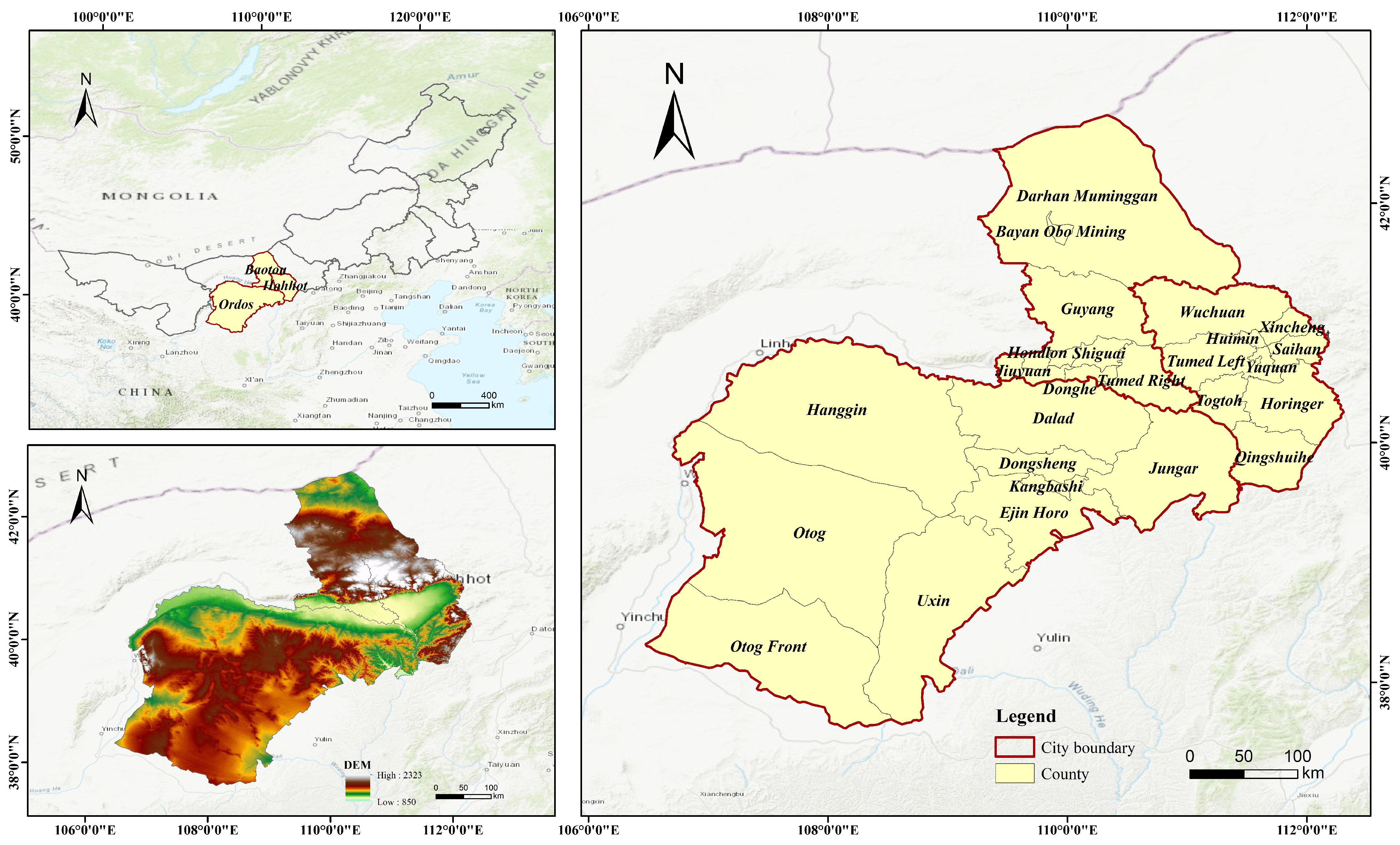
Hohhot, Baotou, and Ordos (collectively termed HBO) are situated in central Inner Mongolia Autonomous Region, administering 12 districts, 5 counties, and 10 banners (Figure 1). Situated in the transitional zone between the Loess Plateau and the grasslands, the region features complex geography, diverse topography, and a typical temperate continental climate. The area experiences low precipitation, an arid climate, distinct seasonal variations, and large diurnal temperature differences. Geographically, the three cities form a triangular configuration with close spatial proximity. Relying on the Yellow River’s water resources and the agricultural foundation of the Hetao Plain, they support industrial and urban development. This area is the most economically dynamic and promising region in Inner Mongolia, often referred to as the “Golden Triangle” of the region.

Economically, HBO serves as both the economic core of Inner Mongolia and a regional growth pole. In 2021, the GDPs of Hohhot, Baotou, and Ordos were 312.14 billion yuan, 329.30 billion yuan, and 135.48 billion yuan, respectively, accounting for a total of 38.4% of the province’s GDP. They ranked among the top three in the entire region. In terms of industrial structure, Hohhot, the political, economic, and cultural center of the autonomous region, is dominated by modern service industries and the dairy sector. Baotou, as an established industrial base, is centered on four pillar industries: rare earths, crystalline silicon photovoltaics, steel, and aluminum. Ordos, leveraging its world-class energy sector, coal-to-chemical industry, and cashmere production, has become a major industrial hub in China. As industrial structures in HBO continue to optimize and regional cooperation deepens, the three cities have engaged in extensive collaboration in public services, infrastructure, technological innovation, and ecological governance. These synergies have significantly enhanced regional competitiveness, driven by the joint effects of industrial development, policy orientation, and resource endowment.

With their favorable geographical location, abundant resources, and developed transportation networks, the HBO cities have become a key economic growth pole in both Inner Mongolia and northern China. Through industrial collaboration and integrated infrastructure development, the three cities are progressively evolving into a modern urban agglomeration. However, this growth is accompanied by rising energy consumption and carbon emissions, further exacerbating the challenges between development and resource–environment constraints.

3.2. Data

(1)

Energy consumption, population, and GDP data for Hohhot, Baotou, and Ordos were sourced from the Inner Mongolia Statistical Yearbook (2014–2022) [35], Hohhot Statistical Yearbook (2014–2022) [36], Baotou Statistical Yearbook (2014–2022) [37], and Ordos Statistical Yearbook (2014–2022) [38].

(2)

The NPP-VIIRS nighttime light data were obtained from the Earth Observation Group at the Colorado School of Mines (VIIRS Nighttime Light (mines.edu)) [39]. This study selected the 2013–2021 VCM (Cloud-Free Monthly Composites, excluding stray light-affected data) long-term global stable nighttime light monthly datasets. The spatial resolution of the data is 500 m × 500 m, and the data were calibrated prior to analysis. The data calibration process can be found in the Appendix A of the article.

(3)

Land use data for Hohhot, Baotou, and Ordos were sourced from the China Land Cover Dataset (CLCD) (2013–2021), developed by the research team led by Yang Jie at Wuhan University [40]. This dataset was created using 335,709 Landsat images from Google Earth Engine, combined with machine learning and post-processing techniques. It includes nine land use types, such as impervious surfaces, croplands, forests, and others. This study uses impermeable surfaces as urban built-up areas to analyze changes in urban spatial form.

3.3. Methods

3.3.1. Carbon Emission Estimation and Temporal Prediction

(1)

Carbon emission estimation

The study first applies the Kaya identity to calculate carbon emissions in the Hohhot-Baotou-Ordos urban agglomeration in Inner Mongolia, and then uses nighttime light data to estimate carbon emissions at the county level. The Kaya Identity, first proposed by Yoichi Kaya (1989) in a seminar of the Intergovernmental Panel on Climate Change (IPCC), involves four factors, comprising the energy carbon emission coefficient, energy intensity, GDP per capita and population size—providing an intuitive description of the relationship between human activity and greenhouse gas emissions [41].

$$C=P\times \left({\displaystyle \frac{GDP}{P}}\right)\times \left({\displaystyle \frac{E}{GDP}}\right)\times \left({\displaystyle \frac{{CO}_2}{E}}\right)$$

(1)

where C denotes the urban carbon emissions; P is the total urban population; GDP represents the gross domestic product; E is the total energy consumption; and CO₂/E indicates the carbon emissions per unit of energy consumption, calculated after con-verting fuel consumption to standard coal equivalent. Based on the energy consumption structure of the Hohhot-Baotou-Ordos urban agglomeration, the study uniformly adopts standard coal equivalent converted from raw coal for calculating total energy-related carbon emissions. The carbon emission factors are referenced from the IPCC Guidelines [42].

To obtain carbon emission values at the county scale, considering the correlation between nighttime light data and carbon emissions, three linear regression models were constructed to fit the total brightness values of NPP-VIIRS nighttime light data against the corresponding annual energy consumption carbon emissions for the three cities from 2013 to 2021. The resulting fitted equations for energy consumption carbon emissions in HBO are presented in Figure 2.

The results indicate a strong correlation between nighttime light data and energy-related carbon emissions, with goodness-of-fit values R² all above 0.85 and significance levels p < 0.01, supporting the use of nighttime light data for county-scale carbon emission estimation in the HBO region.

The county-level carbon emissions in HBO are estimated by proportionally allocating emissions based on the ratio of the county’s total nighttime light brightness to that of the corresponding city [43,44]. The calculation formula is as follows:

$$C_{i,t}=C_{n,i,t}\times {\displaystyle \frac{{TDN}_{i,t}}{{TDN}_{n,i,t}}}$$

(2)

In the formula, $C_{i,t}$ represents the carbon emissions of region i in year t; $C_{n,i,t}$ denotes the total carbon emissions of the city n to which region i belongs in year t; ${TDN}_{i,t}$ is the total nighttime light brightness value of region i in year t; and ${TDN}_{n,i,t}$ is the total nighttime light brightness value of city n (where region i is located) in year t.

(2)

Temporal prediction

To analyze the temporal scaling behavior of county-level CO₂ emissions, we adopted the time-averaged mean-squared displacement (TAMSD) framework, following Cherstvy et al. [45]. For each county, the calculation formula for TAMSD is as follows:

$$\overline{{\delta }^2(∆)}={\displaystyle \frac{1}{T-∆}}\sum _{t=1}^{T-∆}{(E_{t+∆}-E_t)}^2$$

(3)

where $E_t$ denotes the annual CO₂ emissions in year $t$, $T$ is the series length (2013–2021), and $\Delta$ is the time lag.

Then fitted the TAMSD to a power-law form:

$$\overline{{\delta }^2(∆)}~{∆}^{\propto }$$

(4)

by linear regression in log–log coordinates. The slope $\alpha$ represents the temporal scaling exponent: $\alpha \approx 1$ indicates normal linear growth, $\alpha >1$ accelerated growth, and $0<\alpha <1$ decelerated growth. Counties with $\alpha <0$ or with poor fit quality (low $R^2$) were considered not to follow a power-law scaling and excluded from further interpretation.

3.3.2. Selection of Urban Spatial Form Indicators

Urban spatial form refers to the distribution, configuration, and structural characteristics of the built environment in physical space. It provides a critical lens for understanding urban development and environmental sustainability. The selection of spatial form indicators must align closely with the characteristics of urban development and planning objectives. Through the integrated analysis of multidimensional indicators, a scientifically sound index system can be constructed to reveal spatial patterns and support sustainable development decision-making. Based on existing research and the specific morphological features of the HBO urban region in Inner Mongolia, this study evaluates the urban spatial form and its evolution at the county level from 2013 to 2021 using six key indicators: CA, LSI, LPI, COHESION, PD, and IJI. Among these, CA and LSI reflect the overall spatial structure; LPI and COHESION highlight the efficiency of spatial organization; while PD and IJI reveal micro-level land coordination.

Descriptions of each indicator are provided in

Table 1. Urban Spatial Form Indicators and Their Descriptions.

Spatial Form Index	Abbreviation	Meaning of Representation	Description
Class Area	CA	Urban Scale	Total urban land area. Larger values indicate a greater degree of urban spatial expansion. Range: CA > 0.
Landscape Shape Index	LSI	Urban Complexity	Reflects the irregularity of the urban shape. Higher values indicate greater complexity and irregularity; lower values indicate more regular shapes. Range: LSI ≥ 1.
Largest Patch Index	LPI	Centrality	Proportion of the largest patch in the built-up area, indicating its spatial dominance or aggregation. Range: 0 < LPI ≤ 100.
Patch Cohesion Index	COHESION	Compactness	Measures spatial connectivity and aggregation of similar urban patches. Higher values imply a more compact urban form. Range: 0 < COHESION ≤ 100.
Patch Density	PD	Fragmentation	Number of patches per unit area, indicating the fragmentation level of land use. Range: PD > 0.
Interspersion Juxtaposition Index	IJI	Land-Use Adjacency	Indicates the evenness of urban land distribution across the landscape. Lower values suggest adjacency with fewer land-use types. Range: 0 < IJI ≤ 100.

, and all indicators were calculated using the software Fragstats4.2.

3.3.3. Spatial Autocorrelation Analysis of Carbon Emissions

Spatial autocorrelation analysis is applied to reveal the spatial association and heterogeneity of regional carbon emissions. This study employs both global and local spatial autocorrelation methods to examine the county-level carbon emission patterns in the HBO area. The Global Moran’s I measures overall spatial correlation, ranging from –1 to 1: values greater than 0 indicate clustering, values less than 0 indicate dispersion, and 0 represents no correlation. The Local Moran’s I further identifies spatial structures within counties: positive values correspond to “high–high” or “low–low” clusters, while negative values indicate “high–low” or “low–high” differences, reflecting intra-regional spatial heterogeneity.

The calculation formulas are provided in Equations (5) and (6).

$$I_G={\displaystyle \frac{n\sum _{i=1}^n\sum _{j=1}^n{w}_{ij}(x_i-\overline{x})(x_j-\overline{x})}{\left(\sum _{i=1}^n\sum _{j=1}^n{w}_{ij}\right)\sum _{i=1}^n{(x_i-\overline{x})}^2}}$$

(5)

$$I_L={\displaystyle \frac{n(x_i-\overline{x}){\sum }_{j=1}^n{w}_{ij}(x_j-\overline{x})}{\sum _{i=1}^n{(x_i-\overline{x})}^2}}$$

(6)

where $I_G$ represents the Global Moran’s I index, The Global Moran’s I index is denoted by $I_{G }$, and $I_L$ denotes the Local Moran’s I index. n is the number of the population of county-level administrative units. $w_{ij}$ denotes the spatial weight between unit i and unit j. $x_i$ and $x_j$ are the carbon emissions of the ith and jth county-level units, respectively; and $\overline{x}$ represents the average carbon emissions across all units.

3.3.4. GTWR Model

The core advantage of the GTWR model over the GWR model lies in its incorporation of the “time dimension,” which enables it to simultaneously capture the spatial heterogeneity and temporal non-stationarity of influencing factors. By accounting for temporal effects while capturing geographic location characteristics, the GTWR model satisfies the demands of complex spatiotemporal data analysis. In this study, the GTWR model is employed to analyze the spatiotemporal relationship between urban form and carbon emissions in the HBO urban cluster. The model is expressed as follows:

$$Y_i={\beta }_0({\mu }_i,{\upsilon }_i,t_i)+\sum _{j=1}^p{\beta }_j({\mu }_i,{\upsilon }_i,t_i)X_{ij}+{\epsilon }_i$$

(7)

In the equation, Yi denotes the dependent variable for the i-th region, where (μ_i,υ_i,t_i) represents the spatiotemporal coordinates of spatial point i. The term β₀(μ_i,υ_i,t_i) indicates the spatially and temporally varying intercept, while X_ij corresponds to the j-th explanatory variable in region i. The coefficient β_j(μ_i,υ_i,t_i) captures the regression parameter for the j-th explanatory variable at location i, with p specifying the total number of influencing factors; ε_i constitutes the model’s error term.

4. Results

4.1. The Spatiotemporal Evolution and Prediction of Carbon Emissions

4.1.1. Validation of County-Level Emissions Results

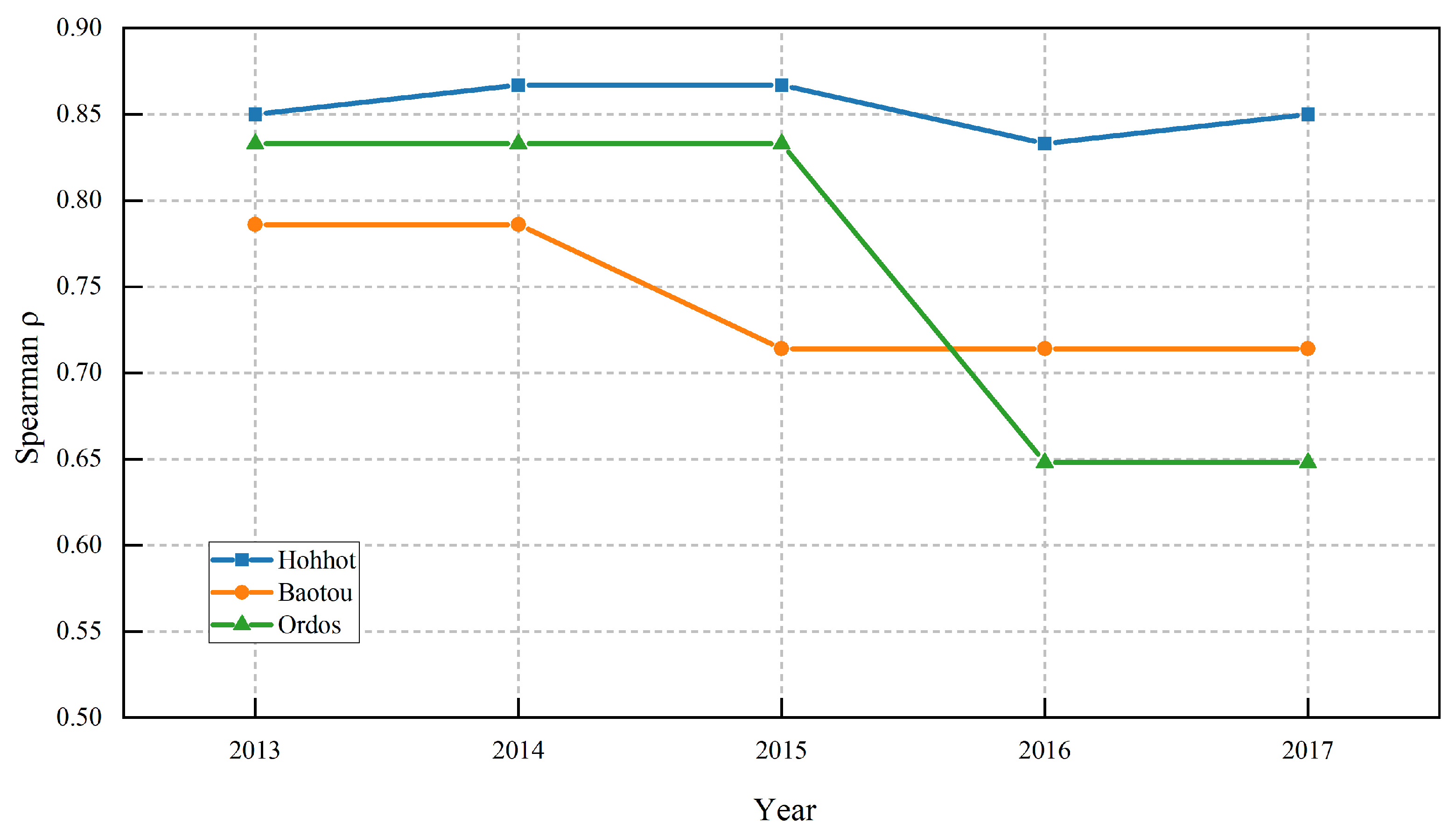
To verify the reliability of the county-level carbon emission downscaling results, this study used the dataset of Chen et al. [46] as a reference and conducted a rank correlation test for the HBO region during 2013–2017. To eliminate the influence of intercity differences in total emissions, both datasets were normalized at the county level, and the Spearman correlation coefficient (ρ) was calculated. The results (Figure 3) show that the rank correlation coefficients remained consistently high from 2013 to 2017—ranging from 0.85 to 0.87 for Hohhot, 0.71 to 0.79 for Baotou, and 0.65 to 0.83 for Ordos—all with p < 0.05. The stable and strong correlations indicate that the downscaling results are highly consistent with the external dataset in terms of spatial distribution patterns.

After the coverage period of the reference dataset, this study further evaluated the temporal robustness of the model by using 2017 as the baseline year and performing annual rank correlation tests on county-level emission share sequences from 2018 to 2021. The results show that the Spearman correlation coefficient (ρ) between 2017 and each subsequent year equals 1, indicating a perfectly consistent spatial ranking of county-level carbon emissions across the later years. This consistency largely reflects the relative short-term stability of urban spatial morphology and industrial structure in the HBO region, as well as the limited variation in the proportion of nighttime light intensity. Combined with the earlier external validation, these findings demonstrate that the model exhibits not only strong external comparability in spatial allocation but also excellent temporal consistency and structural robustness.

Spatial regression results may be influenced by the Modifiable Areal Unit Problem (MAUP), where different spatial aggregation or zoning schemes can change statistical outcomes. This study uses the county level as the analysis unit, which balances spatial detail and data availability. To reduce MAUP effects, all analyses were based on consistent county boundaries across years, and the spatial consistency of the downscaled emissions was checked. Although MAUP cannot be fully avoided, the stable spatial trends suggest its impact on the results is limited.

4.1.2. Spatiotemporal Evolution Characteristics of Carbon Emissions

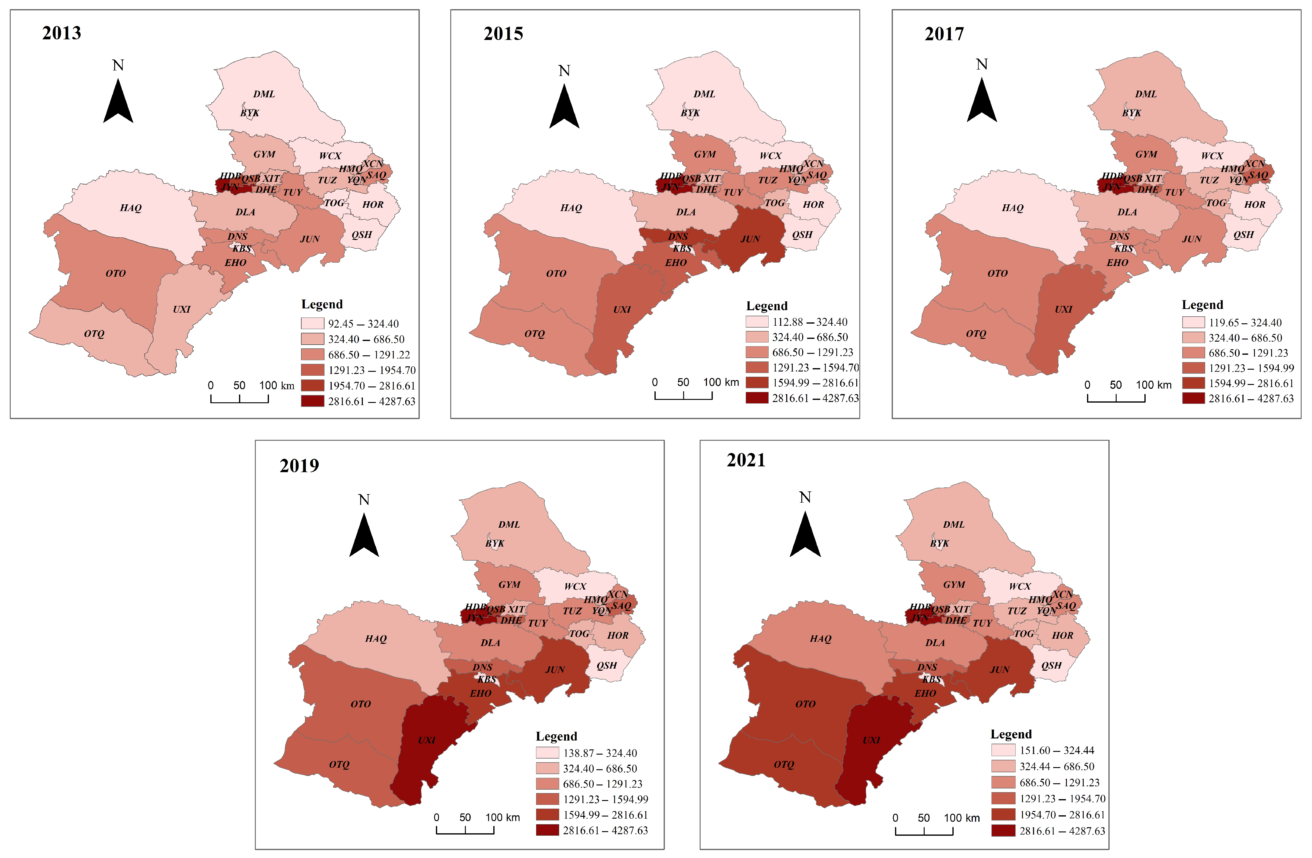
From 2013 to 2021, the total county-level carbon emissions in the HBO region increased markedly, rising from 20,670 (10⁴ t/CO₂) in 2013 to 37,788 (10⁴ t/CO₂) in 2021, representing a cumulative growth of 82.8% and an average annual growth rate of 7.8% (

Table 2. County-Level Carbon Emissions in the HBO Region from 2013 to 2021 (Unit: 10⁴ t).

Year	2013	2014	2015	2016	2017	2018	2019	2020	2021
Min	92.45	103.64	112.88	108.08	119.65	119.96	138.87	143.44	151.6
Max	2902.36	2967.6	3146.1	3373.29	3274.85	3426.17	3414.51	3549.06	4287.63
Mean	765.55	913.19	941.43	965.44	870.84	1012.17	1132.8	1233.9	1399.57
Std	699.14	746.72	783.08	823	770.21	852.37	900.53	980.46	1146.15

). The temporal evolution can be divided into two distinct phases. From 2013 to 2017, emissions grew steadily from 20,670 (10⁴ t/CO₂) to 23,513 (10⁴ t/CO₂), an increase of 13.8% with an average annual growth rate of approximately 3.3%. During this period, accelerated industrialization and urbanization expanded construction land and drove up energy demand, though the overall growth remained relatively moderate. The increase was primarily driven by the steel and coal industries concentrated in Hondlon and Jungar districts of Baotou, which together accounted for 53.1% of the city’s emissions. From 2017 to 2021, the region entered a phase of rapid growth, with total emissions surging by 60.7% within just four years and the average annual growth rate soaring to 12.5%, far exceeding that of the previous stage. The primary cause was the lag in energy consumption restructuring in Ordos, where the expansion of coal-to-chemical and other energy-intensive industries led to a rise in energy use per unit of GDP, thereby becoming the core driver of the emission surge. The temporal staging of emission growth reflects the spatial differentiation of industrial configuration and energy structure across the region (Figure 4).

In spatial terms, from 2013 to 2017, emissions were characterized by a pronounced single-core cluster centered on Hondlon and Jiuyuan districts in Baotou. By 2017–2021, the pattern had evolved into a dual-core and multi-nodal distribution, with Baotou in the north and Ordos in the south serving as the two major centers. Several counties in Hohhot (e.g., Wuchuan and Qingshuihe) maintained persistently low emission levels due to industrial hollowing-out. Overall, the regional pattern formed a three-tier gradient of “low in the north–high in the center–high in the south,” which was strongly coupled with the spatial heterogeneity of industrial distribution and energy structure.

4.1.3. TAMSD-Based Prediction of Carbon Emissions

Figure 5 illustrates the temporal growth trends of carbon emissions across the 27 counties, with most counties showing a steady increase in emissions. Based on carbon emission data from 2013 to 2017, the time-averaged mean-square displacement (TAMSD) for each county was calculated, followed by logarithmic regression analysis. The results are presented in Figure 6. The α values range from −0.53 to 1.78, with an average of 1.25. Among the 27 counties in HBO, 20 counties have α values greater than 1, while 7 counties have α values less than 1, including 2 with α < 0. For counties with α < 0, the coefficient of determination (R²) is below 0.5, indicating very poor goodness-of-fit. This suggests that the power-law model cannot adequately describe their TAMSD curves; hence, these cases are not shown in the figure. Overall, most counties in the HBO metropolitan area are projected to exhibit accelerated growth in the future, with carbon emissions expected to show active and highly volatile fluctuations. In contrast, a small number of counties are expected to experience a slowdown in growth, with carbon emissions remaining relatively stable.

4.2. Spatiotemporal Evolution of Urban Spatial Form

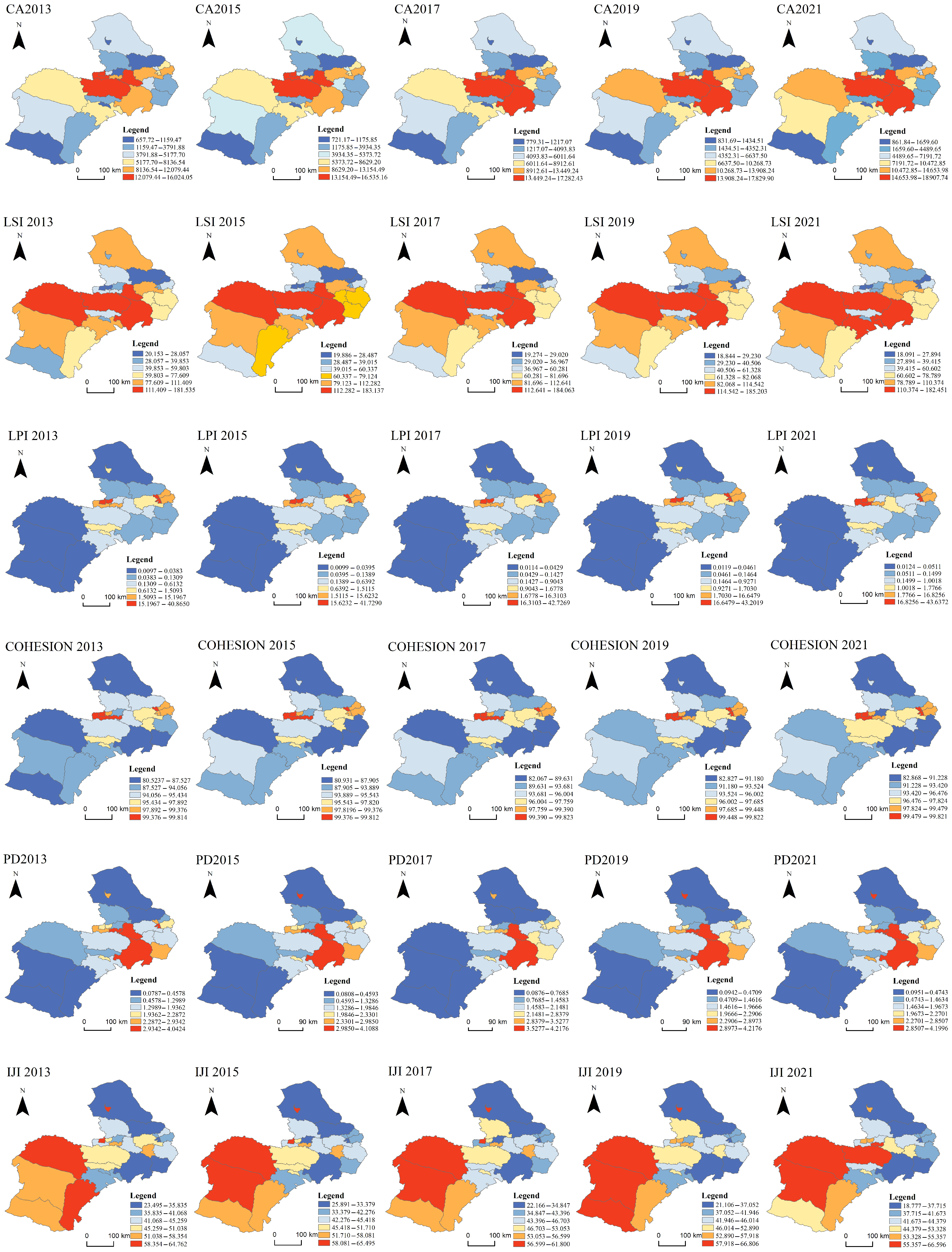
As shown in Figure 7 and

Table 3. Statistics of Spatial Form Indicators from 2013 to 2021.

Year	Statistics	Explanatory Variable
		CA	LSI	LPI	COHESION	PD	IJI
2013	Min	657.72	20.153	0.01	80.524	0.079	23.495
	Max	16,024.05	181.535	40.865	99.814	4.042	64.762
	Mean	6096.09	65.273	5.425	94.162	1.75	45.719
	Std	4428.636	39.248	9.566	5.153	1.093	10.528
2015	Min	721.17	19.886	0.01	80.931	0.081	25.891
	Max	16,535.16	183.137	41.729	99.812	4.109	65.495
	Mean	6523.51	66.423	5.617	94.425	1.789	45.883
	Std	4724.915	39.771	9.861	4.923	1.088	10.444
2017	Min	779.31	19.274	0.011	82.067	0.088	22.166
	Max	17,282.43	184.063	42.727	99.823	4.173	61.8
	Mean	7025.367	67.428	5.851	94.647	1.791	45.753
	Std	5106.144	40.53	10.142	4.671	1.08	10.031
2019	Min	831.69	18.844	0.012	82.827	0.094	21.106
	Max	17,829.9	185.203	43.202	99.822	4.218	66.806
	Mean	7478.757	68.917	6.125	94.909	1.839	46.637
	Std	5393.017	41.516	10.577	4.359	1.12	10.619
2021	Min	861.84	18.091	0.012	82.868	0.095	18.777
	Max	18,907.74	182.451	43.637	99.821	4.2	66.596
	Mean	7872.583	67.005	6.222	95.05	1.796	45.451
	Std	5672.865	40.46	10.701	4.328	1.079	10.092

, the Hohhot–Baotou–Ordos urban agglomeration experienced substantial urban expansion between 2013 and 2021. The mean CA increased from 6096 to 7872.6, representing an overall growth rate of 29.1%. At the county scale, high CA values were concentrated in Jiuyuan District, Hondlon District, Tumed Right Banner in Baotou, and Dalad Banner in Ordos.

The overall mean LSI exhibited a fluctuating upward trend, indicating increasingly complex urban forms. From 2013 to 2019, the mean LSI gradually increased, with high-value areas concentrated in Hanggin Banner, Dalad Banner, and Jungar Banner in Ordos, as well as Tumed Right Banner in Baotou. A slight decline was observed between 2019 and 2021, where the changes in Hanggin and Dalad Banners were linked to ecological fragility and human interventions, while Jungar Banner was mainly influenced by open-pit mining.

The mean LPI increased from 5.43 to 6.22, suggesting that a monocentric expansion model dominated, with intensified concentration of spatial resources, which may exacerbate issues such as traffic congestion. High LPI values were clustered in Hondlon, Qingshan, Jiuyuan, and Donghe districts of Baotou, as well as Huimin, Yuquan, Xincheng, and Saihan districts of Hohhot.

The mean COHESION increased from 94.2 in 2013 to 95.1 in 2021, reflecting enhanced land patch connectivity and increasingly compact urban development. High-value areas were mainly concentrated in the central urban districts of Hohhot and Baotou.

The mean PD rose from 1.75 in 2013 to 1.84 in 2019, before falling back to 1.80 in 2021, indicating that fragmentation intensified during the rapid expansion period but was later moderated through planning interventions. Localized high PD values appeared in Tumd Right Banner, Donghe District, and Bayan Obo Mining District of Baotou, as well as Jungar Banner in Ordos, primarily due to land use for resource extraction and fragmentation along agro-pastoral transition zones.

The mean IJI displayed a wave-like fluctuation, reflecting interannual variations in land use adjacency. High IJI values were observed in Hondlon District of Baotou, and Hanggin and Otog Banners in Ordos. In particular, the redevelopment of the former Baogang Group’s industrial site into an “industrial heritage–commercial–park” adjacency interface effectively enhanced spatial adjacency.

4.3. Influence Mechanism of Urban Spatial Form on Carbon Emissions

4.3.1. Spatial Statistical Analysis

Based on analyses conducted using the ArcGIS platform, the Global Moran’s I values for 2013–2021 were obtained (

Table 4. Global Moran’s I of carbon emissions in Hohhot, Baotou and Erdos.

Year	2013	2015	2017	2019	2021
Moran’s I index	0.2215	0.1815	0.2237	0.2213	0.2936
Z-score	2.4025	1.9665	2.4406	2.2812	2.8675
p-value	0.0163	0.0492	0.0147	0.0225	0.0041

). The Global Moran’s I values for 2013, 2015, 2017, 2019, and 2021 were all greater than 0, with absolute Z-scores exceeding 1.96 and p-values below 0.05, passing the significance test. These results indicate that carbon emissions in the HBO urban agglomeration exhibit a significant positive spatial autocorrelation, reflecting a clustered spatial pattern.

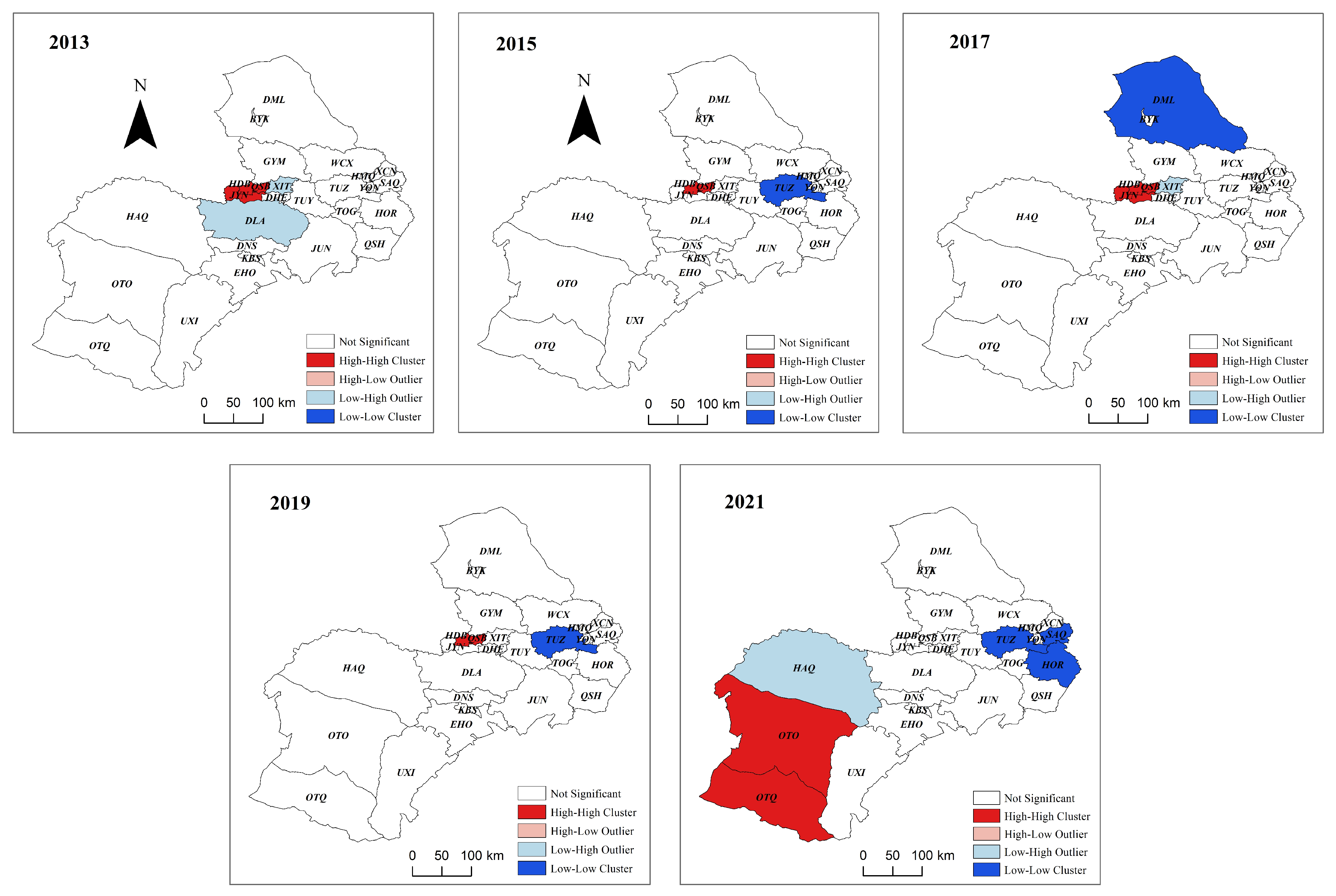
To further investigate the spatial association of carbon emissions within the HBO region, a local spatial autocorrelation analysis was conducted at the county scale. Figure 8 presents the LISA clustering results of carbon emissions in the HBO urban agglomeration from 2013 to 2021.

High-emission areas exhibit significant H–H clustering, primarily concentrated in Baotou’s central urban districts, including industrial zones, and in Ordos’ energy extraction and processing areas. These regions are the core centers of energy, industry, and population within the urban agglomeration, resulting in high carbon emission intensity. From 2013 to 2019, these clusters were relatively stable in Hondlon, Qingshan, and Jiuyuan districts of Baotou, but by 2021 they had shifted from Baotou’s central districts to southwestern Ordos, specifically Otog Front Banner and Otog Banner. This indicates that high-emission zones exhibit strong spatial persistence, largely shaped by long-term industrial layouts and energy structures.

In contrast, L–L clusters are mainly distributed in Hohhot’s non-central areas and the northern parts of Baotou. These regions are characterized by weaker economic activity and limited industrial bases, leading to overall low carbon emission levels. Notably, between 2013 and 2021, the number of L–L clusters gradually increased, most of which were concentrated in Hohhot’s non-central areas. This suggests that previously less distinct clusters are undergoing industrial and energy restructuring, showing signs of emission reduction, and warranting further attention.

L–H clusters show a declining and intermittent trend: in 2013 they appeared in Dalad Banner (Ordos) and Shiguai District (Baotou); by 2017 only in Shiguai; and in 2021 they shifted to Hanggin Banner (Ordos). These results demonstrate pronounced spatial heterogeneity in the study region, with HBO’s carbon emissions showing hierarchical clustering overall, while the spatial clustering effects of individual counties are weakening. The dominant patterns are H–H and L–L clusters, with a few L–H anomalies, indicating strong spatial dependence of carbon emissions at the local scale.

4.3.2. Data Processing and Testing

First, all spatial form variables and carbon emission data were standardized using normalization methods. Then, SPSS 27 was employed to calculate the Variance Inflation Factor (VIF) for each variable to test for multicollinearity in the regression model. The results showed that the VIF values for all six variables were less than 7, and the tolerance values were greater than 0.1. This indicates that there were no significant correlations among the variables, and multicollinearity was not present, making the dataset suitable for regression analysis (

Table 5. Multicollinearity Test Results (VIF) for Urban Spatial Form Indicators.

Variable	CA	LSI	LPI	COHESION	PD	IJI
VIF	5.069	6.564	2.727	3.400	1.411	1.151
Tolerance	0.197	0.152	0.367	0.294	0.709	0.869

Note: VIF: the variance inflation factors.

).

4.3.3. GTWR Model Results and Analysis

According to the model diagnostic indicators (

Table 6. Comparison of Model Evaluation Metrics.

Model Parameter	GTWR	GWR	TWR	OLS
R2	0.9566	0.9338	0.4719	0.4405
AICc	87.3561	109.3780	560.3970	561.4771
Bandwidth	0.1150	0.1150	0.5585	/
Residual Squares	10.5435	16.0853	128.3230	135.3923
Sigma	0.2083	0.2573	0.7267	/

), the GTWR model outperforms the GWR, TWR, and OLS models in both fitting accuracy and robustness. The coefficient of determination (R² = 0.9566) of the GTWR model is substantially higher than that of the other models, indicating its superior explanatory power for the spatiotemporal variations of carbon emissions. The AICc value is the lowest (87.36), suggesting that the model achieves high goodness of fit while avoiding overfitting. Both the residual sum of squares (10.54) and the residual standard deviation (σ = 0.208) are significantly smaller than those of the GWR model (16.09, σ = 0.257), implying smaller model errors and a more random residual distribution. The stable bandwidth parameter (0.115) further confirms good model convergence. Overall, the GTWR model demonstrates the highest robustness and best fitting performance, effectively capturing the spatial and temporal heterogeneity of carbon emissions.

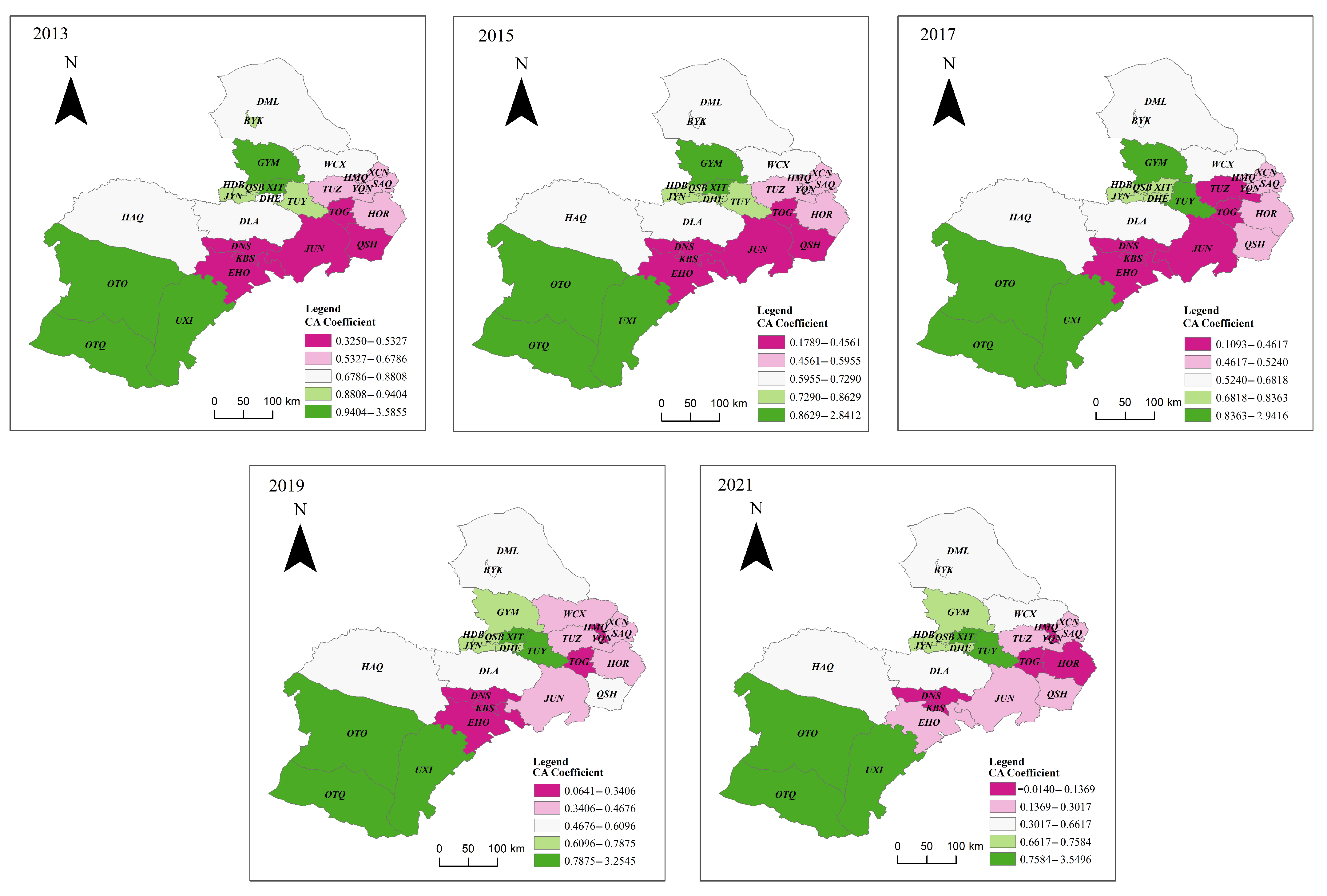
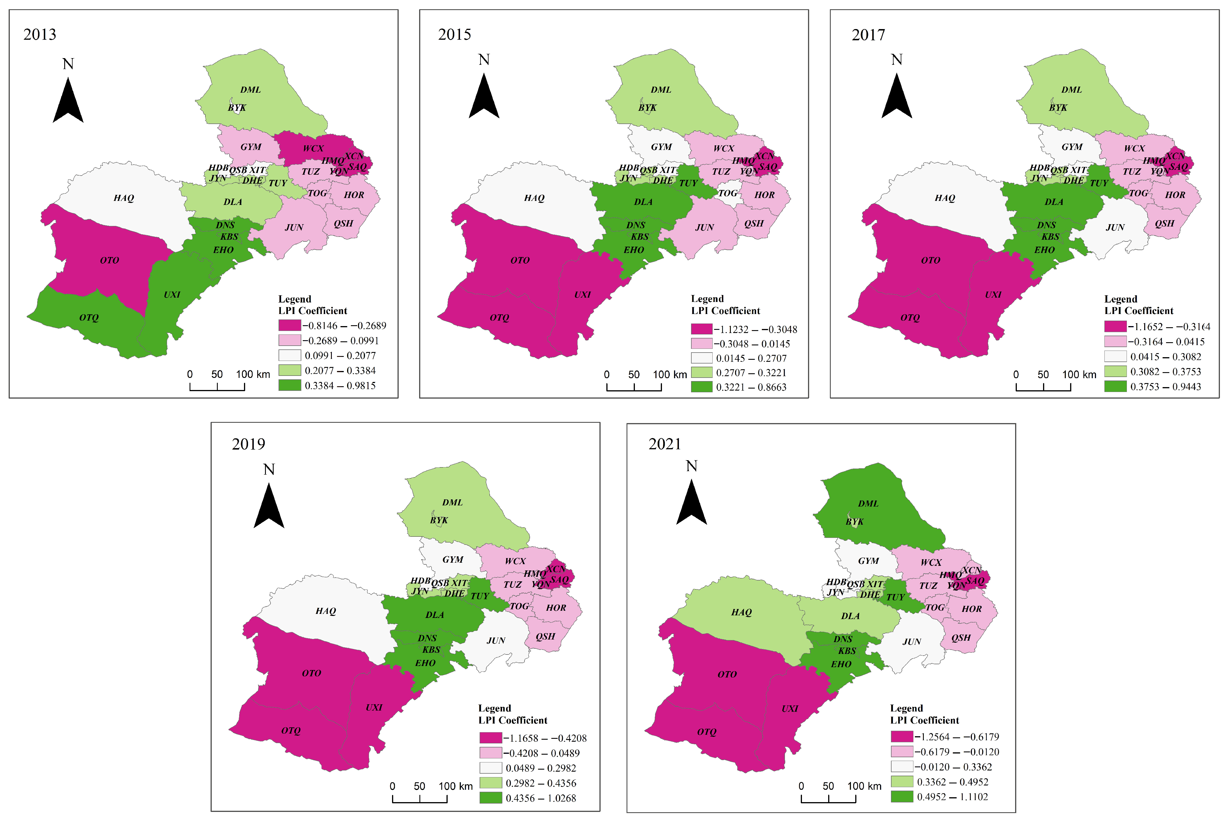
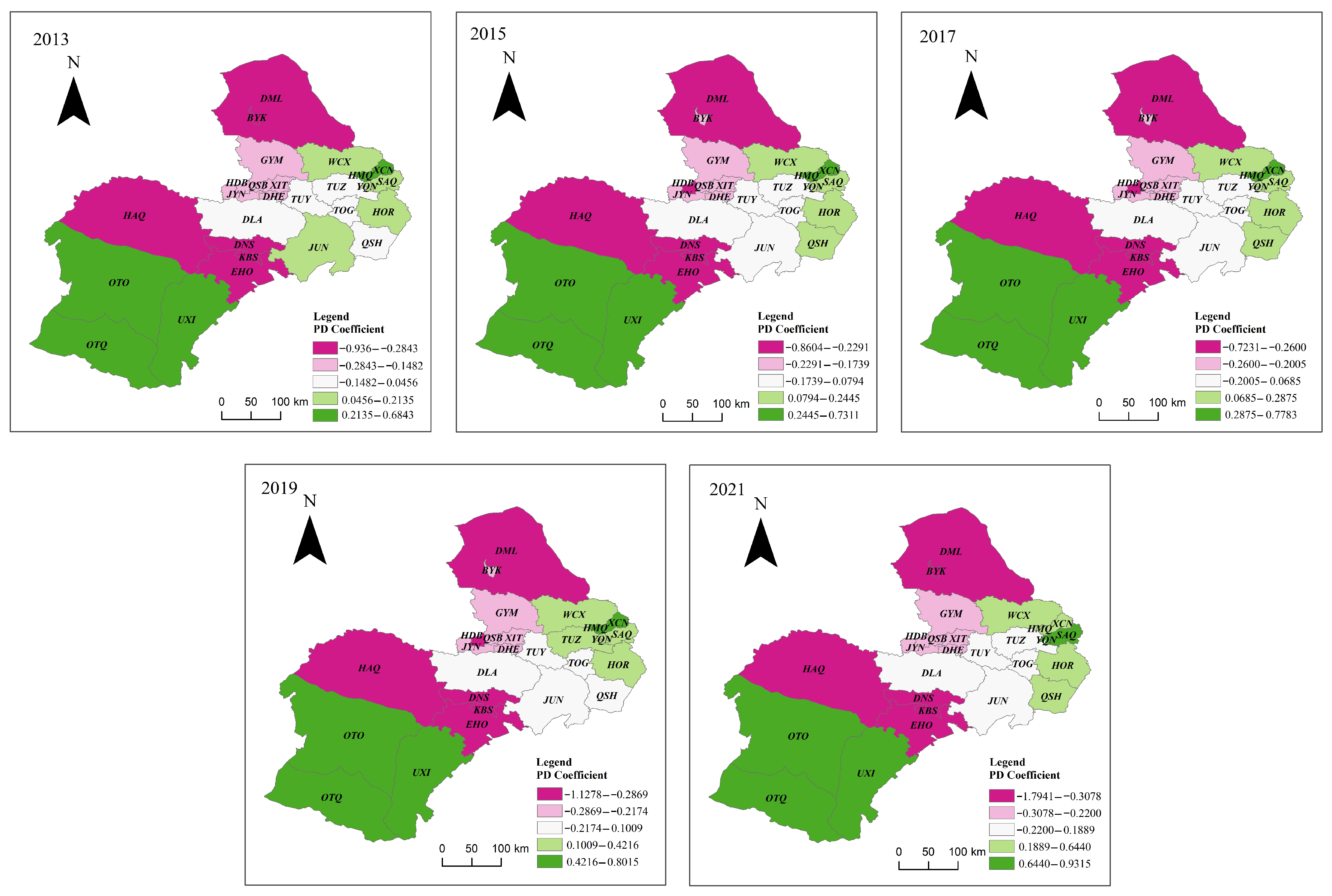
Based on the absolute values of the regression coefficients (

Table 7. Results of the GTWR Model and Descriptive Statistics of Regression Coefficients.

Influencing Factors	Min	Max	Mean (Absolute Value)	Median	Std
Class area (CA)	0.014	3.5855	0.7524	0.6198	0.6625
Landscape shape index (LSI)	−1.9673	0.7903	0.4948	−0.3579	0.4756
Largest patch index (LPI)	−1.2564	1.1102	0.4394	0.1916	0.5423
Patch cohesion index(COHESION)	−0.5651	4.1645	0.4700	0.2472	0.7151
Patch density (PD)	−1.7941	0.9315	0.3471	−0.0917	0.4369
Interspersion & Juxtaposition index (IJI)	−2.1177	0.5406	0.4375	−0.281	0.4449

), the relative influence of the factors was ranked as CA > LSI > COHESION > LPI > IJI > PD. Examination of the extreme value ranges reveals that, except for CA, the other five spatial morphological factors exhibited both positive and negative correlations with regional carbon emissions. Considering the median values, the coefficients of LPI and PD ranged from a maximum of 1.1102 and 0.9315 to a minimum of −1.2564 and −1.7941, respectively, indicating that their positive and negative effects varied across different cities. For LSI and IJI, the absolute values of the minimum coefficients were more than twice their maximum values, suggesting that their coefficients were predominantly negative and mainly exhibited inverse relationships with carbon emissions. COHESION displayed the largest variance, indicating a more widely dispersed distribution of regression coefficients.

4.3.4. Spatiotemporal Heterogeneity of Factors Influencing Carbon Emissions

Based on the regression results of the Geographically and Temporally Weighted Regression (GTWR) model, the spatial distribution of regression coefficients for six influencing factors in the years 2013, 2015, 2017, 2019, and 2021 was visualized using ArcGIS. This allows for an intuitive observation of the spatiotemporal variation in the effects of different factors on carbon emissions across the HBO, as shown in Figure 9, Figure 10, Figure 11, Figure 12, Figure 13 and Figure 14.

The spatiotemporal heterogeneity of the effect of the Urban Scale (CA) index on carbon emissions is shown in Figure 9.

From a temporal perspective, the regression coefficients between the urban scale index (CA) and urban carbon emissions from 2013 to 2021 are positive and show an overall increasing trend. This suggests that urban expansion positively affects carbon emissions, and this effect has been growing stronger over time. As the built-up area expands, carbon emissions tend to increase.

Spatially, during the period 2013–2017, regions with high absolute values of CA regression coefficients were mainly concentrated in the central part of the study area, including Shiguai District and Guyang County, as well as in the southwestern areas such as Otog Banner, Otog Front Banner, and Uxin Banner. In contrast, low-value regions were located in the eastern part of Ordos and the southern part of Hohhot. Between 2017 and 2021, the regions with high absolute values of the CA regression coefficient gradually shifted from the central part of the study area to the southeastern region. Meanwhile, areas previously characterized by low values exhibited increasing coefficients, eventually resulting in a more scattered spatial distribution. The regression coefficients of CA show an alternating pattern of high and low values from the northeast to the southwest. The impact of urban expansion on carbon emissions is particularly pronounced in the southwestern part of the study area, with the most influential regions in the central zone gradually shifting toward the east.

The spatiotemporal heterogeneity of the effect of the Urban Complexity (LSI) index on carbon emissions is shown in Figure 10.

From a temporal perspective, the regression coefficients between the urban complexity index (LSI) and urban carbon emissions from 2013 to 2021 are predominantly negative, indicating a generally negative correlation. This suggests that increases in urban complexity are associated with reductions in carbon emissions. The positive regression coefficients of LSI increased over time, while the negative coefficients decreased in magnitude. Overall, the distribution of regression coefficients exhibited a growing polarization trend over time.

Spatially, between 2013 and 2017, high LSI regression coefficient regions were primarily located in Kangbashi District, Dongsheng District, and Jungar Banner in Ordos City. Low-value regions were mainly distributed in the western part of the study area, including Otog Banner, Uxin Banner, and Otog Front Banner in Ordos City, as well as Hondlon District, Guyang County, and Shiguai District in Baotou City. Between 2017 and 2021, the spatial distribution of high-value LSI regions remained largely unchanged. However, in the southwestern part of the study area, Hanggin Banner emerged as a new low-value region. In the central area, the low-value zones shifted from Guyang County and Shiguai District to Hondlon District and Qingshan District.

The spatiotemporal heterogeneity of the effect of the Centrality (LPI) index on carbon emissions is shown in Figure 11.

From a temporal perspective, the regression coefficients between the urban centrality index (LPI) and urban carbon emissions from 2013 to 2021 include both positive and negative values, with the extremes at both ends becoming increasingly polarized. This pattern reveals a clear trend of bipolarization, indicating that urban centrality exerts a significant bidirectional influence on carbon emissions.

Spatially, the regions with high LPI regression coefficients gradually shifted from the southwestern part of the study area to the central region. In 2013, high-value LPI regions were mainly concentrated in the southern part of Ordos, suggesting that increases in LPI in these areas were associated with higher carbon emissions. Conversely, low-value regions were located in Otog Banner (Ordos) and in the core urban areas of Xincheng District and Saihan District in Hohhot. Between 2015 and 2019, the high-value LPI regions shifted eastward to the eastern part of Ordos and the southeastern part of Baotou. In certain areas, such as Otog Front Banner and Uxin Banner, the regression coefficients changed from positive to negative, indicating a transition in their impact on carbon emissions from a positive to a negative effect. n 2021, regions with high LPI regression coefficients were distributed across northern Baotou (Darhan Muminggan United Banner), eastern Baotou (Tumed Right Banner), and eastern Ordos (Dongsheng District, Kangbashi District, and Ejin Horo Banner). Low-value regions were found in Otog Banner, Otog Front Banner, and Uxin Banner in Ordos, as well as in the Huimin, Yuquan, and Saihan districts of Hohhot.

The spatiotemporal heterogeneity of the effect of the Compactness (COHESION) index on carbon emissions is shown in Figure 12.

From a temporal perspective, the regression coefficients between the urban compactness index (COHESION) and urban carbon emissions from 2013 to 2021 were predominantly positive, with their mean values gradually increasing. This indicates that urban compactness has had a mainly positive influence on carbon emissions over time. The number of regions where urban compactness exerts a positive effect on carbon emissions has increased over time. In areas with negative coefficients, the values have risen, indicating a gradual shift from a negative to a positive correlation. Meanwhile, in positively correlated regions, the coefficient values have also increased, suggesting a strengthening of the positive impact.

Spatially, between 2013 and 2021, low COHESION regression coefficients were primarily concentrated in the northeastern part of the study area, particularly in Darhan Muminggan United Banner and Wuchuan County, indicating that increased compactness in these regions was associated with reduced carbon emissions. High-value regions were mainly concentrated in the southwestern part of the study area, notably in Uxin Banner and Otog Banner of Ordos, suggesting that increases in COHESION in these areas were linked to rising carbon emissions. The regression coefficient for Ejin Horo Banner gradually declined, indicating a weakening of its positive influence. In contrast, Uxin Banner’s coefficient shifted from negative to positive, suggesting a reversal from a negative to a positive impact on carbon emissions.

The spatiotemporal heterogeneity of the effect of the Fragmentation (PD) index on carbon emissions is shown in Figure 13.

From a temporal perspective, the regression coefficients between the urban fragmentation index (PD) and urban carbon emissions from 2013 to 2021 included both positive and negative values, indicating that urban fragmentation exerted a bidirectional influence on carbon emissions overall. The changes in regions with high and low regression coefficients are not significant.

Spatially, between 2013 and 2019, regions with high PD regression coefficients were mainly located in the southwestern part of the study area—specifically in Otog Banner, Otog Front Banner, and Uxin Banner—and in the eastern part, including Huimin District and Xincheng District of Hohhot. This indicates that PD exerts a positive impact on carbon emissions in these five regions; meanwhile, the low-value areas are mainly concentrated in Damao Banner in the north of the study area, as well as Hanggin, Dongsheng, Kangbashi, and Ejin Horo in the central part, suggesting that PD has a negative effect on carbon emissions in these regions. By 2021, the high PD regression coefficient regions in Hohhot had shifted from Huimin District and Xincheng District to Yuquan District and Saihan District. Overall, the distribution of low-value regions remained largely unchanged.

The spatiotemporal heterogeneity of the effect of the Land-Use Adjacency (IJI) index on carbon emissions is shown in Figure 14.

From a temporal perspective, between 2013 and 2021, the regression coefficients between the land-use adjacency (IJI) and urban carbon emissions were predominantly negative, with only a small proportion being positive. This indicates that the IJI had a generally negative impact on urban carbon emissions. An increase in the IJI has an inhibitory effect on carbon emissions.

Spatially, from 2013 to 2017, regions with high IJI regression coefficients were located in the southwestern part of the study area (Otog Front Banner), the central part (Tumed Right Banner and Tumed Left Banner), and the northern part (Darhan Muminggan United Banner and Bayan Obo Mining District). Low-value regions were mainly distributed in the southern part of the study area, particularly in Dalad Banner and Dongsheng District. Between 2017 and 2021, there were significant shifts in both high- and low-value regions. In the central area, the high-value regions of Tumed Left and Right Banners shifted to Tumed Right Banner and Jungar Banner by 2019, and returned to Tumed Left and Right Banners by 2021. The low-value region shifted from Dalad Banner in 2017 to Hanggin Banner during the period from 2019 to 2021.

5. Discussion

5.1. Adaptation of Urban Carbon Emissions to Population, Economic, and Developmental Dynamics

The spatiotemporal distribution characteristics of carbon emissions in the major cities of HBO are synchronous with their economic and urbanization development. The spatiotemporal patterns of carbon emissions in the principal cities of HBO mirror the trajectory of their economic and urban development. Between 2013 and 2021, rapid economic growth and continuous urbanization in the HBO cities led to a swift increase in urban population and rising resident consumption levels, resulting in a continuous increase in energy consumption and carbon emissions. There exists significant spatiotemporal heterogeneity in carbon emissions at the county level within HBO, generally characterized by higher emissions in the southern and central regions and lower emissions in the north. HBO exhibits significant spatiotemporal heterogeneity in inter-county carbon emissions, generally characterized by higher emissions in the southern and central regions and lower emissions in the north. Noticeable differences in carbon emissions among regions during the same periods are mainly due to imbalances in economic development levels, population size, technological advancement, and industrial structure. Based on the prediction results, nearly all counties are expected to exhibit an increasing trend, with most projected to experience accelerated carbon emission growth in the future. These areas should be prioritized for intervention in emission reduction strategies.

5.2. Impact of Urban Spatial Form on the Spatiotemporal Evolution of Carbon Emissions

This study selected six landscape pattern indices to describe urban form, including CA, LSI, LPI, COHESION, PD, and IJI, and analyzed their effects on county-level carbon emissions.

CA reflects the scale characteristics of cities and shows a significant positive correlation with county-level carbon emissions, indicating that the expansion of built-up areas drives higher emission levels. CA reflects the scale characteristics of cities and is strongly correlated with county-level carbon emissions, indicating that the expansion of built-up areas drives higher emission levels. With the accelerated urbanization in the HBO region, the continuous growth of construction land and the rapid concentration of industries such as manufacturing have intensified energy consumption and carbon emissions. At the same time, urban land expansion is often accompanied by a reduction in vegetation cover, weakening carbon sink capacity and further amplifying total emissions. Therefore, rationally controlling the expansion of urban land should become a central priority for advancing low-carbon urban development in the future.

LSI represents urban complexity and is mainly negatively correlated with carbon emissions, indicating that more irregular urban forms correspond to lower carbon emissions. A regular urban structure enhances land use efficiency and intensity, promotes compact use of urban built-up areas, and improves transportation accessibility, thus reducing energy consumption and carbon emissions while enhancing carbon balance and fostering low-carbon urban development. The suppression of carbon emissions in irregularly shaped cities may be attributed to the presence of more natural green spaces and water bodies that are integrated with the urban fabric, which can substantially enhance carbon sequestration.

LPI measures urban centrality by quantifying the influence of a patch’s area on the overall landscape; higher LPI values indicate more aggregated, monocentric patches. LPI has a bidirectional effect on urban carbon emissions. In areas with positive effects, high aggregation leads to a surge in economic activities, population, traffic, and energy demand, thereby increasing energy consumption. For example, in industrially concentrated cities, a high level of centrality reflected by the LPI, combined with the concentration of energy-intensive industries, leads to increased carbon emissions. In areas with negative effects, highly centralized structures in economically developed and well-infrastructured regions facilitate concentrated resource use, reducing energy consumption and thus carbon emissions. For instance, in cities dominated by services and administrative functions, high population density in the core areas is coupled with functional mixing, which shortens commuting distances and reduces energy consumption.

COHESION describes the degree of urban compactness. COHESION is predominantly positively correlated with carbon emissions, indicating that greater compactness tends to promote higher emissions. A moderately compact urban form can enhance transportation convenience and commuting efficiency, thereby reducing energy consumption and transportation-related carbon emissions. However, excessive compactness can lead to intensified population pressure and a reduction in green spaces, consequently diminishing the city’s carbon sink capacity.

PD describes urban fragmentation, with a greater number of patches indicating higher fragmentation. The effect of fragmentation on carbon emissions is bidirectional. In the positively correlated regions, fragmented and dispersed urban forms increase the costs of production and daily life, resulting in higher energy consumption and carbon emissions. This pattern is characterized by inefficient land use and disorderly spatial fragmentation, which in turn undermine the efficiency of infrastructure and transportation systems. In the negatively correlated regions, urban cores rely on polycentric network structures and compact development patterns to shorten the service radius of public facilities, promote jobs–housing balance and non-motorized travel, and thereby reduce commuting-related emissions and the carbon costs of infrastructure operation. Industrial, residential, and commercial parcels are subdivided into smaller units, creating a dispersed layout that lowers the energy intensity within any single area.

IJI represents land-use adjacency and exhibits a negative correlation with carbon emissions. Higher adjacency facilitates a mixed-use layout of residential, commercial, and public service land, significantly shortening residents’ daily activity radius and suppressing cross-regional commuting demands, thereby reducing transportation carbon emissions.

6. Conclusions and Suggestions

Drawing on nighttime light data, this study systematically examined the spatiotemporal patterns and spatial heterogeneity of carbon emissions at the county scale within the Inner Mongolia urban agglomeration, and further revealed the dynamic impacts of urban spatial morphology on carbon emissions. The analysis fills the research gap at the county level and enriches the theoretical framework of carbon emission studies in urban agglomerations. The findings provide empirical evidence for understanding the mechanisms through which urban form influences carbon emissions and offer scientific support for low-carbon planning. The main conclusions are as follows:

(1)

The carbon emission pattern is pronounced and stable, but it is projected to accelerate in the future. During the study period, carbon emissions exhibited a significant positive spatial correlation, with the total regional emissions increasing year by year. At the county scale, high-emission areas were mainly concentrated in the core urban districts of Hohhot and Baotou, as well as the energy extraction zones of Ordos. The overall spatial structure remained largely stable, with only a few counties experiencing category shifts, indicating that the regional emission patterns are primarily shaped by long-term influences of industrial layout and energy structure. The TAMSD predictions indicate that over 70% of counties are expected to experience accelerated growth in carbon emissions, while a small number are projected to grow slowly.

(2)

In general, the expansion of urban scale tends to increase carbon emissions [6]. Urban compactness is often inversely related to carbon emissions [7]; however, this study finds that overly compact urban environments may instead intensify emission generation. The strong correlation of the LSI is consistent with these results [3]. Results from the GTWR model indicate that the indices CA and COHESION mainly exhibit positive correlations with carbon emissions, while IJI and LSI primarily show negative correlations. LPI and PD demonstrate bidirectional effects on carbon emissions. The order of influence intensity from highest to lowest is: CA>LSI > COHESION > LPI > IJI > PD. Different urban spatial form indices have significant spatial heterogeneity in their impacts on carbon emissions.

(3)

For the 27 counties, policies should aim to curb disorderly urban sprawl, as expansion increases urban land use and consequently raises carbon emissions. Compactness (COHESION) was found to be positively correlated with CO₂ emissions, mainly because high-density agglomerations concentrate demand for transport, energy, and building operations. Cities should therefore adopt polycentric and mixed-use development models to establish multi-nodal networked urban forms while appropriately controlling urban sprawl.

(4)

This study finds that the regression coefficients of LSI and IJI are significantly negatively correlated with carbon emissions, indicating that greater irregularity in urban form and higher degrees of land-use mixing contribute to emission reduction. First, the urban ecological mosaic should be strengthened to reasonably enhance spatial complexity. Preserving and restoring water bodies, wetlands, and green spaces, as well as establishing ecological zones, can increase edge irregularity, expand carbon sinks, mitigate urban heat islands, and reduce cooling-related energy consumption. Second, land-use interspersion and mixing should be improved to optimize urban adjacency patterns. Mixed residential–employment and multifunctional layouts should be encouraged, and “15-min living circles” should be developed at the community scale to shorten commuting distances, promote walking and public transit, and reduce transport-related emissions. At the same time, distributed energy systems and public services should be prioritized in mixed-use areas to enhance infrastructure efficiency.

(5)

For bidirectional indicators such as centrality (LPI) and fragmentation (PD), appropriate thresholds should be established to support low-carbon development. Areas with high centrality exhibit divergent effects on carbon emissions across cities: in industrial cities such as Hondlon District of Baotou, reducing centrality, relocating energy-intensive industries, and promoting green upgrading are necessary, whereas in ordinary cities, maintaining moderate centrality helps improve functional efficiency and shorten commuting distances. Regarding fragmentation, ecological patches and corridors should be preserved to maintain carbon sinks while ensuring infrastructure efficiency. In industrial zones, fragmented spaces can be leveraged to introduce innovative industries and distributed energy systems, thereby improving land-use efficiency and reducing emissions. In the urban core of Hohhot, efficiency can be enhanced by consolidating underutilized land and optimizing transport and infrastructure networks. Overall, maintaining moderate levels of centrality and fragmentation is essential to balance spatial efficiency, ecological sustainability, and commercial vitality.

References

1. National Development and Reform Commission of the People’s Republic of China. Implementation Plan for New Urbanization in the 14th Five Year Plan. Available online: https://www.ndrc.gov.cn/fggz/fzzlgh/gjjzxgh/202207/t20220728_1332050.html (accessed on 10 August 2025).
2. The Central People’s Government of the People’s Republic of China. Opinions on Promoting Green Development of Urban and Rural Construction. Available online: https://www.gov.cn/gongbao/content/2021/content_5649730.htm (accessed on 8 August 2025).
3. Shi, K.; Xu, T.; Li, Y.; Chen, Z.; Gong, W.; Wu, J.; Yu, B. Effects of urban forms on CO2 emissions in China from a multi-perspective analysis. J. Environ. Manag. 2020, 262, 110300. [Google Scholar] [CrossRef]
4. Wang, S.; Wang, J.; Fang, C.; Li, S. Estimating the impacts of urban form on CO2 emission efficiency in the Pearl River Delta, China. Cities 2019, 85, 117–129. [Google Scholar] [CrossRef]
5. Ou, J.; Liu, X.; Li, X.; Chen, Y. Quantifying the relationship between urban forms and carbon emissions using panel data analysis. Landsc. Ecol. 2013, 28, 1889–1907. [Google Scholar] [CrossRef]
6. Fang, C.L.; Wang, S.J.; Li, G.D. Changing urban forms and carbon dioxide emissions in China: A case study of 30 provincial capital cities. Appl. Energy 2015, 158, 519–531. [Google Scholar] [CrossRef]
7. Falahatkar, S.; Rezaei, F. Towards low carbon cities: Spatio-temporal dynamics of urban form and carbon dioxide emissions. Remote Sens. Appl. 2020, 18, 100317. [Google Scholar]
8. Wu, H.; Yang, Y.; Li, W. Dynamic spatiotemporal evolution and spatial effect of carbon emissions in urban agglomerations based on nighttime light data. Sustain. Cities Soc. 2024, 113, 105712. [Google Scholar] [CrossRef]
9. Zhang, X.; Cai, Z.; Song, W.; Yang, D. Mapping the spatial-temporal changes in energy consumption-related carbon emissions in the Beijing-Tianjin-Hebei region via nighttime light data. Sustain. Cities Soc. 2023, 94, 104476. [Google Scholar]
10. Zhang, L.; Lei, J.; Wang, C.; Wang, F.; Geng, Z.; Zhou, X. Spatio-temporal variations and influencing factors of energy-related carbon emissions for Xinjiang cities in China based on time-series nighttime light data. J. Geogr. Sci. 2022, 32, 1886–1910. [Google Scholar] [CrossRef]
11. Yang, J.; Li, W.; Chen, J.; Sun, C. Refined carbon emission measurement based on NPP-viirs nighttime light data: A case study of the pearl river delta region, China. Sensors 2022, 23, 191. [Google Scholar] [CrossRef] [PubMed]
12. Zhao, J.; Chen, Y.; Ji, G.; Wang, Z. Residential carbon dioxide emissions at the urban scale for county-level cities in China: A comparative study of nighttime light data. J. Clean. Prod. 2018, 180, 198–209. [Google Scholar] [CrossRef]
13. Zhu, N.; Li, X.; Yang, S.; Ding, Y.; Zeng, G. Spatio-temporal dynamics and influencing factors of carbon emissions (1997–2019) at county level in mainland China based on DMSP-OLS and NPP-VIIRS Nighttime Light Datasets. Heliyon 2024, 10, e37245. [Google Scholar] [CrossRef] [PubMed]
14. Xu, G.; Zeng, T.; Jin, H.; Xu, C.; Zhang, Z. Spatio-temporal variations and influencing factors of Country-Level Carbon emissions for Northeast China based on VIIRS Nighttime Lighting Data. Int. J. Environ. Res. Public Health 2023, 20, 829. [Google Scholar] [CrossRef]
15. Zhang, Y.; Quan, J.; Kong, Y.; Wang, Q.; Zhang, Y.; Zhang, Y. Research on the fine-scale spatial-temporal evolution characteristics of carbon emissions based on nighttime light data: A case study of Xi’an city. Ecol. Inform. 2024, 79, 102454. [Google Scholar] [CrossRef]
16. Shi, K.; Chen, Y.; Li, L.; Huang, C. Spatiotemporal variations of urban CO2 emissions in China: A multiscale perspective. Appl. Energy 2018, 211, 218–229. [Google Scholar] [CrossRef]
17. Tseng, S.-W. Analysis of energy-related carbon emissions in Inner Mongolia, China. Sustainability 2019, 11, 7008. [Google Scholar] [CrossRef]
18. Fan, J.; Hu, R.; Wu, Y.; Zhou, R. Analysis of Characteristics and Factors Influencing Urban Carbon Emissions Based on Decoupling Index and LMDI, Using Ordos City in Inner Mongolia as an Example. Pol. J. Environ. Stud. 2022, 31, 5649–5660. [Google Scholar] [CrossRef]
19. Wu, R.; Zhang, J.; Bao, Y.; Zhang, F. Geographical detector model for influencing factors of industrial sector carbon dioxide emissions in Inner Mongolia, China. Sustainability 2016, 8, 149. [Google Scholar] [CrossRef]
20. Wu, R.; Zhang, J.; Bao, Y.; Lai, Q.; Tong, S.; Song, Y. Decomposing the influencing factors of industrial sector carbon dioxide emissions in Inner Mongolia based on the LMDI method. Sustainability 2016, 8, 661. [Google Scholar] [CrossRef]
21. Du, A.; Tong, S.; Ren, J.; Bao, G.; Huang, X.; Bao, Y.; Altantuya, D.; Li, C. Spatio-temporal variation and influencing factors of carbon emissions from land use change in Xilingol region of Inner Mongolia, China. Ecol. Indic. 2025, 176, 113633. [Google Scholar] [CrossRef]
22. Gao, M.; Shao, Z.; Zhang, L.; Qiao, Z.; Yang, Y.; Zhao, L. Coupling and Coordination Relationship Between Carbon Emissions from Land Use and High-Quality Economic Development in Inner Mongolia, China. Land 2025, 14, 354. [Google Scholar] [CrossRef]
23. Zhao, Y.; Zhang, Q.; Li, F.Y. Patterns and drivers of household carbon footprint of the herdsmen in the typical steppe region of inner Mongolia, China: A case study in Xilinhot City. J. Clean. Prod. 2019, 232, 408–416. [Google Scholar] [CrossRef]
24. Yang, W.; Xia, B.; Li, Y.; Qi, X.; Zhang, J. Prediction and Scenario Simulation of Carbon Emissions Peak of Resource-Based Urban Agglomeration with Industrial Clusters—Case of Hubaoe Urban Agglomeration Inner Mongolia Autonomous Region, China. Energies 2024, 17, 5521. [Google Scholar] [CrossRef]
25. Xu, M.; Han, W. Pathways to a low-carbon economy for Inner Mongolia, China. Procedia Environ. Sci. 2012, 12, 212–217. [Google Scholar] [CrossRef]
26. Luo, J.K.; Zhao, Z.; Pang, J. Dynamic prediction and quantitative assessment of carbon emissions from animal husbandry: A case study of inner mongolia autonomous region, China. J. Environ. Qual. 2025, 54, 991–1002. [Google Scholar] [CrossRef]
27. Sha, Z.; Li, R. Assessment of human-related driving forces for reduced carbon uptake using neighborhood analysis and geographically weighted regression: A case study in the grassland of Inner Mongolia, China. Appl. Sci. 2020, 10, 7787. [Google Scholar] [CrossRef]
28. Na, L.; Shi, Y.; Guo, L. Quantifying the spatial nonstationary response of influencing factors on ecosystem health based on the geographical weighted regression (GWR) model: An example in Inner Mongolia, China, from 1995 to 2020. Environ. Sci. Pollut. Res. 2023, 30, 73469–73484. [Google Scholar] [CrossRef]
29. Shi, F.; Liao, X.; Shen, L.; Meng, C.; Lai, Y. Exploring the spatiotemporal impacts of urban form on CO2 emissions: Evidence and implications from 256 Chinese cities. Environ. Impact Assess. Rev. 2022, 96, 106850. [Google Scholar] [CrossRef]
30. Zhu, Z.; Yu, J.; Luo, J.; Zhang, H.; Wu, Q.; Chen, Y. A GDM-GTWR-coupled model for spatiotemporal heterogeneity quantification of CO2 emissions: A case of the Yangtze River Delta urban agglomeration from 2000 to 2017. Atmosphere 2022, 13, 1195. [Google Scholar]
31. Yang, X.; Jin, K.; Duan, Z.; Gao, Y.; Sun, Y.; Gao, C. Spatial-temporal differentiation and influencing factors of carbon emission trajectory in Chinese cities-A case study of 247 prefecture-level cities. Sci. Total Environ. 2024, 928, 172325. [Google Scholar] [CrossRef]
32. Wang, Y.; Niu, Y.; Li, M.; Yu, Q.; Chen, W. Spatial structure and carbon emission of urban agglomerations: Spatiotemporal characteristics and driving forces. Sustain. Cities Soc. 2021, 78, 103600. [Google Scholar] [CrossRef]
33. Xiang, W.; Lan, Y.; Gan, L. Exploring the spatio-temporal driving mechanism of multi-dimensional urbanization on urban residential buildings based on GTWR: A case study of China. Int. J. Urban Sci. 2024, 29, 665–692. [Google Scholar] [CrossRef]
34. He, J.; Yang, J. Spatial–temporal characteristics and influencing factors of land-use carbon emissions: An empirical analysis based on the GTWR model. Land 2023, 12, 1506. [Google Scholar] [CrossRef]
35. Inner Mongolia Autonomous Region Bureau of Statistics. Inner Mongolia Statistical Yearbook. Available online: https://tj.nmg.gov.cn/datashow/pubmgr/publishmanage.htm?m=queryPubData&procode=0003&cn=A017 (accessed on 30 September 2025).
36. Hohhot Municipal Bureau of Statistics. Hohhot Statistical Yearbook. Available online: http://tjj.huhhot.gov.cn/tjyw/tjsj/tjnj/ (accessed on 30 September 2025).
37. Baotou Municipal Bureau of Statistics. Baotou Statistical Yearbook. Available online: http://tjj.baotou.gov.cn/tjyw/tjsj/ndsj/ (accessed on 30 September 2025).
38. Ordos Municipal Bureau of Statistics. Ordos Statistical Yearbook. Available online: http://sj.tjj.ordos.gov.cn/datashow/pubmgr/publishmanage.htm?m=queryPubData&cn=C03 (accessed on 30 September 2025).
39. Earth Observation Group. VIIRS Nighttime Lights Annual VNL, V2; Colorado School of Mines: Golden, CO, USA, 2021; Available online: https://eogdata.mines.edu/products/vnl/#annual_v2 (accessed on 30 September 2025).
40. Jie, Y.; Xin, H. The 30 m annual land cover datasets and its dynamics in China from 1985 to 2023 [Data set]. Earth Syst. Sci. Data 2024, 13, 3907–3925. Available online: https://zenodo.org/records/12779975 (accessed on 10 August 2025).
41. Wu, Y.; Shen, J.; Zhang, X.; Skitmore, M.; Lu, W. The impact of urbanization on carbon emissions in developing countries: A Chinese study based on the U-Kaya method. J. Clean. Prod. 2016, 135, 589–603. [Google Scholar] [CrossRef]
42. Eggleston, H.; Buendia, L.; Miwa, K.; Ngara, T.; Tanabe, K. 2006 IPCC Guidelines for National Greenhouse Gas Inventories; Intergovernmental Panel on Climate Change: Geneva, Switzerland, 2006.
43. Yang, D.; Luan, W.; Qiao, L.; Pratama, M. Modeling and spatio-temporal analysis of city-level carbon emissions based on nighttime light satellite imagery. Appl. Energy 2020, 268, 114696. [Google Scholar] [CrossRef]
44. Liu, C.; Hu, S.; Wu, S.; Song, J.; Li, H. County-level land use carbon emissions in China: Spatiotemporal patterns and impact factors. Sustain. Cities Soc. 2024, 105, 105304. [Google Scholar] [CrossRef]
45. Cherstvy, A.G.; Vinod, D.; Aghion, E.; Chechkin, A.V.; Metzler, R. Time averaging, ageing and delay analysis of financial time series. New J. Phys. 2017, 19, 063045. [Google Scholar] [CrossRef]
46. Chen, J.; Gao, M.; Cheng, S.; Hou, W.; Song, M.; Liu, X.; Liu, Y.; Shan, Y. County-level CO2 emissions and sequestration in China during 1997–2017. Sci. Data 2020, 7, 391. [Google Scholar] [CrossRef]
47. Zhao, M.; Zhou, Y.; Li, X.; Zhou, C.; Cheng, W.; Li, M.; Huang, K. Building a series of consistent night-time light data (1992–2018) in Southeast Asia by integrating DMSP-OLS and NPP-VIIRS. IEEE Trans. Geosci. Remote Sens. 2019, 58, 1843–1856. [Google Scholar] [CrossRef]
48. Shi, K.; Yu, B.; Huang, Y.; Hu, Y.; Yin, B.; Chen, Z.; Chen, L.; Wu, J. Evaluating the ability of NPP-VIIRS nighttime light data to estimate the gross domestic product and the electric power consumption of China at multiple scales: A comparison with DMSP-OLS data. Remote Sens. 2014, 6, 1705–1724. [Google Scholar] [CrossRef]
49. Zuo, C.; Gong, W.; Gao, Z.; Kong, D.; Wei, R.; Ma, X. Correlation analysis of CO2 concentration based on DMSP-OLS and NPP-VIIRS integrated data. Remote Sens. 2022, 14, 4181. [Google Scholar] [CrossRef]
Figure 1. Geographical location and topographical features of the study area.
Sustainability 17 09222 g001
Figure 2. Functional relationship between DN values and carbon emissions for the three cities in Hohhot-Baotou-Ordos. (ac) correspond to Hohhot; (df) correspond to Baotou; (gi) correspond to Ordos.
Sustainability 17 09222 g002
Figure 3. Changes in the Spearman rank correlation coefficients (ρ) between the downscaled county-level emissions and the reference dataset (2013–2017) for HBO.
Sustainability 17 09222 g003
Figure 4. Spatiotemporal Evolution Patterns of County-Level Carbon Emissions in the HBO Region from 2013 to 2021.
Sustainability 17 09222 g004
Figure 5. Carbon Emissions by County in the HBO Urban Agglomeration from 2013 to 2021 (Unit: 104 t).
Sustainability 17 09222 g005
Figure 6. Distribution of alpha values.
Sustainability 17 09222 g006
Figure 7. Spatial and temporal change pattern of urban spatial form factors from 2013 to 2021.
Sustainability 17 09222 g007
Figure 8. Clustering diagram of carbon emissions at the county level in HBO.
Sustainability 17 09222 g008
Figure 9. Spatial distribution of CA index regression coefficients from 2013 to 2021.
Sustainability 17 09222 g009
Figure 10. Spatial distribution of LSI regression coefficients from 2013 to 2021.
Sustainability 17 09222 g010
Figure 11. Spatial distribution of LPI regression coefficients from 2013 to 2021.
Sustainability 17 09222 g011
Figure 12. Spatial distribution of COHESION index regression coefficients from 2013 to 2021.
Sustainability 17 09222 g012
Figure 13. Spatial distribution of PD index regression coefficients from 2013 to 2021.
Sustainability 17 09222 g013
Figure 14. Spatial distribution of IJI regression coefficients from 2013 to 2021.
Sustainability 17 09222 g014