China’s Chrome Demand Forecast from 2025 to 2040: Based on Sectoral Predictions and PSO-BP Neural Network

Abstract

Chromium is a critical material for stainless steel production. With economic growth and the optimization and upgrading of industrial structure, China’s demand for chromium has been increasing year by year. Conducting research on chromium demand forecasting holds significant practical implications for the sustainable development of China’s chromium industrial chain. China’s chromium consumption accounts for one-third of the global, over 95% of which has long-term depended on imports, and 90% of which is used in stainless steel production. In this paper, a linear correlation model between chromium consumption and stainless steel production is constructed by using the department demand forecasting method. The importance of influencing factors on chromium demand is analyzed using the gray correlation degree, and a PSO-BP neural network algorithm is constructed to predict China’s chromium demand from 2025 to 2040. The results indicate that the predictions of the two methods are relatively consistent, with demand for chromium expected to peak in 2035 and then decline gradually thereafter. This provides an important reference basis for the security and sustainable development of China’s chromium supply chain.

1. Introduction

Chromium is an indispensable strategic mineral resource in the metallurgical industry, with more than 90% used in the production of stainless steel [1]. Due to the high hardness, high melting point, and unique passivation characteristics of chromium, the Cr₂O₃ oxide film formed on the surface of stainless steel significantly improves the corrosion resistance of stainless steel, which is widely used in construction [2,3], transportation [4], aerospace, high-end equipment manufacturing, and other fields [5].

In recent years, with the advancement of global industrialization, particularly the expansion of infrastructure and manufacturing within emerging industries, global chromium demand has continued to rise. By 2024, apparent global chromium consumption reached 17.3971 million tons, representing a fourfold increase compared to 2001 (Source: USGS). The stainless steel industry constitutes the core sector for chromium consumption, serving as the primary driver of demand growth. China has played a pivotal role in this development.

China is both the world’s largest consumer of chromium and the largest producer of stainless steel, exerting a decisive influence on global chromium flows and market equilibrium. However, China’s primary chromite deposits are mainly low-grade ore, and the proven reserves account for only 0.1% of the global reserves. Due to the complex composition of chromium resources and limited extraction processes, the cost of chromium mining in China is very high, mainly relying on imports to meet demand [6]. This external dependency has persistently remained above 90% [7,8]. In 2024, China’s apparent consumption of chromium reached 6.4743 million tons, accounting for 33.5% of global consumption. For every three tons of chromium consumed worldwide, one tonne was destined for the Chinese market. During the same period, China’s stainless steel output totaled 39.4411 million tons, accounting for over 50% of global stainless steel production (data from the Stainless Steel Branch of the China Iron and Steel Association). The chromium required for stainless steel production is overwhelmingly dependent on imports. Presently, China has become the world’s largest importer of chromium, with the scale of its imports directly influencing the global chromium trade landscape. The global stainless steel industry is upgrading towards high-chromium stainless steel [9], with the proportion of premium products such as 300-series and duplex stainless steel increasing. This further drives up the chromium consumption intensity of stainless steel production, posing severe challenges to China’s chromium supply-demand balance. In this context, based on the structure, and consumption history of chromium in China and the world, it is of great significance to chromium demand forecasting in China, to effectively utilize chromium resources and to meet the stable supply of the chromium market in China.

In the field of strategic mineral resource demand forecasting, existing studies have developed multiple methodologies applied across different mineral types. For energy minerals such as natural gas, petroleum, and coal, scholars frequently employ time series methods including ARIMA models and gray forecasting models, utilizing historical consumption data to fit trends and predict future demand [10,11,12,13]. Such methods are suitable for short-term forecasting with discernible patterns. For metallic nickel, department demand forecasting is predominantly employed [14]. By separately analyzing production volumes and mineral resource consumption coefficients across downstream sectors like construction, transportation, and electronics, demand correlation models are constructed. While these models can clearly reflect industrial structural shifts, their accuracy is often compromised by insufficient product-level granularity. In recent years, machine learning models have been introduced into mineral resource forecasting due to their robust nonlinear fitting capabilities. Models such as the backpropagation (BP) neural network, possessing strong nonlinear fitting capabilities [15,16], have been applied to forecast demand for minerals like aluminum and copper, incorporating multiple driving variables including gross domestic product and urbanization rates. However, traditional BP neural networks are prone to local minima during training and carry risks of overfitting, leading to suboptimal predictions. Consequently, scholars have introduced optimization algorithms for improvement. Wang Xunhong constructed a PSO-BP model to forecast new energy vehicle sales [17], while Jiang et al. employed a PSO-BP neural network to predict airport passenger flows, both achieving higher accuracy than BP neural networks [18].

In recent years, research on chromium has mainly focused on the genesis types, geological characteristics, global distribution, trade patterns, and so on [19,20,21,22]. In the field of strategic mineral resource demand forecasting, research findings are abundant; however, the literature concerning chromium resource demand projections remains relatively scarce. Zheng et al. [23] systematically analyzed the influencing factors of chromium ore demand, and used a gray neural network to predict the demand for chrome ore in the medium and long term, pointing out that the neural network has good nonlinear function fitting ability, and can also weaken the random interference ability. However, single neural network predictions are prone to local minima and have the risk of overfitting [17,18]. Zhang et al. [24] analyzed the global distribution chromium ore resources and chromium ore consumption, and predicted the demand for chrome ore based on the global trend in stainless steel demand. Some scholars have used the department demand forecasting method, the per capita stainless steel production “S” shape method [2], the ARIMA model (stainless steel), etc., to predict China’s chromium resource demand by predicting the total stainless steel output [5], and agree that China’s chromium resource demand will gradually enter a declining stage after reaching its peak. With the reform of the national supply-side structure, the proportion of stainless steel series output will also change, and the analysis and prediction of each series of stainless steel can better predict the future chromium resource demand. At the same time, there is still room for optimization in the use of multi-model hybrid model prediction analysis.

Based on previous research and combined with the chromium consumption data from 1981 to 2024, this paper analyzes the global and Chinese chromium consumption structure and history. In this paper, the departmental demand forecasting method and the particle swarm optimization BP neural network model are systematically integrated to predict China’s chromium demand from 2025 to 2040. Section 2 introduces the departmental demand forecasting method and PSO-BP model used, as well as the data sources. Section 3 describes the historical trend and consumption structure characteristics of chromium consumption in the world and China. Section 4 predicts the production volume of different stainless steel industries, combined with the linear correlation between stainless steel production and chromium consumption, and predicts the demand for chromium. Section 5 introduces five driving variables, including urbanization rate, GDP, and secondary GDP from 1981 to 2024, and constructs a particle swarm optimization BP neural network model to predict chromium demand. Section 6 Comparative analysis of the results of the above two prediction methods; The conclusion is organized in Section 7.

2. Research Methodology

2.1. Analysis of Influencing Factors of Chromium Demand

Drawing on relevant literature and economic theories, this study identifies key factors influencing China’s chromium demand from both macroeconomic and micro-industry perspectives: (1) Stainless steel production: Stainless steel manufacturing constitutes the primary sector for chromium consumption. In 2006, China surpassed Japan to become the world’s largest producer of stainless steel, achieving an annual output of 5.3 million tons. By 2024, China’s total stainless steel production had surged to 39.4411 million tons. Chromium resources utilized in stainless steel production account for over 90% of China’s total chromium consumption. The composition of stainless steel directly drives China’s chromium demand. For instance, increased production shares of 300-series stainless steel and duplex stainless steel significantly boost chromium requirements, whereas a contraction in 200-series output reduces overall chromium consumption. (2) Gross Domestic Product (GDP): As the core raw material for stainless steel products, chromium consumption closely correlates with national economic development levels [25]. GDP is a key indicator reflecting the overall economic level of a nation. Therefore, GDP is an important macro factor to chromium demand. (3) Secondary industry output value: Stainless steel finds primary application in industrial manufacturing and construction sectors. As the core application domain for stainless steel, the development level of the secondary industry indirectly influences chromium resource demand. The future transition of the secondary industry towards ‘high-end manufacturing’ will further alter the demand structure, thereby impacting chromium consumption. (4) Population: Demographic expansion directly stimulates the consumption of stainless steel products such as household appliances and automobiles, and indirectly affects the demand for chromium resources by promoting urbanization processes such as building houses, transportation networks, and public facilities. From 2000 to 2024, China’s population grew from 1.26 billion to 1.41 billion, driving the household appliance ownership rate from 20 units per 100 households (air conditioners) to 160 units. This indirectly stimulated demand for stainless steel. However, with future population growth gradually slowing, demand for downstream stainless steel products will progressively diminish, consequently impacting chromium consumption. (5) Urbanization rate: The urbanization process drives infrastructure development, stimulating demand for stainless steel in downstream sectors such as transport, construction, and household appliances. Between 1981 and 2024, China’s urbanization rate rose from 20.2% to 67%, propelling stainless steel production from 235,000 tons to 39.441 million tons and indirectly boosting chromium consumption. However, the urbanization rate’s acceleration has gradually shifted from high to medium growth, inevitably impacting stainless steel production volumes and consequently affecting chromium consumption intensity. Therefore, the urbanization rate constitutes an indirect factor influencing China’s chromium resource demand.

2.2. Methodology

2.2.1. Departmental Demand Forecasting

The departmental demand forecasting method is to classify the consumption field or department according to the consumption structure of the resource industry, and make a comprehensive prediction of the overall demand for specific mineral resources by studying and analyzing the development trend of the industry [26].

The chromium sector demand forecasting method was adopted to analyze the historical output and development trends of various series of products in China’s stainless steel sector. On this basis, the output of each stainless steel series from 2025 to 2040 was predicted.

To make the obtained data more consistent with the development trend and more accurate, the derived parameters were adjusted in light of China’s stainless steel output and policy development. Subsequently, the total annual stainless steel production in the future was calculated from the predicted output of each series of stainless steel products. Finally, China’s total chromium demand was determined by combining the total stainless steel production with the linear correlation model between chromium resource consumption and stainless steel production.

2.2.2. PSO-BP Model

The BP neural network is a multi-layer feedforward neural network primarily composed of an input layer, hidden layers, and an output layer. Its principle involves adjusting network weights through the backpropagation algorithm to achieve the prediction of input data, demonstrating outstanding self-learning, adaptive, and nonlinear approximation capabilities. The training process of the BP neural network mainly consists of two stages: forward propagation and error backpropagation [25].

The forward propagation process involves calculating input data through each layer of the neural network to obtain final outputs. This process generally comprises two steps:

Input layer to hidden layer: ① For the j-th neuron in the hidden layer, it receives the information from the input layer and performs weighted summation, as shown in the formula:

$$Z_{\mathrm{j}}={\displaystyle {\sum }_{i=1}^n{w}_{ij}}{x}_i+b_j$$

(1)

Here, $x_i$ is the input value of the $i$ neuron in the input layer, $w_{ij}$ is the connection weight between the $i$ neuron in the input layer and the $j$ neuron in the hidden layer, $b_j$ is the bias of the $j$ neuron in the hidden layer, and $n$ is the number of neurons in the input layer.

② After weighted summation, the activation function $f$ is used to process $z_j$ to obtain the output $a_j$ of the $j$ neuron in the hidden layer, that is, $a_j=f(z_j)={\displaystyle \frac{1}{1+e^{-z_i}}}$.

Hidden layer to output layer: ① For the first neuron of the output layer, it receives the information from the hidden layer and performs weighted summation. The formula is:

$$Z_{\mathrm{k}}={\displaystyle {\sum }_{j=1}^m{w}_{jk}}{a}_j+b_k$$

(2)

Here, $a_j$ is the output of the $j$ neuron in the hidden layer, $w_{jk}$ is the connection weight between the $j$ neuron in the hidden layer and the $k$ neuron in the output layer, $b_k$ is the bias of the $k$ neuron in the output layer, and $m$ is the number of neurons in the hidden layer.

② After weighted summation, the activation function $g$ is used to process $z_k$, and the output of the $k$ neuron in the output layer is obtained $y_k$, that is, $y_k=g(z_k)=z_k$.

The error backpropagation process begins at the output layer and propagates errors backward through each layer to the input layer. At each layer, the error gradient for that layer’s neurons is calculated [27], defined as the partial derivative of the error with respect to the neuron’s input. These gradients indicate how sensitive the error is to changes in the neuron’s input across different layers.

The Particle Swarm Optimization (PSO) algorithm is an intelligent optimization method based on swarm intelligence. In PSO, the search for optimal solutions occurs through collaboration and information sharing among particles within the swarm [28]. Each particle represents a candidate solution with specific coordinates and attributes. These particles update their states by tracking both their own historical best positions and the swarm’s collective optimal position. Within the search space, each potential solution is treated as a particle with two key characteristics: position and velocity [29,30]. The particle’s position indicates a candidate solution to the optimization problem, while its velocity determines the direction and distance of movement within the search space.

Each particle possesses two attributes: velocity and position, which represent its coordinates in the solution space. The velocity determines both the direction and step size of movement. Each particle retains its own optimal position history, while the entire population shares all discovered optimal positions. Particle velocities are updated based on individual optimization, global optimization, and current velocity [31], with the formula typically expressed as:

$$v_{id}^{t+1}=w\times v_{id}^t+c_1\times r_1\times (p_{id}-x_{id}^t)+c_2\times r_2\times (p_{gd}-x_{id}^t)$$

(3)

Here, $v_{id}^{t+1}$ is the new velocity of particle $i$ in dimension, $d$ is the inertia weight, $c_1$ and $c_2$ are learning factors, $r_1$ and $r_2$ are random numbers, $p_{id}$ is the individual optimal position of particle $i$, $p_{gd}$ is the global optimal position, and $x_{id}^t$ is the current position of particle $i$ in dimension.

Update the position of particles according to the updated velocity, as shown in the formula:

$$x_{id}^{t+1}=x_{id}^t+v_{id}^{t+1}$$

(4)

The particle swarm algorithm optimizes the BP neural network by adjusting the threshold and connection weight of the BP neural network to find the optimal solution, so as to avoid local optimization, improve convergence speed, and prediction accuracy.

Five driving variables, including the urbanization rate, gross domestic product (GDP), and secondary industry output value during the period 1981–2024, were incorporated into the analysis framework. To address the defect that traditional backpropagation (BP) neural networks are prone to falling into local minima, a particle swarm optimization (PSO)-BP neural network was adopted. This optimized model was then employed to conduct a quantitative prediction of China’s chromium resource demand from 2025 to 2040.

To enhance the reliability and stability of the prediction results, a cross-validation approach using two different methods was implemented. Finally, relevant conclusions were drawn based on the projected future demand scenarios of chromium resources.

3. Global and Chinese Chromium Resource Consumption Structure and History Analysis

In 2024, China’s chromium consumption reached 6.4773 million tons (apparent chromium consumption = production + imports − exports). Of this, 90% was utilized in the stainless steel sector, 5% in the chemical industry, and 5% in the production of refractory materials (see Figure 1). The consumption structure remains broadly consistent across nations globally, with no significant divergence observed in recent years. The development and application of the stainless steel industry exert a substantial influence on chromium resource consumption.

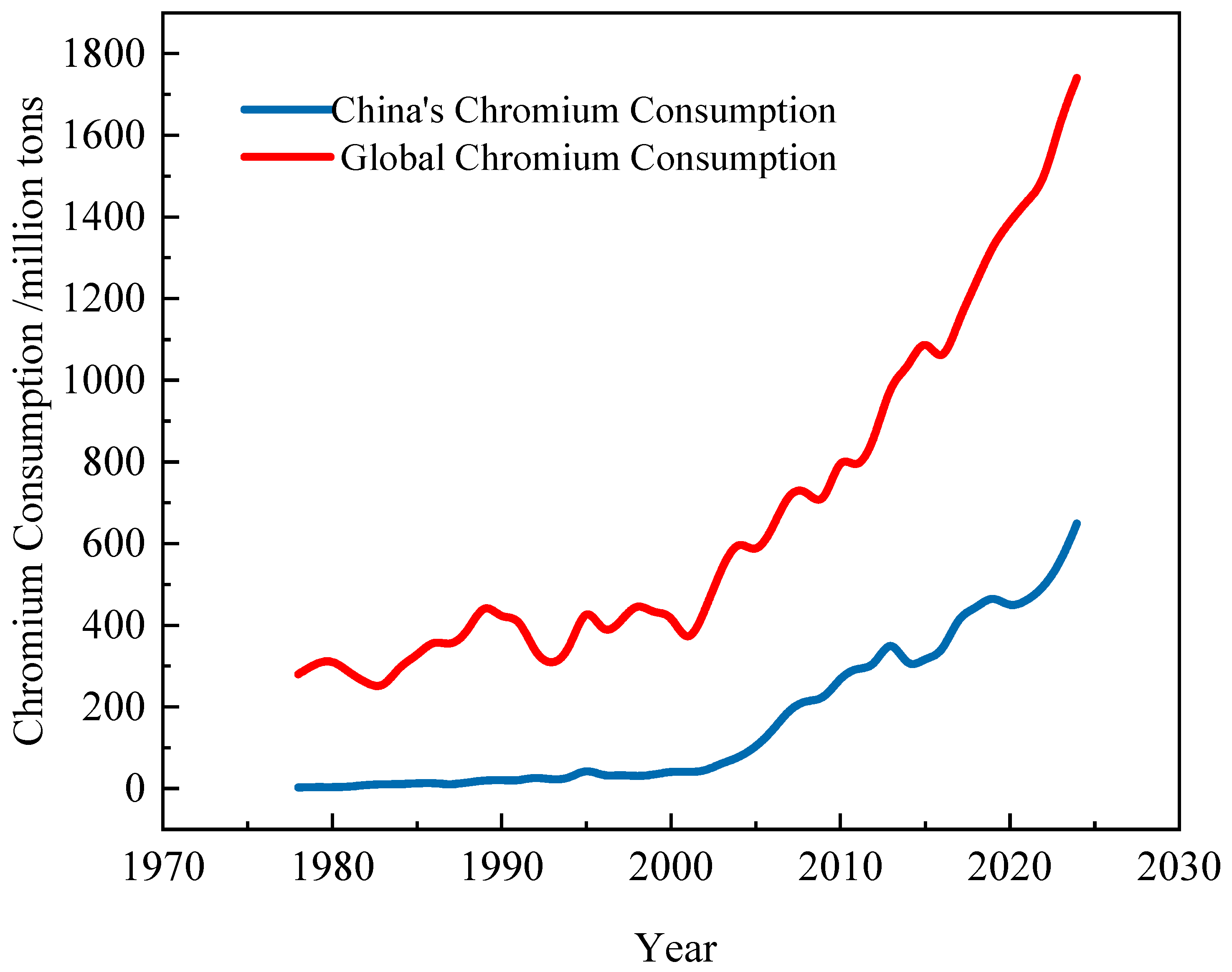
From 1981 to 2024, global and Chinese chromium consumption exhibited significant phased evolutionary characteristics (see Figure 2), and China’s position within the global chromium consumption framework also changed noticeably. Analyzing the global chromium consumption trend, it can be divided into two phases: the first phase from 1981 to 2000, during which global apparent chromium consumption rose from 2.8247 million tons to 4.3209 million tons, showing a trend of slow growth amidst fluctuations; the second phase began in 2001, characterized by rapid growth, with global apparent chromium consumption increasing from 3.4158 million tons to 17.3971 million tons, representing an average annual growth rate of 8.9%. This phase has been significantly driven by China’s rapid economic development, the expansion of the stainless steel industry, and accelerated industrialization and urbanization, greatly fueling the demand for global chromium resources. China’s chromium consumption trend aligns closely with the global chromium consumption trend, exhibiting strong growth momentum. Currently, China is the fastest-growing and largest consumer of chromium globally, achieving a transition in its position in the global chromium consumption market from being a ‘minor participant’ to a ‘core leader.’ From 1980 to 2000, China’s chromium consumption gradually increased, reaching merely 9% of global consumption by the year 2000. Since the new century, with the rapid development of the stainless steel industry, chromium consumption has surged from 403,200 tons in 2000 to 3.7637 million tons in 2013. In late 2014, influenced by the steel industry’s ‘capacity reduction’ policies and environmental pressures, consumption fell to 2.8739 million tons. Subsequently, stimulated by the upgrading of the stainless steel industry and the rising demand for high-purity metallic chromium in new energy and aerospace fields, chromium consumption continually increased, reaching a historical peak in 2019 of 35% of global chromium consumption. In 2020, chromium consumption experienced a decline due to the impact of the COVID-19 pandemic, but it slowly increased afterwards, reaching as high as 5.4917 million tons in 2023 after the pandemic restrictions were lifted, with an average annual growth rate of 12.32%. In 2024, chromium consumption further increased to 6.4743 million tons, accounting for 33.57% of the global total.

4. Prediction of Chromium Demand Based on Departmental Needs Method

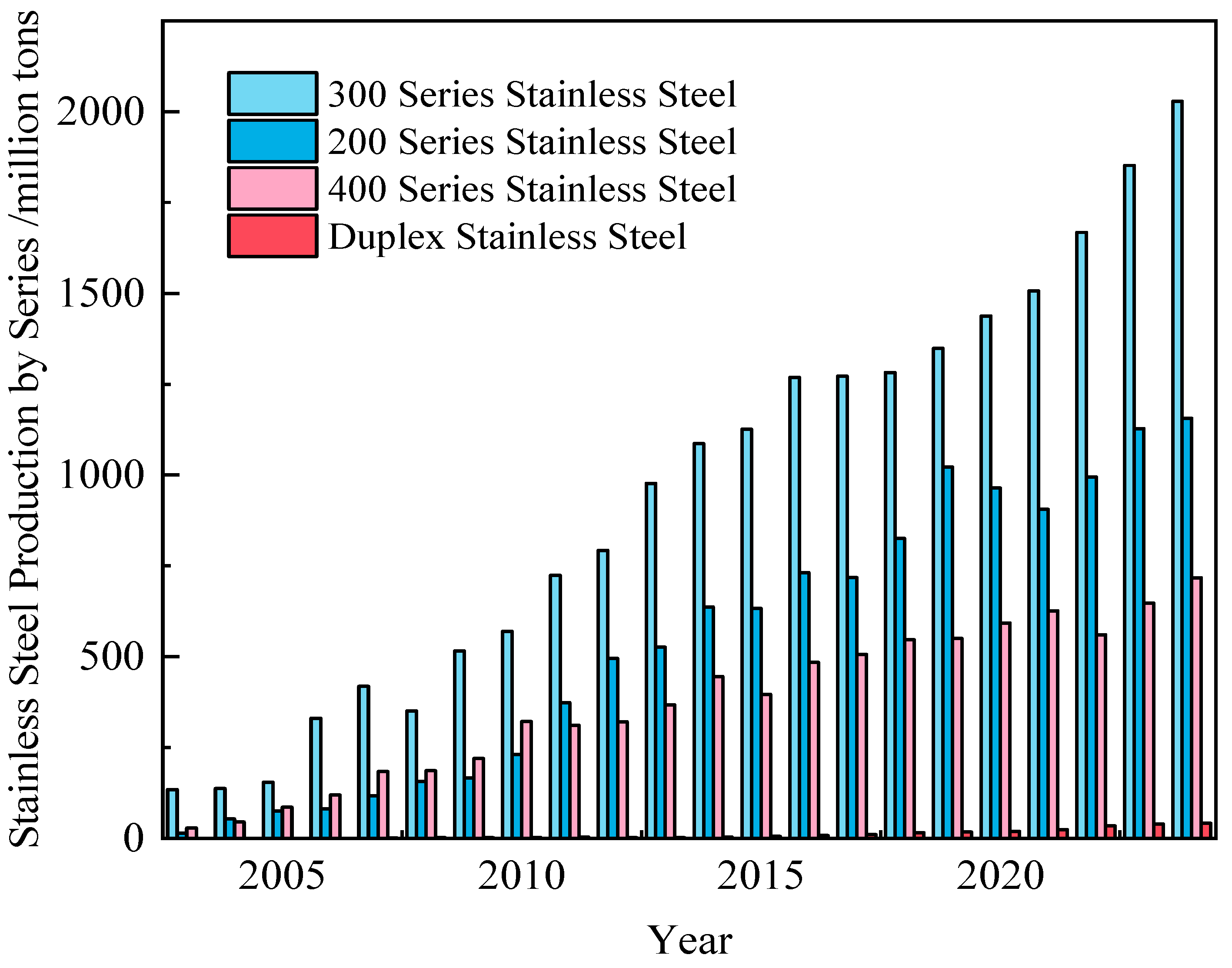
90% of chromium in China is used for the production of stainless steel, with 27.69% accounted for by 200 series of the stainless steel, 45.44% by 300 series, 15.8% by 400 series, and 1.07% by duplex stainless steel (see Figure 3).

4.1. Demand Forecast for the Chromium-Stainless Steel Sector

4.1.1. Prediction of 200 Series

According to the production data of 200 series stainless steel from 2005 to 2024, its output has shown significant fluctuations but an overall rapid growth trend. In 2005, China’s production of 200 series stainless steel was only 750,000 tons. Benefiting from accelerated urbanization and the rise in the home appliance industry, the market demand for the low-cost 200 series stainless steel was strong, which drove production to grow rapidly from 2005 to 2014. By 2014, production had increased to 6.37 million tons, with an average annual growth rate of 29.3%. In 2015, due to tightened environmental protection policies, production experienced negative growth for the first time. From 2016 to 2019, the industry gradually adapted to the environmental protection policies; although production resumed growth, the average annual growth rate decreased to 13.14%. The impact of the COVID-19 pandemic from 2020 to 2021 led to a decline in demand, resulting in a temporary drop in production to 9.058 million tons. From 2022 to 2024, with the rise in new demands such as new energy vehicles and photovoltaic brackets, there was a certain increase in demand, causing the production of 200 series stainless steel to grow from 9.95 million tons to 11.56 million tons, with a compound growth rate of 4.1%, which is significantly lower compared to the previous period.

The 200 series stainless steel belongs to the chromium-manganese-nitrogen stainless steel category, substituting part of the nickel with high manganese and nitrogen content to reduce production costs. It is characterized by its non-magnetic properties, high strength, and low price. However, it is necessary to maintain sufficient chromium content to preserve basic stainless properties [32], with chromium content typically ranging from 15% to 19%. This material is primarily used in construction, home appliances, and industrial equipment. However, as the growth rate in the construction industry slows and the home appliance market gradually saturates, traditional demand is growing slowly. Although emerging sectors such as new energy vehicles and photovoltaic brackets are driving an increase in stainless steel demand, the 200 series struggles to enter the mid-to-high-end market due to its performance limitations. The “National Economic and Social Development Plan” released in 2023 mentions accelerating the transformation and upgrading of key industries and continuously consolidating the achievements in resolving excess steel production capacity. The energy-saving and carbon-reduction transformations in key industries such as steel and petrochemicals are steadily advancing. This series of policy directions will impact the production of 200 series stainless steel, promoting the industry’s development towards transformation, upgrading, energy savings, and carbon reduction, thereby indirectly affecting the 200 series stainless steel market. Moreover, developed countries like the United States and Japan have long since replaced all 200 series stainless steel water pipes with 300 series stainless steel as early as 1993. Therefore, it is anticipated that the production of the 200 series stainless steel in China will gradually decline and may even be entirely replaced, inevitably leading to a decrease in the demand for chromium in the future.

An in-depth analysis of the production and growth rate of China’s 200 series from 2005 to 2024 indicates, through trend analysis and parameter adjustments, that the future production of China’s 200 series will reach 11.78 million tons in 2025, 11.65 million tons in 2030, 8.67 million tons in 2035, and 2 million tons in 2040, significantly reducing the demand for chromium.

4.1.2. Prediction of 300 Series

Based on the production data of the 300 series from 2005 to 2024, the development of 300 series production exhibits the characteristics of a “high-speed growth—adjustment and optimization—stable recovery” phase. In 2005, the production of 300 series stainless steel in China was only 1.5492 million tons. By 2015, due to the vigorous development of the real estate industry, the implementation of the home appliance subsidy policy, and the booming construction and decoration industry, the market demand for 300 series stainless steel surged, leading to an increase in production to 11.12654 million tons, with an average annual compound growth rate of 16.5%, marking the high-speed growth period. From 2016 to 2020, affected by global nickel price fluctuations and domestic environmental production restrictions, the industry entered a deep adjustment period, and the production growth rate slowed down to an average annual rate of 7.2%. From 2021 to 2024, driven by the demand for new energy equipment and high-end chemical equipment, along with the promotion of green manufacturing technology upgrades by the “dual carbon” policy, the competitiveness of 300 series stainless steel has been further enhanced, resulting in a stable recovery in production, with the average annual growth rate rising to 8.5%. By 2024, production is expected to reach 20.2914 million tons, accounting for 52% of China’s total stainless steel output.

The 300 series, as the core category of austenitic stainless steel, has a typical composition of 18% chromium and 8% nickel. With its excellent corrosion resistance, weldability, and formability, it has long occupied a dominant position in the total output of stainless steel. The 300 series is primarily utilized in heavy industry, light industry, consumer goods, and construction and decoration. Among these, its application in food contact materials is particularly notable. As the national economy transitions towards high-quality development, the demand for 300 series is expected to continue to grow. However, the growth model is undergoing significant changes; in traditional sectors, the real estate industry is shifting from rapid expansion to stable development, while household appliances are gradually entering a renewal phase, resulting in a tendency for demand growth to moderate. Conversely, in the high-end manufacturing sector, the demand for 300 series is poised for rapid growth in products such as electric vehicle battery casings, charging station equipment, and photovoltaic inverters. Additionally, with a heightened awareness of environmental protection and the widespread acceptance of sustainable development concepts, industries like chemicals and energy are increasingly demanding greater corrosion resistance and longevity from equipment, further expanding the application scope of the 300 series. Nevertheless, from a long-term perspective, the market is gradually becoming saturated due to the expansion of 300 series production capacity, intensifying industry competition, significant price fluctuations of key alloying elements like nickel and chromium, and the emergence of new materials that may replace it.

Based on the above analysis and in conjunction with the historical production and growth rate of 300 series, using trend analysis and parameter adjustment, it is predicted that China’s production of 300 series stainless steel will reach 21.5088 million tons by 2025, 28.5121 million tons by 2030, 33.0378 million tons by 2035, and 33.8721 million tons by 2040. As the primary consumption sector of chromium, the growth trend of 300 series stainless steel production will directly impact the future demand pattern for chromium in China.

4.1.3. Prediction for 400 Series

According to the production data of the 400 series from 2005 to 2024, there is a significant growth trend, with production increasing from 860,000 tons in 2005 to 9.8 million tons in 2024, resulting in an average annual compound growth rate of 16.9%. The historical development trend can be divided into three phases: from 2005 to 2010, benefiting from the expansion of traditional industries such as domestic machinery manufacturing and auto parts, production grew at a high average annual growth rate of 18.7%; from 2011 to 2018, affected by factors such as steel industry overcapacity and environmental protection policies, the annual growth rate slowed to 8.2%; from 2019 to 2024, driven by the rapid rise in the new energy vehicle industry and the upgrading transformation of the home appliance sector, production experienced a new round of growth, with the average annual growth rate rising to 14.5%.

The 400 series belongs to the ferritic and martensitic stainless steel categories, primarily composed of 12–18% chromium as the main metallic element, with little to no nickel content. It exhibits characteristics such as high strength, high hardness, resistance to high temperatures, and oxidation resistance, making it widely applicable in fields such as home appliances, kitchen and bathroom accessories, automotive exhaust systems, and hardware products. With advancements in technology and reductions in costs, the 400 series is gradually penetrating high-end sectors such as automotive manufacturing, nuclear power equipment, and high-pressure hydrogen storage containers. As the ‘Made in China 2025’ strategy progresses, the demand for lightweight, high-strength, and heat-resistant components in the automotive sector continues to increase. The 400 series, due to its superior properties, is seeing an expanding application in automotive exhaust systems. Meanwhile, in the home appliance industry, there is a growing demand for the 400 series stainless steel to enhance product quality. However, the corrosion resistance of 400 series stainless steel is somewhat inferior to that of the 300 series stainless steel, which limits its applications in areas with high corrosion resistance requirements.

Taking into account the above factors, and combining an analysis of the historical output and growth rate of 400 series stainless steel, parameter optimization and trend analysis have led to the conclusion that China’s production of 200 series stainless steel is projected to reach 7.107 million tons by 2025, 8.5419 million tons by 2030, 10.2608 million tons by 2035, and 12.4356 million tons by 2040. As the output of 400 series stainless steel changes, the demand for chromium will also show a corresponding increase, although the growth rate will gradually slow down as production increases.

4.1.4. Prediction of Duplex Stainless Steel

According to statistical data from 2005 to 2024, the development of duplex stainless steel production has shown a significant characteristic of ‘slow at first, then rapid’. In 2005, China produced only 828 tons of duplex stainless steel, and early growth was relatively slow due to limitations such as technological levels. However, with continuous breakthroughs in stainless steel production technology and the rapid development of high-end equipment manufacturing, production began to accelerate, reaching 411,600 tons by 2024, with a compound annual growth rate of 44.94%. Although it only accounts for 1.7% of the total stainless steel production, it possesses strong development potential.

Duplex stainless steel is a special type of stainless steel composed of austenite and ferrite, with a chromium content of 22–25%. It also contains a certain amount of molybdenum and nitrogen, providing high strength, excellent resistance to stress corrosion, and good weldability. It is widely used in high-end fields such as chemical pipelines, papermaking machinery, seawater desalination, and energy. With the introduction of the ‘dual carbon’ goals and the government’s strong support for high-end manufacturing, the new energy industry is booming, leading to a strong demand for high-performance corrosion-resistant materials, which in turn has increased the demand for duplex stainless steel. Furthermore, the government has increased investment in the R&D of stainless steel materials, driving continuous innovation in duplex stainless steel production, lowering production costs, and improving production efficiency, further enhancing its market competitiveness. However, the production process of duplex stainless steel is complex, with high requirements for production equipment and technology, resulting in elevated production costs. In some traditional sectors, users lack sufficient understanding of its properties, which limits the further expansion of duplex stainless steel.

Based on the analysis of historical production and growth rates of duplex stainless steel, along with the trends in production, it is projected that the future production of duplex stainless steel in China will reach 598,700 tons by 2025, 1,164,600 tons by 2030, 2,013,100 tons by 2035, and 3,201,700 tons by 2040. Given the high chromium content in duplex stainless steel, the rapid increase in its production will lead to a stronger demand for chromium in the future, becoming a significant driving force behind the demand for chromium in our country.

4.2. Chromium Demand Forecast

Over 90% of China’s chromium consumption is directed towards stainless steel production. The rapid expansion of stainless steel manufacturing commenced in 2000, coinciding with the onset of chromium’s accelerated growth phase. Consequently, data analysis was conducted on China’s stainless steel output and chromium consumption from 2000 to 2024. Results reveal a pronounced linear correlation between stainless steel output and chromium consumption (see Figure 4), yielding the linear equation W = 0.13188 * V + 65.93112 (where W denotes chromium demand and V represents total stainless steel production).

The model’s fitting quality is assessed through three core metrics: the coefficient of determination (R²), Pearson’s correlation coefficient, and root mean square error(RMSE). The coefficient of determination R² was 0.9533 (values closer to 1 indicate superior fit quality), confirming a significant linear relationship between stainless steel output and chromium consumption with high overall linear fitting accuracy. The Pearson correlation coefficient quantifies the strength of linear association between two variables. The correlation coefficient between stainless steel output and chromium consumption stands at 0.98 (where values closer to 1 indicate a stronger correlation), demonstrating a robust positive linear relationship. The root mean square error (RMSE) of 362,700 tons remains at a low level overall, indicating controllable fluctuation deviations in the fitting results. This further validates the reliability of their linear relationship, providing robust data support for forecasting chromium demand based on stainless steel production.

Error Analysis: In practical terms, chromium resource consumption is influenced not only by stainless steel production volumes but also by factors such as stainless steel product composition, chromium resource recovery rates, and short-term policy interventions. This study employed linear regression with ‘total stainless steel production’ as the sole independent variable, omitting these granular factors. Consequently, certain chromium consumption data deviated from the fitted line, generating errors.

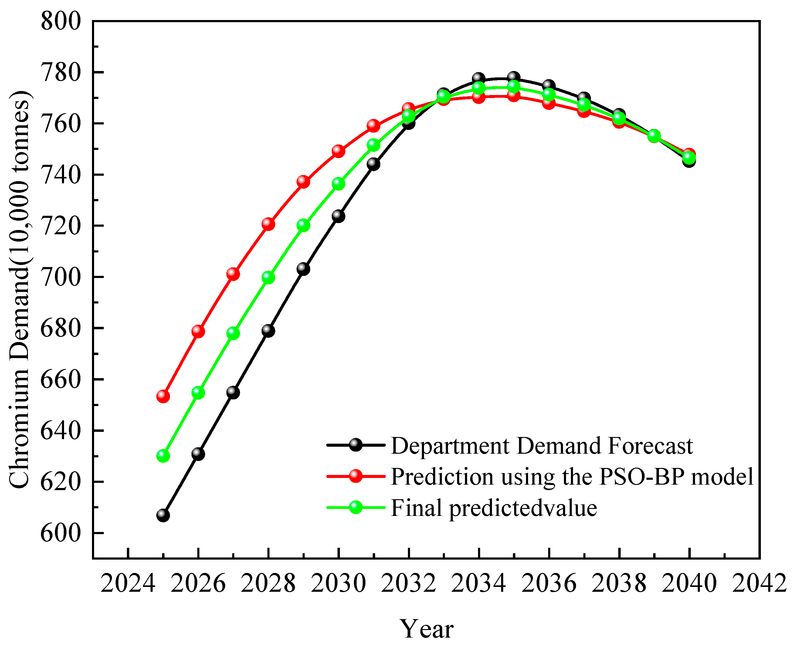
In summary, based on the four stainless steel product series identified, the total stainless steel production volume is projected as follows: 41.0038 million tons in 2025, 49.8732 million tons in 2030, 53.9774 million tons in 2035, and 51.5099 million tons in 2040. Consequently, China’s chromium demand is projected as follows: 6.0669 million tons in 2025, 7.2366 million tons in 2030, 7.7779 million tons in 2035, and 7.4524 million tons in 2040.

5. Chromium Demand Prediction Based on PSO-BP Neural Network Model

5.1. Chromium Gray Correlation Analysis

In order to further validate the feasibility of the driving variables for chrome demand forecasting, statistical methods were employed to quantitatively test the data of the five influencing factors mentioned above. This paper utilizes the gray correlation analysis method. The principle is to determine the degree of association between two factors based on the similarity of their trends over time. The closer the trends are, the higher the degree of association; conversely, the lower the degree of association [33]. The results of the correlation coefficient calculations are listed in

Table 1. Relevance Results.

Evaluation Item	Relevance	Ranking
Gross Domestic Product of the Secondary Sector	0.969	1
Gross Domestic Product	0.966	2
Stainless Steel Production	0.915	3
Urbanization rate	0.843	4
Population	0.842	5

.

The ranking of the driving variables that influence the prediction of chromium demand in China, from most to least significant, is as follows: GDP, Output of secondary industry, stainless steel production, urbanization rate, and population. The correlation coefficients for these variables are all greater than 0.8, indicating that these variables have a strong impact on the demand for chromium in China. Therefore, selecting these five variables as the primary driving factors for predicting chromium demand in China is reasonable.

5.2. PSO-BP Neural Network Model Construction

5.2.1. Parameter Setting and Data Preprocessing

A PSO-BP model is constructed using MATLAB R2024a, where relevant parameters need to be set during model construction. Firstly, the network structure of the neural network is determined, specifying the number of nodes in the input layer, hidden layer, and output layer. In this study, five influencing factors are selected as input values, including stainless steel output, urbanization rate, population, value added of the secondary industry, and GDP, resulting in an input layer node count of 5. The optimal number of nodes in the hidden layer is determined to be 7 using the trial-and-error method, while the output value, representing chromium demand, leads to 1 output layer node. The maximum number of iterations for the BP neural network is set to 50. The learning rate for the neural network is set to 0.01, with the activation function as tansig, training occurring over 1000 iterations, and the training goal set at 0.000001. The parameters for the particle swarm optimization (PSO) algorithm are also set: population size is 10, weight coefficients c1 = c2 = 2, constraint factor r = 0.9, and iteration count set to 50, with an inertia weight ω = 0.9, maximum particle velocity Vmax = 3, and minimum velocity Vmin = -3. The fitness function employed is the root mean square error ($RMSE$) between the predicted values of the BP neural network and the actual values.

Collect data on China’s chromium consumption, stainless steel production, urbanization rate, population, value of the secondary industry, and factors affecting GDP from 1981 to 2024. During the training process, to improve predictive accuracy, representative data samples will be selected, and the more data in each group, the better. As different variables may have different magnitudes and units, normalization of the input data will be performed to eliminate dimensional influence and accelerate network convergence, using the following formula:

$$x_n={\displaystyle \frac{x-\min (X)}{\max (X)-\min (X)}}$$

(5)

where $x_n$ is the normalized value, $x$ is the value of a sample in the original data on that feature, $X$ is the set of all sample values of that feature in the training data set, $\min (X)$ is the minimum value of that feature in the training set, and $\max (X)$ is the maximum value of that feature in the training set.

This article selects 44 data sets as shown in

Table 2. China’s Population, Urbanization Rate, Secondary Industry Output Value, Stainless Steel Production, GDP Input Value and Chromium Consumption Output Value from 1978 to 2024.

Population per 10,000	Urbanization Rate %	Secondary Industry Output Value/Ten Thousand Yuan	Stainless Steel Production/10,000 tons	China’s GDP per 10,000 Yuan	Chromium Consumption/10,000 tons
100,072.00	20.16	2269.00	23.48	4935.80	2.45
101,654.00	21.13	2397.60	23.65	5373.40	6.84
103,008.00	21.62	2663.00	23.83	6020.90	9.30
104,357.00	23.01	3124.70	24.00	7278.50	8.58
105,851.00	23.71	3886.40	19.00	9098.90	11.15
107,507.00	24.52	4515.10	20.14	10376.20	11.78
109,300.00	25.32	5273.80	21.35	12,174.60	7.05
111,026.00	25.81	6607.20	22.64	15,180.40	13.14
112,704.00	26.21	7300.70	24.00	17,179.70	18.22
114,333.00	26.41	774.10	16.40	18,872.90	19.54
115,823.00	26.37	9129.60	20.50	22,005.60	16.59
117,171.00	27.63	11,725.00	25.80	27,194.50	27.35
118,517.00	28.14	16,472.70	21.20	35,673.20	18.71
119,850.00	28.62	22,452.50	26.00	48,637.50	21.50
121,121.00	29.04	28,676.70	32.44	61,339.90	48.16
122,389.00	29.37	33,827.30	31.34	71,813.60	27.21
123,626.00	29.92	37,545.00	33.22	79,715.00	32.35
124,761.00	30.40	39,017.50	28.44	85,195.50	27.92
125,786.00	30.89	41,079.90	30.22	90,564.40	31.60
126,743.00	36.22	45,663.70	60.00	100,280.10	40.32
127,627.00	37.70	49,659.40	73.00	110,863.10	38.51
128,453.00	39.10	54,104.10	114.00	121,717.40	39.87
129,227.00	40.53	62,695.80	177.80	137,422.00	60.15
129,988.00	41.80	74,285.00	236.40	161,840.20	73.14
130,756.00	43.00	88,082.20	316.00	187,318.90	99.11
131,448.00	43.90	104,359.20	530.00	219,438.50	138.85
132,129.00	44.90	126,630.50	720.60	270,092.30	192.88
132,802.00	45.70	149,952.90	694.30	319,244.60	215.76
133,450.00	46.60	160,168.80	880.47	348,517.70	213.18
134,091.00	49.70	191,626.50	1125.60	412,119.30	271.39
134,916.00	51.30	227,035.10	1409.10	487,940.20	295.37
135,922.00	52.60	244,639.10	1608.70	538,580.00	290.89
136,726.00	53.73	261,951.60	1898.40	592,963.20	376.37
137,646.00	54.77	277,282.80	2169.20	643,563.10	287.39
138,326.00	56.10	281,338.90	2156.20	688,858.20	318.40
139,232.00	57.35	295,427.80	2493.78	746,395.10	324.17
140,011.00	58.52	331,580.50	2577.37	832,035.90	424.16
140,541.00	59.58	364,835.20	2670.68	919,281.10	437.93
141,008.00	60.60	380,670.60	2940.00	986,515.20	474.82
141,212.00	63.90	383,562.40	3013.90	1,013,567.00	440.73
141,253.00	64.72	451,544.10	3063.20	1,149,237.00	456.87
141,256.00	65.22	473,789.90	3197.50	1,204,724.00	488.93
141,223.00	66.16	482,588.50	3667.59	1,260,582.10	549.17
141,144.00	67.00	492,087.00	3944.11	1,349,084.00	647.70

Data source: National Bureau of Statistics of China; USGS.

, dividing the processed sample data into a training set and a testing set, with 34 sets serving as training samples and 10 sets as testing samples. This partitioning ensures an adequate number of training samples, effectively avoiding the potential overfitting caused by “short-term sample limitations”, with all gray correlation coefficients exceeding 0.8. All training data in this study originates from authoritative institutions such as the USGS and the National Bureau of Statistics, thereby minimizing random errors and statistical biases. After the model has made predictions, the results are then re-normalized to obtain the actual predicted value of chromium resource demand.

5.2.2. Model Training and Evaluation

In order to further compare the performance differences among models and evaluate the predictive effects of the models, both the traditional BP neural network and the particle swarm optimized BP neural network are selected for prediction. The performance evaluation indicators employed are the Mean Absolute Error ($MAE$), Root Mean Square Error ($RMSE$), and the Coefficient of Determination ($R^2$). A smaller Mean Absolute Error and a larger Coefficient of Determination indicate better predictive performance of the model. The calculation formulas are as follows:

$$MAE={\displaystyle \frac{1}{N}}{\displaystyle \sum _{i=1}^N\left|x_i-x_i^{*}\right|}$$

(6)

$$RMSE=\sqrt{{\displaystyle \frac{{\displaystyle {\sum }_{i=1}^N{(x_i-x_i^{*})}^2}}{N}}}$$

(7)

$$R^2={\displaystyle \frac{({\displaystyle {\sum }_{i=1}^N(x_i-\overline{x})(x_i-\overline{x}){)}^2}}{{\displaystyle {\sum }_{i=1}^N{(x_i-\overline{x})}^2•{\displaystyle {\sum }_{i=1}^N{(x_i-\overline{x})}^2}}}}$$

(8)

5.2.3. Model Comparison and Analysis Prediction

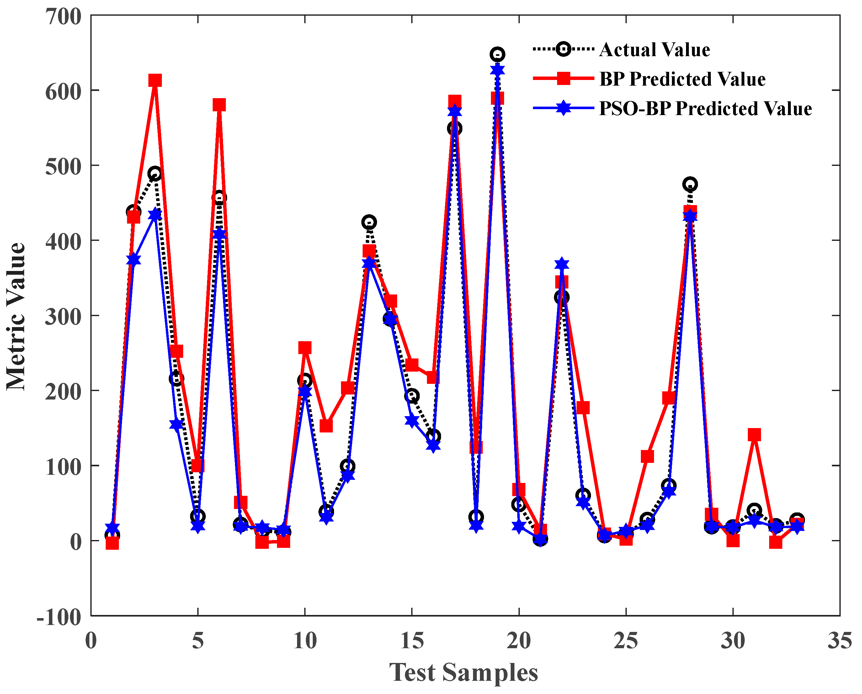
Based on the parameter settings established from the above model, a traditional BP neural network model and a PSO-BP neural network model were constructed, and 34 test samples were selected for prediction, as shown in Figure 5. It can be seen from Figure 5 that the BP prediction model has a relatively large error. After optimization through the PSO algorithm, the PSO-BP prediction model aligns more closely with the measured values, indicating that the PSO-BP prediction model has better fitting performance and generalization ability, reflecting the relative superiority of the optimization algorithm.

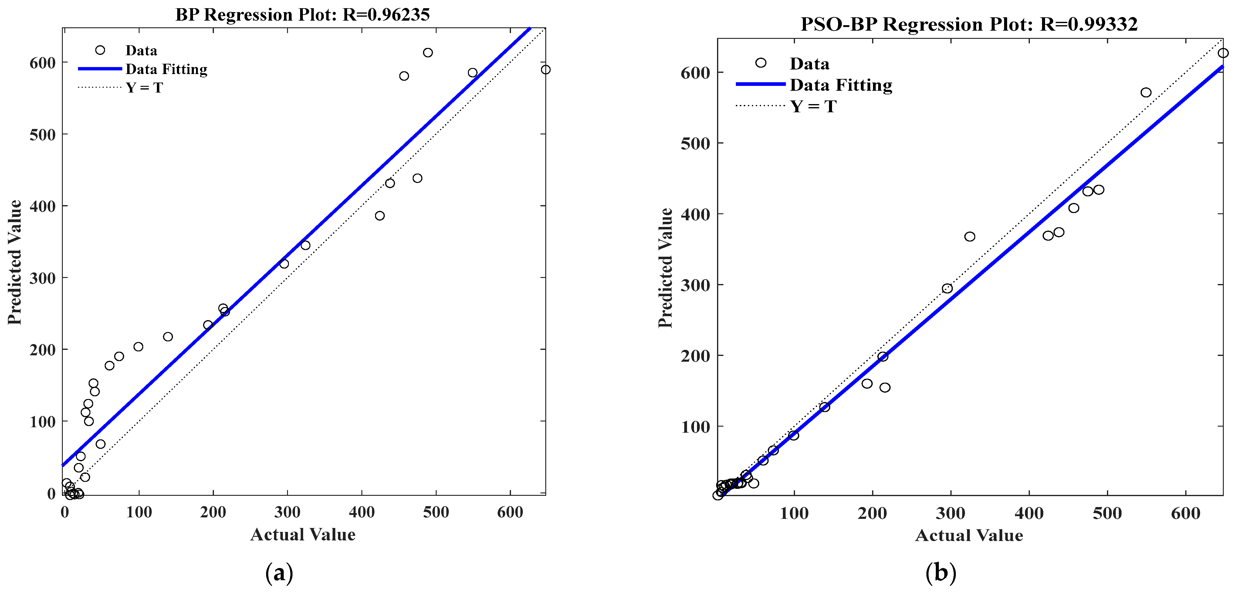
To predict the performance of the two models, the correlation coefficient curve between the measured values and predicted values of the validation data is shown in Figure 6. As can be seen from Figure 6, the PSO-BP prediction model has a good regression fit, with a correlation coefficient reaching 0.99332, while the traditional BP prediction model has a correlation coefficient of 0.96235. This indicates that the PSO-BP model has a higher degree of fit, demonstrating a strong alignment between the measured values and predicted values.

For the prediction results of the two models, a comparative analysis was conducted using the model evaluation metrics as per Formulas (6), (7), and (8), as shown in

Table 3. Performance Analysis of Two Neural Network Models.

Model	Mean Absolute Error ($\mathit{M}\mathit{S}\mathit{E}$)	Root Mean Square ($\mathit{R}\mathit{M}\mathit{S}\mathit{E}$)	Coefficient of Determination (${\mathit{R}}^2$)
BP	22.3839	34.1638	0.9577
PSO-BP	14.5382	21.5566	0.9880

. Compared to the traditional BP neural network prediction model, the PSO-BP model exhibits higher prediction accuracy.

5.2.4. PSO-BP Model Prediction Results

Forecast results indicate that China’s chromium demand will peak in 2035. In 2025, the demand for chromium is projected to be 6.5322 million tons, increasing to 7.4905 million tons in 2030, reaching its peak at 7.7095 million tons in 2035, and then decreasing to 7.4776 million tons by 2040.

6. Analysis of the Forecast Results

6.1. Prediction Results

The predicted results of the two methods are summarized in Figure 7. Considering the current consumption status, China’s chromium demand is projected to be 6.2996 million tons in 2025, 7.3635 million tons in 2030, 7.7437 million tons in 2035, and 7.465 million tons in 2040. The subsequent development trend of chromium demand can be roughly divided into two stages: from 2024 to 2035, chromium demand will continue to increase with an average annual growth rate of 2.1%. In 2035, China’s chromium demand will peak at 7.3299 million tons. From 2035 to 2040, demand will decline slightly due to the restructuring of the stainless steel industry and the saturation of stainless steel products, but the rate of decline will be relatively slow, at a decrease of 0.7%.

6.2. Robustness Analysis of Prediction Results

To validate the robustness of the forecast results, this paper employs a rolling time window verification method to assess the reliability and robustness of the predictions generated by the two aforementioned approaches.

6.2.1. Methodology

The rolling time window validation method reconstructs predictive models by partitioning historical data into training and testing sets with varying starting years [34,35]. It compares the ‘prediction-actual value deviation’ and ‘consistency of windowed predictions’ across different time windows. If error fluctuations are minimal and deviations at critical nodes remain manageable, this indicates the model exhibits low dependency on data samples and high robustness [36].

Based on the historical analysis of global and Chinese chromium consumption in Section 3 of this paper, the 44 sets of sample data were divided into three mutually exclusive and representative rolling windows, as shown in

Table 4. Division of Rolling Windows.

Window Number	Training Set Time Range	Test Set Time Range	Target Prediction Period
1	1981–2014	2015–2019	2020–2024
2	1981–2016	2017–2021	2022–2024
3	1981–2018	2019–2023	2024

. The department demand forecasting method employed only stainless steel production volume and chromium demand, while the PSO-BP approach utilized five driving variables alongside chromium demand.

6.2.2. Validation Steps

(1)

Model Reconstruction

Based on the window training set data, the two forecasting methods were reconstructed separately:

① Department Demand Forecasting Method: For each window training set, the linear relationship between “stainless steel output and chromium demand” was recalculated. Combined with the actual stainless steel output from 2015 to 2024, the predicted chromium demand values for the target period were output for each window.

② PSO-BP Neural Network Model: In accordance with the parameter settings specified in Section 5.2.1, the model was retrained using the “driving variables–chromium demand” data samples from each window training set, and the predicted chromium demand values for the target prediction period were output.

(2)

Error Metric Calculation

For the prediction results of each window, the same error evaluation metrics (MAE and RMSE) as those in Section 5.2.2 were adopted to compare the deviations between the predicted values and the actual chromium demand values from 2015 to 2024.

(3)

Inter-window Consistency Test

The Coefficient of Variation (CV) of the prediction results from the 3 windows was calculated (CV = Standard Deviation of Samples/Mean of Samples) [37]. If CV ≤ 10%, it indicates that the fluctuations in results across different windows are small. Meanwhile, for the year 2024 (included in all 3 windows), the deviations between the predicted values and the actual values reported in the original study were compared to verify the consistency of the conclusions.

6.2.3. Validation Results and Analysis

(1)

Prediction Error Results

The error metrics of the 3 rolling windows are presented in

Table 5. Statistical Results of Error Indicators for Each Window.

Window Number	Department Demand Forecasting Method		PSO-BP Neural Network Model		Inter-Window Coefficient of Variation (CV%)
	MAE (10,000 tons)	RMSE (10,000 tons)	MAE (10,000 tons)	RMSE (10,000 tons)
1	18.26	23.51	12.89	16.73	8.2
2	16.94	21.87	11.56	15.29	7.5
3	15.78	19.63	10.32	13.85	6.9
Mean Value	17	21.67	11.59	15.29	-

below. The MAE and RMSE values of both forecasting methods remain at low levels, and the maximum inter-window CV is 8.2%, which is lower than the 10% robustness threshold. This indicates that the models exhibit strong adaptability to different sample intervals, with no significant overfitting or underfitting issues.

(2)

Consistency Check

Taking the actual values in 2024 as the core verification node, the deviations of each window from the original text are all ≤2.27%, as shown in

Table 6. Predicted Values of Each Window in 2024 and Their Deviations from the Actual Values.

Forecasting Method	Window 1 Prediction (10,000 tons)	Window 2 Prediction (10,000 tons)	Window 3 Prediction (10,000 tons)	Deviation from Actual Value (%)
Department Demand Forecasting Method	662.15	655.82	649.37	2.27–0.61
PSO-BP Model	658.37	651.29	648.15	1.70–0.11

. Moreover, all windows predict that the value will peak in 2035 and decrease after 2035, which is consistent with the trend of the prediction result analysis in Section 6.1 of the original text.

6.2.4. Robustness Conclusions

Results of the rolling time window verification indicate that the two forecasting methods exhibit small error fluctuations across different data windows (with a coefficient of variation (CV) ≤ 8.2%) and are insensitive to changes in the sample interval, demonstrating reliable model robustness. Additionally, the deviations between the 2024 predicted values and the actual values in the original text are ≤2.27%, and the demand trend (peaking in 2035 followed by a decline) is consistent. These findings further support the validity and credibility of the “Chromium Demand Forecast Results for 2025–2040” presented in Section 6.1 of the original text.

7. Conclusions

(1)

The forecasting results of the Department Demand Forecasting Method and the PSO-BP Neural Network Model indicate that China’s chromium demand will continue to grow in the next decade. This trend is consistent with existing studies to a certain extent, yet differences also exist. Zheng Minggui [23] applied a gray neural network to predict that China’s chromium demand would keep growing from 2020 to 2030, but did not predict chromium demand beyond 2030. This study conducts medium- and long-term forecasting of chromium demand: the average annual growth rate of chromium demand will drop to 2.1% during 2025–2035; China’s chromium demand will reach 7.7437 million tons in 2035, entering the peak period of chromium consumption; after 2035, affected by the industrial structure upgrading of the stainless steel industry and market saturation, the demand will decrease at an average annual rate of 0.7%. Therefore, China’s chromium demand presents a trend of slow growth followed by a slow decline after reaching the peak. Combined with the consistent results of the two forecasting methods, this study integrates qualitative and quantitative approaches to achieve more accurate predictions. The predicted chromium demand values are 6.2996 million tons in 2025, 7.3635 million tons in 2030, 7.7437 million tons in 2035, and 7.4650 million tons in 2040, respectively.

(2)

The upgrade of stainless steel products is the primary driving force that directly impacts chromium demand. The 300 series (with a chromium content of 18%) is the mainstay of demand, with a production amount reaching 33.8721 million tons by 2040, thus supporting long-term chromium consumption. Under policy influence, the production of the 200 series stainless steel (with a chromium content of 15%) is reduced to 2.0005 million tons by 2024, significantly decreasing its dependence on chromium. Conversely, duplex stainless steel (with a chromium content of 22%) is experiencing explosive growth in the new energy equipment sector, while demand in certain traditional sectors is dwindling.

(3)

By incorporating driving variables such as gross domestic product, urbanization rate, and total value of the secondary industry, and optimizing the weights of the BP neural network using particle swarm optimization, the model’s error has significantly decreased, with the RMSE dropping from 34.1638 to 21.5566 and the R2 rising from 0.9577 to 0.9880, This is consistent with the PSO-BP applied by Wang et al. [17] in forecasting for new energy vehicles, which further verifies the effectiveness of the particle swarm optimization (PSO) algorithm in improving the accuracy of the BP neural network.

References

1. Zeng, X.; Yuan, C.; Xu, H.; Han, J.; Tian, Y. Research on the situation of China’s chromium resource industry and its related strategies. Resour. Ind. 2015, 17, 39–44. [Google Scholar] [CrossRef]
2. Liu, X.; Chen, Q.; Zhang, Y.; Gao, T.M. Analysis of China’s chromium demand forecast and resource supply security situation. Resour. Sci. 2015, 37, 933–943. [Google Scholar]
3. Lu, Z. Analysis of the supply situation of chrome ore in China country and suggestions for guarantees. Metall. Econ. Manag. 2024, 2, 28–30. [Google Scholar]
4. Zeng, X.; Yuan, C.; Xu, H.; Han, J.; Tian, Y. Current status and investment suggestions for chromium ore development in the world. China Min. 2015, 24, 16–22. [Google Scholar] [CrossRef]
5. Zhang, Z.; Pan, Z.; Che, D.; Yan, Q.; Wu, Q. Characteristics of chromium ore resources in China and analysis of chromium supply and demand situation from 2021 to 2035. China Geol. 2024, 51, 1191–1209. [Google Scholar]
6. Liu, Q.; Sha, J.; Yan, J.; Zhang, G.; Fan, S.; He, G. Risk assessment and countermeasures of chromium resource supply in China. Resour. Sci. 2018, 40, 516–525. [Google Scholar]
7. Pan, Z.; Zhang, Z.; Wang, X.; Yang, Y.; Zhang, Z. Analysis of the current situation and future trend of recycled chromium resources in China. China Min. 2018, 27, 17–21. [Google Scholar]
8. Lü, P.; Gao, Y.; Zhang, Y.; Zhang, D. Kazakhstan chromite resource endowment, supply pattern and China–Kazakhstan production capacity cooperation suggestions. Northwest Geol. 2022, 55, 297–305. [Google Scholar] [CrossRef]
9. Zhao, P. The stainless steel industry explores new development paths. China Metall. News 2025, 003. [Google Scholar] [CrossRef]
10. Li, M.; Kong, Y. Natural gas price forecasting based on time series model. Oil Gas New Energy 2023, 35, 61–66. [Google Scholar] [CrossRef]
11. Li, H.; Liu, Q.; Chen, Y.; Han, M.; Wu, X. Forecast and analysis of China’s natural gas demand trend. Nat. Gas Technol. Econ. 2025, 19, 82. [Google Scholar]
12. Li, R.; Jin, L.; Sun, L.; Zhao, J.; Chen, S.; Zheng, L. Forecasting the development trend of big data algorithms in China’s petroleum and petrochemical field based on time series statistical method. Oil Drill. Prod. Technol. 2024, 46, 525–548. [Google Scholar] [CrossRef]
13. Shi, Y.; Peng, B. Forecasting coal throughput of Ningbo Port based on GM (1,1) and KPCA-GA-BP. Shipp. Manag. 2024, 46, 6–10+43. [Google Scholar] [CrossRef]
14. Chen, Z.; Zhu, Q.; Zou, X.; Wu, H.; Xing, K.; Tang, X. Research on the development trend of nickel resource industry chain under the “Dual Carbon” background. China Min. Mag. 2024, 33, 54–63. [Google Scholar] [CrossRef]
15. Yuan, W.; Zheng, M. Scenario analysis of China’s bauxite resource demand based on BP neural network. Resour. Ind. 2014, 16, 132–137. [Google Scholar] [CrossRef]
16. Gong, T.; Zheng, M. Scenario analysis of China’s copper mineral resource demand based on BP neural network. Nonferrous Met. Sci. Eng. 2014, 5, 99–106. [Google Scholar] [CrossRef]
17. Wang, X.; Hao, T.; Ma, C. Sales forecasting model of new energy vehicles based on PSO-BP neural network. Sci. Technol. Eng. 2024, 24, 13467–13474. [Google Scholar] [CrossRef]
18. Jiang, B.; Zhang, J.; Fu, J.; Ding, G.; Zhang, Y. Research on check-in baggage flow prediction for airport departure passengers based on improved PSO-BP neural network combination model. Aerospace 2024, 11, 953. [Google Scholar] [CrossRef]
19. Xiong, F.; Gong, X.; Qiu, T.; Xu, X.; Gui, W. Genesis of different types of minerals in pod-shaped chromite and their constraints on the mineralization process. Bull. Miner. Rock Geochem. 2025, 44, 1–16. [Google Scholar] [CrossRef]
20. Wang, X.; Liu, C.; Wang, A. Characteristics, supply-demand situation and enterprise competition of global chromium ore resource. China Min. 2025, 34, 449–457. [Google Scholar] [CrossRef]
21. Zhang, Z.; Zhang, Z.; Pan, Z.; Wu, Q.; Xu, H. Analysis of China’s supply safety by global chromium ore resource countries. China Min. 2019, 28, 69–76. [Google Scholar] [CrossRef]
22. Li, J.; Zhou, N.; Hu, P.; Wu, Y.; Cheng, J. Evolution of trade network pattern of chromium ore in global and analysis of competitiveness. China Min. 2024, 33, 48–58. [Google Scholar] [CrossRef]
23. Zheng, M.; Yuan, X. Forecast of China’s chrome ore demand from 2020 to 2030 based on a gray neural network. Resour. Dev. Mark. 2018, 34, 747–752. [Google Scholar] [CrossRef]
24. Zhang, W. Analysis and forecast of world chromium ore resource demand. Resour. Ind. 2016, 18, 87–91. [Google Scholar] [CrossRef]
25. Zheng, M.; Li, Q. Scenario prediction of China’s oil resource demand from 2020–2030. Adv. Earth Sci. 2020, 35, 286–296. [Google Scholar] [CrossRef]
26. Wu, Q.; Zhang, Z.; Pan, Z.; Zhang, Z.; Xu, H. Forecast of China’s vanadium resource demand from 2020 to 2035. China Min. 2021, 30, 48–56. [Google Scholar] [CrossRef]
27. Qiu, Q. Research on investor age prediction based on PSO-BP algorithm. Mod. Comput. 2024, 30, 61–65. [Google Scholar]
28. Zhou, P.; Ma, J.; Ma, Y.; Wang, N.; Liu, L.; Han, L. Water consumption model of transpiration based on BP neural network and particle swarm optimization algorithm. Ningxia Eng. Technol. 2025, 1–5. [Google Scholar]
29. Wang, J.; Chen, H.; Wang, L. Prediction of China’s silicon wafer price: A GA-PSO-BP model. Mathematics 2025, 13, 2453. [Google Scholar] [CrossRef]
30. Zhang, Z.; Zhou, W. Prediction of transpiration of reference crops based on PSO-BP neural network. Water-Sav. Irrig. 2014, 11, 87–90+95. [Google Scholar] [CrossRef]
31. Wu, T. Impact and Prediction Analysis of Transportation on Urban Carbon Emission Based on PSO-BP Neural Network. Master’s Thesis, China University of Mining and Technology, Xuzhou, China, 2022. [Google Scholar] [CrossRef]
32. Qi, D.; Li, J.; Dong, L.; Yu, J. Research on the corrosion resistance of 200 series stainless steel. Iron Steel Vanadium Titan. 2010, 31, 72–76. [Google Scholar]
33. Chen, W.; Chen, J.; Ren, C.; Wang, H.; Wang, H. Impact analysis of fault-bearing slope based on orthogonal and grey correlation analysis. Nonferrous Met. (Min. Sect.) 2025, 77, 153–158+165. [Google Scholar] [CrossRef]
34. Zhao, Y. Research on Financial Asset Return Forecasting Model Considering Multi-Source Errors. Ph.D. Thesis, South China University of Technology, Guangzhou, China, 2024. [Google Scholar] [CrossRef]
35. Guo, X. Research on Volatility Forecasting of EU Carbon Trading Market. Ph.D. Thesis, Southwest Jiaotong University, Chengdu, China, 2022. [Google Scholar] [CrossRef]
36. Yu, L.; Lei, K. Research on international oil price forecasting based on pattern matching and deep learning. J. China Univ. Pet. (Soc. Sci. Ed.) 2023, 39, 51–59. [Google Scholar] [CrossRef]
37. Li, K.; Tan, Z. Differential analysis of urban emergency management capabilities based on CV value. J. Wuhan Univ. Technol. (Inf. Manag. Eng. Ed.) 2018, 40, 129–135. [Google Scholar]
Figure 1. Global and Chinese chromium consumption structure. Data source: USGS, Ferroalloy Online.
Sustainability 17 09115 g001
Figure 2. Global and China’s chromium consumption trends from 1978 to 2024. Data source: USGS, Stainless Steel Branch of the China Iron and Steel Association.
Sustainability 17 09115 g002
Figure 3. Production Volume of Various Stainless Steel Series. Data source: Stainless Steel Branch of the China Iron and Steel Association.
Sustainability 17 09115 g003
Figure 4. Graph of the linear correlation between stainless steel production volume and chromium consumption. Data source: USGS, Stainless Steel Branch of the China Iron and Steel Association.
Sustainability 17 09115 g004
Figure 5. Prediction curves predicted by two types of neural network models.
Sustainability 17 09115 g005
Figure 6. Analysis of the Correlation Between Predicted Values from Two Forecasting Models and True Values. (a) Linear correlation analysis diagram for the BP neural network; (b) Linear correlation diagram for the PSO-BP neural network.
Sustainability 17 09115 g006
Figure 7. Departmental Demand Method and PSO-BP Model Integrated Forecast Values.
Sustainability 17 09115 g007