Article

Drought Propagation and Risk Assessment in the Naoli River Basin Based on the SWAT-PLUS Model and Copula Functions

1
School of Hydraulic and Electric Power, Heilongjiang University, Harbin 150080, China
2
Heilongjiang Provincial Water Resources Research Institute, Harbin 100050, China
*
Author to whom correspondence should be addressed.
Sustainability 2025, 17(18), 8219; https://doi.org/10.3390/su17188219
Submission received: 3 July 2025 / Revised: 23 August 2025 / Accepted: 27 August 2025 / Published: 12 September 2025
(This article belongs to the Special Issue Sustainable Future of Ecohydrology: Climate Change and Land Use)

Abstract

With the intensification of global climate change, extreme weather events increasingly threaten water resources and agricultural systems. This study focuses on the Naoli River Basin, employing the Standardized Precipitation Actual Evapotranspiration Index (SPAEI), the Standardized Runoff Index (SRI), and the Standardized Surface Moisture Index (SSMI) to assess the spatiotemporal variability of meteorological, hydrological, and agricultural droughts. Drought events are identified based on travel time theory, and joint distributions of drought characteristics are modeled using optimized two- and three-dimensional copula functions. Lagged correlation and Bayesian conditional probability analyses are used to explore drought propagation processes. Key findings include (1) the SWAT model showed strong runoff simulation performance (R2 > 0.75, NSE > 0.97), while the PLUS model achieved high land use simulation accuracy (overall accuracy > 0.93, Kappa > 0.85); (2) future projections suggest continued forest expansion and farmland decline, with water areas increasing under SSP245 and urban areas expanding under SSP585; (3) five CMIP6 models with high skill (r = 0.80, RMSE = 26.15) were selected via a Taylor diagram for scenario simulation; (4) copula-based joint drought probabilities vary temporally, with meteorological drought risks increasing under long-term moderate-emission scenarios, while hydrological and agricultural droughts show contrasting trends; (5) and under extreme meteorological drought, the conditional probability of extreme agricultural drought doubles from 0.12 (SSP245) to 0.24 (SSP585), indicating heightened vulnerability under high-emission pathways. These results offer critical insights for regional drought risk assessment and adaptive management under future climate scenarios.

1. Introduction

With the intensification of global warming, extreme weather events, especially droughts, have increased significantly in frequency and intensity, becoming key factors threatening the sustainability of ecosystems, agricultural production, and water resource management [1,2]. Frequent droughts not only affect soil moisture conditions and reduce agricultural production efficiency but also exert tremendous pressure on water resource availability and ecological stability [3]. Especially in regions where agriculture is the main industry and water resources are scarce, the impact of drought is becoming increasingly profound [4]. Globally, drought has become one of the most devastating natural disasters, urgently requiring more accurate and reliable drought prediction and assessment models to address the complex systems affected by the intertwined impacts of land use change and climate change [3].
The Sanjiang Plain in Northeastern China, especially the Naoli River basin, is a typical agricultural and ecologically sensitive area facing increasingly severe drought problems. The basin covers a total area of approximately 24,863 square kilometers and is an important water resource and grain production area in Heilongjiang Province [5]. The terrain is mainly low-lying alluvial plains and wetlands, with land use types including wetlands, farmland, forest land, and urban land, among which wetlands once played an important role [6]. However, since the 1950s, especially from the late 1950s to the early 1990s, large-scale farmland reclamation and wetland loss have caused significant changes in regional hydrological processes [7]. The wetland area decreased from 94.4 × 10⁴ hectares in 1954 to 17.8 × 10⁴ hectares in 2005, a reduction of more than 80% [5]. The reduction of wetlands has led to the loss of hydrological regulation functions, significantly reducing the basin’s ability to regulate extreme climate events (such as droughts and floods), with the frequency and intensity of droughts increasing year by year [8].
Drought can be classified into several types, with meteorological drought, agricultural drought, and hydrological drought being the three most common types [9]. Meteorological drought is typically caused by prolonged precipitation deficiency, directly affecting climate characteristics and water cycle processes. Agricultural drought is the direct impact of meteorological drought on agricultural production, manifested as insufficient soil moisture and restricted crop growth, threatening food security. Hydrological drought reflects water resource shortages in hydrological processes, primarily manifested as insufficient surface water flow and groundwater recharge, directly affecting water resource supply and ecological stability [10,11]. Currently, drought research mostly focuses on a single type of drought or the relationship between two types, with few studies comprehensively analyzing the coupled relationships among the drought characteristics of the three types [9,12].
Against the backdrop of climate change and land use change, the problem of drought is becoming increasingly complex [13]. Land use changes, such as farmland expansion and wetland shrinkage, affect changes in meteorological conditions and alter hydrological processes and agricultural production conditions in watersheds [13]. Therefore, comprehensively considering the impact of land use changes on different types of drought has become a key issue in watershed water resource management and ecological protection [14].
In recent years, the impact of land use change on hydrological processes, especially tools for simulating land use change, has received widespread attention [15,16,17]. As an important land use simulation tool developed in recent years, the PLUS (Patch-generating Land Use Simulation) model has become an advanced tool for land use change simulation due to its high spatial accuracy and dynamic evolution characteristics [18]. Compared with the traditional CLUE-S model, the PLUS model can more accurately reflect land use change processes and provide more detailed spatial pattern simulations, making it particularly suitable for long-term dynamic simulations at the watershed scale [19]. In agricultural areas, the PLUS model can reveal trends in land use changes under different scenarios that have a significant impact on the hydrological cycle of watersheds and the frequency and intensity of droughts. In contrast, traditional static prediction models cannot accurately reflect changes in future uncertainties [20].
Traditional drought assessment methods, such as linear regression models and multivariate normal distributions, assume independence among drought types and ignore the nonlinear correlations between drought events. To overcome this limitation, copula functions have been introduced into joint drought modeling, becoming an important tool for studying multidimensional correlations in drought [21]. Copula functions can effectively describe the dependency structure between multiple drought type characteristics (meteorological, agricultural, and hydrological droughts) regardless of how their marginal distributions change, thereby providing a flexible and accurate modeling approach. This is particularly suitable for modeling nonlinear dependencies, which a traditional regression analysis often fails to capture [22].
The SWAT (Soil and Water Assessment Tool) model, as a process-driven hydrological model, has been widely applied in fields such as watershed hydrological simulation, agricultural water resources management, and ecological and environmental protection [23,24,25]. Compared with models such as APEX and MIKE-SHE, the SWAT model has higher scalability and flexibility in handling large spatial scales and complex hydrological processes [26,27]. The SWAT model can accurately simulate hydrological processes within a watershed and, combined with agricultural activities such as farm management, fertilization, and irrigation, simulate the impact of drought on agricultural production [28]. Especially under climate change scenarios, SWAT models can effectively predict the impact of future climate on watershed hydrological processes, making them an important tool for studying drought and water resource management [23,29].
This study aims to analyze the coupled effects of drought types under future meteorological and land use changes by integrating three types of drought: meteorological drought, agricultural drought, and hydrological drought. A multidimensional joint drought risk model is established using copula functions. The specific contents include assessing the impact of land use changes and future meteorological conditions on drought; combining the SWAT model and CMIP6 data to simulate hydrological processes and the PLUS model to simulate land use changes; constructing a joint probability distribution model for meteorological, agricultural, and hydrological droughts to study their nonlinear correlations and joint occurrence patterns; and conducting drought risk assessments based on this model to provide a scientific basis for regional water resource management and agricultural scheduling.

2. Study Area and Data Sources

2.1. Overview of the Study Area

The Naoli River basin, situated in the Sanjiang Plain of Northeastern China, spans an area of 24,800 square kilometers. This region, which is particularly vulnerable to climate change, is composed mainly of wetlands, agricultural lands, and forests. It holds significant importance for wetland preservation efforts in China [30,31]. The primary water sources for the rivers in the watershed are snowmelt from springs and rainfall during the summer. The watershed experiences an average annual temperature ranging from 2 °C to 4 °C, with average annual precipitation between 500 and 700 millimeters. Precipitation levels exhibit considerable variation from year to year [32,33,34]. The majority of precipitation falls between June and September, with the flood season contributing to 67% of the total annual rainfall. In the upstream areas of the basin, water primarily originates from precipitation and snowmelt, while the middle and lower reaches are influenced by wetlands and groundwater. Figure 1 provides an overview of the hydrological conditions within the river basin.

2.2. Data Source: Pre-Processing

Land use data from the years 2000, 2010, and 2020 were selected for this study, with a decadal interval. Fourteen land use driving factors (X1–X14) were employed as independent variables. The Land Extensions Analysis Strategy (LEAS) was utilized to produce corresponding raster datasets, facilitating the analysis of future land use patterns [35]. The selection of variables encompasses two main categories: natural factors and socioeconomic factors. Detailed information regarding data sources and variable descriptions is provided in Table 1. Euclidean distances from water bodies, administrative centers, tourist sites, and roads were derived based on vector data. To satisfy computational requirements, all raster datasets were resampled to a spatial resolution of 30 m and reprojected to the WGS84/UTM Zone 52N coordinate system.
CMIP6 data were obtained from the NASA website (https://www.nccs.nasa.gov), with 15 meteorological models selected for analysis. The datasets were processed through bias correction and spatial downscaling techniques to achieve a daily temporal resolution and a spatial grid of 0.25° × 0.25°. As summarized in Table 2, two widely used Shared Socioeconomic Pathways—SSP245 and SSP585—were adopted. The baseline simulation period spans from 1970 to 2014, while projections for the future cover the years 2025 to 2100.

3. Research Methods

3.1. SWAT Hydrological Model

In this study, the SWAT model (Version 2012) is employed to simulate hydrological processes and assess the quantitative impacts of climate and land use changes on runoff. Furthermore, the model is utilized to project future runoff dynamics and drought variations under different climate scenarios [37,38]. The SWAT model was applied to construct a watershed hydrological model utilizing watershed DEM and river network data, resulting in the delineation of 67 sub-watersheds and 281 hydrological response units (HRUs). For runoff simulation, twenty parameters were selected, and the model calibration was performed through a combination of automatic and manual parameter adjustment methods. The SUFI2 algorithm was employed to calibrate and validate the model using observed data from the Caizuzi hydrological station [39,40,41].
Owing to the inherent limitations of hydrological data availability in the Naoli River basin, the years 2006–2008 were designated as the verification period, 2009–2012 as the validation period, and 2005 as the preliminary warm-up period in this study. Although the selected timeframe is relatively limited, comparable periods have been frequently adopted in hydrological studies of river basins in Northeast China, such as those conducted by Cao et al. [42]. The simulation period spanned from 2008 to 2013, while the validation period covered the years 2014 to 2016. To evaluate the performance of the SWAT model, three statistical metrics were employed: the coefficient of determination (R2), the Nash–Sutcliffe efficiency coefficient (NSE), and the percentage bias (PBIAS). The corresponding calculation formulas are presented below:
R 2 = i = 1 n Q m , i Q m , avg Q p , i Q p , avg 2 i = 1 n Q m , i Q m , avg 2 i = 1 n Q p , i Q p , avg 2 ,
NSE = 1 i = 1 n Q m , i Q p , i 2 i = 1 n Q m , i Q m , a av 2
PBAIS = i = 1 n Q p , i Q m , i i = 1 n Q p , i × 100 %
In these formulas, Q m , i denotes the observed flow rate (m3/s), Q p , i represents the simulated flow rate (m3/s), Q m , avg is the mean observed flow rate over the study period (m3/s), Q p , avg is the mean simulated flow rate (m3/s), and n is the length of the observation time series. Generally, it is considered that the simulation results are reasonable when the R 2 > 0.6 , N S E > 0.5 , and | P B A I S | 15 % values fall within acceptable ranges.

3.2. Selection of CMIP6 Climate Models

CMIP6 data were employed to identify the most suitable models for generating the most plausible climate scenarios for the basin in the future. These models will subsequently be utilized for predicting runoff and hydrological drought conditions [43]. The Taylor plot is a widely used and robust tool in CMIP6 for model ranking, as it effectively identifies the relative strengths of competing models and assesses their overall performance as they evolve [44]. The Taylor plot incorporates three statistical metrics: correlation (r), root mean square error (RMSE), and the spatial standard deviation ratio (SD). By integrating these indicators, the degree of pattern correspondence can be assessed, and the model’s accuracy in representing observed climate data can be quantified [45]. The calculation formula is provided as follows:
RMSE = x i y i 2 1 n i = 1 n x i y i 2
R = i = 1 n x i x ¯ y i y ¯ i = 1 n x i x ¯ 2 y i y ¯ 2
S T D = 1 n i = 1 n X i X ¯ 2
In the formula, x i represents the observed value for each month; y i represents the simulated value for each model for each month; n represents the number of monthly simulated values; x ¯ represents the average value of the monthly observed data; and y ¯ represents the average value of the monthly simulated data.

3.3. PLUS Model

The PLUS model (Version 1.40) employed in this study integrates Markov chains for quantifying land use transition probabilities with the Land Expansion Analysis Strategy (LEAS) to analyze spatial expansion patterns [46]. The model’s analytical framework consists of (1) the LEAS module, which extracts expansion patches and calculates development probability using random forest algorithms to quantify the contribution of the driving factors, and (2) the CARS module, which simulates patch-level evolution through a multi-type random seed mechanism based on transition probability matrices and neighborhood effects. This dual-module structure enables a quantitative analysis of land use dynamics by establishing mathematical relationships between driving factors (topography, socioeconomic variables, and accessibility) and land conversion probabilities, while incorporating spatial autocorrelation and competition mechanisms among different land use types. Through this integrated approach, the model offers the advantage of thoroughly exploring land use changes across diverse regions and enables more accurate simulations of complex evolutionary processes involving multiple land types [47].
The Kappa coefficient is a useful metric for assessing model accuracy and examining changes in landscape spatial information. It is particularly effective for evaluating the similarity between two maps. The calculation formula is as follows:
Kappa = P o P c P p P c
In the formula: P o represents the simulated correct grid ratio; P p represents the simulated correct ratio under ideal conditions; and P c represents the simulated correct ratio under random conditions.
Domain weights and cost matrices are fundamental parameters for simulating the spatial distribution of future land use. Domain weights are associated with different land use types and must be determined based on objective changes within the historical context of the study area [48]. The calculation formula is as follows:
W i = Δ TA i Δ TA min Δ TA max Δ TA min
In the formula, W i represents the neighborhood weight coefficient of land use type i; Δ T A i represents the area change of land type i during the study period; and Δ T A max and Δ T A min represent the maximum and minimum area changes during the study period, respectively.
The cost matrix is determined by the various land use scenarios defined for the future, using relevant scenario data as a basis [49,50]. The neighborhood weights for various land use types, along with the transfer cost matrix under the two scenarios, are presented in Table 3.

3.4. Multidimensional Drought and Travel Time Theory

3.4.1. Hydrological, Meteorological, and Agricultural Drought

The Standardized Precipitation Actual Evapotranspiration Index (SPAEI) has several key advantages over the SPAEI. It is based on actual evapotranspiration, providing a more accurate reflection of surface water conditions. This makes it particularly suitable for drought monitoring in areas with complex hydrological conditions and high drought sensitivity, such as agricultural irrigation zones [51]. This paper calculates hydrological drought based on the actual evapotranspiration (ATE) and precipitation output from the SWAT model. The formula for calculating the water balance deficit is as follows:
A i = P r A T E
The remaining calculation formulas are the same as those used in SPAEI. For details, please refer to the references [52].
The Standardized Runoff Index (SRI) serves as a quantitative tool for evaluating how watersheds respond to precipitation variability. This index examines the correlation between streamflow patterns and rainfall data to characterize the hydrological behavior of drainage basins across varying climatic scenarios [53]. SRI calculations involve comparing historical precipitation-runoff datasets to identify fluctuations in water yield under specific meteorological circumstances [54]. The Standardized Surface Moisture Index (SSMI) functions as a drought-assessment metric specifically designed for agricultural applications within watershed systems [53]. This indicator evaluates soil water content relative to long-term statistical norms, providing insights into terrestrial water availability for crop production [55]. SSMI methodology relies on temporal soil moisture analysis to determine agricultural water stress levels, offering a comprehensive view of land surface hydrology under prevailing weather and hydrological regimes [55].
The Standardized Precipitation Actual Evapotranspiration Index (SPAEI), Standardized Runoff Index (SRI), and Standardized Surface Moisture Index (SSMI) are indicators used to quantify meteorological drought, runoff drought, and agricultural drought in watersheds, respectively [56]. The higher the indicator value, the more sensitive the watershed is to climate or hydrological changes, and the more pronounced the drought characteristics. Conversely, the lower the indicator value, the more stable the watershed’s response to meteorological, hydrological, or soil moisture conditions. These indicators have widespread applications in hydrological model assessment, water resources management, agricultural production planning, and climate change impact analysis. They provide quantitative analysis of drought processes in watersheds, aiding in the optimization of water resource allocation, agricultural irrigation, and integrated watershed management [57].

3.4.2. Travel Time Theory

The drought event identification methodology based on travel time theory has gained widespread adoption in hydrometeorological studies, establishing a systematic framework for accurately capturing the spatiotemporal characteristics of drought phenomena. This approach operates by initially flagging monthly periods with indicator values below the established critical threshold of 0.5 as drought conditions, subsequently eliminating isolated single-month drought occurrences to ensure the statistical validity of the analysis, and finally consolidating adjacent drought events separated by no more than one month into continuous drought processes. Research demonstrates that seasonal-scale drought indices provide enhanced capability for detecting persistent drought events across watershed systems, thereby offering robust technical support for regional drought monitoring and assessment applications. Therefore, this study constructs meteorological–hydrological and meteorological–agricultural drought response relationships based on the SPAEI-3, SRI-3, and SSMI-3 indices under the multidimensional drought (MDD-3) framework. According to the national standard “Drought Grading: GB/T 20481—2017,” drought events are classified into five grades based on drought indices, as shown in Supplementary Material Table S2.

3.5. Copula Theory

3.5.1. Two-Dimensional Copula

The copula function is a multivariate joint distribution function proposed by Sklar et al. [58] in 1959, whose results are uniformly distributed in [0, 1]. First, the marginal distributions of two or more related variables need to be constructed, and then, the joint distribution of these marginal distributions is constructed using the copula function [22]. The calculation formula is as follows:
P ( X x , Y y ) = F X Y ( x , y ) = C F X ( x ) , F Y ( y )
Order X = x and find the conditional probability distribution function of variable: Y:
F y / x ( y ) = P ( Y y X = x ) = F ( x , y ) / x   d F x ( x ) / d x = C ( u , v ) u
The corresponding conditional probability density function is:
f Y / X ( y ) = f ( x , y ) / f X ( x ) = C ( u , v ) f Y ( y )
Given d f y / x ( y ) / d y = 0 , the maximum value of the conditional probability density function can be obtained, which corresponds to Y and is used as the predicted value.
Similarly, the joint distribution function and probability density function of X and Z also follow the above formulas.
In the formula, C ( u , v ) is the copula function, representing the joint distribution function of X and Y, and F X ( x ) and F Y ( y ) are the marginal probability density functions of the two variables X and Y, respectively.

3.5.2. C-Vine Copula Function

The C-vine copula has a root node selection function and is suitable for situations where there are obvious leading variables among multiple variables. In this paper, the C-vine copula method was selected to construct a spatial dependence model for runoff in the Naoli River basin. The probability density formula for the n-dimensional C-vine copula is as follows:
f x 1 , , x n = k = 1 n f k x k × i = 1 n 1 j = 1 n i c i , i + j 1 k ( i 1 ) F x i x 1 , , x i 1 , F x i + j x 1 , , x i 1
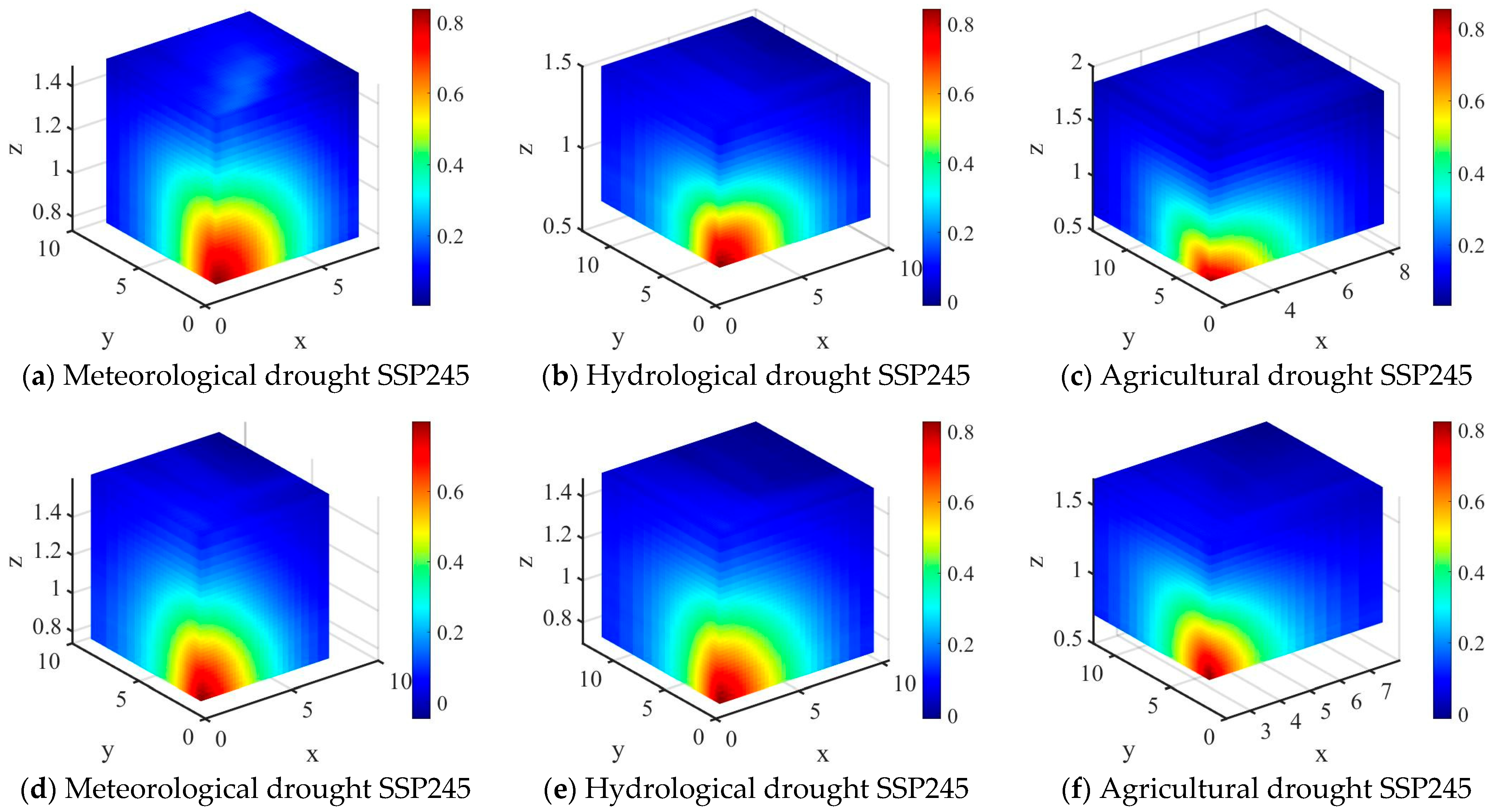
Since the C-Vine copula model is more suitable for scenarios where there are significant dominant dependencies between variables, this paper focuses on multivariate simulation of drought characteristics from the perspective of this model. To quantitatively distinguish the impact of each variable on the risk of drought occurrence, we take the AND scenario as an example:
P ( X x , Y y , Z z ) = 1 F X ( x ) F Y ( y ) F Z ( z ) + C F X ( x ) , F Y ( y ) + C F X ( x ) , F Z ( z ) + C F Y ( y ) , F Z ( z ) C F X ( x ) , F Y ( y ) , F Z ( z ) ] = 1 u v w + C ( u , v ) + C ( u , w ) + C ( v , w ) C ( u , v , w )
In the equation, F X ( x ) , F Y ( y ) , and F Z ( z ) are the cumulative distribution functions of intensity S and cracking P under different drought indices over time D.

3.5.3. Evaluation Indicators and Joint Occurrence Probability

Four evaluation metrics—determination coefficient (R2), root mean square error (RMSE), Akaike information criterion (AIC), and Bayesian information criterion (BIC)—were selected to assess the simulation accuracy of the model. A higher R2 value indicates a stronger correlation between the simulation results and the actual values, while a lower R2 value indicates a weaker correlation. Generally, smaller values of RMSE, AIC, and BIC indicate better model accuracy.
The joint occurrence probability refers to the probability that two events occur simultaneously when multiple random variables in a multivariate probability distribution each satisfy their respective conditions. The calculation of the joint occurrence probability of drought events can be divided into two cases: (1) the “or” case, where the probability that at least one of the variables D, S, and P is greater than or equal to a certain value is denoted as Po; (2) the “and” case, where the probability that all three variables D, S, and P are greater than or equal to a certain value is denoted as Pa.

3.6. Lagged Correlation

Lagged correlation refers to the correlation between two time series at a certain time lag. In this study, for each possible lag value k (k = 1, 2, …, 12 months), the meteorological drought sequence remains unchanged, while the hydrological drought sequence and agricultural drought sequence are shifted backward by k time steps (i.e., hydrological drought and agricultural drought occur k months after meteorological drought) [59]. The Spearman rank correlation coefficient between the shifted sequence combinations is calculated using the following formula:
ρ k = 1 6 t = 1 n k d t 2 n n 2 1
In the formula, d t = R X t R Y t + k is the rank difference between X t and Y t + k at time t, and n is the length of the time series.

3.7. Bayesian Network Probability Model

The Bayesian network probability model effectively addresses uncertainty issues in systems by combining conditional probability methods to estimate the relationships between variables. This paper employs a first-order Bayesian network probability model for the solution. In real-world production and daily life, people are more concerned with the probability of a response from one variable or two variables under certain conditions. For example, consider the conditional probability of mild (moderate or severe) agricultural drought occurring under mild (moderate or severe) meteorological drought conditions. The formula for this probability is:
P ( x 1 < X x 2 | y 1 < Y y 2 ) = C ( F X ( x 1 ) , F y ( y 2 ) ) + C ( F x ( x 1 ) , F y ( y 1 ) ) F y ( y 2 ) F y ( y 1 ) C ( F X ( x 1 ) , F y ( y 2 ) ) + C ( F x ( x 2 ) , F y ( y 1 ) ) F y ( y 2 ) F y ( y 1 )
In the formula, X and Y represent SRI and SAPEI/SSMI, respectively. To further determine the trigger thresholds for different levels of hydrological drought and agricultural drought under meteorological drought conditions, SAPEI is iterated from −0.5 in steps of −0.1, and the corresponding probability p is calculated. When the trigger probability is set to 0.5, i.e., p ≥ 0.5, the iteration is terminated, and the value on the right side of the interval is the transfer threshold.

4. Results Analysis

4.1. SWAT Model Runoff Simulation and CMIP6 Global Climate Model Evaluation

4.1.1. SWAT Model Runoff Simulation Evaluation

The Naoli River basin experienced substantial hydrological variability from 2006 to 2012, characterized by pronounced inter-annual discharge fluctuations. The peak annual discharge recorded in 2010 exceeded the minimum flow observed in 2008 by a factor of five, suggesting considerable temporal instability in the basin’s hydrological regime. This pronounced variability appears to correlate with the progressive decline in wetland coverage within the watershed. A historical analysis reveals a dramatic reduction in wetland extent, declining from 94.4 × 10⁴ hectares in 1954 to 94.4 × 10⁴ hectares by 2005—representing an 81% decrease over five decades. This substantial wetland loss primarily resulted from agricultural conversion, fundamentally altering the basin’s hydrological characteristics. The transformation of natural wetlands to agricultural land use has compromised the basin’s natural flow regulation mechanisms, contributing to enhanced peak discharge events and diminished capacity for flood attenuation [5]. The outcomes of runoff modeling are presented in Supplementary Figure S1.
Model calibration and validation employed monthly streamflow data from the Caizuzi station (2005–2012). SWAT-CUP facilitated the parameter sensitivity analysis, identifying 17 key variables ranked by their influence on simulation performance. Supplementary Table S1 reveals that curve number III, deep aquifer losses, shallow groundwater thresholds, channel geometry, and baseflow coefficients exhibited the highest sensitivity rankings.
The SUFI-2 algorithm generated 95% prediction intervals (L95PPU and U95PPU) for an uncertainty assessment of monthly discharge simulation (2006–2012). Performance metrics demonstrated excellent model accuracy: the calibration period (2006–2008) achieved NSE = 0.98, R2 = 0.82, P-factor = 0.31, PBIAS = −6.18% and the validation period (2009–2012) maintained strong performance with NSE = 0.97, R2 = 0.75, P-factor = 0.42, PBIAS = −9.48%. These results confirm the SWAT model’s suitability for Naoli River basin hydrological modeling applications.

4.1.2. CMIP6 Climate Model Assessment

This investigation employed Taylor diagram analysis to evaluate 15 CMIP6 global climate models against observational records from the Nongli River Basin (1970–2014). Model assessment utilized three statistical metrics: correlation coefficient (r), root mean square error (RMSE), and standard deviation. Performance ranking through Taylor diagram visualization enabled identification of the five highest-performing models for ensemble construction to generate future meteorological forcing data. Taylor diagram comparisons between CMIP6 models and observational data are presented in Supplementary Figure S2.
The top-performing models—EC-Earth3, IPSL-CM6A-LR, MPI-ESM1-2-HR, MPI-ESM1-2-LR, and NorESM2-MM—were combined through ensemble averaging to develop an optimized multi-model ensemble (MMM-Best). This composite model demonstrated superior statistical performance, with the strongest positive correlation (r = 0.80), minimal root mean square error (RMSE = 26.15), and standard deviation closely matching observational data (41.28). Consequently, MMM-Best was adopted as the primary climate model for projecting annual precipitation and temperature variations across the Rao River basin under various emission scenarios throughout 2025–2100.

4.2. Single-Variable Drought Characteristics of the Rao River Basin

Table 4 presents drought characteristics under the SSP245 scenario across two temporal periods. During the early projection period (2025–2050), drought occurrence remained relatively infrequent, with SPAEI recording 22 episodes, SRI documenting 17 events, and SSMI capturing 20 occurrences. The mean duration ranged from 3.91 to 5.40 days. The average severity spanned 4.27 to 6.90, and the mean intensity varied between 1.01 and 1.18. The subsequent period (2051–2100) demonstrated a substantial increase in drought frequency, with SPAEI events rising to 41, SRI episodes reaching 36, and SSMI occurrences totaling 29. Duration patterns exhibited mixed trends: the SPAEI showed modest extension to 4.15 days, whereas the SRI and SSMI displayed reductions to 4.72 and 4.34 days, respectively. Severity metrics revealed contrasting trajectories, with SPAEI intensifying to 4.93, while SRI and SSMI diminished to 5.20 and 5.60, respectively. Intensity measurements indicated marginal increases for SPAEI (1.12) and SSMI (1.15), contrasted by a decrease in SRI (0.99). Under this moderate emission pathway, drought frequency escalated markedly in the latter half-century, while the duration and severity parameters showed amelioration, accompanied by minimal intensity fluctuations.
Under the SSP585 scenario, the initial projection period (2025–2050) demonstrated consistent drought frequency across all indices (21 events each), with mean durations spanning 4.14–4.48 days, average severity ranging from 5.12–5.37, and mean intensity varying between 1.06–1.12. The subsequent period (2051–2100) revealed increased drought occurrence, with SPAEI documenting 38 episodes, SRI recording 33 events, and SSMI capturing 35 occurrences. The duration patterns exhibited contrasting behaviors: SPAEI showed a reduction to 4.03 days, SRI demonstrated a substantial extension to 5.73 days, and SSMI displayed modest increases to 4.46 days. The severity metrics revealed divergent trends, with SPAEI declining to 4.67, contrasted by escalations in SRI (6.16) and SSMI (5.78). Intensity measurements indicated increases for SPAEI (1.18) and SSMI (1.19), while SRI exhibited a reduction to 1.02. Under this high-emission pathway, drought characteristics in the latter period demonstrated overall intensification across frequency, duration, severity, and intensity parameters.
The SSP245 scenario exhibited substantially increased drought frequency, yet duration, severity, and intensity parameters generally diminished, with particularly notable improvements observed in the SRI and SSMI metrics. Conversely, the SSP585 scenario demonstrated escalating trends across drought frequency, SRI duration, severity, and intensity, indicating heightened drought hazards during the latter phase of high-emission trajectories. This intensification particularly affects hydrological and pedological moisture conditions, emphasizing the necessity for enhanced targeted drought management strategies.

4.3. Plus Land Use Simulation and Evaluation

A land use transformation analysis through Sankey diagrams spanning 2000–2020 (detailed in Supplementary Material Figure S3) reveals substantial alterations in the Zhili River basin’s spatial configuration, with notable reductions in arable land, grassland, and construction areas by 327.26 km2, 13.81 km2, and 151.63 km2, respectively, while unutilized terrain experienced minimal expansion of merely 0.26 km2. Conversely, aquatic systems and forested regions demonstrated pronounced growth trajectories, expanding by 388.65 km2 and 103.80 km2, respectively, underscoring the substantial effectiveness of wetland conservation initiatives within the basin and their pivotal influence on future land use evolution. Employing the LEAS module within the PLUS modeling framework, spatial distribution forecasting of 14 land use transformation drivers was conducted using 2010 as the reference baseline, yielding robust validation metrics, including a Kappa coefficient of 0.85, an overall accuracy of 0.93, and a FoM coefficient of 0.08, confirming the model’s reliability for projecting land use dynamics in the Zhili River basin. Maintaining consistent model parameters and driver relationships, the PLUS framework generated land use pattern projections for 2040–2080 (illustrated in Supplementary Figure S4), indicating that forthcoming transformations will perpetuate the 2000-2020 trajectory, predominantly featuring continued expansion of aquatic and forested areas alongside a gradual contraction of grasslands, construction zones, and alternative land categories, reflecting the persistence of governmental policies, particularly intensive water body and forest conservation measures. As shown in the figure demonstrates that, under SSP245 conditions, agricultural land experiences a sustained but moderate decline across temporal intervals, maintaining approximately 7.8% reduction rates. Forested areas exhibit consistent expansion compared to baseline conditions, with roughly 9.1% growth patterns. Notably, water body expansion proves most pronounced, achieving approximately 12.7% increases across all projected periods. The SSP585 scenario presents similar agricultural land trends, with reductions of 2.3%, 3.7%, and 4.8% across different temporal phases. Forest coverage continues expanding at rates of 5.7%, 9.1%, and 11.9% for 2040, 2060, and 2080, respectively. Grassland areas decline while stabilizing around 5.5%; aquatic regions remain relatively stable, whereas urban development maintains growth momentum at 0.11%, 0.18%, and 0.2% for the respective projection years, resulting from the combined influences of SSP585 scenario conditions and regional policy frameworks.

4.4. Marginal Distributions of Different Drought Characteristic Variables

The AIC test results for the fitted distributions of drought duration, drought intensity, and peak drought intensity for different types of droughts in the Rao River Basin during the periods 2025–2050 and 2051–2100 are shown in Table 5. The distribution corresponding to the smallest AIC value was selected as the optimal fitted distribution for the given drought characteristic variable, i.e., the marginal distribution.

4.5. Copula Functions for Multidimensional Drought Characteristic Variables

Based on AIC, BIC, RMSE, and K-S criteria, the optimal copula functions for various combinations of drought-characteristic variables in the Naoli River Basin for the periods 2025–2050 (near term) and 2051–2100 (long term) were determined (See Supplementary Materials Tables S2–S7 for details). The optimal copula function selection under SSP245 scenarios is, for meteorological drought, the D–S variable combination maintains the Gaussian function in both the near term and long term. The D–P combination transitions from the Clayton function in the near term to the Frank function in the long term, while the S–P combination transitions from the Clayton function in the near term to the Gaussian function in the long term. In terms of hydrological drought, both the D–S and D–P combinations undergo a change in function type: D–S changes from Clayton in the near term to Gaussian in the far term, and D–P changes from Clayton in the near term to Frank in the far term. The S–P combination changes from the Gumbel function in the near term to the Frank function in the far term. In terms of agricultural drought, all feature variable combinations use the Clayton function in the short term. In the long term, only the S–P combination changes to the Gaussian function, while the D–S and D–P combinations remain unchanged at the Clayton function. For the optimal copula function selection under the SSP585 scenario, in terms of meteorological drought, the D–S feature variable combination changes from the Gaussian function in the short term to the Gumbel function in the long term. The D–P and S–P combinations both uniformly transition from the Frank and Clayton functions in the near term to the Clayton function in the long term. For hydrological drought, the D–S feature variable combination remains unchanged at the Gaussian function in both the near term and long term. The D–P combination transitions from the Gaussian function in the near term to the Gumbel function in the long term, while the S–P combination transitions from the Clayton function in the near term to the Gaussian function in the long term. For agricultural drought, all feature variable combinations use the Gaussian function in the near term. In the long term, only the D–P combination transitions to the Clayton function, while the D–S and S–P combinations remain unchanged with the Gaussian function.
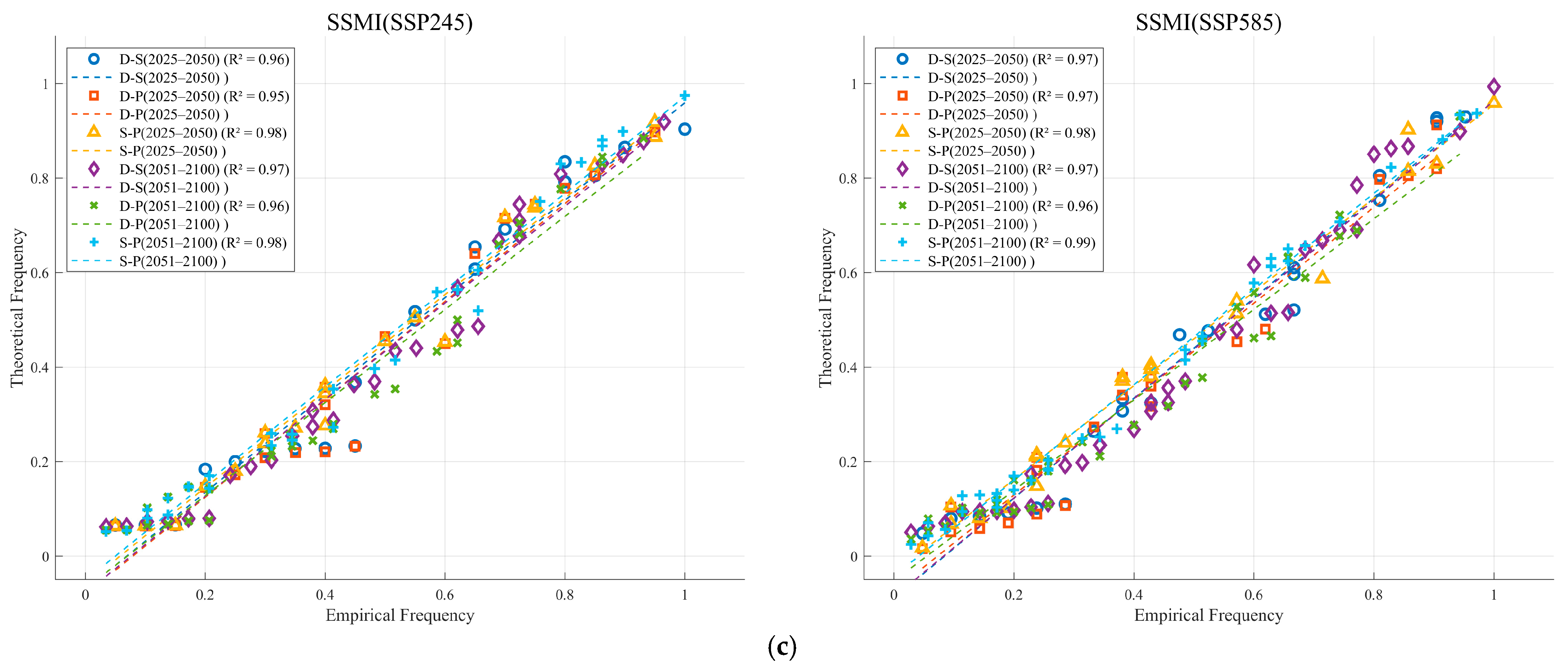
Figure 2 shows the empirical frequency and theoretical frequency relationships of the multidimensional drought variables under the three types of droughts based on the optimal Copula function. As can be seen from the figure, the theoretical frequency and empirical frequency show good consistency under the two scenarios for the three types of droughts, indicating that the results of the optimal Copula function are reasonable and reliable.

4.6. Probability of Joint Occurrence of Drought Under Different Combinations of Characteristic Variables

4.6.1. Two-Dimensional Probability of Joint Occurrence of Drought

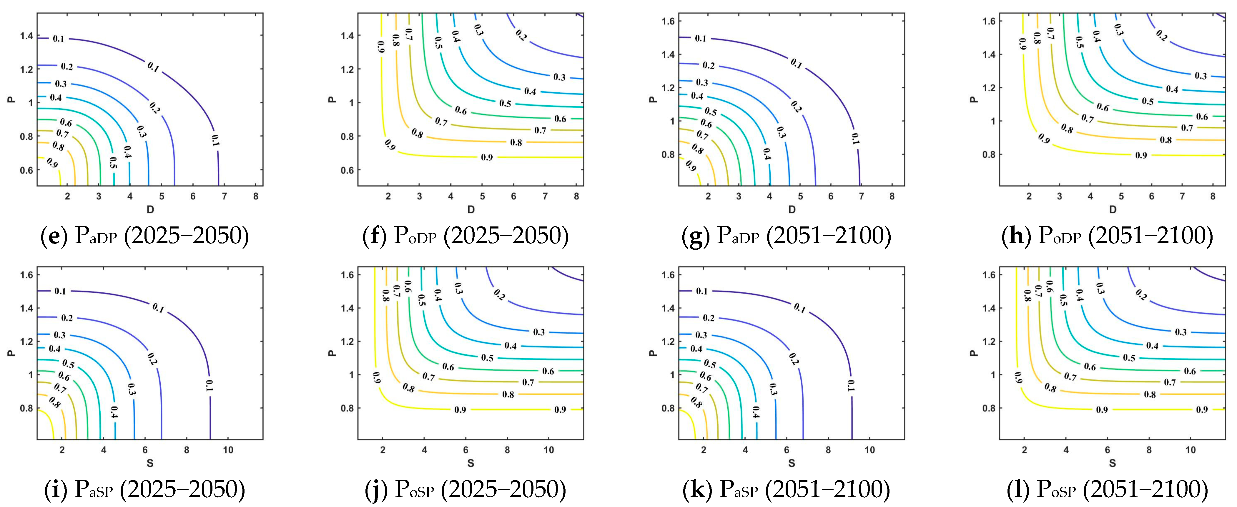
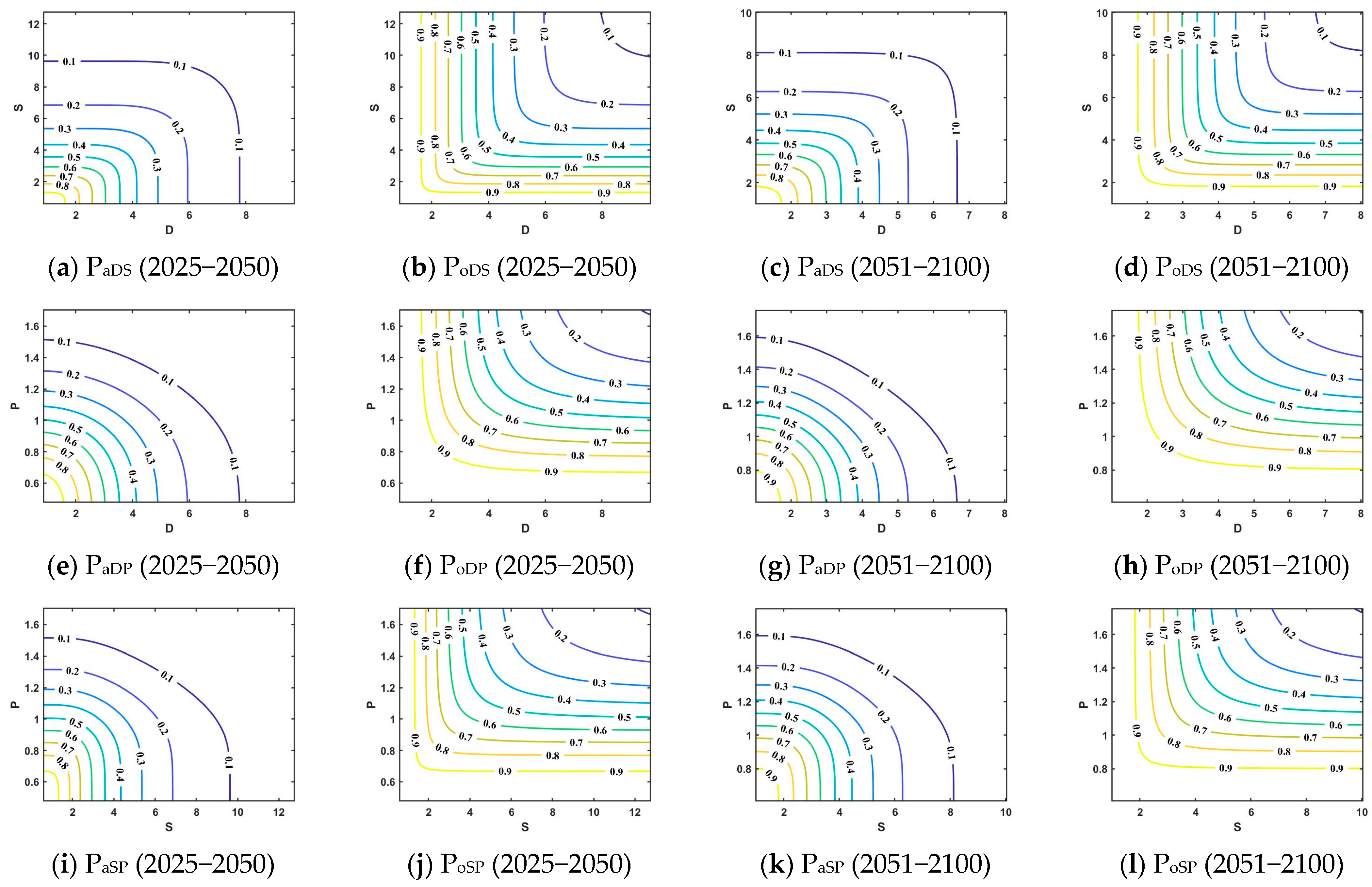
Figure 3 and Figure 4, along with Supplementary Figures S5 and S6, present the two-dimensional drought co-occurrence probabilities of drought characteristic variable combinations (D–S, D–P, and S–P) in the lower reaches of the Songhua River basin under different scenarios and time periods. Overall, the probability of joint drought occurrence decreases gradually as the values of drought characteristic variables increase. When one variable is fixed, an increase in the other variable leads to a synchronous decrease in the joint drought probability under both “or” and “and” conditions.
To further assess the evolution trend of drought co-occurrence, this study ranked the single-variable drought characteristic values within the basin during the 2025–2100 period by frequency and calculated the cumulative frequency. Thresholds corresponding to cumulative frequencies of 75%, 50%, and 25% were selected to represent mild, moderate, and severe drought levels (see Table 6). Based on this, the multidimensional drought occurrence probabilities corresponding to different levels of single-variable characteristics were calculated for the two time periods (2020–2060 and 2061–2100), and a comparative analysis was conducted.
Under the SSP245 scenario, the meteorological drought D–S combination occurs under mild drought conditions (cumulative frequency of 75%, i.e., D and S are greater than February and 2.07, respectively), and the probability of concurrent occurrence of drought under the “and” and “or” conditions is 0.80 and 0.87, respectively, in the 2061–2100 period, an increase of 0.06 and 0.01 compared to the 2020–2060 period. Under moderate drought conditions (cumulative frequency of 50%, with D and S exceeding March and 3.27, respectively), the probabilities under the “and” and “or” conditions are 0.56 and 0.66, respectively, with increases of 0.05 and 0.03. Under severe drought conditions (cumulative frequency of 25%, D and S greater than 5 months and 5.86, respectively), the probabilities of “and” and “or” are 0.21 and 0.30, respectively, with increases of 0.02 and 0.03 compared to the previous period. This indicates that the D–S combination has a higher probability of concurrent occurrence in the long term compared to the short term, with the most significant increase under moderate drought conditions. The D–P combination under both “and” and “or” conditions showed increases in the 2061–2100 period compared to the 2020–2060 period, with growth rates of 0.11 and 0.06, 0.10 and 0.08, and 0.05 and 0.08, respectively, at cumulative frequencies of 75%, 50%, and 25%. The most significant change occurred at the 75% frequency. The joint probability of the S–P combination also showed an increasing trend under all three drought severity levels. Under the “and” and “or” conditions, the growth rates corresponding to cumulative frequencies of 75%, 50%, and 25% were 0.12 and 0.11, 0.13 and 0.13, and 0.09 and 0.09, respectively, with the largest change occurring at the 50% frequency. Under the SSP585 scenario, the combined drought probability of the D–S combination showed a slight increasing trend at 75% and 50% frequencies under the “and” and “or” conditions, increasing by 0.06 and 0.05, and 0.01 and 0.02, respectively. However, at 25% frequency, it showed a decreasing trend, with reduction magnitudes of -0.02 and -0.03; The D–P combination showed changes in the joint drought probability under the “and” and “or” conditions at 75%, 50%, and 25% frequency, with changes of 0.14 and 0.04, 0.06 and 0.07, and 0.001 and 0.04, respectively, indicating the most significant changes under mild drought conditions. The joint occurrence probability of the S–P combination increased under different drought severity levels, with the most significant increase at a cumulative frequency of 75%, with growth rates of 0.15 and 0.10. Under 50% and 25% frequencies, the changes were relatively mild, at 0.09 and 0.11, and 0.02 and 0.05, respectively.
In terms of hydrological drought, under the SSP2-5.8 scenario, the long-term joint drought probability generally decreased compared to the short-term, with the only exception being the D–P combination at a 75% frequency under the “or” condition, which showed a slight increase (+0.007), while all others decreased. In the D–S combination, the most significant decreases occur at a cumulative frequency of 50% under the “and” and “or” conditions, with changes of −0.12 and −0.14, respectively. The most significant decrease in the D–P combination also occurs at a frequency of 50%, with changes of −0.15 and −0.11, respectively. In the S–P combination, the most severe decline occurred at a frequency of 25%, with a change value of −0.16 (both “and” and “or” were the same). In the SSP585 scenario, the overall joint drought probability showed an increasing trend, with only the S–P combination showing a decline at a frequency of 25% (“and” and “or” were −0.03 and −0.14, respectively). Among these, the D–S combination showed the largest increase at a 50% frequency, with values of 0.23 and 0.18. The D–P combination exhibited the most significant increase at a 75% frequency, with values of 0.16 and 0.13.
In terms of agricultural drought, the changes in different feature combinations under the SSP245 scenario vary: the D–S combination exhibits the largest change in the probability of combined drought at a 25% frequency, with values of −0.12 and −0.09; the D–P combination shows the most significant change at a 50% frequency, with values of −0.12 and +0.03; and the S–P combination also exhibits its largest changes at a 50% frequency, with values of −0.05 and +0.02, respectively.

4.6.2. Probability of Simultaneous Occurrence of Three-Dimensional Drought

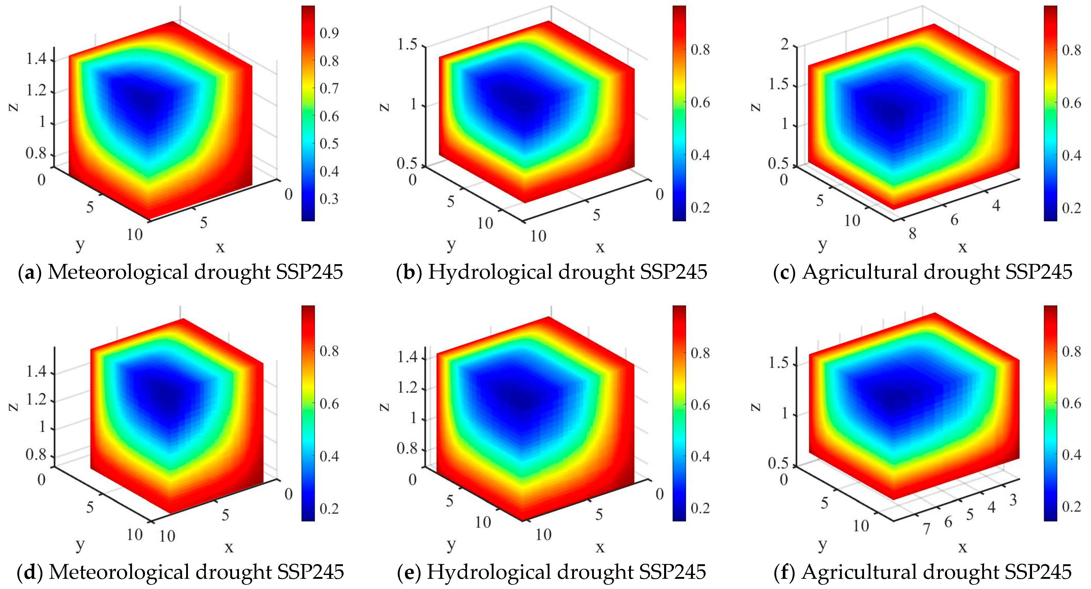
Figure 5 and Figure 6 show the three-dimensional probability of joint occurrence of meteorological drought under the conditions of “or” and “and” in different scenarios. The figures show that, as the cumulative frequency of drought characteristics increases, the probability of joint occurrence of drought gradually decreases.
Under the meteorological drought SSP245 scenario, we conducted a frequency analysis of single-variable drought characteristics from 2025 to 2100 and calculated the multidimensional drought joint occurrence probability corresponding to single-variable drought characteristics in different time periods. When the cumulative frequency of single variables reaches 75%, i.e., when D, S, and P exceed 2 months, 2.07, and 0.88, respectively, the three-dimensional drought co-occurrence probability P o D S P under the “or” condition and the three-dimensional drought co-occurrence probability P a D S P under the “and” condition are 0.953 and 0.69, respectively. When the cumulative frequency of a single variable reaches 50%, i.e., when D, S, and P exceed 3 months, 3.27, and 1.03, respectively, P o D S P and P a D S P are 0.80 and 0.48, respectively. When the cumulative frequency of a single variable reaches 25%, i.e., when D, S, and P exceed 5 months, 5.86, and 1.20, respectively, P o D S P and P a D S P are 0.52 and 0.23, respectively. Under the SSP585 scenario, when the single-variable cumulative frequencies are 75%, 50%, and 25%, i.e., when D, S, and P exceed 2 months, 2.30, and 0.89, respectively; 3 months, 3.63, and 1.09; and 4 months, 5.60, and 1.31, respectively, the three-dimensional drought joint occurrence probability under the “or” condition and the “and” condition are P o D S P and P a D S P , respectively: 0.90 and 0.56, 0.72 and 0.28, and 0.55 and 0.11. It can be seen that, under the SSP245 scenario, the joint occurrence probability is higher when the single-variable cumulative frequency is 75% and 50%, whereas under the SSP585 scenario, the joint occurrence probability is higher when the single-variable cumulative frequency is 25%.
Under the hydrological drought SSP245 scenario, when the single-variable cumulative frequency reaches 75%, i.e., when D, S, and P exceed 2 months, 1.90, and 0.80, respectively, P o D S P and P a D S P are 0.89 and 0.66, respectively. When the cumulative frequency of a single variable reaches 50%, i.e., when D, S, and P exceed 4 months, 3.87, and 0.97, respectively, P o D S P and P a D S P are 0.67 and 0.34, respectively. When the cumulative frequency of a single variable reaches 25%, i.e., when D, S, and P exceed 6 months, 6.22, and 1.17, respectively, P o D S P and P a D S P are 0.42 and 0.12, respectively. Under the SSP585 scenario, when the single-variable cumulative frequency reaches 75%, i.e., when D, S, and P exceed 2 months, 2.32, and 0.84, respectively, P o D S P and P a D S P are 0.92 and 0.62, respectively. When the single-variable cumulative frequency reaches 50%, i.e., when D, S, and P exceed 3.5 months, 3.33, and 1.00, respectively, P o D S P and P a D S P are 0.76 and 0.39, respectively. When the single-variable cumulative frequency reaches 25%, i.e., when D, S, and P exceed 6 months, 6.08, and 1.21, respectively, P o D S P and P a D S P are 0.43 and 0.10, respectively. It can be seen that, under the SSP585 scenario, the joint occurrence probability is highest when the single-variable cumulative frequency is 75% and 50%. However, when the single-variable cumulative frequency is 25%, the P o D S P probability is higher under the SSP245 scenario, while the P a D S P probability is higher under the SSP585 scenario.
Under the agricultural drought SSP258 scenario, when the single-variable cumulative frequency reaches 75%, 50%, and 25%, i.e., when D, S, and P exceed 3 months, 2.15, and 0.74; April, 4.13, and 0.92; and July, 9.26, and 1.42, respectively, the three-dimensional drought co-occurrence probability under the “or” condition ( P o D S P ) and under the “and” condition ( P a D S P ) are 0.85 and 0.65, 0.67 and 0.43, and 0.30 and 0.12, respectively. Under the SSP585 scenario, when the cumulative frequency of a single variable reaches 75%, i.e., when D, S, and P exceed 2, 2.29, and 0.85, respectively, P o D S P and P a D S P are 0.96 and 0.64, respectively. When the single-variable cumulative frequency reaches 50%, i.e., when D, S, and P exceed 4 months, 4.01, and 1.02, respectively, P o D S P and P a D S P are 0.66 and 0.28, respectively. When the single-variable cumulative frequency reaches 25%, i.e., when D, S, and P exceed 5.5 months, 6.64, and 1.34, respectively, P o D S P and P a D S P are 0.39 and 0.10, respectively. It can be seen that, under the SSP585 scenario, the joint probability of P o D S P is highest when the single-variable cumulative frequency reaches 75% and 25%. In other cases, the probabilities of P o D S P and P a D S P are higher under the SSP245 scenario.

4.6.3. Time and Threshold for the Transition of Meteorological Drought to Hydrological and Agricultural Drought

This study selected the SPAEI, SRI, and SSMI indices at time scales of 3, 6, and 12 months, calculated their lagged correlations, and explored the transmission process of meteorological drought to hydrological drought and agricultural drought. Under the SSP245 scenario, the transmission times from meteorological drought to hydrological drought and agricultural drought are as follows: 7 months and 3 months at the 3-month timescale, 3 months and 3 months at the 6-month timescale, and 5 months and 4 months at the 12-month timescale; Under the SSP585 scenario, the transmission times are as follows: 6 months and 2 months at the 3-month scale, 5 months and 3 months at the 6-month scale and 2 months and 4 months at the 12-month scale.
In terms of drought severity classification, under the SSP245 scenario, the threshold for mild hydrological drought is −1.5, with thresholds for moderate, severe, and extreme drought at −2.6, −3.3, and −3.8, respectively. The thresholds for mild, moderate, severe, and extreme agricultural drought are −1.1, −1.7, −2.2, and −2.6, respectively. Under the SSP585 scenario, the thresholds for mild, moderate, severe, and extreme agricultural drought are −1.1, −2.5, −3.9, and −4.6, respectively. Under the SSP245 scenario (agricultural drought), the corresponding thresholds are −1.0, −1.9, −2.5, and −3.0.

4.6.4. Transmission Risks from Meteorological Drought to Hydrological Drought and Agricultural Drought

Table 7 and Table 8 present the conditional probabilities of hydrological drought and agricultural drought (both with severity levels ranging from 2 to 5) triggered by meteorological drought (severity levels 2 to 5 representing mild, moderate, severe, and extreme drought, respectively) under the SSP245 and SSP585 climate change scenarios, respectively. As shown in Table 7, under the SSP245 scenario, the conditional probability of hydrological drought across all severity levels generally increases with the severity of meteorological drought. Specifically, as meteorological drought severity increases from mild (2) to extreme (5), the conditional probability of mild hydrological drought (level 2) remains relatively stable (range 0.17–0.19), while the conditional probability of moderate and severe hydrological drought (levels 3–5) significantly increases. Among these, extreme hydrological drought (level 5) exhibits the most pronounced trend, with its conditional probability rising significantly from 0.03 at meteorological drought level 2 to 0.17 at level 5, indicating that extreme meteorological drought events significantly increase the probability of extreme hydrological drought occurrence. Under the SSP585 scenario, the conditional probabilities of hydrological drought at all levels increase more markedly and steadily with the severity of meteorological drought. The conditional probability of mild hydrological drought gradually increased from 0.19 to 0.21, while the probability of moderate (level 3) and severe (level 4) hydrological drought showed a clear upward trend, rising from 0.12 and 0.06 to 0.19 and 0.14, respectively. The conditional probability of extreme hydrological drought reaches its highest value of 0.12 under extreme meteorological drought scenarios, significantly higher than that under mild meteorological drought scenarios (0.03), indicating the significant driving role of extreme meteorological drought in severe hydrological drought under high emission conditions.
For agricultural drought, Table 8 reveals similar, but more complex, trends. Under the SSP245 scenario, the conditional probabilities of agricultural drought across all severity levels generally increase with a higher meteorological drought severity, with this trend becoming more pronounced at more severe agricultural drought severity levels (levels 4 and 5). Taking extreme agricultural drought (grade 5) as an example, its conditional probability significantly increases from 0.03 at meteorological drought grade 2 to 0.12 at meteorological drought grade 5, indicating the significant driving role of extreme meteorological drought in agricultural drought. Under the SSP585 scenario, the trend in the conditional probability of agricultural drought shows certain differences. The probability of moderate to severe agricultural drought (levels 3–4) increases steadily as meteorological drought intensity increases, particularly for severe agricultural drought (level 4), whose conditional probability rises significantly from 0.04 under mild meteorological drought to 0.15 under extreme meteorological drought, while the conditional probability of extreme agricultural drought (grade 5) reaches its highest value (0.24) under extreme meteorological drought scenarios, significantly higher than the probability corresponding to the SSP245 scenario (0.12). This indicates that, under future high-emission scenarios, extreme meteorological drought significantly increases the risk of extreme drought events in the agricultural sector. However, it is important to note that, under the SSP585 scenario, the probability of extreme agricultural drought corresponding to mild meteorological drought conditions (0.02) is slightly lower than that under the SSP245 scenario (0.03), suggesting that the differences in agricultural drought risks between the two emission scenarios are relatively small under less-severe drought conditions, but significantly widen under extreme conditions.
Based on the above analysis, it can be concluded that, under different future climate change scenarios, the severity of meteorological drought is positively correlated with the probability of hydrological drought and agricultural drought. In particular, under extreme meteorological drought conditions, the conditional probability of extreme hydrological drought and extreme agricultural drought significantly increases, and this increasing trend is more pronounced under high emission scenarios (SSP585). This suggests that future drought management and climate adaptation policies should pay particular attention to the potential risks of extreme drought to enhance the effectiveness of regional drought risk response and management.

5. Discussion

This study uses the Naoli River basin as a case example to systematically analyze the spatiotemporal evolution characteristics of meteorological, agricultural, and hydrological droughts under different future emission scenarios (SSP245 and SSP585). The results indicate that, regardless of the scenario, the frequency of drought events will significantly increase in the future, particularly under high-emission scenarios, where the duration, intensity, and severity of droughts all exhibit a worsening trend. This finding is consistent with simulation results from other drought-sensitive regions worldwide, such as the North American Great Plains and the Murray–Darling Basin in Australia, which have also reported simultaneous increases in the frequency and intensity of extreme drought events in the future [60,61]. Mechanistically, this trend is not only influenced by reduced total precipitation and increased frequency of extreme climate events, but also closely related to large-scale wetland loss and significant changes in land use patterns in the region. Since the mid-20th century, large-scale wetland loss in this region has led to a decline in hydrological regulation functions, significantly weakening the basin’s buffering capacity against climate anomalies [62,63].
Compared with traditional univariate or linear correlation models, the advantages of copula functions in modeling multidimensional drought correlations are further highlighted. The results of this study indicate that copula models can effectively reveal the nonlinear dependency structure among meteorological, agricultural, and hydrological droughts and quantify the joint occurrence probability under different combinations of characteristic variables. The theoretical frequency is highly consistent with the empirical frequency, indicating that the model has high reliability. Internationally, the application of copula methods in drought risk management has gradually increased in recent years, particularly demonstrating superiority in joint risk assessment in multi-river basins in Europe and agricultural regions in the Western United States [59,64]. This study confirms that the method has practical significance for joint extreme event risk warning in complex watershed scenarios. The PLUS model predictions indicate that, in the future, forest and water body areas in the Naoli River basin will increase, while arable land and construction land will further decrease. This pattern change reflects the effectiveness of government wetland protection and ecological restoration policies, which help improve regional hydrological stability. However, the mitigation effect of land use optimization on drought risk is limited under high emission scenarios, suggesting that the impact of climate change may gradually exceed the regulatory capacity of land management measures. This conclusion resonates with domestic and international empirical studies on wetland restoration and land use management, emphasizing the need for a coordinated advancement of ecological restoration and climate adaptation policies. A lag correlation analysis of multi-dimensional drought indices revealed significant time lags in the transmission of meteorological drought to hydrological and agricultural drought, with varying transmission durations across different scenarios and time scales. For example, under high-emission scenarios, the transmission time of hydrological drought can be shortened to 2–6 months, suggesting that extreme meteorological events accelerate the response of river runoff and soil moisture. This conclusion provides important reference for regional agricultural irrigation scheduling and water resource management early-warning systems. It is recommended that management departments enhance meteorological drought monitoring and early-warning systems and integrate multi-source information across river basins to achieve dynamic control of drought risks at multiple scales.
However, this study also has limitations. For example, the SWAT model is constrained by the length of hydrological observation data in the watershed, which may affect the accuracy of long-term simulation. Furthermore, the joint distribution assumption of the copula model still differs from the complexity of actual drought processes. In the future, multi-source methods such as remote-sensing inversion, field measurements, and machine learning can be combined to further improve the scientific and practical nature of regional drought risk quantification and response regulation.
This study indicates that strengthening wetland protection in river basins, promoting the optimization of land use structures, and enhancing multi-dimensional drought management are effective strategies for mitigating the risks of future extreme droughts in the context of climate change. Specifically for agricultural drought management, the study recommends establishing crop-specific drought-monitoring networks, developing precision irrigation systems based on real-time soil moisture data, and implementing drought-resilient agricultural practices, including cover cropping and soil organic matter enhancement. These measures could reduce agricultural drought vulnerability by 20–30% while maintaining ecosystem service benefits from wetland restoration. It is recommended that relevant departments incorporate the copula multivariate joint risk assessment method into the regional water resources and food security comprehensive decision-making system to enhance risk forecasting and resilience management capabilities. At the same time, efforts should be made to continuously improve the acquisition of multi-source data and model accuracy in river basins and promote the deep integration of high-resolution climate scenarios and land use scenario simulations.

6. Conclusions

(1) The SWAT modeling framework exhibits robust applicability in streamflow simulation for the Zhaoli River basin, providing a reliable technical foundation for hydrological forecasting, with the coefficient of determination R2 exceeding 0.75 and the Nash–Sutcliffe efficiency coefficients surpassing 0.97 during both the calibration and validation phases. Simultaneously, the PLUS modeling approach demonstrates exceptional adaptability in basin-scale land use simulation, achieving overall accuracy above 0.93 and Kappa coefficients greater than 0.85;
(2) Future land use evolution analysis reveals that forested areas will experience sustained expansion across different scenario conditions, while agricultural lands exhibit declining trends under all examined scenarios. The SSP245 pathway indicates significant expansion of aquatic areas, whereas the SSP585 scenario projects gradual increases in urban development zones;
(3) Fifteen CMIP6 modeling systems provided dependable temperature forecasting capabilities for the Raohe River basin spanning 1970–2014 (correlation coefficient r > 0.97, root mean square error RMSE < 2.98), with EC-Earth3, IPSL-CM6A-LR, MPI-ESM1-2-HR, and MPI-ESM1-2-LR demonstrating superior performance. The NorESM2-MM framework showed exceptional precipitation forecasting accuracy (r > 0.75, RMSE < 30.99, standard deviation ≈ 41.28), with its ensemble-averaged MMM-Best configuration (r = 0.80, RMSE = 26.15) identified as the optimal forecasting system for the 2025–2100 projection period;
(4) Under different scenarios (SSP245 and SSP585) in the Naoli River basin, the optimal copula functions selected based on AIC, BIC, RMSE, and K-S criteria effectively fitted the joint distributions of various drought types (meteorological, hydrological, and agricultural) and their multidimensional characteristic variables. The theoretical frequencies were highly consistent with empirical frequencies, validating the rationality and reliability of the copula function selection;
(5) Based on the analysis of drought characteristic variable combinations (D–S, D–P, and S–P) under different scenarios (SSP245 and SSP585) in the lower reaches of the Songhua River basin, the joint occurrence probability of drought generally shows a trend of change over time. In terms of meteorological drought, compared with the recent period (2020–2060), the joint drought probability in the long term (2061–2100) mostly showed an upward trend, with the most significant increase under moderate drought conditions. In terms of hydrological and agricultural droughts, the probability of concurrent droughts decreased in the long term (2061–2100) under the SSP245 scenario, while it generally increased under the SSP585 scenario, particularly under mild drought conditions. Overall, the trends in the probability of concurrent droughts are closely related to different scenarios, different frequencies, and different drought severity levels, with significant differences in the responses of various drought types;
(6) Under different scenarios (SSP245 and SSP585), the three-dimensional joint occurrence probability of meteorological, hydrological, and agricultural droughts gradually decreases with the increase in the cumulative frequency of drought characteristic variables. Specifically, in the SSP245 scenario, the joint occurrence probability of meteorological drought is higher at cumulative frequencies of 75% and 50%, while in the SSP585 scenario, the joint occurrence probability is higher at a frequency of 25%. For hydrological drought, the joint occurrence probability is most significant at 75% and 50% frequency under the SSP585 scenario. In agricultural drought, the joint occurrence probability is higher at 75% frequency under the SSP585 scenario, while at 25% frequency, it tends to be higher under the SSP245 scenario. Overall, the joint drought probability under various scenarios exhibits different trends under different cumulative frequency conditions of drought severity and demonstrates distinct response patterns across different types of droughts;
(7) As the severity of meteorological drought increases, the conditional probabilities of hydrological drought and agricultural drought show a clear positive correlation, particularly under extreme meteorological drought conditions, where the conditional probability of extreme hydrological drought reaches 0.17 and 0.12 under the SSP245 and SSP585 scenarios, respectively, while the conditional probability of extreme agricultural drought is 0.12 and 0.24, respectively, significantly higher than the probabilities under mild meteorological drought conditions (0.03 and 0.02). Notably, the risk amplification effect of extreme agricultural drought is more pronounced under the high-emission SSP585 scenario, with its occurrence probability under extreme meteorological drought conditions being 100% higher than that under the SSP245 scenario. This indicates that the risk of extreme drought facing agricultural systems under future climate change will significantly increase, necessitating prioritized attention to drought risk management and climate adaptation strategies.

Supplementary Materials

The following supporting information can be downloaded at: https://www.mdpi.com/article/10.3390/su17188219/s1, Figure S1. Runoff simulation and evaluation. Figure S2. Taylor plots of rainfall, maximum temperature, and minimum temperature in the Niao River basin from 1970 to 2014 simulated by CMIP6 relative to the observation site. Figure S3. Land use Sankey diagram from 2000 to 2020. Note: Fig. shows only the changes in land use types. Figure S4. SSP typical scenario land use prediction distribution. Figure S5. Probability map of short-term and long-term SRI drought characteristic variables under the SSP245 scenario. Figure S6. Probability map of short-term and long-term SRI drought characteristics variables in the SSP585 scenario. Table S1. Parameter values of SWAT model in Nao li River Basin. Table S2. Multidimensional drought severity classification criteria. Table S3. Copula function parameters for combinations of drought characteristic variables in the near and long term under the SSP245 scenario under meteorological drought conditions. Table S4. Copula function parameters for combinations of drought characteristic variables under the SSP245 scenario in the short and long term under hydrological drought conditions. Table S5. Copula function parameters for combinations of drought characteristic variables under the SSP245 scenario in the short and long term under agricultural drought conditions. Table S6. Copula function parameters for combinations of drought characteristic variables in the near and long term under the SSP585 scenario under meteorological drought conditions. Table S7. Copula function parameters for combinations of drought characteristic variables under the SSP585 scenario in the short and long term under hydrological drought conditions. Table S8. Copula function parameters for combinations of drought characteristic variables under the SSP585 scenario in the short and long term under agricultural drought conditions.

Author Contributions

T.L.: Conceptualization, methodology, software, data gathering, formal analysis, investigation, validation, writing original draft preparation, review, and editing. Z.S.: Supervision, conceptualization, validation, review, and editing. Y.Z.: Validation and review. J.W.: Validation, review, and editing. Y.L.: Review and editing. L.W.: Data curation. All authors have read and agreed to the published version of the manuscript

Funding

This project was funded by the National Natural Science Foundation of China (Grant No. 52079050).

Institutional Review Board Statement

Not applicable.

Informed Consent Statement

Not applicable.

Data Availability Statement

The raw data supporting the conclusions of this article will be made available by the authors on request.

Conflicts of Interest

Authors Yan Liu and Longfei Wang were employed by the company Heilongjiang Provincial Water Resources Research Institute. The remaining authors declare that the research was conducted in the absence of any commercial or financial relationships that could be constructed as a potential conflict of interest.

References

  1. Yu, H.; Wang, L.; Zhang, J.; Chen, Y. A Global Drought-Aridity Index: The Spatiotemporal Standardized Precipitation Evapotranspiration Index. Ecol. Indic. 2023, 153, 110484. [Google Scholar] [CrossRef]
  2. Guo, Y.; Huang, S.; Huang, Q.; Leng, G.; Fang, W.; Wang, L.; Wang, H. Propagation Thresholds of Meteorological Drought for Triggering Hydrological Drought at Various Levels. Sci. Total Environ. 2020, 712, 136502. [Google Scholar] [CrossRef]
  3. DeGuzman, K.; Knappenberger, T.; Brantley, E.; Olshansky, Y. Estimating Runoff Probability from Precipitation Data: A Binomial Regression Analysis. Hydrol. Process. 2023, 37, e15029. [Google Scholar] [CrossRef]
  4. Wu, Q.; Xie, T.; Liu, C.; Li, W.; Zhang, L.; Ran, G.; Xu, Y.; Tang, Y.; Han, Z.; Hu, C. Improving the Understanding of Rainfall-Runoff Processes: Temporal Dynamic of Event Runoff Response in Loess Plateau, China. J. Environ. Manag. 2025, 375, 123436. [Google Scholar] [CrossRef]
  5. Yao, Y.; Wang, L.; Lv, X.; Yu, H.; Li, G. Changes in Stream Peak Flow and Regulation in Naoli River Watershed as a Result of Wetland Loss. Sci. World J. 2014, 2014, 209547. [Google Scholar] [CrossRef]
  6. Liu, Z.; Lu, X.; Yonghe, S.; Zhike, C.; Wu, H.; Zhao, Y. Hydrological Evolution of Wetland in Naoli River Basin and its Driving Mechanism. Water Resour. Manag. 2012, 26, 1455–1475. [Google Scholar] [CrossRef]
  7. Xinqiang, D.; Kaiyang, C.; Xiangqin, L. Characteristics and Causes of Groundwater Dynamic Changes in Naoli River Plain, Northeast China. Water Supply 2020, 20, 2603–2615. [Google Scholar] [CrossRef]
  8. Bai, X.; Wang, B.; Qi, Y. The Effect of Returning Farmland to Grassland and Coniferous Forest on Watershed Runoff—A Case Study of the Naoli River Basin in Heilongjiang Province, China. Sustainability 2021, 13, 6264. [Google Scholar] [CrossRef]
  9. Possega, M.; García-Valdecasas Ojeda, M.; Gámiz-Fortis, S.R. Multi-Scale Analysis of Agricultural Drought Propagation on the Iberian Peninsula Using Non-Parametric Indices. Water 2023, 15, 2032. [Google Scholar] [CrossRef]
  10. Ojeda, M.G.-V.; Gámiz-Fortis, S.R.; Romero-Jiménez, E.; Rosa-Cánovas, J.J.; Yeste, P.; Castro-Díez, Y.; Esteban-Parra, M.J. Projected Changes in the Iberian Peninsula Drought Characteristics. Sci. Total Environ. 2021, 757, 143702. [Google Scholar] [CrossRef] [PubMed]
  11. Xiong, H.; Han, J.; Yang, Y. Propagation from Meteorological to Hydrological Drought: Characteristics and Influencing Factors. Water Resour. Res. 2025, 61, e2024WR037765. [Google Scholar] [CrossRef]
  12. Hanadé Houmma, I.; Hadri, A.; Boudhar, A.; El Khalki, E.M.; Oussaoui, S.; Karaoui, I.; El Midaoui, A.; Kinnard, C. Temporal Relationships Between Agricultural and Meteorological Drought over the Oum Er Rbia River, Morrocco. Big Earth Data 2025, 1–36. [Google Scholar] [CrossRef]
  13. Zhou, J.; Li, Q.; Wang, L.; Lei, L.; Huang, M.; Xiang, J.; Feng, W.; Zhao, Y.; Xue, D.; Liu, C. Impact of Climate Change and Land-use on the Propagation from Meteorological Drought to Hydrological Drought in the Eastern Qilian Mountains. Water 2019, 11, 1602. [Google Scholar] [CrossRef]
  14. Mello, C.R.; Guzman, J.A.; Vieira, N.P.; Viola, M.R.; Beskow, S.; Guo, L.; Alvarenga, L.A.; Rodrigues, A.F. Mitigating Severe Hydrological Droughts in the Brazilian Tropical High-Land Region: A Novel Land Use Strategy Under Climate Change. Int. Soil Water Conserv. Res. 2025, 13, 627–643. [Google Scholar] [CrossRef]
  15. Jiang, J.; Wang, Z.; Lai, C.; Wu, X.; Chen, X. Climate and Landuse Change Enhance Spatio-Temporal Variability of Dongjiang River Flow and Ammonia Nitrogen. Sci. Total Environ. 2023, 867, 161483. [Google Scholar] [CrossRef]
  16. Guédé, K.G.; Yu, Z.; Simonovic, S.P.; Gu, H.; Emani, G.F.; Badji, O.; Chen, X.; Sika, B.; Adiaffi, B. Combined Effect of Landuse/Landcover and Climate Change Projection on the Spatiotemporal Streamflow Response in Cryosphere Catchment in the Tibetan Plateau. J. Environ. Manag. 2025, 376, 124353. [Google Scholar] [CrossRef] [PubMed]
  17. Lv, K.; Si, Z.; Ren, W.; Zhao, Z. Exploring Ecosystem Services Dynamics and Interactions Under Future Climate Change: A Case Study of the City Cluster in the Middle Reaches of the Yangtze River. Ecol. Front. 2025, 45, 719–739. [Google Scholar] [CrossRef]
  18. Lu, Y.; Wang, J.; Jiang, X. Spatial and Temporal Changes of Ecosystem Service Value and Its Influencing Mechanism in the Yangtze River Delta Urban Agglomeration. Sci. Rep. 2024, 14, 19476. [Google Scholar] [CrossRef]
  19. Zhou, H.; Tang, M.; Huang, J.; Mei, X.; Zhao, H. Driving Mechanisms and Multi-Scenario Simulation of Land Use Change Based on National Land Survey Data: A Case in Jianghan Plain, China. Front. Environ. Sci. 2024, 12, 1422987. [Google Scholar] [CrossRef]
  20. Liu, J.; Liu, B.; Wu, L.; Miao, H.; Liu, J.; Jiang, K.; Ding, H.; Gao, W.; Liu, T. Prediction of Land Use for the Next 30 Years Using the PLUS Model’s Multi-Scenario Simulation in Guizhou Province, China. Sci. Rep. 2024, 14, 13143. [Google Scholar] [CrossRef] [PubMed]
  21. Poonia, V.; Jha, S.; Goyal, M.K. Copula Based Analysis of Meteorological, Hydrological and Agricultural Drought Characteristics Across Indian River Basins. Int. J. Climatol. 2021, 41, 4637–4652. [Google Scholar] [CrossRef]
  22. Wei, H.; Liu, X.; Hua, W.; Zhang, W.; Ji, C.; Han, S. Copula-Based Joint Drought Index Using Precipitation, NDVI, and Runoff and Its Application in the Yangtze River Basin, China. Remote Sens. 2023, 15, 4484. [Google Scholar] [CrossRef]
  23. Tulungen, C.; Pradhanang, S.M. Assessment of Climate Change Effects of Drought Conditions Using the Soil and Water Assessment Tool. Agriculture 2024, 14, 233. [Google Scholar] [CrossRef]
  24. Zhang, H.; Wang, B.; Li Liu, D.; Zhang, M.; Leslie, L.M.; Yu, Q. Using an Improved SWAT Model to Simulate Hydrological Responses to Land Use Change: A Case Study of a Catchment in Tropical Australia. J. Hydrol. 2020, 585, 124822. [Google Scholar] [CrossRef]
  25. Jin, L.; Xue, H.; Dong, G.; Han, Y.; Li, Z.; Lian, Y. Coupling the Remote Sensing Data-Enhanced SWAT Model with the Bidirectional Long Short-Term Memory Model to Improve Daily Streamflow Simulations. J. Hydrol. 2024, 634, 131117. [Google Scholar] [CrossRef]
  26. Golmohammadi, G.; Prasher, S.; Madani, A.; Rudra, R. Evaluating Three Hydrological Distributed Watershed Models: MIKE-SHE, APEX, SWAT. Hydrology 2014, 1, 20–39. [Google Scholar] [CrossRef]
  27. Tan, M.L.; Gassman, P.W.; Yang, X.; Haywood, J. A Review of SWAT Applications, Performance and Future Needs for Simulation of Hydro-Climatic Extremes. Adv. Water Resour. 2020, 143, 103662. [Google Scholar] [CrossRef]
  28. Keller, A.A.; Garner, K.; Rao, N.; Knipping, E.; Thomas, J. Hydrological Models for Climate-Based Assessments at the Watershed Scale: A Critical Review of Existing Hydrologic and Water Quality Models. Sci. Total Environ. 2023, 867, 161209. [Google Scholar] [CrossRef] [PubMed]
  29. Keleş Özgenç, E. Evaluation Using the SWAT Model of the Effects of Land Use Land Cover Changes on Hydrological Processes in the Gala Lake Basin, Turkey. Environ. Qual. Manag. 2024, 34, e22238. [Google Scholar] [CrossRef]
  30. Chi, G.; Zhu, B.; Huang, B.; Chen, X.; Shi, Y. Spatiotemporal Dynamics in Soil Iron Affected by Wetland Conversion on the Sanjiang Plain. Land Degrad. Dev. 2021, 32, 4669–4679. [Google Scholar] [CrossRef]
  31. Zhang, Z.; Yang, M.; Li, L.; Yin, R.; Huo, L. Holocene Terrestrialization Process on the Sanjiang Plain (China) and its Significance to the East Asian Summer Monsoon Circulation. Sci. Total Environ. 2022, 806, 150578. [Google Scholar] [CrossRef] [PubMed]
  32. Xu, C.; Zhang, Z.; Fu, Z.; Xiong, S.; Chen, H.; Zhang, W.; Wang, S.; Zhang, D.; Lu, H.; Jiang, X. Impacts of Climatic Fluctuations and Vegetation Greening on Regional hydrological Processes: A Case Study in the Xiaoxinganling Mountains–Sanjiang Plain region, Northeastern China. Remote Sens. 2024, 16, 2709. [Google Scholar] [CrossRef]
  33. Luo, C.; Fu, X.; Zeng, X.; Cao, H.; Wang, J.; Ni, H.; Qu, Y.; Liu, Y. Responses of Remnant Wetlands in the Sanjiang Plain to Farming-Landscape Patterns. Ecol. Indic. 2022, 135, 108542. [Google Scholar] [CrossRef]
  34. Wu, Y.; Xu, N.; Wang, H.; Li, J.; Zhong, H.; Dong, H.; Zeng, Z.; Zong, C. Variations in the Diversity of the Soil Microbial Community and Structure Under Various Categories of Degraded Wetland in Sanjiang Plain, Northeastern China. Land Degrad. Dev. 2021, 32, 2143–2156. [Google Scholar] [CrossRef]
  35. Zhang, L.; Nan, Z.; Yu, W.; Ge, Y. Modeling Land-Use and Land-Cover Change and Hydrological Responses Under Consistent Climate Change Scenarios in the Heihe River Basin, China. Water Resour. Manag. 2015, 29, 4701–4717. [Google Scholar] [CrossRef]
  36. Liu, T.; Si, Z.; Liu, Y.; Wang, L.; Zhao, Y.; Wang, J. Runoff and Drought Responses to Land Use Change and CMIP6 Climate Projections. Water 2025, 17, 1696. [Google Scholar] [CrossRef]
  37. Long, S.; Gao, J.; Shao, H.; Wang, L.; Zhang, X.; Gao, Z. Developing SWAT-S to Strengthen the Soil Erosion Forecasting Performance of the SWAT Model. Land Degrad. Dev. 2024, 35, 280–295. [Google Scholar] [CrossRef]
  38. Huang, C.; Zhang, Y.; Hou, J. Soil and Water Assessment Tool (SWAT)-Informed Deep Learning for Streamflow Forecasting with Remote Sensing and in Situ Precipitation and Discharge Observations. Remote Sens. 2024, 16, 3999. [Google Scholar] [CrossRef]
  39. Melaku, N.D.; Brown, C.W.; Tavakoly, A.A. Improving Process-Based Prediction of Stream Water Temperature in SWAT Using Semi-Lagrangian Formulation. J. Hydrol. 2025, 651, 132612. [Google Scholar] [CrossRef]
  40. Wang, Z.; He, Y.; Li, W.; Chen, X.; Yang, P.; Bai, X. A Generalized Reservoir Module for SWAT Applications in Watersheds Regulated by Reservoirs. J. Hydrol. 2023, 616, 128770. [Google Scholar] [CrossRef]
  41. Valencia, S.; Villegas, J.C.; Hoyos, N.; Duque-Villegas, M.; Salazar, J.F. Streamflow Response to Land Use/Land Cover Change in the Tropical Andes Using Multiple SWAT Model Variants. J. Hydrol. Reg. Stud. 2024, 54, 101888. [Google Scholar] [CrossRef]
  42. Cao, K.; Liu, X.; Fu, Q.; Wang, Y.; Liu, D.; Li, T.; Li, M. Dynamic and Harmonious Allocation of Irrigation Water Resources Under Climate Change: A SWAT-Based Multi-Objective Nonlinear Framework. Sci. Total Environ. 2023, 905, 167221. [Google Scholar] [CrossRef] [PubMed]
  43. Zabihi, O.; Ahmadi, A. Multi-Criteria Evaluation of CMIP6 Precipitation and Temperature Simulations over Iran. J. Hydrol. Reg. Stud. 2024, 52, 101707. [Google Scholar] [CrossRef]
  44. Mesgari, E.; Hosseini, S.A.; Hemmesy, M.S.; Houshyar, M.; Partoo, L.G. Assessment of CMIP6 Models’ Performances and Projection of Precipitation Based on SSP Scenarios over the MENAP Region. J. Water Clim. Change 2022, 13, 3607–3619. [Google Scholar] [CrossRef]
  45. Zhang, Z.; Duan, K.; Liu, H.; Meng, Y.; Chen, R. Spatio-Temporal Variation of Precipitation in the Qinling Mountains from 1970 to 2100 Based on CMIP6 Data. Sustainability 2022, 14, 8654. [Google Scholar] [CrossRef]
  46. Guo, W.; Yu, L.; Huang, L.; He, N.; Chen, W.; Hong, F.; Wang, B.; Wang, H. Ecohydrological Response to Multi-Model Land Use Change at Watershed Scale. J. Hydrol. Reg. Stud. 2023, 49, 101517. [Google Scholar] [CrossRef]
  47. Li, C.; Wu, Y.; Gao, B.; Zheng, K.; Wu, Y.; Li, C. Multi-Scenario Simulation of Ecosystem Service Value for Optimization of Land Use in the Sichuan-Yunnan Ecological Barrier, China. Ecol. Indic. 2021, 132, 108328. [Google Scholar] [CrossRef]
  48. Wang, R.; Zhao, J.; Chen, G.; Lin, Y.; Yang, A.; Cheng, J. Coupling PLUS–InVEST Model for Ecosystem Service Research in Yunnan Province, China. Sustainability 2022, 15, 271. [Google Scholar] [CrossRef]
  49. Lin, X.; Jiao, X.; Tian, Z.; Sun, Q.; Zhang, Y.; Zhang, P.; Ji, Z.; Chen, L.; Lun, F.; Chang, X. Projecting Diversity Conflicts of Future Land System Pathways in China Under Anthropogenic and Climate Forcing. Earth’s Future 2023, 11, e2022EF003406. [Google Scholar] [CrossRef]
  50. Van Vuuren, D.P.; Riahi, K.; Calvin, K.; Dellink, R.; Emmerling, J.; Fujimori, S.; Kc, S.; Kriegler, E.; O’Neill, B. The Shared Socio-Economic Pathways: Trajectories for Human Development and Global Environmental Change. Glob. Environ. Change 2017, 42, 148–152. [Google Scholar] [CrossRef]
  51. Kumari, P.; Rehana, S.; Singh, S.K.; Inayathulla, M. Development of a New Agro-Meteorological Drought Index (SPAEI-Agro) in a Data-Scarce Region. Hydrol. Sci. J. 2023, 68, 1301–1322. [Google Scholar] [CrossRef]
  52. Hua-zhu, X.; Yang-yang, L.; Guo-tao, D. Analysis of Spatial-Temporal Variation Characteristics of Meteorological Drought in the Hexi Corridor Based on SPEI Index. Chin. J. Agrometeorol. 2022, 43, 923. [Google Scholar]
  53. Zeng, J.; Li, J.; Lu, X.; Wei, Z.; Shangguan, W.; Zhang, S.; Dai, Y.; Zhang, S. Assessment of Global Meteorological, Hydrological and Agricultural Drought Under Future Warming Based on CMIP6. Atmos. Ocean. Sci. Lett. 2022, 15, 100143. [Google Scholar] [CrossRef]
  54. Rajwa-Kuligiewicz, A.; Bojarczuk, A. Streamflow Response to Catastrophic Windthrow and Forest Recovery in Subalpine Spruce Forest. J. Hydrol. 2024, 634, 131078. [Google Scholar] [CrossRef]
  55. Shuai, L.; Ling, Z.; Cun-Jie, Z.; Chan, X.; Qiang, Z.; Wen-Ting, G. Spatio-Temporal Variations and Propagation from Meteorological to Hydrological Drought in the Upper Yangtze River Basin over Last 120 Years. Adv. Clim. Change Res. 2023, 19, 263. [Google Scholar]
  56. Ding, Y.; Gong, X.; Xing, Z.; Cai, H.; Zhou, Z.; Zhang, D.; Sun, P.; Shi, H. Attribution of Meteorological, Hydrological and Agricultural Drought Propagation in Different Climatic Regions of China. Agric. Water Manag. 2021, 255, 106996. [Google Scholar] [CrossRef]
  57. Wang, F.; Lai, H.; Li, Y.; Feng, K.; Zhang, Z.; Tian, Q.; Zhu, X.; Yang, H. Dynamic Variation of Meteorological Drought and its Relationships with Agricultural Drought Across China. Agric. Water Manag. 2022, 261, 107301. [Google Scholar] [CrossRef]
  58. Sklar, A. Fonctions de Repartition a N Dimensions et Leurs Marges; Université Paris: Paris, France, 1959. [Google Scholar]
  59. Zhao, T.; Zhang, Y.; Chen, X. Predictive Performance of NMME Seasonal Forecasts of Global Precipitation: A Spatial-Temporal Perspective. J. Hydrol. 2019, 570, 17–25. [Google Scholar] [CrossRef]
  60. Gamelin, B.L.; Feinstein, J.; Wang, J.; Bessac, J.; Yan, E.; Kotamarthi, V.R. Projected US Drought Extremes Through the Twenty-First Century with Vapor Pressure Deficit. Sci. Rep. 2022, 12, 8615. [Google Scholar] [CrossRef]
  61. Doble, R.; Walker, G.; Crosbie, R.; Guillaume, J.; Doody, T. An Overview of Groundwater Response to a Changing Climate in the Murray-Darling Basin, Australia: Potential Implications for the Basin System and Opportunities for Management. Hydrogeol. J. 2024, 32, 59–80. [Google Scholar] [CrossRef]
  62. Wu, Y.; Sun, J.; Blanchette, M.; Rousseau, A.N.; Xu, Y.J.; Hu, B.; Zhang, G. Wetland Mitigation Functions on Hydrological Droughts: From Drought Characteristics to Propagation of Meteorological Droughts to Hydrological Droughts. J. Hydrol. 2023, 617, 128971. [Google Scholar] [CrossRef]
  63. Xu, D.; Bisht, G.; Tan, Z.; Sinha, E.; Di Vittorio, A.V.; Zhou, T.; Ivanov, V.Y.; Leung, L.R. Climate Change Will Reduce North American Inland Wetland Areas and Disrupt Their Seasonal Regimes. Nat. Commun. 2024, 15, 2438. [Google Scholar] [CrossRef] [PubMed]
  64. Schmitt, J.; Offermann, F.; Ribeiro, A.F.; Finger, R. Drought Risk Management in Agriculture: A Copula Perspective on Crop Diversification. Agric. Econ. 2024, 55, 823–847. [Google Scholar] [CrossRef]
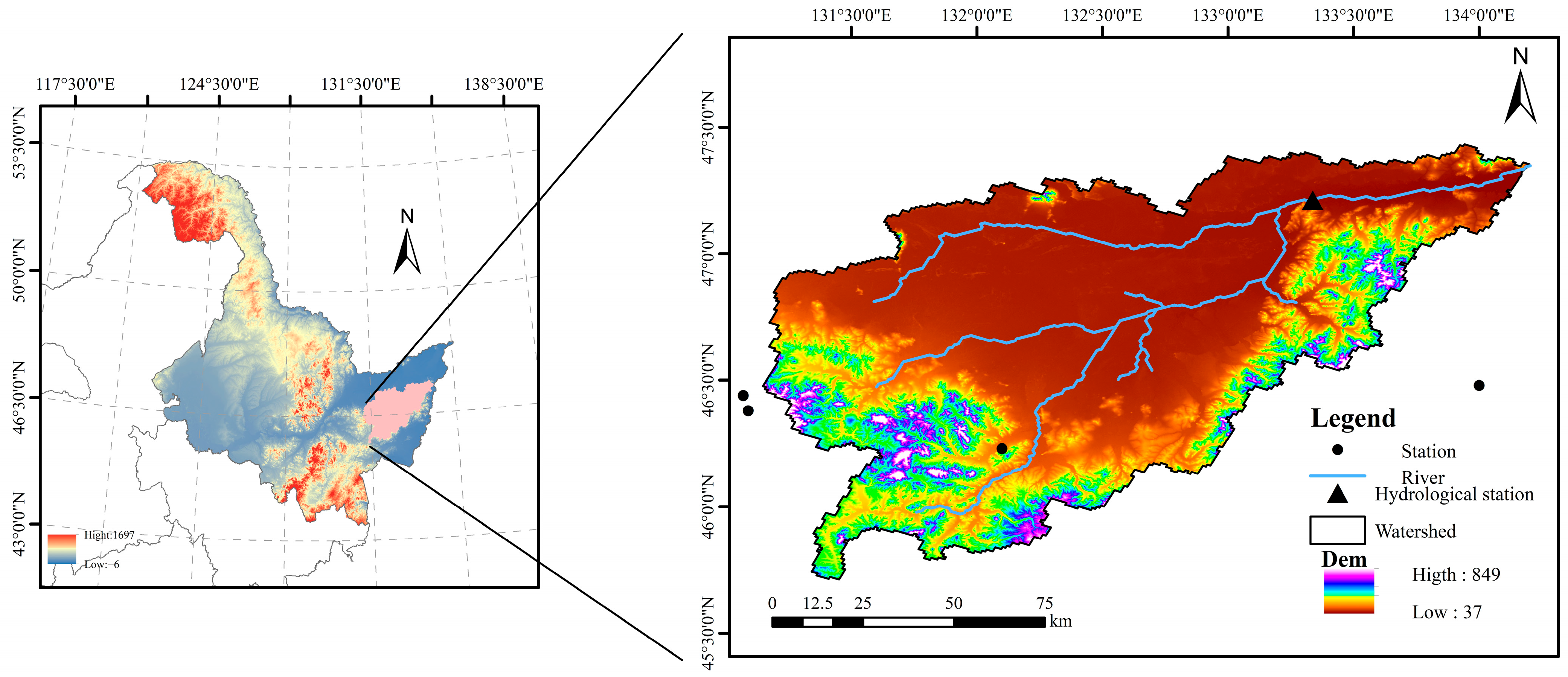
Figure 1. Distribution of water systems and hydrological stations in the Naoli River basin.
Sustainability 17 08219 g001
Figure 2. The comparison between the theoretical and empirical frequencies of various drought characteristics under different scenarios. (a) shows the comparison between the theoretical and empirical frequencies of SPAEI characteristics under different scenarios; (b) shows the comparison between the theoretical and empirical frequencies of SRI characteristics under different scenarios; (c) shows the comparison between the theoretical and empirical frequencies of SSMI characteristics under different scenarios.
Sustainability 17 08219 g002aSustainability 17 08219 g002b
Figure 3. Probability map of “and” and “or” for short- and long-term SPAEI drought characteristic variables under the SSP245 scenario.
Sustainability 17 08219 g003aSustainability 17 08219 g003b
Figure 4. Probability map of “and” and “or” for short-term and long-term SPAEI drought characteristic variables under the SSP585 scenario.
Sustainability 17 08219 g004
Figure 5. Joint occurrence probability of three-dimensional drought under the “OR” condition.
Sustainability 17 08219 g005
Figure 6. Joint occurrence probability of three-dimensional drought under the “AND” condition.
Sustainability 17 08219 g006
Table 1. Data source information [36].
Data TypeData NameYearData Source
Basic dataA dataset of multi-period remote sensing monitoring of land use in China CNLUCC2000, 2010, and 2020Chinese Academy of Sciences Center for Resources and Environmental Science and Data (https://www.resdc.cn/)
hydrological station data2020Earth Resources Data Cloud Platform (www.gis5g.com)
Natural elementASTER GDEM V3 (X1)2019Geospatial data cloud (https://www.gscloud.cn/)
slope (X2)Calculated from DEM slope
Distance from water (X3)2019OpenStreetMap
(https://www.openstreetmap.org)
Temperature/forecast (X4)2040, 2060, and 2080Chinese Academy of Sciences Center for Resources and Environmental Science and Data (https://www.resdc.cn/)
Precipitation/future precipitation (X5)CMIP6 database (https://www.nccs.nasa.gov)
Socioeconomic factorPopulation/future population (X6)2019,
2040, 2060, and 2080
Chinese Academy of Sciences Center for Resources and Environmental Science and Data (https://www.resdc.cn/)
Scientific data bank (https://cstr.cn/31253.11.sciencedb.01683)
GDP/future GDP (X7)Chinese Academy of Sciences Center for Resources and Environmental Science and Data (https://www.resdc.cn/)
Distance between government seat (city or county level) (X8 and X9)2019National Geographic Information Resources Catalog Service System (https://www.webmap.cn/)
Nature reserve (X10)2019OpenStreetMap
(https://www.openstreetmap.org)
Distance to primary, secondary, and tertiary roads (X11, X12, and X13)
Night light (X14)
Table 2. Overview of the 14 global climate patterns for CMIP 6 [36].
Pattern NameCountrySpatial ResolutionPattern NameCountrySpatial Resolution
ACCESS-CM2Australia0.25° × 0.25°EC-Earth3Europe0.25° × 0.25°
ACCESS-ESM1-5IPSL-CM6A-LR
NorESM2-LMNorwayMIROC6Japan
NorESM2-MMMIROC-ES2L
MPI-ESM1-2-HRGermanyMRI-ESM2-0
MPI-ESM1-2-LRGFDL-CM4
GFDL-ESM4
United States
INM-CM4-8RussiaCanESM5Canada
Table 3. Domain weights and transfer costs matrix under different scenarios [36].
Land Use TypeField WeightSSP245 ScenarioSSP585 Scenario
CFGWBUCFGWBU
C1111100111011
F0.671011001111011
G0.008111101111011
W0.028001110000101
B0.001111111111101
U0.075001001000001
Note: C denotes arable land, F represents forest land, G stands for grassland, U indicates urban land, B refers to bare land, and W signifies watershed. A value of 1 indicates that conversion between two land use and land cover types is possible, while a value of 0 signifies that such a conversion is not feasible.
Table 4. Drought events and drought characteristic variables in the Naoli River Basin.
ScenarioTimeSPAEISRISSMI
Event CountDurationSeverityIntensityEvent CountDurationSeverityIntensityEvent CountDurationSeverityIntensity
SSP2452025–2050223.914.271.01175.006.781.18205.406.901.10
2051–2100414.154.931.12364.725.200.99294.345.601.15
SSP5852025–2050214.485.121.06214.145.371.12214.335.151.08
2051–2100384.034.671.18335.736.161.02354.465.781.19
Table 5. AIC test results for the fitting distribution of drought characteristic variables under different time periods and types.
ScenarioTime SlotDistribution TypeAIC Value
Meteorological DroughtHydrological DroughtAgricultural Drought
DSPDSPDSP
SSP2452025–2050Gamma89.67102.518.4983.46102.0027.18100.04119.8324.66
Weibull91.94103.8911.7483.24102.4530.49100.78120.2126.90
Logistic96.79113.3511.5887.21112.6231.64106.11132.1029.22
Normal96.81114.2211.1985.50115.3333.71104.59132.0328.54
Exponential102.22105.8844.1190.72101.0741.71109.46119.2645.78
2051–2100Gamma179.90207.7813.83176.44191.659.04121.80157.1539.55
Weibull185.74211.3419.94181.76194.0718.18123.61158.5344.80
Logistic195.08227.6916.98195.26217.8310.83128.68173.3747.19
Normal199.06232.2417.53209.74239.2615.64127.15175.2548.96
Exponential204.43218.9495.78185.76192.7173.54145.20159.8768.04
SSP5852025–2050Gamma102.13112.5015.22100.19116.1422.9392.70110.1315.14
Weibull105.53113.9316.64103.11116.6024.9794.26111.3718.58
Logistic113.88129.6918.66113.41136.8526.2798.83121.0517.88
Normal122.41135.1317.00120.99143.8425.8098.14122.2918.39
Exponential106.95112.5846.25103.70114.6048.74105.59112.8347.25
2051–2100Gamma162.17176.6921.83170.70182.26−4.62157.65190.1936.80
Weibull169.53182.3830.89173.41184.61−1.25163.11193.0344.55
Logistic175.64187.5924.76184.60199.52−1.52169.34209.0542.57
Normal187.33200.9528.61184.79203.13−3.07176.45220.2545.85
Exponential182.86193.7790.02183.19188.0469.35176.62194.7584.34
Note: Bold numbers are AIC values of marginal distributions.
Table 6. Drought characteristic variables corresponding to different cumulative frequencies.
Scenario D ¯ /Month S ¯ P ¯
75%50%25%75%50%25%75%50%25%
Meteorological drought
SSP2452352.083.275.860.881.031.21
SSP5852342.303.635.600.891.091.31
Hydrological drought
SSP2452461.903.876.210.810.971.17
SSP58533.562.323.326.080.841.001.21
Agricultural drought
SSP2453472.164.139.260.740.921.42
SSP585245.52.294.016.640.851.021.35
Table 7. Conditional probability of hydrological drought under different meteorological drought scenarios.
ScenarioMeteorological Drought LevelHydrological Drought Level: 2Hydrological Drought Level: 3Hydrological Drought Level: 4Hydrological Drought Level: 5
SSP24520.180.100.040.03
30.190.120.060.04
40.190.140.090.08
50.170.150.110.17
SSP58520.190.120.060.03
30.200.150.080.05
40.210.170.100.07
50.210.190.140.12
Table 8. Conditional probability of agricultural drought under different meteorological drought scenarios.
ScenarioMeteorological Drought LevelAgricultural Drought Level: 2Agricultural Drought Level: 3Agricultural Drought Level: 4Agricultural Drought Level: 5
SSP24520.190.120.060.03
30.200.150.080.05
40.210.170.110.07
50.210.190.140.12
SSP58520.200.110.040.02
30.230.150.080.05
40.220.180.120.10
50.170.180.150.24
Disclaimer/Publisher’s Note: The statements, opinions and data contained in all publications are solely those of the individual author(s) and contributor(s) and not of MDPI and/or the editor(s). MDPI and/or the editor(s) disclaim responsibility for any injury to people or property resulting from any ideas, methods, instructions or products referred to in the content.