Article

Optimized Extrapolation Methods Enhance Prediction of Elsholtzia densa Distribution on the Tibetan Plateau

1
Institute of Plant Protection, College of Agricultural and Forestry Sciences, Qinghai University, Xining 810005, China
2
Qinghai Academy of Agricultural and Forestry Sciences, Xining 810005, China
*
Author to whom correspondence should be addressed.
Sustainability 2025, 17(18), 8206; https://doi.org/10.3390/su17188206
Submission received: 8 July 2025 / Revised: 2 September 2025 / Accepted: 4 September 2025 / Published: 11 September 2025

Abstract

Species distribution models (SDMs) grapple with uncertainty. To address this, a parameter-optimized MaxEnt model was used to predict habitat suitability for Elsholtzia densa, a predominant agricultural weed on the Tibetan Plateau. Through multiparameter optimization with 149 occurrence points and three climate variable sets, we systematically evaluated how the three MaxEnt extrapolation approaches (Free Extrapolation, Extrapolation with Clamping, No Extrapolation) influenced model outputs. The results showed the following: (1) Model optimization using the Kuenm R package version (1.1.10) identified seven critical bioclimatic variables (Feature Combinations = LQTH, Regularization Multipliers = 2.5), with optimized models demonstrating high accuracy (Area Under Curve > 0.9). (2) Extrapolation approaches exhibited negligible effects on variable selection, though four bioclimatic variables “bio1 (annual mean temperature)”, “bio12 (annual precipitation)”, “bio2 (mean diurnal range)”, and “bio7 (temperature annual range)” predominantly drove model predictions. (3) Current high-suitability areas are clustered in the eastern and southern regions of the Tibetan Plateau, and with Free Extrapolation yielding the broadest current distribution. Climate change projections suggest habitat expansion, particularly under conditions of No Extrapolation. (4) Multivariate Environmental Similarity Surface (MESS) and Most Dissimilar Variable (MoD) are not affected by the extrapolation method, and extrapolation risk analyses indicate that future climate anomalies are mainly concentrated in the western and southern parts of the Tibetan Plateau and that future warming will further increase the unsuitability of these regions. (5) Variance analysis showed that the extrapolation methods did not significantly affect the 10-replicate results but influenced the parameter and emission scenarios, with No Extrapolation methods showing minimal variance changes. Our findings validate that multiparameter optimization improves species distribution model robustness, systematically characterizes extrapolation impacts on distribution projections, and provides a conceptual framework and early warning systems for agricultural weed management on the Tibetan Plateau.

1. Introduction

Climate plays a key role in the distribution of species on Earth, affecting many aspects of plant growth and development [1]. It also significantly impacts the geographical distribution of plant species [2]. Over the past 100 years, global surface temperature has risen by 0.85 °C due to global warming [3]. Continued climate warming has led to plant populations responding differently [4]. Surface temperatures are also expected to continue rising towards the end of the 21st century [5]. Because of its unique geographic location and topographic features, the Tibetan Plateau is highly vulnerable to climate warming [6]. While climate change affects the growth and development of vegetation on the plateau, changes in the state of the vegetation can also trigger changes in the heat source of the plateau region, which in turn affects the regional and global climate [7].
Species distribution models (SDMs) are important tools for modeling, analyzing, and predicting the geographical distribution of species’ habitat [8]. They are used to predict the potential distribution areas of a species by combining species distribution and environmental data with geographic maps. Using specific algorithms, they estimate ecological niches and express species’ habitat preferences probabilistically [9]. To adhere to contemporary modeling standards, we followed best-practice guidelines for SDMs [10,11], which emphasize the importance of addressing sampling bias, model evaluation, and uncertainty quantification. SDMs have emerged as critical tools for assessing the impacts of climate change on the potential distribution of species. Common models include the Bioclimatic Analysis System (Bioclim), Genetic Algorithm for Rule-set Production (GARP), Ecological Niche Factor Analysis (ENFA), Random Forest (RF), and Maximum Entropy (MaxEnt) models [12]. Among SDMs, the MaxEnt model demonstrates strengths, including high predictive precision, reduced computational time, consistent results, and lower sample size requirements [13], with the added capability of making reliable inferences and predictions even when handling incomplete datasets [14]. The MaxEnt model is a widely used machine learning method for species distribution modeling. It predicts species distributions under varying environmental conditions by maximizing entropy and incorporating environmental factors [15,16]. Retaining the default algorithmic configuration can lead to significant overfitting risks and unwarranted model complexity, ultimately compromising prediction reliability and diminishing its utility in habitat suitability projections [5]. Adjusting key parameters such as the regularization multiplier (RM) and feature classes (FCs) in MaxEnt models using the Kuenm package in R programming language enables refined model calibration, enhancing predictive transferability and ecological realism to meet the specific requirements of different species [17], and the optimized MaxEnt model has been widely applied in fields such as invasive species risk assessment [18] and harmful weed distribution prediction [19]. Research conducted by Scherrer [20] demonstrated that while substantial progress has been made in understanding the effects of covariates, including sample size, SDM algorithm selection, and variable filtering, on MaxEnt’s predictive performance, critical gaps persist regarding their impact on the spatial configuration of model outputs, particularly in the context of projective extrapolation under novel environmental conditions. This methodological dimension remains underexplored in the contemporary SDM literature.
Selecting appropriate extrapolation strategies can significantly enhance the practicality and reliability of a model. Each extrapolation approach has its own applicable scenarios, advantages, and disadvantages. The choice of strategy should be based on the research objectives and data characteristics. In MaxEnt models, the accuracy and reliability of the extrapolation are key factors that affect the performance of the final model, and different extrapolation strategies are used to deal with problems that may arise when model predictions are outside the context of the training data. Specifically, MaxEnt uses three extrapolation methods [21]. (1) E (Free Extrapolation): which can freely predict areas beyond the environmental range of the training data, and the model predicts the distribution of species outside the range of environmental conditions based on the distribution pattern constructed from the training data. Free extrapolation does not impose any restrictions, allowing the model to predict the distribution of a species within a completely unknown environmental range, making it suitable for exploring new environmental regions where the species may exist. (2) EC (Extrapolation and Clamping): This method not only extrapolates but also uses a “clamping” technique to constrain the results of the extrapolation. This method combines Extrapolation with Clamping to mitigate inaccuracies from the Free Extrapolation. It restricts predictions in extreme environmental conditions beyond the training data, enhancing reliability. (3) NE (No Extrapolation): The MaxEnt model strictly limits its predictions to the environmental range of the training data, and the model does not make any predictions for areas beyond the environmental conditions of the training data. This model predicts species only within a known environmental range, completely avoiding the risk of extrapolation, and is the most conservative extrapolation strategy for predicting species distributions based on known environmental data.
Elsholtizia densa Benth. (Figure 1) is a plant belonging to the genus Elsholtzia within the family Labiatae [22]. It is primarily distributed in Shaanxi, Sichuan, Yunnan, Gansu, Qinghai, Tibet, and the Xinjiang provinces of China, growing along forest edges, high mountains, meadows, under forests, along rivers, and on slopes at elevations of 2800–4100 meters [23]. It is also found in Afghanistan, Pakistan, Nepal, India, and Russia [23]. It displays indeterminate growth, concurrent flowering–fruiting cycles, and progressive seed shattering, which jeopardizes agronomic productivity by interfering with crop phenology and yield components [24]. This species has emerged as a pernicious weed in agroecosystems across the Qinghai-Tibetan Plateau [22]. Concurrently, Elsholtzia densa produces abundant senescent plant tissues that decompose and release allelopathic compounds into the soil, which alters the rhizosphere biochemical environment and disrupts plant–microbe defense symbioses, inducing phytotoxic effects that directly impede vegetative growth through secondary metabolite-mediated interactions, thereby exacerbating ecological degradation in the Qinghai-Tibetan Plateau agroecosystems through allelopathic cascade effects [25]. Consequently, analyzing climate-driven distribution shifts of Elsholtizia densa across the Qinghai-Tibetan Plateau is essential for establishing critical baselines to predict invasion trajectories under projected climatic scenarios. This analysis will also enable dynamic monitoring frameworks to track its spatial–temporal dispersal patterns and facilitate the formulation of effective conservation and management strategies.
While parameter optimization enhances the internal validity of SDMs, their predictive robustness under novel environments—a process inherently reliant on extrapolation—remains a critical methodological challenge. Different extrapolation strategies embody distinct philosophical assumptions about species’ ecological niches: Free Extrapolation assumes niche conservatism into novel conditions, Extrapolation with Clamping introduces mechanistic constraints to mitigate extreme predictions, and No Extrapolation adopts a strictly interpolative, conservative approach. However, the interaction between model optimization and these extrapolation methods is poorly understood, leading to uncertainties in projection reliability. We aim not only to forecast its distributional shifts under climate change but also to critically assess the theoretical implications of extrapolation choices on model outcomes. Our research specifically seeks to (1) predict potentially suitable habitats for Elsholtzia densa under three extrapolation modes, (2) analyze the extrapolation risk of the models, and (3) use analysis of variance for different numbers of repetitions, different parameters, and different emission scenarios in the MaxEnt model. This conceptual framework provides a robust basis for interpreting projection uncertainties and offers insights into the ecological realism of different modeling approaches.

2. Materials and Methods

2.1. Sources of Distribution Data

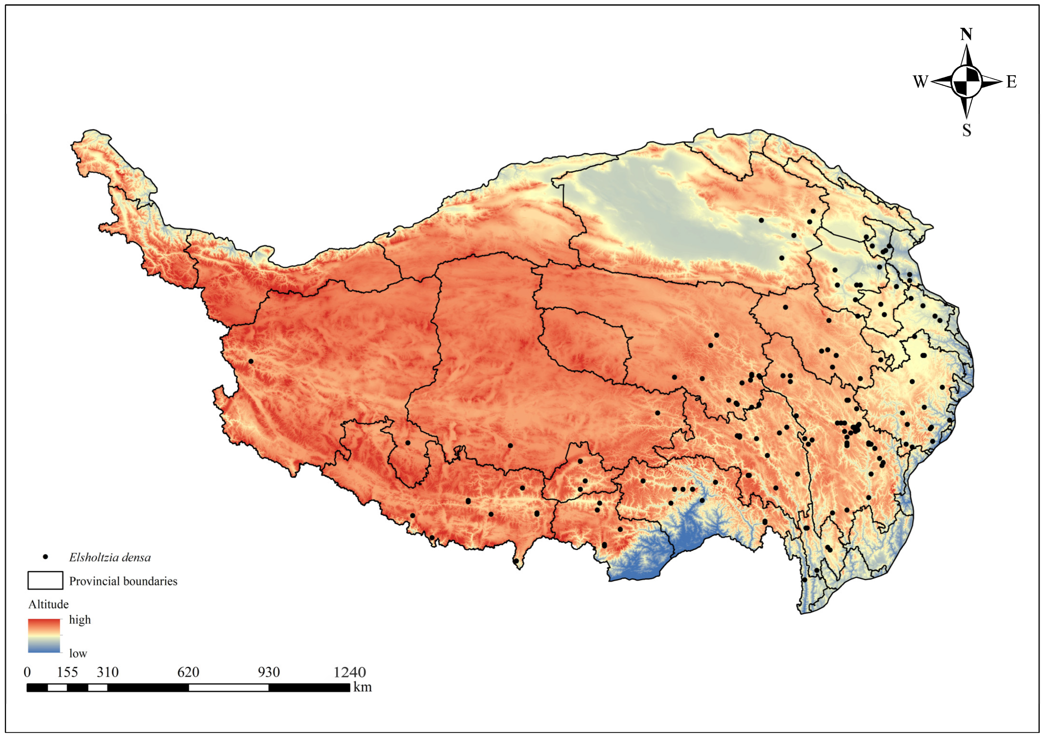
Distribution data of Elsholtzia densa were collected through two approaches: (1) the field investigations (Table 1) show that the altitude ranges from 1790 to 3316 m and (2) retrieval of precise georeferenced occurrence records from the Global Biodiversity Information Facility (GBIF, https://doi.org/10.15468/dl.b8sx2a, accessed on 14 April 2024) [26] and the Chinese Virtual Herbarium (CVH, https://www.cvh.ac.cn/index.php, accessed on 14 April 2024), and the corresponding DOI link for Elsholtzia densa in the GBIF search is https://doi.org/10.15468/dl.b8sx2a, accessed on 14 April 2024. To mitigate sampling bias, minimize spatial autocorrelation, and avoid model overfitting, the distribution data of Elsholtzia densa were spatially rarefied using ENMTools (version 1.1.2) to retain only one occurrence record per 5 × 5 km grid cell [27], yielding a final dataset of 149 georeferenced occurrences (Figure 2). The filtered records are compiled into a CSV file, structured with the species name, longitude, and latitude fields for downstream analyses. In constructing the species distribution model for this study, the distribution data for Elsholtzia densa only included the Qinghai–Tibet Plateau region of China (Figure 2). Although this species is also distributed in Hebei and Shanxi provinces in China, as well as in Pakistan, Nepal, India, and other regions, with distribution data available (GBIF, https://doi.org/10.15468/dl.b8sx2a, accessed on 14 April 2024), this study focuses on the potential distribution at the regional scale of the Qinghai–Tibet Plateau. This is to avoid the interference of large-scale environmental heterogeneity on local predictions.
To optimize the model training efficacy and predictive performance, the occurrence data of Elsholtzia densa across the Qinghai–Tibet Plateau were subjected to randomized partitioning using the kuenm_occsplit package in R. This process involved a two-stage split: primary partitioning into a 95% training set and a 5% independent test set, followed by secondary partitioning of the training subset into 75% model calibration data and 25% validation data.

2.2. Environmental Variable Data and Screening

The climatic datasets were derived from 19 bioclimatic variables obtained through the WorldClim platform (version 2.1, https://www.worldclim.org/, accessed on 8 October 2023), encompassing the historical baseline (1970–2000s) and projections for the 2070s (2061–2080). Three emission scenarios under the Representative Concentration Pathways framework (RCP2.6, RCP4.5, and RCP8.5) were adopted, corresponding to low, medium, and high radiative forcing trajectories [29]. We conducted Pearson correlation analyses in R (version 4.4.2) to resolve multicollinearity issues among the 19 bioclimatic variables, retaining the most representative variable when pairwise correlations between environmental predictors surpassed 0.8 to enhance model interpretability [30]. We employed the R package “Kuenm” to conduct simultaneous optimization of three environmental variable (Table 2) sets to obtain robust climate predictors: the first group of bioclimatic factors did not utilize Pearson’s correlation test and comprised 19 factors (bio1–bio19); the second group employed Pearson’s correlation test and, following a screening process, included 7 factors (bio1, bio2, bio3, bio7, bio12, bio14, bio15); the third group also applied Pearson’s correlation test; however, to prevent overlap with the factors in the second group, it resulted in the selection of 8 distinct factors (bio2, bio3, bio4, bio8, bio9, bio13, bio15, bio17).

2.3. MaxEnt Parameter Setting and Accuracy Evaluation

The R package “kuenm” was implemented to optimize feature combinations (FCs) and regularization multipliers (RMs) in MaxEnt models. Model selection was guided by the principle of parsimony to enhance model transferability—a critical aspect for extrapolation into novel climates. We used the corrected Akaike Information Criterion (AICc) for small sample sizes, which penalizes model complexity, to identify the model that best explains the data with the fewest parameters. The model with the lowest AICc value was selected as optimal, as it is theoretically less prone to overfitting and thus expected to demonstrate more reliable predictive performance when extrapolating [31]. Combinatorial validation was conducted by systematically testing the RM values (0–4 in 0.1 increments) against FC(LQPTH). The definitive model was determined using three criteria: statistical significance, omission rate below 5%, and the corrected Akaike Information Criterion (delta AICc) < 2 (with delta AICc = 0 prioritized) [17].

2.4. Model Extrapolation Patterns

We implemented ten bootstrap replicates using activated jackknife validation. We utilized 75% of the distribution points as the training set to fit the model, while the remaining 25% were used to test the model. Subsequently, we employed the kuenm_mod function to predict suitable areas based on the three selected bioclimatic factors and optimized parameters [32]. We implemented all three extrapolation approaches available in MaxEnt: Free Extrapolation (E), Extrapolation with Clamping (EC), and No Extrapolation (NE).

2.5. Model Accuracy Assessment and Habitat Suitability Classification

Predictive performance of the model was assessed using Receiver Operating Characteristic (ROC) analysis, with model efficacy quantified through Area Under the Curve (AUC) calculations [33]. AUC ranges from 0 to 1, with thresholds indicating credibility: 0.6–0.7 (low), 0.7–0.8 (moderate), 0.8–0.9 (high), and >0.9 (excellent) [34].
Habitat suitability for Elsholtizia densa was categorized into four tiers using manual reclassification in ArcGIS 10.8: high suitability (0.6–1.0), moderate suitability (0.4–0.6), low suitability (0.2–0.4), and unsuitable (0.0–0.2), with area statistics calculated for each climate scenario [35].
Climate-driven habitat dynamics were categorized as follows: persistently unsuitable, newly suitable area (new suitability in ≥1 GCM), lost suitable area (lost suitability in ≥1 GCM), and persistently suitable across all climate projections [36]. Persistently unsuitable areas remain unsuitable in both current and future periods; newly suitable areas transition from unsuitable to suitable; lost suitable areas shift from suitable to unsuitable; stable suitable areas maintain suitability across time periods.

2.6. Multivariate Environmental Similarity Surface and Most Dissimilar Variable

MESS (Multivariate Environmental Similarity Surface) measures climatic congruence between future projections and baseline conditions. Negative scores (≥1 variable beyond reference range) indicate extrapolation risk, whereas positive values reflect environmental consistency. Maximum similarity = 100 and negative values denote substantial divergence. MESS values were stratified into five categories: S < 0, 0 ≤ S < 20, 20 ≤ S < 40, 40 ≤ S < 60, and S ≥ 60. The Most Dissimilar Variable (MoD) refers to the environmental variable exhibiting the lowest multivariate similarity, indicating the highest degree of abnormality, at a specific point, and this environmental variable may be a factor influencing changes in the species’ habitat [37].

2.7. Integrated Model Uncertainty Analysis

Model extrapolation risk was evaluated using the kuenm_mmop function (10% threshold), producing MOP rasters (0–1 scale), where 0 denotes high environmental dissimilarity, and higher values reflect greater similarity. Elevated extrapolation risk indices were correlated with improved habitat suitability and enhanced environmental analog assessments of ENM outputs [38].
Concurrently, discrepancies among the ten model replicates were analyzed using R’s kuenm_modstats function, where greater variation ranges denote reduced model replicability (lower reliability) and smaller ranges indicate higher consistency (enhanced credibility).
Further comprehensive uncertainty assessment was conducted via R’s kuenm_modvar function to analyze (1) variance patterns across 10 model replicates under different temporal scenarios, with higher variance indicating greater projection uncertainty; (2) parameterization impacts on model outputs; and (3) emission scenario effects (RCP2.6, RCP4.5, RCP8.5) quantified through comparative variance analysis where increased variance reflects stronger climate forcing impacts.

3. Results

3.1. Model Parameter Optimization

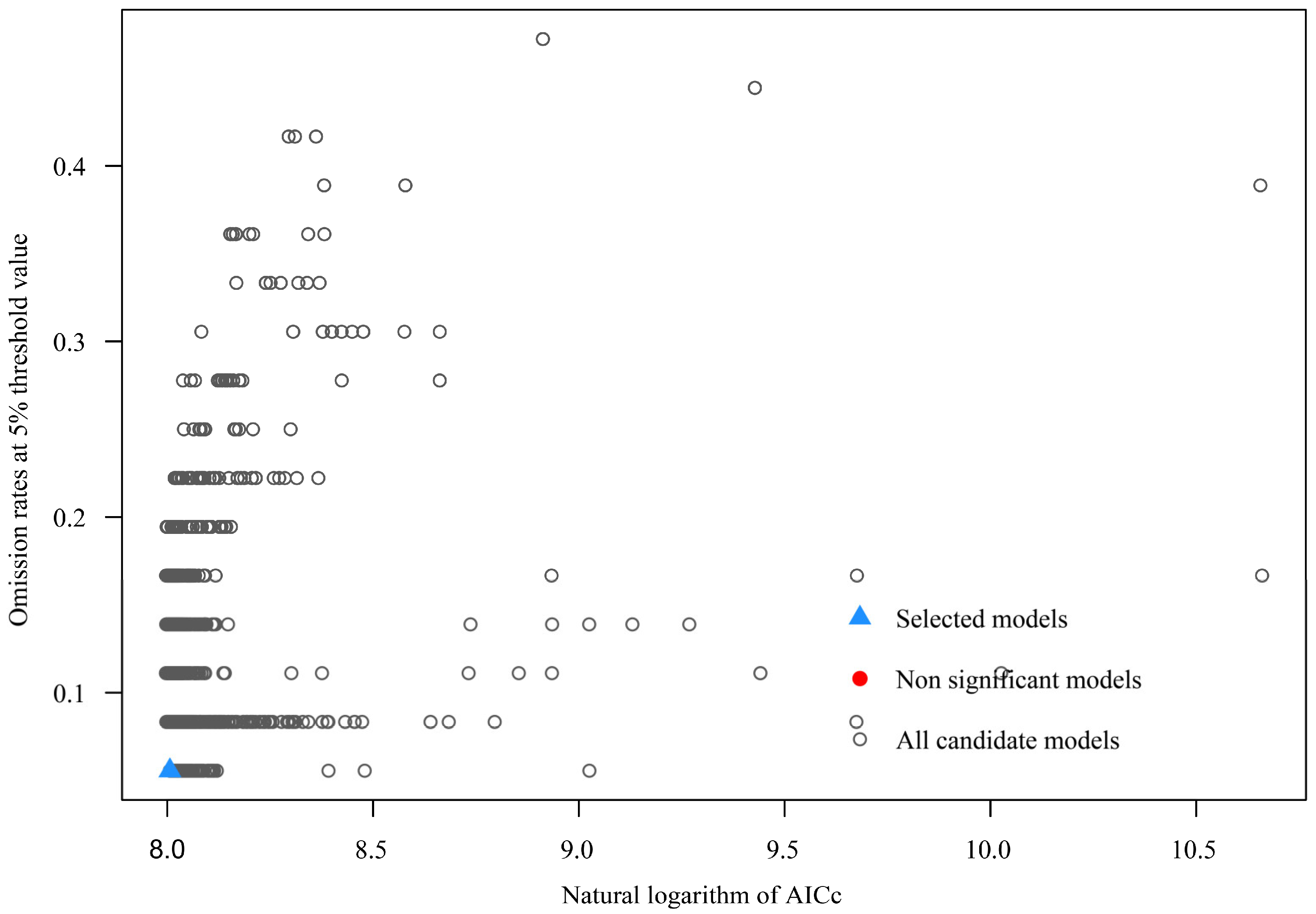
The Set2 parameterization included seven environmental factors (bio1, bio2, bio3, bio7, bio12, bio14, bio15), and combinations (FC) =LQTH and regularization multipliers (RMs) = 2.5 showed optimal performance (ΔAICc = 0) among 3720 model candidates (Figure 3, Table 3), indicating enhanced model transferability between calibration and projection domains with effective overfitting control. The mean AUC values of three extrapolation outcomes (E, EC, and NE) consistently exceeded 0.9 through 10 bootstrap iterations, validating the model’s robustness for habitat suitability prediction of Elsholtzia densa.

3.2. Dominant Environmental Determinants

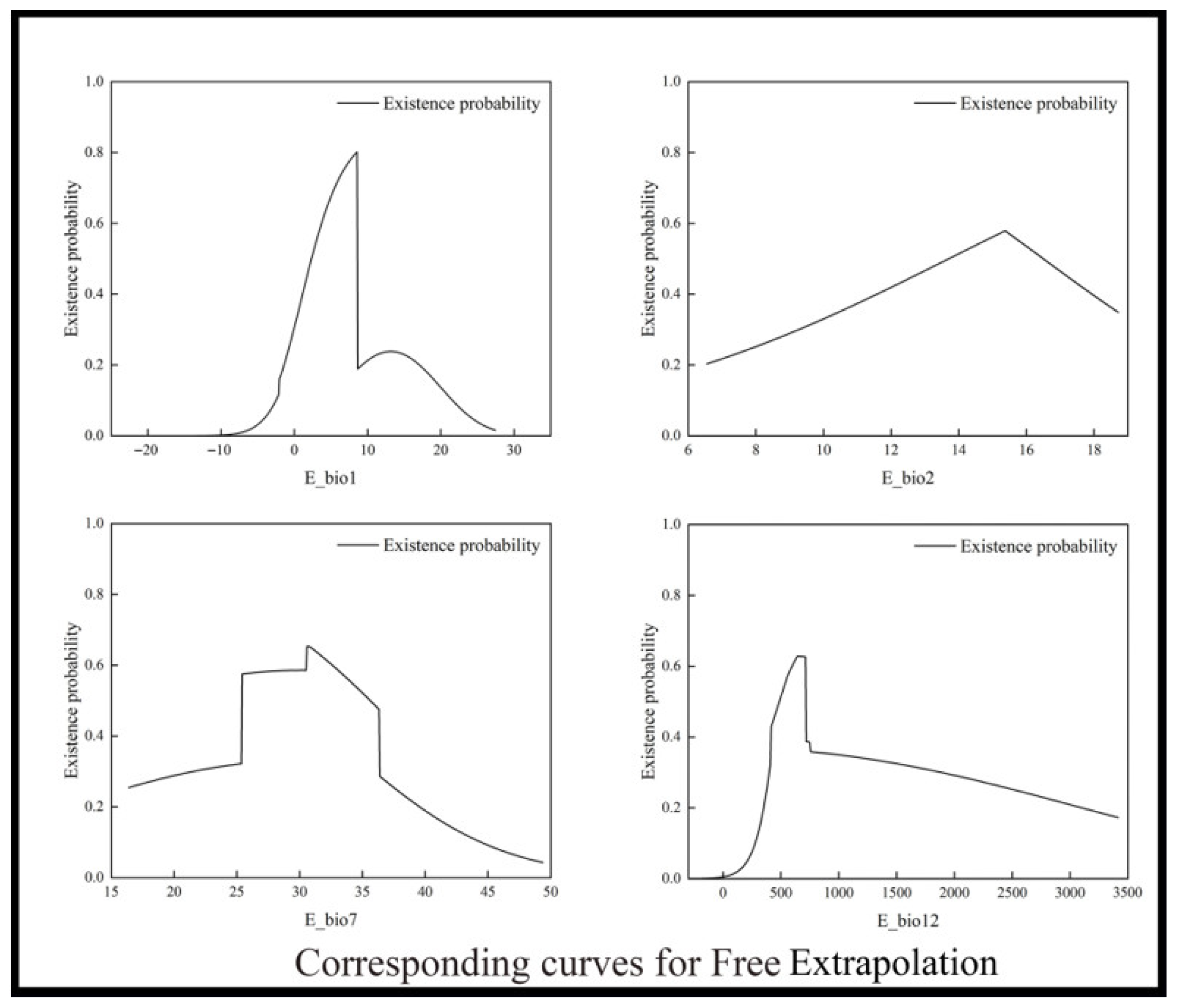
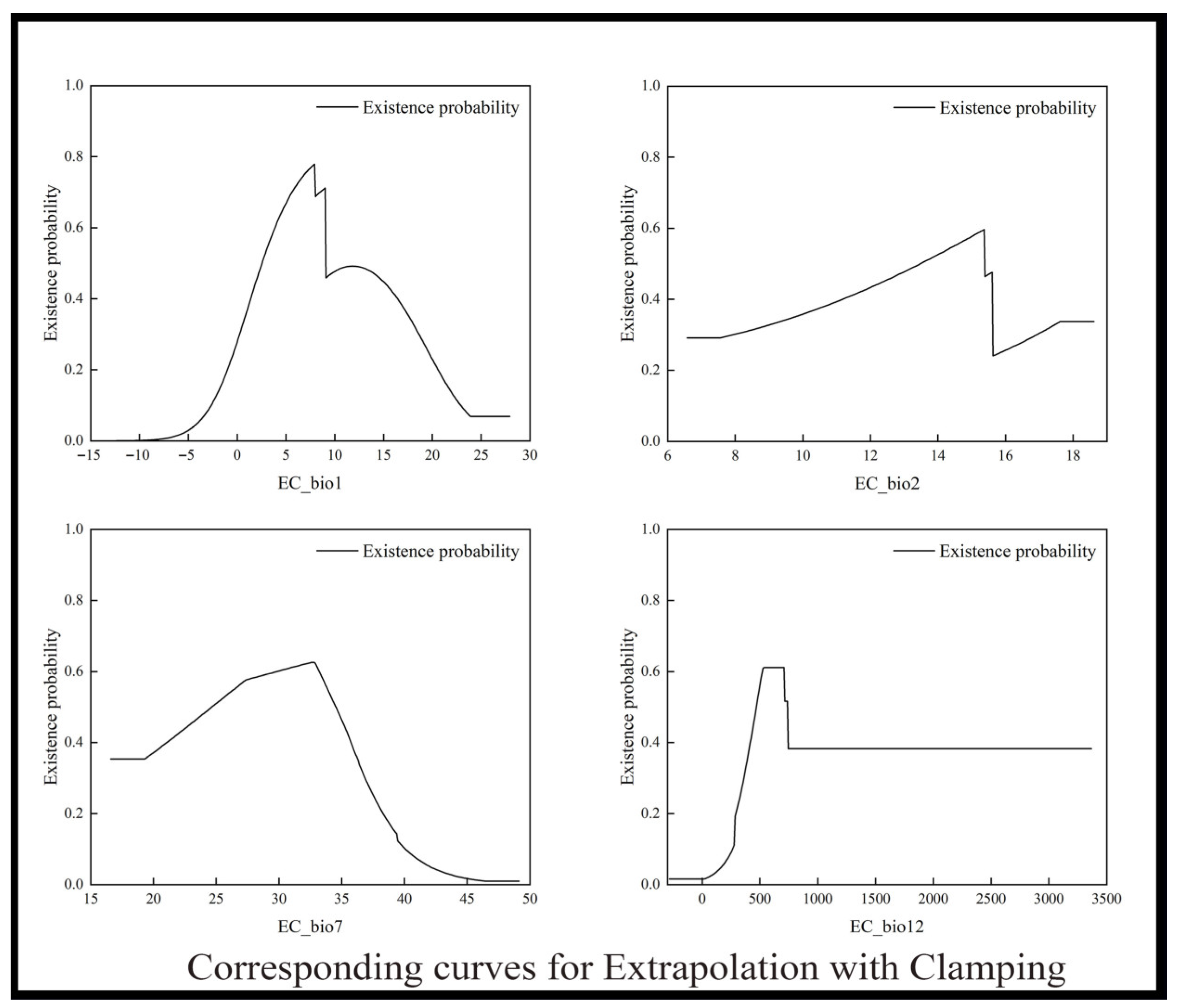
The contribution rates of each environmental variable were determined using the knife-cut method, and the factors were ranked based on their contribution rates. Factors with cumulative contribution rates exceeding 90% were identified as dominant environmental factors. The results derived from the three extrapolation models indicate that, according to the prediction results of the response curves in the MaxEnt model, the four environmental factors with the highest contribution rates to the distribution of dense-flowered hyssop are bio1 (annual average temperature), bio12 (annual precipitation), bio2 (monthly average diurnal temperature difference), and bio7 (annual temperature range). The total contribution rate of these four environmental factors exceeds 90% (E method: 95.8%, EC method: 94.4%, NE method: 94.4%), effectively reflecting the selection of suitable habitats. It is noteworthy that different extrapolation methods can influence the contribution rate of individual environmental factors.
Single-factor response curves represent different models, i.e., models created using only the corresponding variable, reflecting the correlation between predicted suitability and the selected variable. A threshold value is typically set at 0.5, serving as a general boundary to distinguish between suitable and unsuitable conditions. As shown in Figure 4, Figure 5 and Figure 6, the response curves for the suitability probability of Elsholtzia densa to environmental factors mostly exhibit a single-peak pattern. The applicability of key environmental variables under different extrapolation methods (E, EC, NE) is summarized in Table 4.
We inferred from observing the response curve that different extrapolation methods caused non-significant variations in environmental determinants but modulated probability extremes: E showed increasing or decreasing trends, EC stabilized both extremes, and NE nullified probability thresholds.

3.3. Comparison of Suitable Areas for Different Periods Under Model Extrapolation

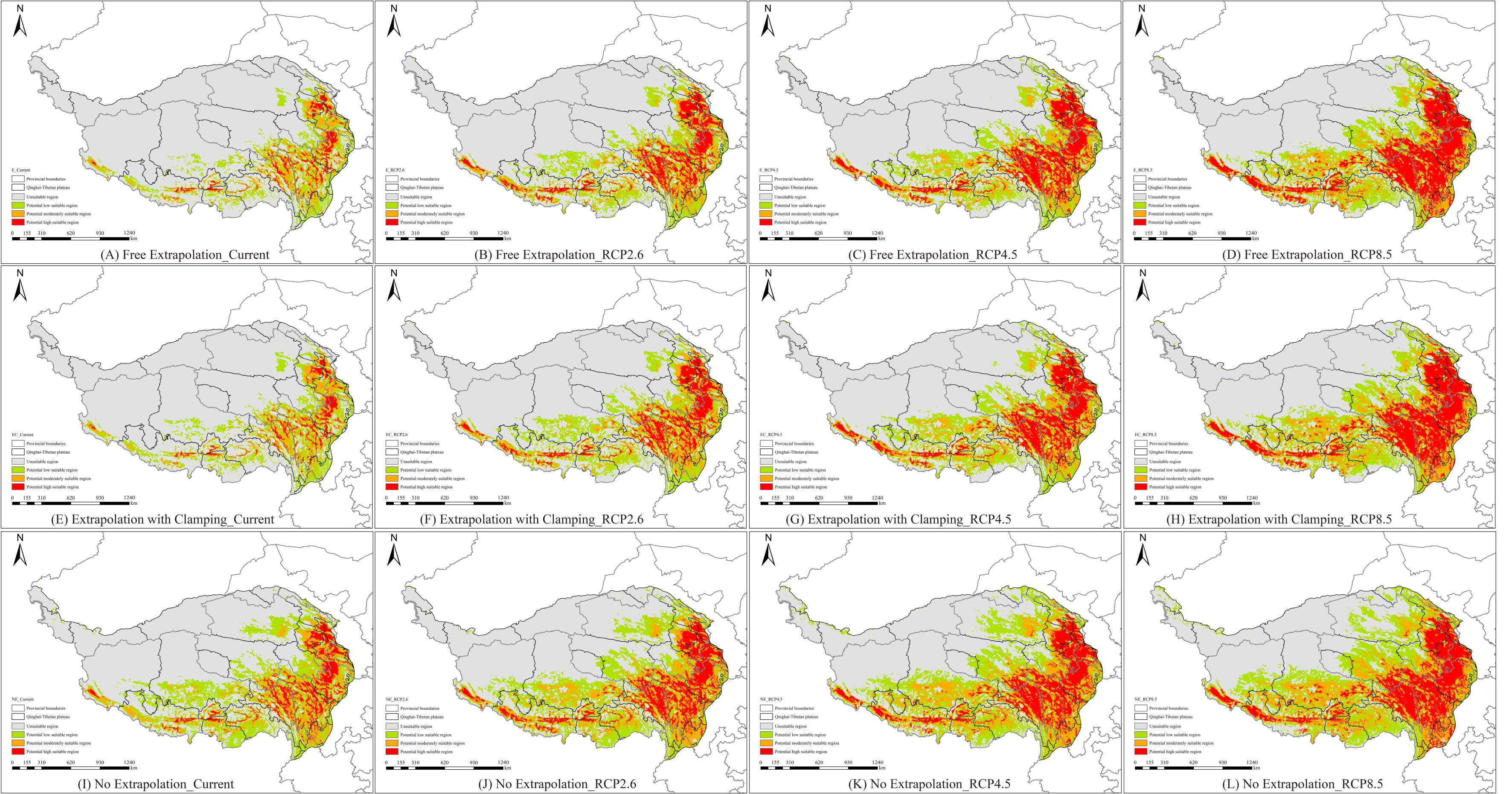
Consistent with the theoretical constraint of the method, we compared the impacts of different extrapolation methods and climate scenarios on suitable habitats of Elsholtzia densa on the Qinghai–Tibet Plateau (Figure 7). Under the current climatic conditions, suitable areas are concentrated in the eastern and southern plateaus, primarily covering Qinghai, Gansu, Sichuan, and Tibet. Free Extrapolation (E) projected the largest suitable area (56.26 × 10⁴ km2, 22.05%), followed by Extrapolation with Clamping (EC) (59.59 × 10⁴ km2, 23.36%), and No Extrapolation (NE) yielded the smallest area (59.08 × 10⁴ km2, 23.16%).
As shown in Table 5, with increasing greenhouse gas concentrations significantly affecting the distribution of Elsholtzia densa, the potential suitable area for Elsholtzia densa expanded significantly under the three future climate scenarios and mainly shifted to the central Tibetan Plateau. The distribution of Elsholtzia densa is becoming increasingly widespread, with a trend towards an increase in the current suitable habitat area. In particular, under the RCP8.5 scenario, the increase in the area of the high suitability zone under all extrapolation methods exceeded 25 × 104 km2, with the trend of the increase reaching a maximum of 37.07 × 10⁴ km2. Under the future climate scenarios, different extrapolation methods had different effects on the area of Elsholtzia densa, and the total area of the suitable zone was as follows: No Extrapolation > Extrapolation and Clamping > Extrapolation. It was also found that under the No Extrapolation approach, Elsholtzia densa had the greatest trend of growth in potential suitable areas, which increased by 67.43 × 10⁴ km2 under the RCP8.5 scenario, an increase of 13.78 × 10⁴ km2 and 4.11 × 10⁴ km2 compared with the E and EC approaches, respectively.

3.4. Spatial Pattern Changes of Potential Habitats Under Future Climate Scenarios

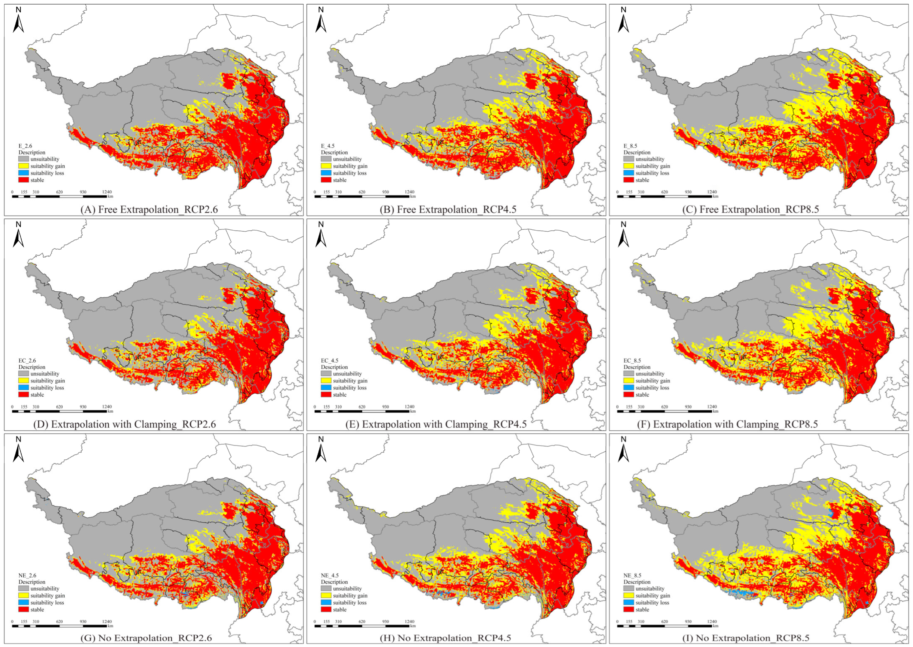
Comparative analysis of the spatial pattern of potentially suitable areas for Elsholtzia densa under the RCP2.6, RCP4.5, and RCP8.5 climate scenarios from 2061 to 2080 (Figure 8) showed that the loss of suitable areas for Elsholtzia densa did not change significantly and that the expansion area of Elsholtzia densa gradually increased with the intensification of the GHG emission scenarios from RCP2.6 to RCP8.5, especially under the higher emission scenario (RCP8.5).
As shown in Table 6, under different extrapolation methods, the model performs extrapolation under the E method, and the stable suitable area retained is the largest, the distribution of the area of suitable habitat for Elsholtzia densa under the extrapolation of the E method for the three future climate scenarios (RCP2.6, RCP4.5, and RCP8.5) showed that the retained suitable area was 81.07 × 10⁴ km2, 81.03 × 10⁴ km2, and 81.10 × 10⁴ km2. Under the NE method, the model does not perform extrapolation, and the stable suitable area retained is the smallest. Under the EC method, the model contracts during the extrapolation process, and the stable suitable area retained is between the E and NE methods.
Under future climate change, the expansion of Elsholtzia densa is projected to initiate primarily in the central Qinghai–Tibet Plateau, including Nagqu City, Golmud City, Yushu Tibetan Autonomous Prefecture, Golog Tibetan Autonomous Prefecture, and Haixi Mongol and Tibetan Autonomous Prefecture. In these regions, integrated management strategies—combining agricultural practices, chemical control, and ecological regulation—should be implemented to maintain its population density below the economic threshold. As greenhouse gas emissions intensify, further expansion is anticipated into southern areas such as Nyingchi City, Shannan City, and Shigatse City, as well as northern regions including Zhangye City and Haibei Tibetan Autonomous Prefecture. These areas should establish enhanced routine surveillance and early warning systems, with focused monitoring of high-risk zones to prevent further invasion and spread into agricultural lands.
Under the NE method, the expansion zone is the largest; under the three future climate scenarios (RCP2.6, RCP4.5, RCP8.5), the expanded suitable areas for dense-flowered fragrant mint are 30.11 × 10⁴ km2, 48.09 × 10⁴ km2, and 66.88 × 10⁴ km2, respectively. Under the E method, the expansion zone is the smallest; under the EC method, the expansion zone remains between the E and NE methods.

3.5. Multivariate Environmental Similarity Surface and Most Dissimilar Variable Analysis

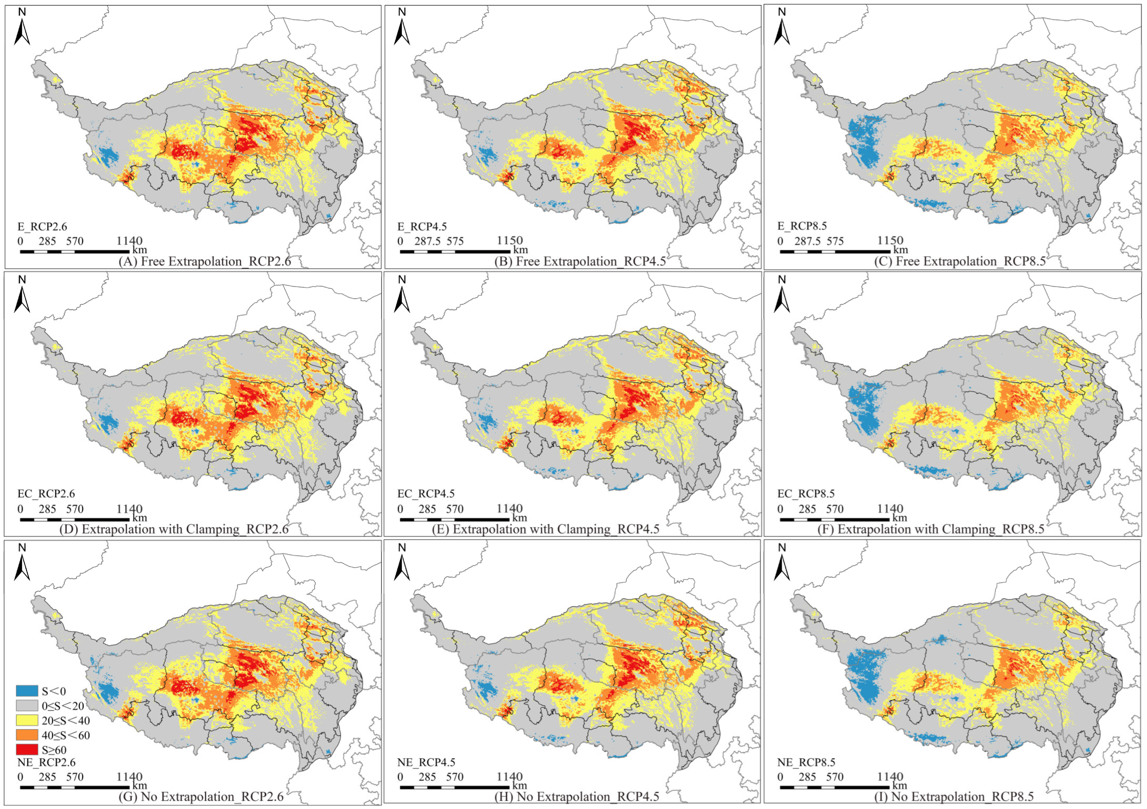
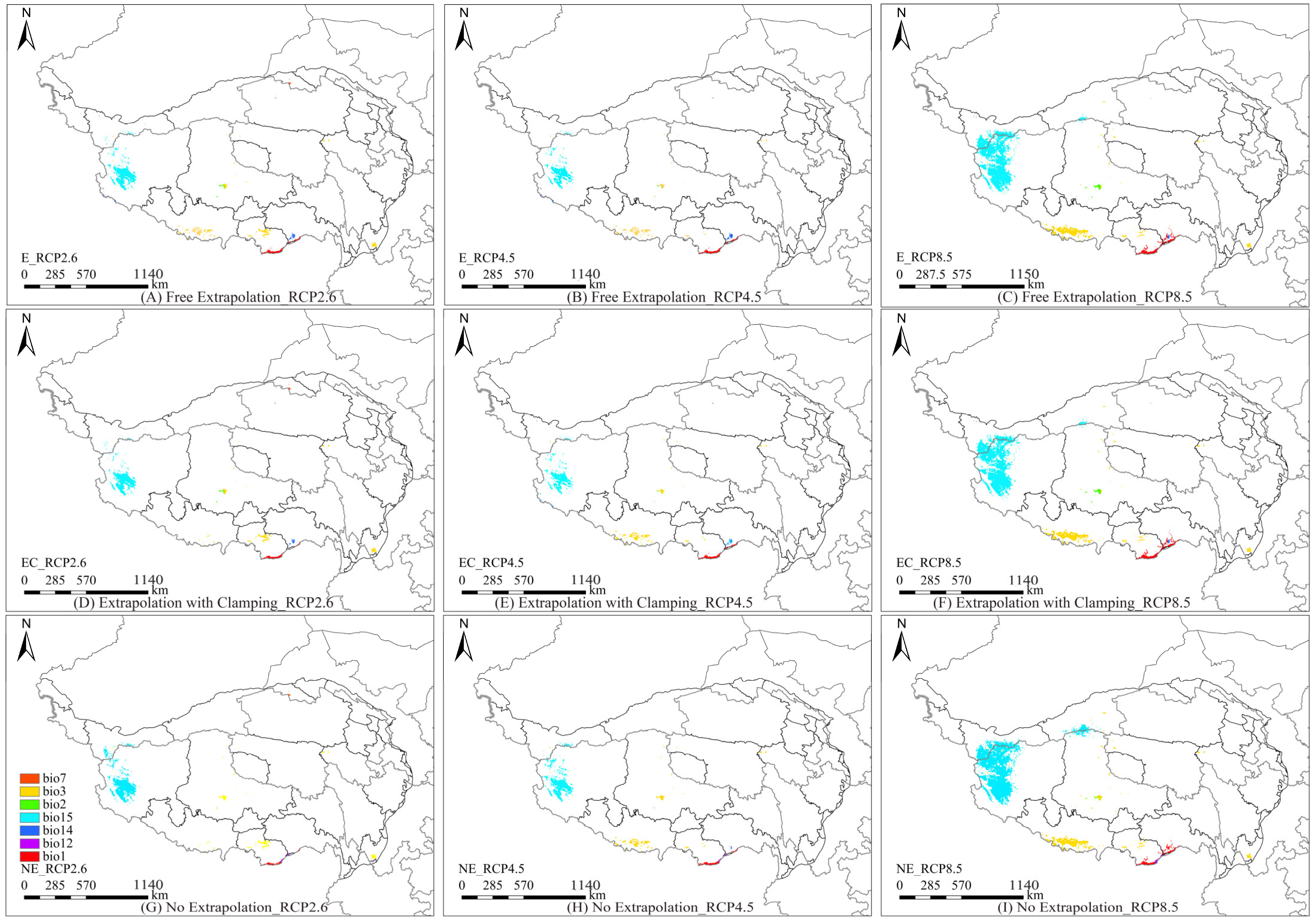
The MESS (Figure 9) and MoD (Figure 10) analyses showed negligible extrapolation effects. Significant climate anomalies (MESS < 0) emerged in Ngari Prefecture and Shannan City, with bio15 identified as the primary divergent variable under RCP2.6. The core plateau regions (Nagqu, Golmud, and Yushu) maintained high environmental analogs (MESS > 60), whereas transitional edges exhibited moderate variability (MESS 0–20) on the Tibetan Plateau. Critical divergence zones (MESS < 0) emerged in western Ngari and Shannan, signifying non-analogous climatic conditions. Under elevated emissions, non-analog climates (MESS < 0) expanded by 23.7% into Hotan and Shigatse, where bio3 and bio1 emerged as key divergent variables reflecting shifting climate constraints.
MoD analysis (Figure 10) identified bio15 as the primary anomaly driver in Ngari and Hotan under RCP2.6, with bio3 affecting Shigatse and Nagqu, and bio1 dominating southern Nanshan. Emission intensification expanded the influence of the MoD; bio15 extended to the Bayingolin Mongol Autonomous Prefecture and northern Nagqu, bio3 penetrated southern Shigatse, and bio1 reached Nyingchi’s southern territories.

3.6. Model Extrapolation Risk Comparison

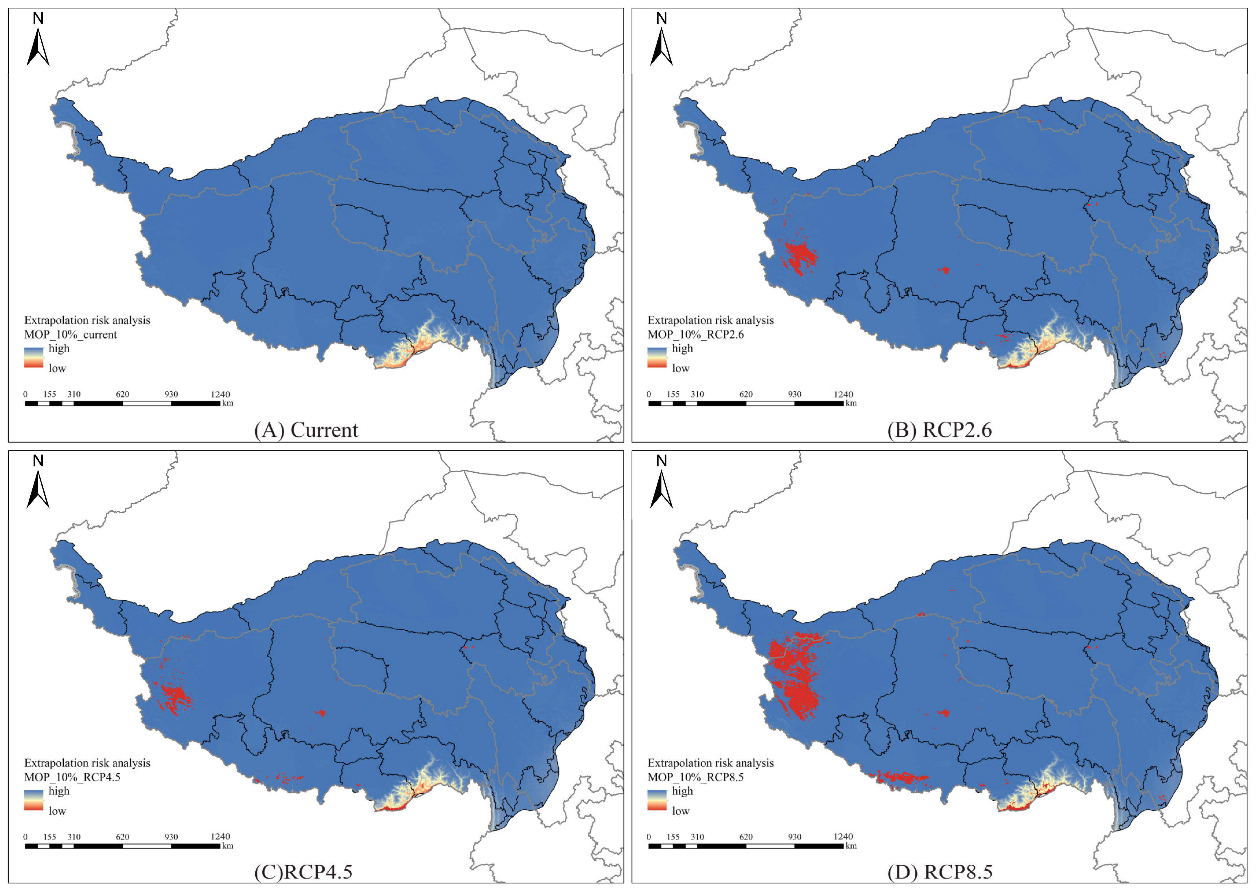
As shown in Figure 11, in the current period, the extrapolated risk index is low in the southern part of the Tibetan Plateau: Shannan and Linzhi cities, which are less suitable for the growth of Elsholtzia densa, and suitable for the growth of Elsholtzia densa in the rest of the Tibetan Plateau; in the future climate scenarios, the western and southern part of the Tibetan Plateau: Ali, Hotan, Nagqu, Shannan, Linzhi, and Shigatse, areas with an extrapolated risk index of 0 appear, and the non-suitable growth areas become larger and larger with the intensification of the greenhouse gas emission scenarios (from RCP2.6 to RCP8.5); the non-suitable growing areas become larger.

3.7. Range of Differences in Model Replications Under Different Extrapolation Methods

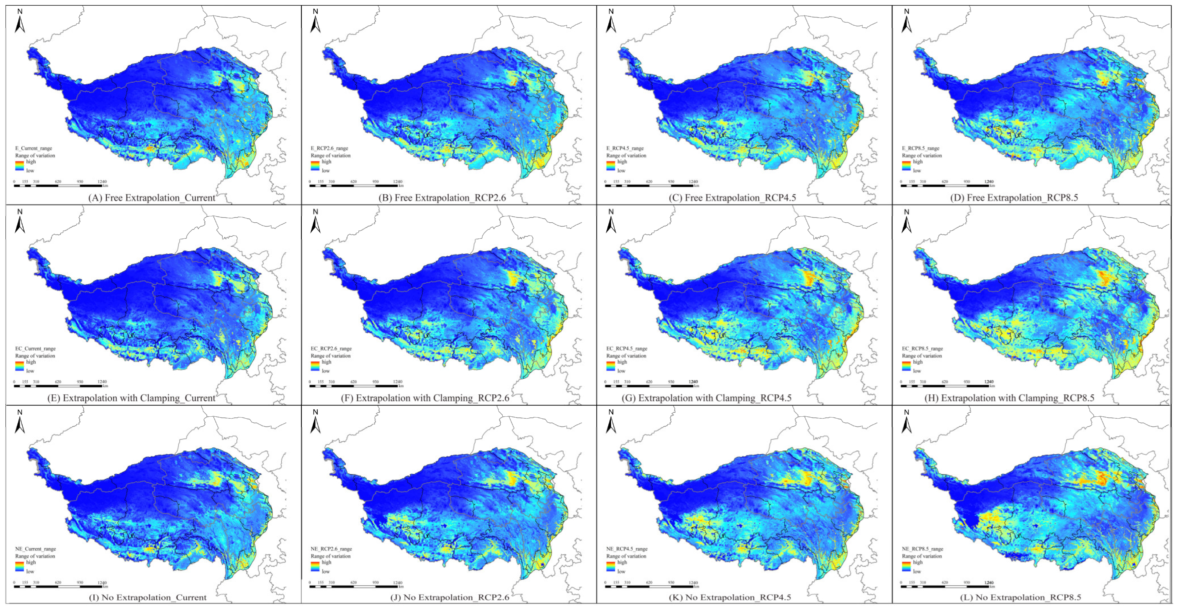
The results of this study indicate the range of variation under 10 repetitions of the model, as shown in Figure 12, with the blue area indicating a smaller range of variation over 10 repetitions, while the red area indicates a large range of variation over 10 repetitions. We find that the different extrapolation methods do not have a significant effect on the range of variation in the model repetitions, but the red area gradually increases with the intensification of the future climate scenarios. In the northwestern direction of the Tibetan Plateau, Bayinguoleng Mongol Autonomous Prefecture, Hotan City, Golmud City, Ali Region, the northern part of Nagchu City, and the western part of the Yushu Tibetan Autonomous Prefecture, the variance changes in these areas are small, and the repeatability and reliability are better; whereas in most areas in the southern and eastern parts of the Tibetan Plateau, e.g., in Yunnan, Sichuan, Gansu, the southern part of the Tibetan Autonomous Prefecture, and the eastern part of Qinghai, the 10 repetitions of the variations were larger, with lower repeatability and reliability.

3.8. MaxEnt Model Accuracy Test

Figure 13 shows the effect of the three extrapolation methods on the variance value of the 10 repetitions of the results; the three extrapolation methods do not have a significant effect on this result, and the main regions with large changes in the variance value of the 10 repetitions were Yunnan Province, the southern part of the Tibet Autonomous Prefecture, and the Haixi Tibetan-Mongolian Autonomous Prefecture, which show low reliability in multiple repetitions, while the other regions are more accurate. Especially in the northwest of the Tibetan Plateau, this result is similar to the variance range of model repetitions under different extrapolation methods, particularly in the northwestern Tibetan Plateau where the results are consistent and more accurate.
As shown in Figure 14, the variation in variance values is shown across different model parameters with regularization multipliers (RMs) of 2.5, 3.1, and 2.7. Under the E mode, the differences are concentrated in the areas of the southern part of the Tibet Autonomous Prefecture (TAP) and the northeastern part of Qinghai Province; while under the EC mode, there are some differences in the areas of the southern part of the TAP and the Yunnan Province; and under the NE mode, the differences are essentially unaffected by the between the three groups of feature combinations.
As shown in Figure 15, the variance values of different emission modes (RCP2.6, RCP4.5, RCP8.5) under the three extrapolation modes the results are extremely similar under the E and EC modes, with larger variance values in the Sichuan and Gansu provinces, the southern part of the Tibetan Autonomous Prefecture, and the eastern part of Qinghai Province. This indicates that different emission scenarios have a greater influence on the distribution of Elsholtzia densa in these regions. By contrast, the northwestern part of the Tibetan Plateau remains largely unaffected by the emission scenarios. The NE mode, however, exhibits an entirely different pattern from the E and EC modes showing minimal influence from the different emission modes, except for certain areas in Shigatse City, Shannan City, and Liangshan Yi Autonomous Prefecture.

4. Discussion

4.1. Species Distribution Modeling and Assessment of Model Effectiveness

Our study demonstrates that while multiparameter optimization significantly improves the performance of MaxEnt models, the choice of extrapolation method introduces a critical layer of uncertainty into projections of species’ range shifts under climate change. The fact that the three extrapolation approaches (E, EC, NE) yielded divergent yet plausible future distributions for Elsholtzia densa underscores the profound influence of methodological choices on model outcomes. These choices are not merely technical but reflect deeper conceptual assumptions about species’ ecological niches. The broader habitat expansion projected under the No Extrapolation (NE) approach suggests that a strictly interpolative model, when trained on current data, interprets future warming primarily as a linear shift of existing suitable conditions. In contrast, the more constrained expansion under Free Extrapolation (E) indicates that its unrestricted algorithm may anticipate nonlinear physiological limits or novel biotic interactions in new environments. The intermediate results from Extrapolation with Clamping (EC) represent a pragmatic compromise, attempting to model novelty while mechanically limiting extreme predictions. Therefore, the “most accurate” method may not exist in absolute terms but depends on the research question and one’s belief in niche conservatism versus evolvability.
The MaxEnt model was optimized using the Kuenm package [31]. Our finding was that the model combining the LQTH feature set with a regularization multiplier of 2.5 under the environmental variable set Set2 was selected as optimal. Among the 3720 candidate models, this model demonstrated the highest predictive capability. The model showed significantly lower AICc values than the alternatives, demonstrating an optimal equilibrium between complexity and precision and effectively mitigating overfitting risks. The refined model achieved an improved prediction accuracy and stronger ecological relevance [39]. Across 10 replicate runs, the mean AUC values surpassed 0.9 under all three extrapolation modes (E, EC, and NE), confirming robust prediction reliability.

4.2. Changes in Potential Suitable Areas over Time

After ripening, Elsholtzia densa can reach a height of more than 1.5 m, with numerous branches, abundant flowers, and lush foliage. Its high seed set rate results in a large number of seeds remaining in the soil, which have the characteristics of early germination, high density, and rapid growth. Certain organs of the Elsholtzia densa have allelopathic effects and tend to form dominant populations. As it continues to expand, the volatile allelopathic substances produced by its flowers and leaves inhibit the growth of other plants’ root systems and even entire plants [40]. As one of the most harmful weeds in the farmlands of the Qinghai–Tibet Plateau, Elsholtzia densa reproduces strongly and spreads rapidly, giving it a competitive advantage in population dispersion and settlement. Not only has it caused great harm to the quality and yield of rapeseed, but it has also led to changes in the plant species composition of the alpine meadows of the Qinghai–Tibet Plateau [41]. Elsholtzia densa is currently widely distributed in northwestern and southwestern China, which is consistent with the results of this study.
Research shows that under the current climatic conditions, the suitable habitat of Elsholtzia densa is predominantly distributed in the eastern and southern regions of the Tibetan Plateau, primarily encompassing the Qinghai, Sichuan, Tibet, and Gansu provinces. However, future climate warming will markedly alter habitat patterns. With increasing annual average temperatures, the expansion of suitable habitats for Elsholtzia densa increases, showing an upward trend in total suitable area. In particular, under the high-emission scenarios (RCP8.5), the outward expansion trend became the most pronounced. Different extrapolation methods affect the predicted suitable habitats of Elsholtzia densa on the Tibetan Plateau. Under the current climate, the ordering of habitat areas is E > EC > NE, whereas, in the future scenarios, the order reverses to NE > EC > E. This reversal occurs because the NE method strictly limits model extrapolation, relying more on the linear extension of historical climate data, and making it more sensitive to greenhouse-driven nonlinear warming responses. The E method allows Free Extrapolation, partially offsetting the negative impacts of extreme climatic events. Shen Yuan [42] demonstrates that future agricultural weed richness on the Tibetan Plateau will generally increase from southeast to northwest, aligning with the migration direction of Elsholtzia densa. This consistency verifies the reliability of the MaxEnt model predictions. Under future climate change conditions, rising temperatures are expected to significantly influence weed distribution [43]. Increased temperatures alter the hydrothermal conditions on the plateau, pushing weed distribution boundaries northward to higher altitudes. Consequently, crops in newly suitable areas will encounter unprecedented pressures from weeds [44].
Elsholtzia densa poses a significant threat to agroecosystems on the Qinghai–Tibet Plateau due to its vigorous reproductive capacity and allelopathic competitive advantage. Projected climate warming is anticipated to substantially expand its climatically suitable habitat, particularly towards higher altitudes and latitudes under high-emission scenarios (RCP8.5), thereby exacerbating novel threats to both cultivated crops and meadow communities.

4.3. Model Extrapolation Risks and Uncertainties

Model extrapolation refers to predictive applications outside the training data domain. For MaxEnt ecological niche models, extrapolation typically involves applying the model to environmental conditions or geographic areas not covered by the training data. This approach is particularly relevant in climate change studies where the goal is to predict the potential distributions of species under future environmental conditions. Arango-Lozano Julián [21] utilized model extrapolation risk analysis, and the MOP results indicated that turtles exhibit high similarity in occurrence areas across regions such as Caldas, Cundinamarca, Quindío, and Valle del Cauca. However, the similarity of extrapolation areas in the western region of Antioquia is relatively low. As with this study, this provides a reference for environmental similarity in niche model predictions.
Extrapolation serves as the ultimate test for the completeness of a model’s ecological mechanisms, particularly in species distribution modeling. By incorporating mechanisms such as physiological tolerance and population dynamics, the predictive reliability of models in unfamiliar environments improves [21]. This is crucial in ecological niche modeling, where extrapolation allows predictions in unobserved regions or under future climate scenarios, providing insight into species–environment relationships and distribution changes. However, as our study of Elsholtzia densa on the Qinghai–Tibet Plateau demonstrates, extrapolated predictions come with inherent uncertainty. For example, under extreme environmental conditions, such as those projected by high greenhouse gas emission scenarios (RCP8.5), extrapolation methods showed significant variation in predicting the species’ future suitable areas. Free Extrapolation (E) projected the largest suitable area, while the No Extrapolation (NE) method predicted the smallest, suggesting that Free Extrapolation could overestimate the species’ potential distribution in extreme conditions. The use of Extrapolation with Clamping (EC) helped mitigate some of this uncertainty by constraining predictions in regions with environmental extremes, offering a more balanced prediction. Our results underscore the importance of choosing appropriate extrapolation strategies, as different methods (E, EC, and NE) influenced the projected expansion of Elsholtzia densa’s suitable habitats under future climate scenarios, with implications for conservation and management decisions on the Qinghai–Tibet Plateau.

5. Conclusions

This study systematically evaluated the impacts of three extrapolation methods (Free Extrapolation, Extrapolation with Clamping, and No Extrapolation) on the prediction of suitable habitats for Elsholtzia densa on the Tibetan Plateau under current and future climate scenarios. The key findings are summarized as follows: (1) Model Optimization and Performance: Through multiparameter optimization, the model configuration with feature combination LQTH and regularization multiplier 2.5 achieved high predictive accuracy (AUC > 0.9), demonstrating the effectiveness of the Kuemn package in enhancing model robustness and mitigating overfitting. (2) Environmental Drivers: The distribution of Elsholtzia densa is primarily influenced by four bioclimatic variables: annual mean temperature (bio1), annual precipitation (bio12), mean diurnal range (bio2), and temperature annual range (bio7). Extrapolation methods had negligible effects on variable selection, underscoring the stability of these ecological determinants. (3) Spatiotemporal Dynamics: Current high-suitability areas are concentrated in the eastern and southern Tibetan Plateau. Future climate warming, particularly under high-emission scenarios (RCP8.5), is projected to significantly expand suitable habitats, with the most pronounced increases predicted under the No Extrapolation method. (4) Extrapolation Risk and Uncertainty: MESS and MoD analyses identified western and southern Tibet as regions with high climate anomaly risks, independent of extrapolation methods. Model extrapolation risk assessment further highlighted these areas as vulnerable to future unsuitability under continued warming. (5) Model Consistency: Variance analysis revealed that extrapolation methods did not significantly affect the consistency of model replicates but were sensitive to parameter settings and emission scenarios. The No Extrapolation method exhibited the least variance, suggesting higher stability in conservative projections.
This research provides a refined methodological framework for species distribution modeling through parameter optimization and systematic extrapolation analysis. It offers critical insights into the climate-driven range shifts of a pernicious agricultural weed, supporting the development of early-warning systems and targeted management strategies on the Tibetan Plateau. The findings emphasize the importance of selecting appropriate extrapolation methods in SDMs to balance predictive scope and ecological realism, thereby enhancing the reliability of climate change impact assessments on agroecosystems.

Author Contributions

Z.L.: Conceptualization, Data curation, Writing—original draft; Y.W.: Supervision, Funding acquisition, Writing—review and editing; L.C.: Methodology, Formal analysis; H.C.: Investigation, Resources; H.W.: Validation, Visualization. All authors have read and agreed to the published version of the manuscript.

Funding

This work was supported by the Qinghai Provincial Department of Science and Technology Central Government Guiding Fund for Local Science and Technology Development (2025ZY030); the Ministry of Agriculture and Rural Affairs Oat and Buckwheat Industrial Technology System Project (CARS-07-C-3); and the Supported by the Second Tibetan Plateau Scientific Expedition and Research Program (STEP) (2019QZKK0303).

Institutional Review Board Statement

Not applicable.

Informed Consent Statement

Not applicable.

Data Availability Statement

The data presented in this study are available on request from the corresponding author.

Acknowledgments

We thank colleagues at Qinghai University for field survey assistance and anonymous reviewers for constructive feedback. Special gratitude is extended to the National Meteorological Science Data Center for sharing climate datasets.

Conflicts of Interest

The authors declare that this research was conducted in the absence of any commercial or financial relationships that could be construed as a potential conflict of interest.

References

  1. Li, X.; Tian, H.; Wang, Y.; Li, R.; Song, Z.; Zhang, F.; Xu, M.; Li, D. Vulnerability of 208 endemic or endangered species in China to the effects of climate change. Reg. Environ. Change 2013, 4, 843–852. [Google Scholar] [CrossRef]
  2. IPCC. Climate Change 2007: The Physical Science Basis. Contribution of Working Group I to the Fourth Assessment Report of the Intergovernmental Panel on Climate Change; Cambridge University Press: Cambridge, UK, 2007. [Google Scholar]
  3. IPCC. Climate Change 2013: The Physical Science Basis. Contribution of Working Group I to the Fifth Assessment Report of the Intergovernmental Panel on Climate Change; Cambridge University Press: New York, NY, USA, 2013. [Google Scholar]
  4. Bellard, C.; Bertelsmeier, C.; Leadley, P.; Thuiller, W.; Courchamp, F. Impacts of climate change on the future of biodiversity. Ecol. Lett. 2012, 4, 365–377. [Google Scholar] [CrossRef]
  5. Zhao, Q.; Zhang, Y.; Li, W.-N.; Hu, B.-W.; Zou, J.-B.; Wang, S.-Q.; Niu, J.-F.; Wang, Z.-Z. Predicting the potential distribution of perennial plant Coptis chinensis Franch. in China under multiple climate change scenarios. Forest 2021, 11, 1464. [Google Scholar] [CrossRef]
  6. Liu, J.; Xin, Z.; Huang, Y.; Yu, J. Climate suitability assessment on the Qinghai-Tibet Plateau. Sci. Total Environ. 2022, 816, 151653. [Google Scholar] [CrossRef]
  7. Ji, F.; Fan, L.; Kuang, X.; Li, X.; Cao, B.; Cheng, G.; Yao, Y.; Zheng, C. How does soil water content influence permafrost evolution on the Qinghai-Tibet Plateau under climate warming? Environ. Res. Lett. 2022, 6, 064012. [Google Scholar] [CrossRef]
  8. Araújo, M.B.; Anderson, R.P.; Márcia Barbosa, A.; Beale, C.M.; Dormann, C.F.; Early, R.; Garcia, R.A.; Guisan, A.; Maiorano, L.; Naimi, B.; et al. Standards for distribution models in biodiversity assessments. Sci. Adv. 2019, 1, eaat4858. [Google Scholar] [CrossRef] [PubMed]
  9. McCune, J.L.; Baraloto, C. Species distribution models predict rare species occurrences despite significant effects of landscape context. J. Appl. Ecol. 2016, 6, 1871–1879. [Google Scholar] [CrossRef]
  10. Wang, M.; Peng, H.; Bai, Y.; Bai, Q.; Zhang, Q.; Feng, Y.; Wang, J.; Tang, Y. Impacts of physiological characteristics and human activities on the species distribution models of orchids taking the Hengduan Mountains as a case. Ecol. Evol. 2023, 13, e10566. [Google Scholar] [CrossRef] [PubMed]
  11. Tang, Y.; Winkler, A.; Viña, A.; Liu, J.; Zhang, Y.; Zhang, X.; Li, X.; Wang, F.; Zhang, J.; Zhao, Z. Uncertainty of future projections of species distributions in mountainous regions. PLoS ONE 2018, 13, e0189496. [Google Scholar] [CrossRef] [PubMed]
  12. Elith, J.; Phillips, S.J.; Hastie, T.; Dudík, M.; Chee, Y.E.; Yates, C.J. A statistical explanation of MaxEnt for ecologists. Divers. Distrib. 2011, 1, 43–57. [Google Scholar] [CrossRef]
  13. Elith, J.; Graham, H.C.; Anderson, R.P.; Dudík, M.; Ferrier, S.; Guisan, A.; Hijmans, R.J.; Huettmann, F.; Leathwick, J.R.; Lehmann, A.; et al. Novel methods improve prediction of species’ distributions from occurrence data. Ecography 2006, 2, 129–151. [Google Scholar] [CrossRef]
  14. Jiang, C.; Zhang, X.; Xie, W.; Wang, R.; Feng, C.; Ma, L.; Li, Q.; Yang, Q.; Wang, H. Predicting the potential distribution of the fall armyworm Spodoptera frugiperda (J.E. Smith) under climate change in China. Glob. Ecol. Conserv. 2022, 33, e01994. [Google Scholar] [CrossRef]
  15. Phillips, S.J.; Anderson, R.P.; Schapire, R.E. Maximum entropy modeling of species geographic distributions. Ecol. Model. 2006, 190, 231–259. [Google Scholar] [CrossRef]
  16. Zhong, Y.; Xue, Z.; Jiang, M.; Liu, B.; Wang, G. The application of species distribution modeling in wetland restoration: A case study in the Songnen Plain, Northeast China. Ecol. Indic. 2021, 121, 107137. [Google Scholar] [CrossRef]
  17. Cobos, M.E.; Peterson, A.T.; Barve, N.; Osorio-Olvera, L. kuenm: An R package for detailed development of ecological niche models using Maxent. PeerJ 2019, 7, e6281. [Google Scholar] [CrossRef] [PubMed]
  18. Shen, S.; Zheng, F.; Zhang, W.; Xu, G.; Li, D.; Yang, S.; Jin, G.; Clements, D.R.; Nikkel, E.; Chen, A.; et al. Potential distribution and ecological impacts of Acmella radicans (Jacquin) R.K. Jansen (a new Yunnan invasive species record) in China. BMC Plant Biol. 2024, 24, 494. [Google Scholar] [CrossRef]
  19. Jiao, X.; Long, M.; Li, J.; Yang, Q.; Liu, Z. Reconstructing the Invasive History and Potential Distribution Prediction of Amaranthus palmeri in China. Agronomy 2023, 13, 2498. [Google Scholar] [CrossRef]
  20. Scherrer, D.; Esperon-Rodriguez, M.; Beaumont, L.J.; Barradas, V.L.; Guisan, A. National assessments of species vulnerability to climate change strongly depend on selected data sources. Divers. Distrib. 2021, 8, 1367–1382. [Google Scholar] [CrossRef]
  21. Arango Lozano, J.; Patiño Siro, D.; Toro Cardona, F. Reaching new environments through illegal trade: Evidence of a widely traded turtle in Colombia. Aquat. Ecol. 2023, 2, 471–480. [Google Scholar] [CrossRef]
  22. Yang, J.; Du, J.; Yu, F.; Li, R.; Zhong, J. Two new compounds from the aerial parts of Elsholtzia densa. Phytochem. Lett. 2022, 52, 104–108. [Google Scholar] [CrossRef]
  23. Editorial Committee of Flora of China, Chinese Academy of Sciences. Flora Reipublicae Popularis Sinicae; Science Press: Beijing, China, 1977; p. 332. (In Chinese) [Google Scholar]
  24. Li, Z.; Ji, Q.; Yang, Y.; Gao, Y.; Xu, M.; Guan, Y. Predicting suitable habitats for Elsholtzia densa on the Qinghai-Xizang (Tibetan) Plateau under climate change using the Biomod2 model. Agric. Res. Arid Areas 2025, 3, 278–286. (In Chinese) [Google Scholar] [CrossRef]
  25. Zhou, X.; Xiao, Y.; Ma, D.; Xie, Y.; Wang, Y.; Zhang, H.; Wang, Y. The competitive strategies of poisonous weeds Elsholtzia densa Benth. on the Qinghai Tibet Plateau: Allelopathy and improving soil environment. Front. Plant Sci. 2023, 14, 1124139. [Google Scholar] [CrossRef]
  26. GBIF Occurrence Download. Available online: https://doi.org/10.15468/dl.b8sx2a (accessed on 14 April 2024).
  27. Warren, D.L.; Matzke, N.J.; Cardillo, M.; Baumgartner, J.B.; Beaumont, L.J.; Turelli, M.; Glor, R.E.; Huron, N.A.; Simões, M.; Iglesias, T.L.; et al. ENMTools 1.0: An R package for comparative ecological biogeography. Ecography 2021, 44, 504–511. [Google Scholar] [CrossRef]
  28. NGIC. Administrative Boundaries Data at 1:1,000,000 Scale Over the Tibetan Plateau 2017. National Tibetan Plateau/Third Pole Environment Data Center. 2019. Available online: https://cstr.cn/18406.11.Geogra.tpdc.270001 (accessed on 23 June 2024).
  29. Jiang, R.; Zou, M.; Qin, Y.; Tan, G.; Huang, S.; Quan, H.; Zhou, J.; Liao, H. Modeling of the Potential Geographical Distribution of Three Fritillaria Species Under Climate Change. Front. Plant Sci. 2022, 12, 749838. [Google Scholar] [CrossRef]
  30. Zhu, G.; Bu, W.; Gao, Y.; Liu, G. Potential geographic distribution of brown marmorated stink bug invasion (Halyomorpha halys). PLoS ONE 2012, 2, e31246. [Google Scholar] [CrossRef]
  31. Chen, S.; Bai, X.; Ye, J.; Chen, W.; Xu, G. Prediction of Suitable Habitat of Alien Invasive Plant Ambrosia trifida in Northeast China under Various Climatic Scenarios. Diversity 2024, 16, 322. [Google Scholar] [CrossRef]
  32. Zhang, B.; Xie, Z.; Ma, Y.; Zhao, Y.; Wei, C.; Fu, Y.; Liu, M.; Xu, F. Analysis on Changes in Suitable Areas for Fagopyrum dibotrys under Climate Change Scenarios in China. Chin. J. Agrometeorol. 2024, 8, 835–848. [Google Scholar] [CrossRef]
  33. Morales, N.S.; Fernandez, I.C.; Baca-Gonzalez, V. MaxEnt’s parameter configuration and small samples: Are we paying attention to recommendations? A systematic review(Article). PeerJ 2017, 3, e3093. [Google Scholar] [CrossRef] [PubMed]
  34. Hanley, J.A.; McNeil, B.J. The meaning and use of the area under a receiver operating characteristic (ROC) curve. Radiology 1982, 1, 29–36. [Google Scholar] [CrossRef]
  35. Zhuo, Z.; Xu, D.; Pu, B.; Wang, R.; Ye, M. Predicting distribution of Zanthoxylum bungeanum Maxim. in China. BMC Ecol. 2020, 20, 46. [Google Scholar] [CrossRef] [PubMed]
  36. Motloung, R.F.; Chaisi, M.E.; Sibiya, M.S.; Nyangiwe, N.; Shivambu, T.C. Predicting tick distributions in a changing climate: An ensemble approach for South Africa. Vet. Parasitol. 2025, 338, 110528. [Google Scholar] [CrossRef]
  37. Elith, J.; Kearney, M.; Phillips, S. The art of modelling range-shifting species. Methods Ecol. Evol. 2010, 4, 330–342. [Google Scholar] [CrossRef]
  38. Owens, H.L.; Campbell, L.P.; Dornak, L.L.; Saupe, E.E.; Barve, N.; Soberón, J.; Ingenloff, K.; Lira-Noriega, A.; Hensz, C.M.; Myers, C.E.; et al. Constraints on interpretation of ecological niche models by limited environmental ranges on calibration areas. Ecol. Model. 2013, 263, 10–18. [Google Scholar] [CrossRef]
  39. Quiroga, M.P.; Souto, C.P. Ecological niche modeling, niche overlap, and good old Rabinowitz’s rarities applied to the conservation of gymnosperms in a global biodiversity hotspot. Landsc. Ecol. 2022, 10, 2571–2588. [Google Scholar] [CrossRef]
  40. He, S.; Gu, C.; Ma, D.; Zhang, H. Regulation of ROS and NO in Chenopodium ambrosioides allelopathic stress-induced death of Vicia faba root border cells. Acta Ecol. Sin. 2022, 2, 818–827. (In Chinese) [Google Scholar] [CrossRef]
  41. Song, Z.; Li, X.; Li, J.; Ka, Z.; Ma, G. Effects of plateau pika (Ochotona curzoniae) trails on enlargement and connection of degraded patches in alpine meadow. Chin. J. Ecol. 2020, 10, 3276–3284. (In Chinese) [Google Scholar] [CrossRef]
  42. Shen, Y.; Qiu, P.; Liao, Z.Y.; Wu, X.G.; Sun, X.M.; Zhang, L.; Pan, Z.F.; Pan, K.W. Changes in distribution patterns of weed species richness in agricultural lands on Qinghai-Tibet Plateau under climate change. Chin. J. Appl. Environ. Biol. 2022, 4, 897–908. (In Chinese) [Google Scholar] [CrossRef]
  43. Wang, C.J.; Wan, J.Z. Assessing the habitat suitability of 10 serious weed species in global croplands. Glob. Ecol. Conserv. 2020, 3, 142–153. [Google Scholar] [CrossRef]
  44. Root, T.L.; Price, J.T.; Hall, K.R.; Schneider, S.H.; Rosenzweig, C.; Pounds, J.A. Fingerprints of global warming on wild animals and plants. Nature 2003, 421, 57–60. [Google Scholar] [CrossRef] [PubMed]
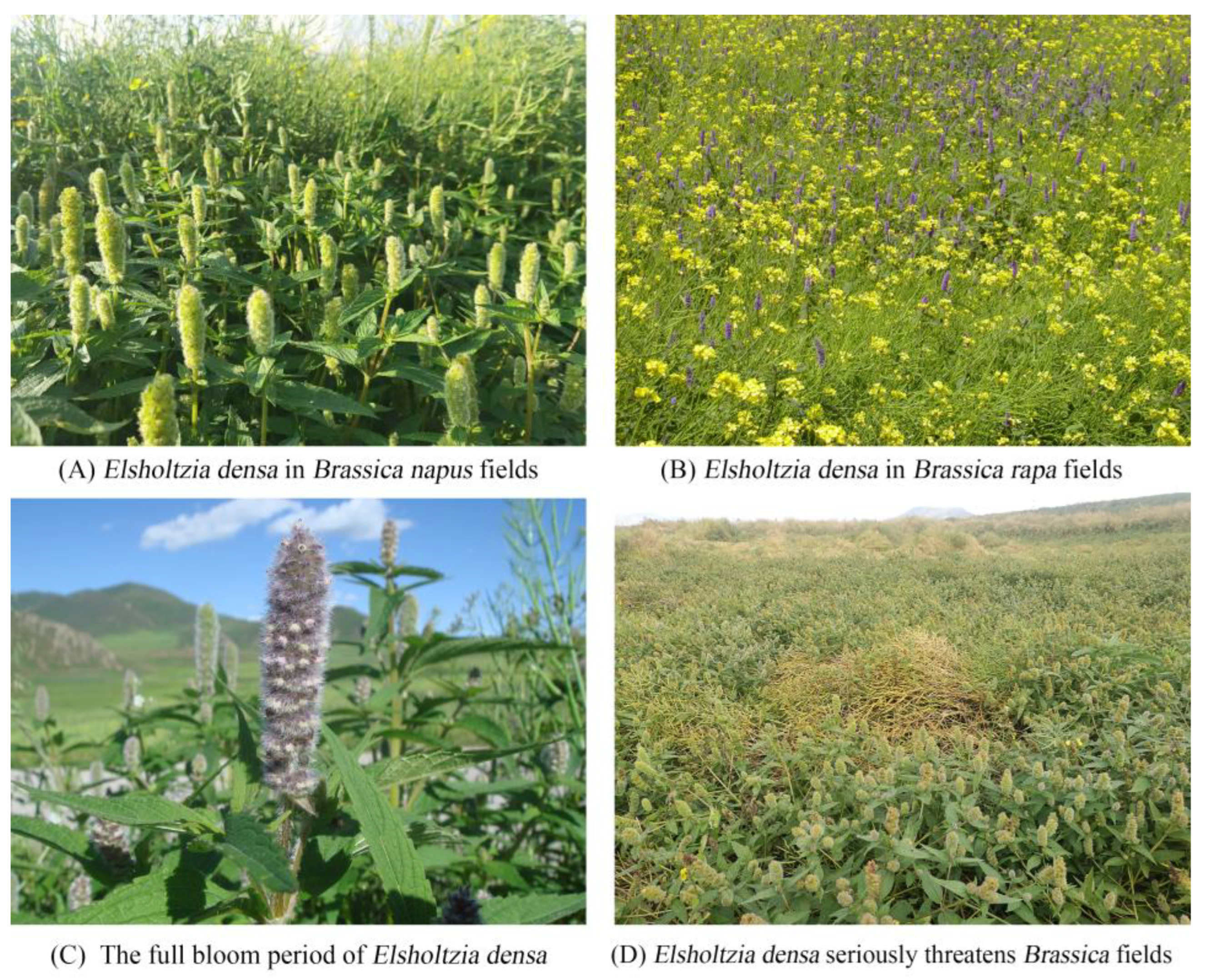
Figure 1. Field investigation of Elsholtzia densa.
Sustainability 17 08206 g001
Figure 2. Distribution of Elsholtzia densa on the Qinghai–Tibet Plateau. This figure was created using a map of the Qinghai–Tibet Plateau downloaded from the National Qinghai–Tibet Plateau Science Data Center website (https://data.tpdc.ac.cn/home, accessed on 23 June 2024) [28]. The base map has not been modified. The same applies to the following figures.
Sustainability 17 08206 g002
Figure 3. The model selection results in R program.
Sustainability 17 08206 g003
Figure 4. The response curves of key environmental variables under the Free Extrapolation method. X-axis: range of the climatic factor; Y-axis: probability of occurrence. Hereafter, these are the same.
Sustainability 17 08206 g004
Figure 5. The response curves of key environmental variables under the Extrapolation with Clamping method.
Sustainability 17 08206 g005
Figure 6. The response curves of key environmental variables under the No Extrapolation method.
Sustainability 17 08206 g006
Figure 7. MaxEnt model predicted potential habitat areas of Elsholtzia densa at different times under different extrapolation methods. (AD) are Free Extrapolations; (EH) are Extrapolations with Clamping; (IL) are No Extrapolation; all are divided into four suitable areas according to a unified standard: potential low suitable region, potential moderately suitable region, and potential high suitable region.
Sustainability 17 08206 g007
Figure 8. Changes in spatial pattern of the suitable area of Elsholtzia densa at different times under different extrapolation methods. The shaded or tonally accentuated region delineates the spatial extent of the Tibetan Plateau, whereas the contour lines beyond this zone represent the national boundaries of China. This convention of representation is consistently maintained in all subsequent figures.
Sustainability 17 08206 g008
Figure 9. Multivariate environmental similarity surface predicted by the MaxEnt model for the next three periods under different extrapolation methods.
Sustainability 17 08206 g009
Figure 10. The most dissimilar variable predicted by the MaxEnt model for the next three periods under different extrapolations.
Sustainability 17 08206 g010
Figure 11. Model extrapolated risk for different time periods. The red areas indicate an extrapolation risk index of 0, the blue areas indicate a high extrapolation risk index, and the other colored areas are in between.
Sustainability 17 08206 g011
Figure 12. Comparison of the range of differences between the 10 replications of the model in each period for different extrapolation methods. (AD) are Free Extrapolation; (EH) are Extrapolation with Clamping; (IL) are No Extrapolation. The color gradient from red to blue represents the spectrum of variation across the 10 replicates, with red hues indicating regions of higher variability among the repetitions, while blue hues denote areas of lower variability.
Sustainability 17 08206 g012
Figure 13. Variation in variance of model results from 10 repetitions under three extrapolation methods. (A) is Free Extrapolation; (B) is Extrapolation with Clamping; (C) is No Extrapolation. The brighter the color in the figure, the greater the variance value.
Sustainability 17 08206 g013
Figure 14. Variation in variance of model results from different parameters under three extrapolation methods. (A) is Free Extrapolation; (B) is Extrapolation with Clamping; (C) is No Extrapolation. The brighter the color in the figure, the greater the variance value.
Sustainability 17 08206 g014
Figure 15. Changes in variance values for different emission scenarios under three extrapolation methods. (A) is Free Extrapolation; (B) is Extrapolation with Clamping; (C) is No Extrapolation. The brighter the color in the figure, the greater the variance value.
Sustainability 17 08206 g015
Table 1. Field investigation distribution points of Elsholtzia densa.
LocationAltitude (m)East
Longitude
North
Latitude
Zhongchuan Township, Minhe County1790102°51′36.81″35°52′12.09″
Jishi Town, Xunhua County1871102°28′50.64″35°51′02.92″
Gaomiao Town, Ledu County1936102°32′29.58″36°26′36.41″
Donggou Township, Minhe County2208102°42′58.71″36°09′29.52″
Gushan Township, Minhe County2219102°48′31.61″36°05′41.03″
Hexi Township, Guide County2227101°23′13.12″36°02′03.90″
Manping Township, Minhe County2286102°46′35.74″36°01′28.35″
Shatangchuan Township, Huzhu County2332101°53′49.92″36°41′46.27″
Sanhe Township, Ping ‘an County2391101°56′56.67″36°25′39.10″
Zongzhai Township, Huangzhong County2422101°41′19.08″36°32′57.64″
Shuangshu Township, Huzhu County2425101°55′00.47″36°46′26.25″
Lijiashan Township, Ledu County2436102°44′28.95″36°07′21.44″
Shagou Township, Ping ‘an County2508102°02′43.71″36°23′44.27″
Wufeng Township, Huzhu County2530101°51′21.42″36°52′36.72″
Tianjiazhai Township, Huangzhong County2584101°48′53.74″36°24′53.71″
Machang Township, Ledu County2585102°45′22.38″36°26′37.17″
Gangou Township, Minhe County2585102°46′30.54″37°24′14.95″
Tumen Pass Township, Huangzhong County2597101°43′41.09″36°26′28.93″
Dacai Township, Huangzhong County2610101°28′56.18″36°30′52.13″
Lime Kiln Township, Ping ‘an County2619101°53′37.16″36°22′52.00″
Shizhang Township, Huangzhong County2644101°45′25.68″36°24′08.99″
Hualin Township, Datong County2646101°43′57.96″37°02′02.65″
Luhua Township, Ledu County2653102°43′11.30″36°32′55.21″
Angsi Duo, Hualong County2655102°03′50.57″36°10′15.45″
Taizi Township, Huzhu County2661101°56′15.04″36°54′58.54″
Chengguan Township, Huangyuan County2671101°15′56.50″36°41′19.23″
Duolin Township, Datong County2672101°27′39.63″37°03′43.58″
Zaba Township, Hualong County2702101°59′41.22″36°12′23.76″
Baoku Township, Datong County2705101°34′10.56″37°06′53.28″
Dahua Township, Huangyuan County2705101°12′00.91″36°42′55.99″
Heping Township, Huangyuan County2709101°15′25.85″36°37′26.70″
Shidacang Township, Hualong County2725102°21′17.03″36°05′55.13″
Tangnaihai Township, Xinghai County2729100°08′30.88″35°30′39.82″
Zama Shi Township, Qilian County2741100°03′40.17″38°12′59.43″
Xiejiatan Township, Hualong County2749102°16′32.00″36°04′55.03″
Chuankou Town, Menyuan County2751101°51′14.50″37°19′11.10″
Babao Township, Qilian County2754100°15′00.68″38°10′23.07″
Bohang Township, Huangyuan County2765101°12′33.87″36°39′48.37″
Qushi ‘an Township, Xinghai County2767100°14′01.28″35°19′31.49″
Maying Township, Ledu County2768102°39′34.88″36°33′14.39″
Gucheng Town, Ping ‘an County2789101°59′25.11″36°19′13.97″
Nuomuhong Township, Dulan County279196°27′26.91″36°26′07.85″
Bayan Township, Huangyuan County2806101°08′03.19″36°46′00.25″
Hedong Township, Golmud City281094°54′43.96″36°24′53.97″
Qingshan Township, Datong County2815101°23′46.29″37°05′29.93″
Dayuan Township, Huangzhong County2824101°31′18.56″36°27′51.40″
Chabuqia Town, Gonghe County2840100°36′55.75″36°16′40.85″
Bayan Township, Hualong County2841102°14′58.05″36°06′58.00″
Huaitoutala Township, Delingha City287296°44′51.06″37°21′01.87″
Shazhuyu Township, Gonghe County2877100°15′42.99″36°15′39.80″
Hongshuiquan Township, Ping ‘an County2879101°53′25.42″36°27′45.39″
Nanmenxia Township, Huzhu County2880101°54′27.02″37°00′17.55″
Donghe Township, Huzhu County2887102°03′39.37″36°55′13.51″
Bagou Township, Tongde County2890100°20′11.30″35°17′46.66″
Qingshizui Town, Menyuan County2970101°23′38.84″37°28′29.15″
Gannan Village, Delingha City297797°22′13.52″37°21′21.66″
Ertang Township, Hualong County2979102°11′56.13″36°08′05.85″
Riyue Township, Huangyuan County3018101°09′22.72″36°31′07.00″
Wulan County Town305298°31′51.02″36°56′02.44″
Tangge Mu, Gonghe County305799°57′50.57″36°12′07.24″
Tongpu Township, Wulan County308198°32′09.14″36°59′48.01″
Xiangride Township, Dulan County308497°51′30.92″35°59′13.34″
Tiegai Township, Gonghe County3103100°12′32.47″35°59′47.78″
Guomaying Township, Guinan County3106101°06′49.74″35°48′38.11″
Mangqu Township, Guinan County3122100°46′50.88″35°34′11.97″
Laiyihai Township, Guinan County3164100°46′31.61″35°34′09.45″
Sizhai Township, Huangyuan County3172101°02′13.26″36°45′11.25″
Chasu Town, Dulan County319098°05′17.39″36°17′50.82″
Tanggu Town, Tongde County3316100°32′08.30″35°11′26.50″
Table 2. Nineteen bioclimatic variables.
Climate FactorsNameUnit
bio1Annual mean temperature°C
bio2Mean diurnal temperature range°C
bio3Isothermality-
bio4Temperature seasonality
(standard deviation × 100)
-
bio5Maximum temperature of warmest month°C
bio6Minimum temperature of coldest month°C
bio7Temperature annual range°C
bio8Mean temperature of wettest quarter°C
bio9Mean temperature of driest quarter°C
bio10Mean temperature of warmest quarter°C
bio11Mean temperature of coldest quarter°C
bio12Annual precipitationmm
bio13Precipitation of wettest monthmm
bio14Precipitation of driest monthmm
bio15Precipitation seasonalitymm
bio16Precipitation of wettest quartermm
bio17Precipitation of driest quartermm
bio18Precipitation of warmest quartermm
bio19Precipitation of coldest quartermm
Table 3. The model selection results in R program.
ModelMean_AUC_ratiopval_pROCOmission_rate_at_5%AICcdelta_AICcW_AICcnum_parameters
M_2.5_F_LQTH_Set21.66106700.0555562999.5890128
M_3.1_F_LQTH_Set21.65633100.0555563001.3451.756348124
M_2.7_F_LQTH_Set21.67147600.0555563001.4371.847758127
Table 4. Suitable ranges for key environmental factors under different extrapolation methods.
Environmental VariablesFree
Extrapolation
Extrapolation
with Clamping
No
Extrapolation
bio1 (Annual mean
temperature)
2.5–8.6 °C2.6–9.0 °C2.6–9.0 °C
bio2 (Mean diurnal
temperature range)
13.7–16.5 °C13.4–15.4 °C13.5–15.7 °C
bio7 (Temperature annual range)25.4–35.6 °C24.6–34.5 °C26.9–34.3 °C
bio12 (Annual precipitation)490.2–715.5 mm469.1–738.5 mm451.4–815.3 mm
Table 5. Changes in the size of the suitable area of Elsholtzia densa at different times under the three extrapolation methods.
Extrapolation ModelPeriodsLow
Suitability Area (×104 km2)
Trends (×104 km2)Moderate Suitability Area (×104 km2)Trends (×104 km2)High
Suitability Area (×104 km2)
Trends (×104 km2)
ECurrent32.05-16.32-7.88-
RCP2.640.35↑ 8.322.97↑ 6.6520.21↑ 12.33
RCP4.542.39↑ 10.3427.04↑ 10.7229.17↑ 21.29
RCP8.543.41↑ 11.3633.01↑ 16.6941.93↑ 34.05
ECCurrent34.39-17.48-7.73-
RCP2.643.21↑ 8.8224.82↑ 7.3419.93↑ 12.20
RCP4.545.00↑ 10.6229.60↑ 12.1329.01↑ 21.28
RCP8.545.80↑ 11.4136.26↑ 18.7840.87↑ 33.14
NECurrent33.77-17.16-8.15-
RCP2.642.42↑ 8.6425.55↑ 8.3821.13↑ 12.99
RCP4.544.52↑ 10.7531.05↑ 13.8831.11↑ 22.97
RCP8.545.41↑ 11.6435.89↑ 18.7345.21↑ 37.07
Note: ↑ represents an increase in the suitable area compared with the control group.
Table 6. Spatial changes of Elsholtzia densa habitats under climate scenarios with the three extrapolation methods.
Extrapolation ModelClimate
Scenarios
Area (×104 Km2)
Persistently UnsuitableSuitability
Gain
Suitability LossPersistently Suitable
RCP2.6146.5227.430.0781.07
ERCP4.5130.1943.760.1081.03
RCP8.5112.2561.700.0381.10
RCP2.6151.1628.040.1875.70
ECRCP4.5134.8444.370.2075.68
RCP8.5117.4861.720.1575.73
RCP2.6151.3430.110.8072.84
NERCP4.5133.3648.090.9472.69
RCP8.5114.5766.881.7171.93
Disclaimer/Publisher’s Note: The statements, opinions and data contained in all publications are solely those of the individual author(s) and contributor(s) and not of MDPI and/or the editor(s). MDPI and/or the editor(s) disclaim responsibility for any injury to people or property resulting from any ideas, methods, instructions or products referred to in the content.