Abstract
Urban air pollution remains a significant environmental and public health issue, especially in European coastal cities such as Klaipėda. However, there is still a lack of local-scale knowledge on how land use structure influences pollutant distribution, highlighting the need to address this gap. This study addresses this by examining the spatial distribution of nitrogen dioxide (NO2) concentrations in Klaipėda’s seaport city and several inland and coastal resort towns in Lithuania. The research specifically asks how different land cover types and demographic factors affect NO2 variability and population exposure risk. Data were collected using passive sampling methods and analyzed within a GIS environment. The results revealed clear air quality differences between industrial/port zones and greener resort areas, confirmed by statistically significant associations between land cover types and pollutant levels. Based on these findings, a Land Use Pollution Pressure index (LUPP) and its population-weighted variant (PLUPP) were developed to capture demographic sensitivity. These indices provide a practical decision-support tool for sustainable urban planning, enabling the assessment of pollution risks and the forecasting of air quality changes under different land use scenarios, while contributing to local climate adaptation and urban environmental governance.
1. Introduction
Urban air pollution is a significant environmental and public health issue, especially in European coastal cities such as Klaipėda. According to European Union data, air pollution reduces average life expectancy by approximately seven years. However, there is no scientific evidence of a threshold below which air pollution does not impact health [1]. In Lithuania, Klaipėda city—as the country’s major seaport—faces specific air quality challenges related to industrial and maritime activities, while inland and coastal resort towns are characterized by higher green coverage and lower NO2 levels. This contrast highlights the urgency to understand how land use patterns drive local air pollution risks. Therefore, this study raises the question of how different land cover types influence spatial NO2 variability and population exposure in contrasting urban settings. To better assess these differences, it is essential to clarify the role that specific land use types—from industrial zones to transport infrastructure and residential areas—play in amplifying or mitigating local pollution pressure.
In industrial sectors, the installation of filtering systems and advanced emission control technologies has led to measurable reductions in pollutants such as sulfur oxides (SOx), sulfur dioxide (SO2), volatile organic compounds (VOCs), and heavy metals. Recent studies confirm these trends—the implementation of modern emission control technologies in industrial operations has significantly decreased VOCs and heavy metal emissions, while sulfur compounds have also shown marked reductions due to regulatory enforcement and technical upgrades [2]. However, despite significant improvements in industrial pollution management, the transport sector—as a core component of urban land use—remains a major contributor to air pollution globally. In Lithuania, transport-related land use, particularly road networks and high-traffic corridors, accounts for nearly one-third of all air pollutant emissions, with nitrogen dioxide (NO2) and particulate matter (PM10) being the most prevalent. This pattern reflects a broader European trend: according to a Joint Research Centre report, transport infrastructure—including roads, railways, and airports—continues to dominate urban and regional NO2 levels across the EU due to fossil fuel combustion and dense traffic flows [3]. These patterns emphasize that transport infrastructure should not be treated in isolation but as an integral element of the built environment, reinforcing how land use intensity and transport networks together shape local NO2 concentrations.
Extensive research shows that green spaces embedded in dense urban land use can significantly reduce concentrations of major air pollutants, including NO2, through canopy interception and surface deposition. Forests, in particular, play a vital role in absorbing and filtering airborne pollutants, functioning as natural biofilters. Some studies discuss the physiological and molecular functions of urban forests in improving air quality and reducing pollutant loads [4]. These findings highlight that conserving and expanding urban green areas is critical to balancing the impacts of intensive land use and transport-related emissions, with direct implications for sustainable urban planning.
To better capture how these combined land use dynamics affect NO2 levels spatially, researchers increasingly rely on spatially explicit modeling tools, particularly Land Use Regression (LUR) models. These models have proven effective in assessing the spatial distribution of air pollutants across urban environments. For example, previous researchers [5] have used LUR to estimate personal exposure to traffic-related pollutants, while others [6] have employed spatial regression to evaluate the effectiveness of congestion charging schemes in London. More recent studies [7] have further expanded the utility of LUR by integrating satellite data and chemical transport models, demonstrating the method’s adaptability across different geographic and urban contexts.
Despite these methodological advances, the application of LUR-type models in Lithuania remains limited—particularly when examining how urban morphology and land use patterns shape NO2 concentrations and population exposure. This highlights a clear gap in local urban environmental assessment and evidence-based planning. To address this need, the present study proposes a context-adapted spatial assessment framework—the Land Use Pollution Pressure (LUPP) index—specifically developed for urban settings like Klaipėda. In this study, “pollution pressure” is defined as the combined structural effect of land use intensity, land cover types, and urban form that amplifies or mitigates pollutant concentrations in specific locations. This framework combines passive NO2 measurements, GIS-based land cover analysis, and a diagnostic index that quantifies structural pollution pressure in relation to land use intensity. Unlike conventional LUR models that rely on extensive regression with large datasets, the LUPP index functions as a practical, transferable tool that can support planning decisions even in data-limited contexts. It does not aim to precisely predict emissions but rather provides a diagnostic basis for understanding how urban structure and land cover configuration influence local pollution pressure.
In Klaipėda—a city where the seaport is integrated into the urban core and prevailing winds often direct emissions toward residential areas—the approach was adapted to local conditions. To strengthen the social dimension, a population-weighted version (PLUPP) was developed to reflect demographic sensitivity, giving special attention to groups more vulnerable to air pollution, such as children and the elderly.
The resulting assessment framework offers a locally adaptable method for evaluating structural pollution pressure and demographic vulnerability. While the general approach is transferable to other urban environments, its interpretation requires local calibration to reflect specific land cover and population structures. This practical perspective encourages integration of structural and social aspects of air pollution exposure into urban environmental management, rather than claiming technological novelty.
2. Materials and Methods
2.1. Study Area
The primary study area is Klaipėda (54°43′16″ N, 21°07′ E), Lithuania’s third-largest city and principal seaport, located on the southeastern Baltic Sea coast. Klaipėda’s distinctive urban structure—combining industrial, port, and residential zones within a compact area of approximately 98 km2 and a population of around 166,000—creates a complex environmental landscape. The Port of Klaipėda, located adjacent to the city center, handles significant maritime traffic, contributing notably to local air pollution.
Given Klaipėda’s coastal location and proximity to the open Baltic Sea, meteorological factors—particularly prevailing wind patterns—play a critical role in shaping the dispersion and accumulation of atmospheric pollutants within the urban environment. Prevailing winds in the Klaipėda region are primarily from the west and southwest, particularly during the cold season. These meteorological patterns are driven by large-scale circulation processes in the southeastern Baltic and are recognized as critical factors influencing the transport of atmospheric pollutants from port and industrial areas into residential zones. Such wind dynamics and long-term trends have been documented in climate research focused on the Lithuanian coastal zone [8].
While prevailing winds largely determine the direction of pollutant dispersion, the effectiveness of local air quality regulation also depends on land cover characteristics—particularly the presence of green spaces, which are known to reduce airborne pollutant concentrations through deposition and absorption processes [9]. Klaipėda’s relatively low proportion of forests and green spaces limits the city’s natural capacity to mitigate air pollutants. This urban–industrial setting presents an ideal environment for assessing how specific land use structures influence ambient concentrations of nitrogen dioxide (NO2) and particulate matter (PM). According to national air quality reports, Klaipėda consistently exhibits elevated concentrations of these pollutants, particularly in areas adjacent to the seaport and major transport corridors. This observation is further supported by previous studies, which identified port operations and heavy transport routes as the most pollution-intensive zones within the city. Specifically, elemental analyses of airborne particulates have shown that chemical elements such as tungsten (W), lead (Pb), and zinc (Zn) are most concentrated in areas affected by intense port-related activities and freight traffic [10].
Figure 1 presents the urban area of Klaipėda, highlighting all air quality monitoring stations used during the 2023 measurement campaign [11]. These stations captured ambient air pollution levels across different parts of the city and served to establish baseline conditions characteristic of Klaipėda’s urban–industrial environment.
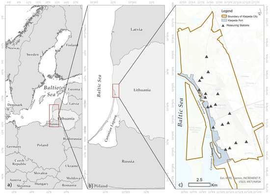
Figure 1.
The study area: southeast part (SE) of the Baltic Sea (a); Klaipeda city (b); air pollution measuring stations (MS) by urban functional area (c) 2023.
Building upon the 2023 campaign depicted in Figure 1, Figure 2 presents an expanded spatial and temporal framework introduced in 2024. This new phase of data collection extended the study beyond Klaipėda to include selected Lithuanian resort and therapeutic towns—Palanga, Birštonas, Druskininkai (two sites), and Abromiškės. This expansion aimed to investigate nitrogen dioxide (NO2) concentrations across functionally and environmentally distinct settings.
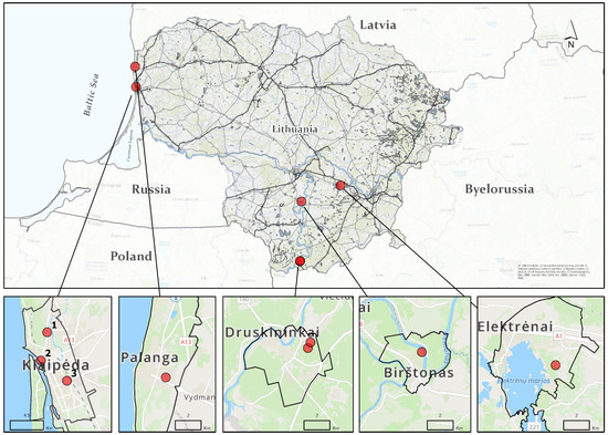
Figure 2.
NO2 monitoring sites across Lithuanian resorts and comparative urban zones in Klaipėda 2024.
In addition to these resort locations, three strategically selected sites within Klaipėda were also included in the 2024 campaign. These Klaipėda sites were chosen based on findings from the 2023 baseline study and represent contrasting urban functions: (1) the cleanest residential neighborhood, (2) the most polluted port-related area, and (3) a high-traffic transportation hub. Their inclusion enabled direct comparison with the resort towns, ensuring consistency in the interpretation of NO2 concentration patterns across varied land uses under similar seasonal and meteorological conditions.
Palanga, situated along the Baltic Sea coast, represents a coastal resort town with low industrial development and abundant natural landscapes. Birštonas and Druskininkai, located inland, are traditional spa towns characterized by extensive forests and recreational infrastructure, supporting lower levels of vehicular and industrial emissions. Abromiškės, while not a typical tourist resort, functions as a national rehabilitation hospital area featuring semi-natural land cover and minimal anthropogenic pollution sources.
The selected resort areas, characterized by high proportions of natural land cover and limited industrial activity, are known for their favorable environmental conditions and consistently lower air pollutant levels [9]. These structural and functional features provide a relevant contrast to Klaipėda’s urbanized context. This comparison enables the assessment of how environmental structure alone—independent of changes in transport intensity or population density—affects ambient air quality. By establishing both temporal continuity (through Klaipėda measurements across 2023 and 2024) and spatial contrast (between urban and resort-type areas), this study provides a robust basis for evaluating the role of land use and environmental context in shaping urban air pollution patterns.
2.2. Data and Methods
2.2.1. Air Quality Monitoring and GIS Buffer Approach
During the 2023–2024 period, a citywide air quality monitoring campaign was conducted in Klaipėda port industrial city to assess seasonal variations and spatial distribution of pollution. Nitrogen dioxide (NO2) concentrations were measured using passive diffusive samplers during the following periods: summer (22 July–5 August 2023), autumn (11–26 November 2023), winter (6–20 January 2024), and spring (27 April–11 May 2024) (Figure 1).
A comparative field campaign was conducted from 14 to 28 August 2024 to assess NO2 levels in five major Lithuanian resort and therapeutic towns: Palanga, Birštonas, Druskininkai (two locations), and Abromiškės. Measurements were performed using the same type of passive NO2 samplers. with an estimated measurement uncertainty of ±15% based on laboratory calibration and field validation protocols. For direct comparison, three monitoring sites in Klaipėda were selected based on prior campaign results: (1) a residential area with the lowest observed pollution, (2) a major transportation corridor, and (3) a port-related industrial zone (Figure 2).
For each location in Klaipėda and resort towns (Figure 3 and Figure 4), a circular buffer zone with a 1-km radius was delineated using geospatial tools in a GIS environment. Within these buffers, land use types were identified and quantified based on thematic GIS layers, which included a range of anthropogenic and natural land cover classes. This approach enabled a standardized and spatially integrated evaluation of how surrounding land use may influence ambient pollution levels. Each buffer zone covered an area of approximately 3.1416 km2, calculated using the standard formula for the area of a circle (A = π·r2), where the radius (r) is 1 km (Figure 3).
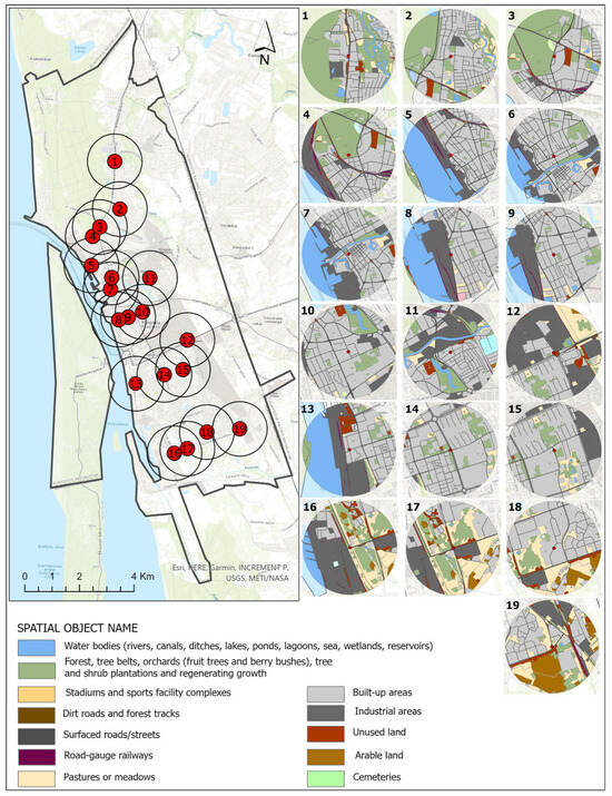
Figure 3.
Land use patterns within 1 km buffers around NO2 monitoring sites in Klaipėda.
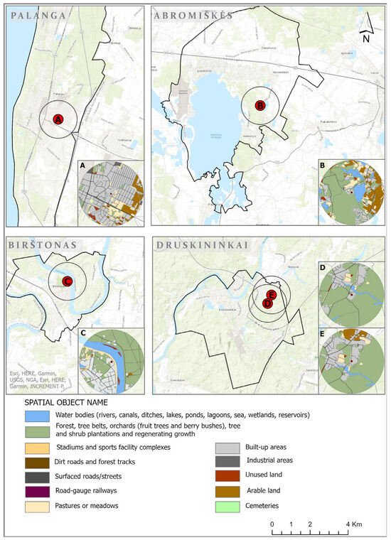
Figure 4.
Land use patterns within 1 km buffers around NO2 monitoring sites in Lithuanian resort towns.
Figure 3 illustrates the spatial layout of all 19 NO2 sampling sites across Klaipėda’s urban area, along with their surrounding buffer zones. The central map displays site locations overlaid on the city’s base map, while the adjacent inset maps depict detailed land use structure within each buffer. These insets reflect the proportion and spatial arrangement of various land cover types—such as built-up areas, transport corridors, industrial zones, and green spaces. Although some buffer zones partially overlap due to the uniform 1 km2 area defined around each site, each buffer is analyzed independently. This means that the same spatial objects, such as streets or corridors, may contribute to more than one site’s index calculation if they fall within multiple buffers. This approach ensures methodological consistency and allows local morphological differences—such as the presence of forests in one buffer but not another—to be fully captured.
Figure 4 presents the monitoring locations in resort and therapeutic towns measured during the 2024 campaign. The same spatial analysis approach was applied, enabling consistent comparison of land use composition between the urban and resort settings.
In this study, land use classification for each sampling site was based on official national GIS datasets, providing spatially encoded feature codes and delineated land cover types. Cadastre data and information are collected and stored by the state using the Lithuanian coordinate system, LKS-94, and in the Lithuanian state altitude system, LAS07. To ensure consistency across all locations, the analysis included only the principal land use categories that demonstrated substantial coverage within the defined buffers. These dominant classes were consistently observed across all 24 sites—19 in Klaipėda and 5 in resort towns—and are presented in Table 1, together with their corresponding GIS feature codes.

Table 1.
Land use categories and corresponding GIS feature codes used in buffer analysis.
2.2.2. Statistical Correlation Analysis
To explore how land use categories relate to ambient air pollution, a statistical analysis was conducted to quantify their associations with nitrogen dioxide (NO2) concentrations. Specifically, Pearson correlation analysis was applied to assess the linear relationships between the proportion of each land cover type within a buffer zone and the measured NO2 levels. This method is commonly used in environmental and air quality studies to identify statistically significant spatial relationships between land-based variables and atmospheric pollutants [12].
Even though Pearson correlation is a widely applied method in environmental sciences for identifying spatial associations between land surface characteristics and pollutant concentrations, in this study, it served not as an endpoint but as a foundation for constructing a more comprehensive spatial assessment tool. Recognizing the limitations of correlation alone—particularly its inability to capture composite spatial susceptibility—this analysis advanced toward the development of an integrative metric. To support this next step, all land cover types were grouped into functional categories, which were subsequently used for both the statistical analysis and the final index construction.
- (i)
- Urbanization: Includes built-up areas (general residential and mixed-use urban structures) and industrial and commercial areas (codes: pu0, pu3).
- (ii)
- Transport infrastructure: Includes paved roads and urban streets, railway lines, and forest roads (codes: gt12, gt14, gt2, gt18, gt15, gt16).
- (iii)
- Green and natural areas: Includes forests, tree rows, orchards, green urban areas, shrub vegetation, arable land (cultivated fields), pastures and grasslands, and surface water bodies (rivers, lakes, ponds, reservoirs, etc.) (codes: mj0, ms0, ms4, sd15, vk1, sd11, sd2, hd1, kd2, hd3, hd4, hd5, hd6, hd9).
- (iv)
- Others: Includes abandoned or unused land and cemeteries (codes: sd4, vp1), which were excluded from the functional grouping due to their ambiguous ecological roles and negligible direct anthropogenic emissions.
This functional grouping served as the basis for the subsequent statistical analysis and for developing the composite pollution pressure index.
2.2.3. Development of LUPP and PLUPP Indices
To more effectively evaluate how the structural composition of urban and semi-natural landscapes contributes to ambient air pollution, independently of direct emission inventories or population data, a composite indicator—Land Use Pollution Pressure (LUPP) index—was introduced. This index was designed to quantify the theoretical predisposition of an area to pollution, drawing on the land cover types within each site’s buffer zone. The results were calculated by applying this formula.
LUPP = α1⋅Urbanisation + α2⋅Transport − α3⋅GreenAreas; (i) α1 = 0.343 (urbanization R2); (ii) α2 = 0.230 (transport infrastructure R2); (iii) α3 = 0.359 (green/natural areas R2)
The same land use grouping used for the correlation analysis was applied here to construct the index, defining three functional domains based on their environmental role: (i) Urbanization (built-up and industrial areas); (ii) Transport Infrastructure (paved roads, railways, forest tracks); (iii) Green and Natural Areas (forests, meadows, arable land, water bodies). Each land use component was weighted using its explained variance (R2) from the regression analysis, reflecting its relative contribution to NO2 concentrations across the 24 observation sites.
This formulation allows for an indirect estimation of environmental pressure. A higher LUPP score suggests a land cover configuration that is likely to produce or sustain elevated pollution levels, due to the dominance of urban and transport-related surfaces and the relative scarcity of vegetated or natural buffers. Conversely, negative or low LUPP values indicate areas where green infrastructure may be sufficiently dominant to mitigate pollution effects.
While the LUPP index offers a useful estimation of spatial pollution potential based solely on land use structure, it does not account for differences in population exposure, which are critical for understanding actual public health risk. To address this limitation, a population-weighted extension—Population-Weighted Land Use Pollution Pressure (PLUPP)—was introduced. This novel refinement integrates demographic variables into the spatial pollution model, allowing the assessment to move from theoretical susceptibility toward actual exposure burden.
PLUPP was calculated only for Klaipėda due to stable residential patterns; resort towns with transient populations were excluded.
To prepare the population exposure dataset required for the PLUPP index, a spatial overlay between circular buffer zones and national population grids was conducted. Each of Klaipėda’s 19 monitoring sites was surrounded by a 1-km Euclidean buffer, representing the assumed area of exposure. However, the demographic dataset—structured as fixed 1 km2 statistical grid cells—did not align perfectly with the circular buffers. Many grid cells were only partially intersected by a given buffer. Simply summing populations from these cells would have overestimated the actual number of individuals present within each buffer zone.
To address this, we applied a proportional area-weighting approach: for each intersected grid cell, we calculated the share of its area (shape area 2) that overlapped the buffer relative to the cell’s total area (shape area 1). This ratio was used to adjust the total population within each intersected cell:
If a grid cell was entirely within the buffer, the full population was included. Otherwise, only a proportional share was counted. This adjustment assumes a uniform spatial distribution of population within each cell.
Similarly, population by age group was proportionally scaled using the same ratio:
All adjusted values were aggregated by stop, resulting in a harmonized dataset of total and age-specific population exposure within a 1 km buffer around each air pollution monitoring station. Based on this refined demographic and spatial dataset, two composite indices—Total PLUPP (hereafter referred to as PLUPP) and vulnerability-weighted PLUPP (PLUPPvw)—were developed to evaluate air pollution sensitivity at the urban population level.
PLUPP = (NO2 + Urban + Transport) × (POP + 2x (Children + Elderly)) − Green areas
In this study, NO2 represents mean annual concentration (µg/m3), urban, transport, and green areas are land cover extents in square kilometers (km2) within each 1 km buffer; POP, children, and elderly are absolute population counts (persons). While these variables have different units, they were intentionally aggregated without prior standardization to capture the combined absolute pollution load, land use intensity, and population exposure. The resulting composite index was then normalized to a unitless 0–1 scale to ensure comparability across sites. Children and the elderly in the PLUPP index were assigned double weight to account for their increased physiological vulnerability. Studies show that heat-related mortality in the elderly can be up to twice as high as in the general population [13,14], while children exhibit higher exposure per body weight and greater sensitivity to pollutants due to immature detoxification systems [15]. Although the literature does not prescribe a specific multiplier, a weight of 2.0 was selected as a conservative yet illustrative estimate within the observed risk range (typically 1.5–2×), allowing for clear differentiation of these sensitive groups in the index. To balance the pressure component of the index with potential mitigating factors, green areas—known to reduce air pollution and support public health—were subtracted as a compensatory element, reflecting their pollution-reducing and health-protective effects as documented in urban environmental studies [9].
The resulting composite index was then normalized to a 0–1 scale to enable comparison across monitoring locations. This method is particularly useful for comparing urban areas in spatial planning, where identical activities—such as industrial development—may result in significantly different environmental risks due to differences in local population structure, particularly the proportion of sensitive demographic groups such as children and the elderly.
Additionally, a vulnerability-weighted PLUPP (PLUPPvw) was developed to capture the relative exposure risk faced by the average resident, emphasizing areas with a higher share of sensitive age groups and limited green space. Sensitive age groups are included as a proportion of the total population, thus reducing the influence of absolute population numbers on the index value.
Unlike in the Total PLUPP formula, where green space is subtracted as a gross compensatory factor, the PLUPPvw index places green areas in the denominator. This design reflects green infrastructure as a proportional protective factor—meaning that the more green space available for vulnerable-age-group residents, the lower the expected environmental risk. Accordingly, the calculated pressure was divided by the amount of green area (with a small constant ε added to avoid division by zero), capturing relative sensitivity per individual rather than total burden. Children (aged 0–14) and elderly residents (65+) retained double weight in this index as well, ensuring methodological consistency with the Total PLUPP.
To facilitate qualitative interpretation and cross-comparison, both the Total PLUPP and the PLUPPvw index were classified into three ordinal categories: Low, Medium, and High. This classification was based on the tercile (quantile) distribution of the respective index values. Specifically, thresholds were derived from the 33rd and 66th percentiles, dividing the full range of values into three approximately equal segments. The data were normalized to a 0–1 scale. This approach is widely applied in environmental risk analysis and spatial vulnerability assessments as a means to simplify interpretation while preserving the underlying distributional structure [16].
Although both indices enhance the interpretive value of exposure assessments, it is important to acknowledge a key methodological limitation associated with the population data. Since demographic information was sourced from statistical grids, the boundaries of these cells rarely aligned perfectly with the circular 1-km buffer zones used in the analysis. As a result, population counts within each buffer were estimated using a proportional area-weighting method, which calculates the share of each grid cell intersecting the buffer and scales the cell’s population accordingly. This calculation assumes uniform population distribution within each cell, which may not reflect actual settlement density on the ground. Importantly, these indices were designed for a compact, low-relief coastal city with relatively homogeneous meteorological conditions influenced by a maritime climate [17,18,19]. As such, variables like wind dispersion, terrain complexity, and vertical urban form (building height) were not incorporated, as pollutant dispersion is assumed to be relatively even across the study area. The development of the LUPP and PLUPP indices represents a novel methodological contribution. These indices allow for the identification of high-risk areas by jointly assessing spatial pollution potential and demographic vulnerability.
3. Results
3.1. Klaipėda’s Air Quality and Green Areas: A Resort Comparison
This study compared NO2 concentration levels measured during the summer of 2024 in Klaipėda city and Lithuania’s major resort areas. The results revealed significant differences (Figure 5). In resort areas, NO2 levels were as follows: Druskininkai (UPA Medical Centre—5.56 µg/m3), “Eglė” Sanatorium in Druskininkai—5.92 µg/m3, “Eglė” Sanatorium in Birštonas—8.20 µg/m3, Abromiškės Rehabilitation Centre—3.88 µg/m3, and Palanga (residential area)—6.44 µg/m3. In Klaipėda, NO2 concentrations were substantially higher at key urban sites: Port Area—32.09 µg/m3, Transport Hub—37.34 µg/m3, and Residential Area—12.55 µg/m3. All values represent mean concentrations measured during the two-week summer campaign in August 2024, corresponding to the average over the entire measurement period.
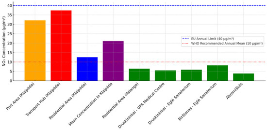
Figure 5.
Comparative analysis of NO2 pollution levels (µg/m3) in Klaipėda and resort areas.
A direct comparison revealed that the NO2 concentration at Klaipėda’s transport hub was approximately seven times higher than the lowest NO2 value observed in Abromiškės Rehabilitation Centre (Figure 5). Even the residential area in Klaipėda exhibited approximately twice the NO2 levels compared to Palanga’s residential zone. Moreover, variability in NO2 levels within Klaipėda was significantly greater than in resort areas. In the city, NO2 concentrations during the summer of 2024 ranged from approximately 12.55 µg/m3 to 37.34 µg/m3, whereas in the resort areas, concentrations remained narrowly confined between 3.88 and 8.20 µg/m3. This strong variability within Klaipėda indicates pronounced spatial heterogeneity, reflecting the uneven distribution of emission sources such as heavy traffic, port activities, and residential patterns. In contrast, the low variability in resort areas suggests a more uniform air quality environment, typical of less industrialized and less urbanized settings. These results highlight how different land use types—dense transport infrastructure, industrial port zones, and residential areas—directly shape NO2 levels, supporting the link between land cover and local air quality.
To provide a broader context for interpreting the 2024 summer measurements, we also referred to seasonal NO2 data collected throughout 2023 from 19 locations across Klaipėda. While the summer 2024 measurements at selected urban points and resorts are directly compared in the figure, the citywide 2023 mean offers an important background reference for understanding the general air pollution burden in Klaipėda.
Globally, annual mean NO2 concentrations in urban areas typically range between 20 and 90 µg/m3 [20]. In Klaipėda, the calculated annual mean NO2 concentration based on 2023 passive measurements reached approximately 21.1 µg/m3, positioning the city at the lower end of the global urban pollution range. However, despite this relatively low citywide average, NO2 levels vary greatly between different urban zones, highlighting how local land use intensity and functional zoning can create significant pollution contrasts within the same city. The results, presented in Figure 5, reveal pronounced spatial disparities. In particular, Klaipėda’s Transport Hub (37.34 µg/m3) and Port Area (32.09 µg/m3) clearly fall within the high-risk zone, exceeding the 30 µg/m3 and approaching the EU legal limit. Meanwhile, Klaipėda’s residential zone is 12.55 µg/m3. This finding underlines the importance of not relying solely on citywide averages when evaluating air quality risks. Local land use configurations—such as the concentration of transport corridors, industrial areas, and limited green buffers—can create localized hotspots that pose disproportionately higher exposure risks. Therefore, understanding these intra-urban patterns is essential for developing targeted pollution mitigation strategies that go beyond generic city-level indicators.
In contrast, NO2 concentrations across all surveyed resort areas—including Druskininkai, Birštonas, Abromiškės, and Palanga—remain well below the 10 µg/m3 threshold. These locations reflect environments where land use composition—with more green and recreational zones—naturally maintains lower NO2 levels. This demonstrates the practical relevance of considering land cover configuration in urban air quality management.
3.2. Land Use Analysis and Its Relationship with Nitrogen Dioxide (NO2) Pollution
To examine how different types of land use are related to environmental pollution, a GIS-based spatial analysis was conducted. Around each air quality monitoring site, a 1 km radius buffer zone was established (resulting in an area of approximately 3.1416 km2). Within these zones, concentrations of nitrogen dioxide (NO2) and particulate matter (PM) were measured, and land cover characteristics were extracted. However, as explained in the methodology section, PM concentrations in the resort towns were below detection limits, resulting in an insufficient number of observations for reliable statistical inference. Consequently, only NO2 data were used in the correlation analysis to maintain a consistent dataset across all 24 locations and to ensure the statistical validity of Pearson correlation coefficients.
The analysis included the following land use categories: paved roads and streets, forest roads, railway lines, surface water bodies, forests and green spaces (including orchards and shrubbery), built-up urban areas, industrial and commercial zones, arable land, pastures and meadows, abandoned or unused land, and cemeteries. These categories were derived from thematic GIS layers (Table 1) and reflect a comprehensive spectrum of both urban and natural land cover types.
Each land use type was quantified as an absolute area (in km2) within the buffer zone and statistically analyzed to assess its correlation with measured pollution levels. Pearson correlation coefficients (r) and corresponding p-values were calculated to evaluate both the strength and significance of these associations (Table 2).
Table 2.
Pearson correlation coefficients and R2 values assessing the association between land use types and nitrogen dioxide (NO2) concentrations.
The Pearson correlation analysis revealed a range of positive and negative associations between land use types and measured NO2 concentrations across all 24 monitoring sites. Among the strongest positive correlations was that with industrial and commercial areas (r = 0.65, p = 0.001), which was statistically significant at the 0.01 level. This finding is consistent with earlier studies [21] reporting a similarly strong relationship (r ≈ 0.7) between industrial land use and NO2 levels within urban buffer zones. In this study, the corresponding R2 value for industrial land use was 0.421, indicating that this category alone explains over 42% of the variation in NO2 concentrations across the measured sites.
A similarly strong but negative and statistically significant relationship was observed for forests, orchards, green urban areas, and shrub vegetation (r = −0.66, p = 0.001), indicating that greener environments were associated with lower NO2 levels. These results align with other research [22] showing that vegetated and natural areas can significantly reduce NO2 exposure in urban settings. The R2 value of 0.43 makes green areas the most statistically powerful single land use predictor in this dataset, highlighting their role in mitigating air pollution.
Moderate correlations were also identified. Paved roads and urban streets exhibited a significant positive correlation (r = 0.43, p = 0.037, R2 = 0.183), suggesting that traffic infrastructure contributes to local NO2 concentrations. Conversely, forest roads showed a significant negative correlation (r = −0.416, p = 0.043, R2 = 0.173), possibly reflecting the spatial separation such infrastructure provides from densely trafficked areas.
Other land use types demonstrated weaker or non-significant correlations. For instance, railway lines showed a positive correlation (r = 0.30, p = 0.150), but this relationship did not reach statistical significance. Arable land exhibited a negative association (r = −0.25, p = 0.233, R2 = 0.064), suggesting a potential mitigating effect, though also not statistically significant.
Some land use categories, such as cemeteries, abandoned or unused land, and pastures and grasslands, showed very weak or negligible correlations with NO2 concentrations (R2 < 0.02, p > 0.5), indicating minimal predictive value. Built-up urban areas (r = 0.24, p = 0.255) and surface water bodies (r = 0.19, p = 0.382) showed slightly stronger correlation coefficients compared to other weakly correlated categories, though these associations were not statistically significant, indicating limited predictive value.
It should be noted that the correlation analysis is based on 24 monitoring sites, which offers a moderate sample size for detecting statistical relationships. While this number allows for the identification of meaningful associations—particularly those with stronger effect sizes—smaller or borderline correlations may still fall short of statistical significance.
To mitigate these constraints and gain a clearer picture of overall spatial influence, the analysis shifted from individual predictors to broader landscape-level groupings, which are described in the Methodology section and illustrated in Figure 6. This dimensionality reduction—from eleven detailed variables to a few functional categories—not only enhanced model stability and reduced multicollinearity, but also reflected how land use operates as a structured system rather than as disconnected fragments. This strategy aligns with best practices in spatial modeling under small-sample conditions [23].
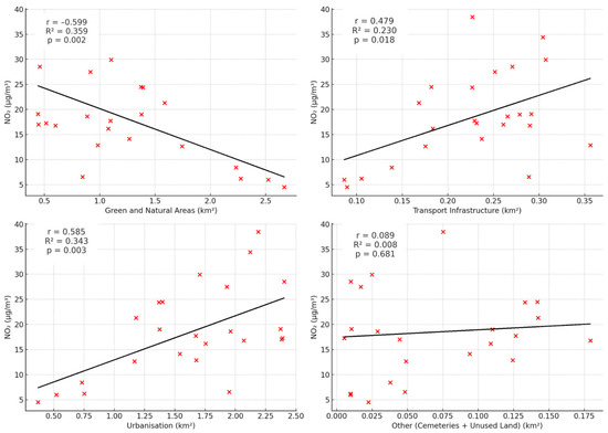
Figure 6.
Linear relationships between grouped land use domains and nitrogen dioxide (NO2) concentrations.
To visualize the strength and direction of the relationships between aggregated land use categories and NO2 concentrations, four scatterplots were created (Figure 6). Each plot presents the linear relationship between the area (in km2) of a functional land use grouping and the corresponding NO2 levels measured at the 24 monitoring sites.
This analysis explores the relationship between nitrogen dioxide (NO2) concentrations and four aggregated land use categories: urbanization, transport infrastructure, green and natural areas, and others. These groupings were developed to reflect broader functional roles of land use while minimizing multicollinearity and statistical noise associated with individual variables.
Urbanization shows a moderate to strong positive association with NO2 concentrations. The regression analysis produced an R2 value of 0.343, indicating that approximately 34% of the variation in NO2 levels across the study sites can be explained by the combined share of built-up and industrial land. While this is lower than initially expected, it remains statistically significant (p = 0.003), confirming that dense urban structures contribute meaningfully to elevated pollution. This result aligns with existing research demonstrating that urban and industrial zones concentrate vehicular traffic, heating, and stationary emission sources, reinforcing NO2 accumulation [24].
Transport infrastructure also demonstrates a moderate positive relationship (R2 = 0.230, p = 0.018). This group includes paved roads, railway lines, and forest roads—features that differ substantially in traffic volume and emission potential. While paved roads represent high-emission corridors, forest roads often carry minimal traffic, and some railway lines may operate under electric systems. As a result, the group’s explanatory power is diluted by the inclusion of low-emission infrastructure. This limitation is well-documented in land use regression (LUR) literature, where traffic counts significantly enhance predictive power [25].
Green and natural areas show a strong and statistically significant negative association with NO2 concentrations (R2 = 0.359, r = −0.599, p = 0.002), consistent with existing evidence that vegetation helps mitigate pollutants via deposition, dispersion, and microclimatic effects. While this aggregated group includes highly effective land types such as forests and urban greenery, it also includes surface water bodies, which showed weak correlation with NO2 individually (r = 0.172, R2 = 0.030). Water bodies, unlike vegetation, do not actively absorb NO2, which likely explains the reduction in overall explanatory power. These findings align with previous research [9], which demonstrated that tree canopies filter pollutants via stomatal uptake and surface deposition, while open water plays no direct role in air purification.
The “Others” category, comprising abandoned land and cemeteries, did not demonstrate any statistically meaningful relationship with NO2 levels (R2 = 0.008, p = 0.735). These land types are structurally present in the landscape but likely lack any strong causal link to either pollutant emission or mitigation. Their relatively small extent and ambiguous ecological function may explain their negligible statistical influence.
In summary, grouping land use categories helped identify meaningful spatial patterns in NO2 variation. Compared to individual land use types, these aggregated variables offered clearer insight into the structural drivers of pollution. Notably, although vegetation-based land uses—especially forests—are often assumed to reduce NO2 concentrations, this association may reflect spatial displacement rather than true pollutant removal. In other words, areas with high forest cover often coincide with less intensive development, implying lower emissions from transport or industry, rather than active NO2 uptake by vegetation.
Scientific evidence supports this interpretation: studies have shown [9] that trees absorb only limited amounts of NO2, and that their role in air purification is minor compared to emission reduction strategies. Therefore, the observed negative correlations between NO2 and green land cover should be interpreted as indicators of less built-up intensity, rather than a direct mitigation effect. In contrast, urbanized areas and transport infrastructure remain the most consistent predictors of elevated NO2 concentrations.
3.3. Land Use Pollution Pressure (LUPP) Index
Understanding how land use configuration influences air pollution pressure is essential for spatial planning and environmental risk assessment. Land use plays a critical role in shaping the spatial distribution of pollutants, particularly in urban and peri-urban environments. To systematically capture this relationship, we developed a composite indicator—the Land Use Pollution Pressure (LUPP) Index—which estimates pollution potential based solely on land cover characteristics.
Before introducing the index formulation, it is important to distinguish this approach from conventional Land Use Regression (LUR) models. LUR is a widely used method for estimating air pollutant concentrations at unsampled locations. These models typically incorporate multiple spatial predictors, such as traffic intensity, elevation, population density, and meteorological variables [7,24]. While powerful, LUR models depend on the availability of high-resolution, multi-source datasets and require empirical calibration based on a limited number of air quality monitoring sites.
These requirements often constrain LUR applicability in data-scarce settings, especially during the early stages of spatial planning or in regions with limited environmental infrastructure [26]. Furthermore, LUR models are primarily optimized for spatial prediction, rather than for interpreting structural environmental relationships, which limits their utility when the objective is explanatory insight or comparative diagnostics across land units.
In contrast, the LUPP index was developed as a novel, simplified, and static structural indicator of air pollution pressure derived exclusively from land cover data. Rather than estimating pollutant concentrations, the LUPP index captures the inherent pollution-driving potential of land use configurations. It is grounded in empirically observed relationships from a fully monitored dataset of 24 observation sites, ensuring that each land use component reflects its real-world contribution to NO2 variation.
However, it is crucial to acknowledge the conceptual limitations of the LUPP index. First, the index does not account for vertical urban structure—such as building heights or floor area ratios—which can significantly influence pollutant dispersion and accumulation. Second, traffic volumes, population densities, and specific emission intensities are not included in the formulation. As a result, the index may underestimate pollution pressure in dense vertical developments (high-rise city centers) and overestimate it in low-density industrial areas where land use alone suggests high impact. These limitations highlight that LUPP should be interpreted as a structural proxy for land use pressure, not as a direct predictor of emissions or exposure levels.
Despite these constraints, the index offers several practical advantages. It enables spatial comparisons across sites using only land cover data and supports planning processes by identifying zones with the greatest structural pollution potential. It is particularly valuable in data-poor regions or early-stage assessments.
It is also important to emphasize that the LUPP index was calibrated using land use data and NO2 measurements from 24 monitoring sites in Lithuania, covering a diverse spectrum from urbanized zones (Klaipėda) to resort towns with extensive green infrastructure (Birštonas, Druskininkai, Abromiškės). The resulting R2 weights are therefore context-specific, reflecting the land cover–pollution relationships characteristic of this regional setting.
For application in other regions or countries, local recalibration is required. Specifically, local NO2 measurements and land use data must be used to generate new regression coefficients (R2) tailored to the geographical, morphological, and infrastructural context of the area under analysis.
Figure 7 visualizes LUPP values across the 24 observation locations. Sites are color-coded according to index polarity: positive values (red) indicate land cover configurations structurally predisposed to higher pollution pressure due to the dominance of urban and transport surfaces. Conversely, negative values (green) reflect areas dominated by green and natural land types, which exert a buffering effect and generally represent low-risk environments.
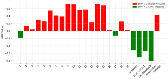
Figure 7.
Land Use Pollution Pressure (LUPP) index values across monitoring sites, indicating spatial distribution of structural land use pressure.
The results show that several monitoring locations in Klaipėda—particularly stations 9, 10, 14, and 15—exhibit high LUPP values due to dense residential development and nearby transport infrastructure. However, these locations do not correspond to the highest NO2 concentrations, highlighting a key nuance: LUPP captures structural susceptibility to pollution, not necessarily current emission intensity (Figure 8). Residential zones tend to show elevated LUPP due to built-up density and limited vegetated buffers, even if direct emission sources are moderate.
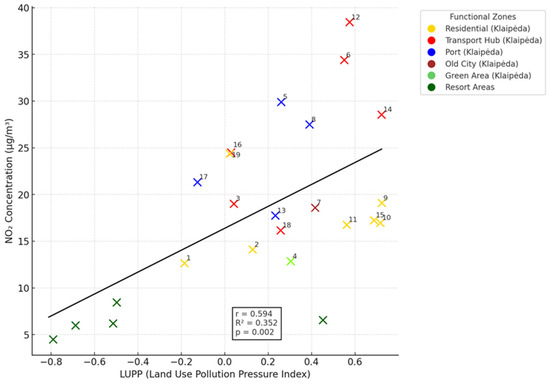
Figure 8.
NO2 concentration in relation to Land Use Pollution Pressure index.
This finding aligns with studies on the urban canyon effect, which demonstrate that pollutants can accumulate and persist in densely built areas due to restricted air circulation. Previous research [27] shows that street canyons with high building density and limited ventilation can retain pollutants for longer periods, especially in residential areas where emissions are moderate but dispersion is constrained.
The classification of monitoring stations into functional zones—such as residential, port, transport, and resort areas—was based on prior spatial analysis of Klaipėda’s urban structure and emission sources [11]. This classification enabled the evaluation of land use-specific pollution pressure in a consistent and spatially meaningful way.
By contrast, resort towns such as Abromiškės, Birštonas, and Druskininkai 1–2 display strongly negative LUPP values, consistent with their abundant green space, low urban footprint, and minimal transport presence. These areas exhibit both low structural pressure and low NO2 levels, reinforcing the buffering capacity of natural landscapes.
A particularly illustrative case is Palanga, which currently exhibits low NO2 concentrations but has a positive LUPP value—higher than several locations in Klaipėda. This apparent contradiction underscores LUPP’s strength as a forward-looking indicator: it does not measure pollution directly but evaluates the landscape’s structural vulnerability. In Palanga, a moderate extent of urban land and a relatively limited vegetated buffer contribute to its heightened LUPP, suggesting increased susceptibility should development or traffic intensify.
Station 1, located in Dragūnai district, exemplifies low structural pressure within Klaipėda: its relatively low LUPP is supported by substantial green infrastructure, as confirmed by previous studies identifying it as one of the city’s cleanest residential zones. Similarly, Station 17 and the northernmost site in Klaipėda also show negative LUPP scores, reflecting a favorable balance of natural land cover and reduced urban or transport impact.
Thus, the LUPP index acts as a land use-based early warning system, enabling planners to anticipate where environmental pressure may emerge—not based on emissions alone, but based on the landscape’s inherent capacity to concentrate or dissipate pollution. By integrating land use proportions with regression-derived weights (R2), the index provides a scalable and interpretable tool for environmental risk assessment, particularly in data-scarce contexts. This structural susceptibility framework helps explain why built environments remain a central concern for air quality even when real-time emissions are not extreme.
Figure 8 reinforces the explanatory power of LUPP. The scatterplot shows a statistically significant positive correlation between LUPP and NO2 (r = 0.594, p = 0.002), with R2 = 0.352. This indicates that over one-third of the variation in NO2 levels can be attributed to land use structure alone. While the relationship is not deterministic—reflecting the role of emission intensity and meteorological factors—it confirms that areas with higher LUPP values are generally more prone to elevated NO2 concentrations.
In summary, LUPP is not only a theoretically grounded index but also an empirically validated predictor of structural pollution susceptibility. Its value lies in its ability to bridge land use data with air quality insights, offering a scalable tool for spatial planning and environmental risk screening.
Unlike a raw aggregation of land cover types, LUPP incorporates regression-derived R2 weights, which reflect the measured influence of each land use category on NO2 concentrations. This weighting system adds critical nuance: without it, the index would treat all land use components as equally impactful—failing to account for the empirical strength of urbanization, transport infrastructure, or green areas in shaping pollution potential. The result would be a less informative, uncalibrated spatial overlay.
Notably, the integration of R2 weights ensures that land uses are not simply counted, but valued according to their empirically measured influence on NO2 concentrations. For example, although roads and transport zones are often assumed to drive pollution, their lower R2 compared to urbanization reflects that, without surrounding built-up density, their contribution to NO2 variability is limited. This prevents overestimating structural pressure in open or sparsely developed transport corridors.
3.4. PLUPP (Population-Weighted Land Use Pollution Pressure): Sensitivity Indices for Air Pollution Exposure Assessment in Klaipėda
To better understand the spatial distribution of environmental risk across Klaipėda, the PLUPP index was applied as an integrative measure of land use-related pollution pressure weighted by population characteristics. While the methodology behind PLUPP has been detailed earlier, this section focuses on its application and interpretation—highlighting how urban form, pollution levels, and population vulnerability intersect in space. By combining physical environmental data (NO2 levels, urbanization, transport infrastructure, and green areas) with demographic structure (population size and age sensitivity), PLUPP enables a more socially grounded assessment of air pollution risk than land cover data alone. The results offer insight into both cumulative exposure burdens (total PLUPP) and relative vulnerabilities (vulnerability-weighted PLUPP) across monitoring zones, helping to identify where environmental inequalities may emerge due to combined spatial and demographic pressures.
While both indices serve to highlight vulnerability to urban air pollution, they are designed to answer slightly different questions. The Total PLUPP reflects the cumulative environmental pressure, which depends on the absolute number of residents, the number of vulnerable age groups, and the intensity of urban land use. This means that the higher the population (especially children and the elderly), the higher the NO2 levels, and the lower the amount of green space, the greater the overall risk in a given area. This index primarily emphasizes quantity—population concentration and the total burden of exposure.
In contrast, the vulnerability-weighted PLUPP assesses the structural vulnerability of an area, which is determined not by the total number of residents, but by the relative share of vulnerable groups (children and the elderly as a proportion of the total population) and the amount of green space within the buffer. It highlights how a sensitive demographic structure, combined with limited access to greenery, increases territorial vulnerability—even in areas with a small total population.
Table 3 represents how the Total PLUPP and PLUPPvw indices vary across monitoring sites, highlighting areas of concern and potential targets for intervention. To aid interpretation and enable meaningful comparison across locations, both indices were normalized to a 0–1 scale and classified into three ordinal categories—Low, Medium, and High—based on tercile thresholds.
Table 3.
Classification of total and vulnerability-weighted PLUPP indices across measurement stations.
As shown in Table 3 most of the analyzed monitoring stations exhibit alignment between the total PLUPP and PLUPPvw, as both classify the stations into the same sensitivity category—low, medium, or high. This consistency suggests that, in many territories, the structural environmental burden and individual vulnerability are proportionally distributed, resulting in similar categorizations of collective and individual risk.
However, five monitoring stations deviate significantly from this pattern, revealing differing mechanisms of risk distribution. In three stations—11, 16, and 8—the PLUPPvw is higher than the total PLUPP, indicating that although cumulative environmental pressure may be low, the individual-level sensitivity is relatively high. This discrepancy is typically driven by two main factors: (1) a high proportion of sensitive population groups (children and elderly) and (2) limited green space, which in the PLUPPvw formula functions as an ecological buffer.
In station 11, the proportion of sensitive residents reaches approximately 33%, while the green space area is minimal—only 0.599 km2. The area also exhibits intense urban development pressure. Although the cumulative environmental load appears moderate, constrained ecological conditions elevate individual vulnerability. In station 16, the demographic sensitivity is slightly lower (30%), yet green space availability is the lowest among all stations—just 0.548 km2. This lack of ecological amortization emerges as the principal driver of the higher per capita index. However, the total PLUPP remains low, primarily due to the small overall population within the buffer zone, which limits the cumulative exposure burden despite structural land use pressure. In station 8, the proportion of children and the elderly is nearly 35%, and green space measures 0.911 km2. Although this is higher than in stations 11 and 16, it remains insufficient considering the elevated NO2 levels and urban intensity. These factors together result in a higher vulnerability-weighted than total pressure. Therefore, more green space would be needed in this territory to offset the impact of high NO2 concentration and a vulnerable population composition. Green spaces play an essential role in mitigating air pollution by capturing airborne particles and absorbing gaseous pollutants, thus reducing residents’ exposure to harmful emissions [28].
The opposite trend is observed in stations 3 and 18, where the PLUPPvw index falls into a lower category than the total PLUPP. In station 3, the share of sensitive groups approaches 40%, yet the area benefits from one of the highest green space values among all stations—1.377 km2. This strong ecological buffering effectively lowers individual vulnerability despite moderate cumulative pressure. In station 18, the total population is as high as 24,902, and the share of vulnerable groups reaches 37%. However, the availability of 1.078 km2 of green space helps distribute environmental stress across a large population base, significantly reducing per-person sensitivity even under high total exposure. This shows that a high proportion of sensitive residents can be mitigated by sufficient green infrastructure in the area. Thus, while the total sensitivity increases due to the large population, the extensive green space reduces the pressure experienced by each individual, especially for the elderly and children.
These differences reflect the fundamental structural distinctions between the two indices. The total PLUPP index primarily captures the absolute demographic load and structural land use intensity—highlighting where population size, vulnerable group concentration, and urban density co-occur. In contrast, the PLUPPvw index emphasizes the ecological and social context of individual exposure, where green space availability per resident becomes a key mitigating factor. As such, green areas act as a moderating influence on individual sensitivity—even in zones of high environmental pollution, the impact on residents may be mitigated if surrounding ecological conditions provide sufficient compensation. As Briggs underscores, exposure to environmental hazards must be evaluated not only in terms of spatial concentration but also in relation to population characteristics and ecological mitigation capacity [5].
The initial results (Figure 9) show a strong association between LUPP values and the PLUPPvw, with a coefficient of determination (R2) reaching 0.70. This indicates that as much as 70% of the variation in individual sensitivity to air pollution can be explained solely by land use structure. These findings underscore the potential of the LUPP index as a proxy indicator of structural environmental vulnerability, particularly in contexts where detailed demographic or transport data are unavailable.
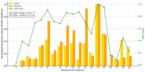
Figure 9.
Normalized total PLUPP and PLUPPvw indices across air pollution measurement stations in Klaipėda, compared to the LUPP index.
The strong correlation between LUPP and PLUPPvw primarily stems from the fact that both formulas are highly responsive to the green space component. In the LUPP index, green areas carry the highest weight among all variables (α3 = 0.359)—greater green space reduces overall structural pressure. Meanwhile, in the PLUPPvw formula, green space is placed in the denominator, so a smaller total green area within the buffer increases the index value. In practice, buffers with scarce greenery—especially if they also have a high share of vulnerable age groups—appear more sensitive. This structural design leads to high values in both indices in territories where green space is limited. In other words, a lack of greenery increases vulnerability at both the structural and individual levels. As noted by Kabisch and Haase (2014), urban green areas not only serve as physical barriers to air pollutants but also provide ecosystem services that mitigate health risks [29]. Therefore, their inclusion in both indices—as a subtractive factor in LUPP and as a denominator in the PLUPPvw formula—is theoretically justified.
In contrast, the total sensitivity index (Total PLUPP) shows only a moderate correlation with LUPP (R2 = 0.43). This difference suggests that PLUPP is more influenced by the absolute number of residents and sensitive population groups (children, elderly) than by land use structure. Unlike LUPP, which captures horizontal territorial pressure, PLUPP can also reflect vertical residential density (e.g., high-rise buildings), a factor not accounted for in the LUPP index.
To better understand how these relationships manifest at the city level, the case of Klaipėda provides a concrete example of spatial disparity in environmental vulnerability. Among all monitoring stations, station 14 in Klaipėda stands out as the most structurally and individually vulnerable area. It exhibits the highest values in all three indicators: LUPP, Total PLUPP, and vulnerability-weighted PLUPP. This convergence suggests a cumulative exposure scenario in which urban structure, demographic composition, and environmental conditions jointly amplify vulnerability. High urban intensity, dense transport infrastructure, low green space per resident, and a high share of sensitive population groups (e.g., children and elderly) characterize this location. Such alignment across structural and per capita indices reinforces the station’s classification as a high-risk zone. This pattern is particularly important in the context of urban planning and public health policy, as it illustrates how the overlapping of multiple environmental stressors and socio-demographic factors can lead to hotspot formation. The case of station 14 may serve as a prototypical example of compound vulnerability, where interventions must target not only emission reduction but also improvements in spatial equity—such as increasing green infrastructure in densely populated or demographically sensitive zones.
Furthermore, contrasting sensitivity profiles can be observed in stations 1 and 16, which represent opposite ends of the sensitivity spectrum. Station 16 has the lowest Total PLUPP value (normalized = 0), suggesting minimal cumulative pressure in absolute terms. However, the PLUPPvw index in this station is non-zero, reflecting notable individual vulnerability. This is largely due to extremely limited green space (0.548 km2), which offers insufficient ecological buffering at the resident level, despite the area’s low population count. In contrast, station 1 has the lowest PLUPPvw index (normalized = 0), indicating minimal individual exposure risk. Nevertheless, its total PLUPP value is non-zero, driven by a higher cumulative exposure burden due to the absolute number of residents in the buffer zone.
These examples demonstrate that both indices—Total PLUPP and vulnerability-weighted PLUPP—are essential for capturing different dimensions of environmental vulnerability. While Total PLUPP highlights cumulative environmental pressure across the general population, PLUPPvw uncovers disparities tied to demographic sensitivity and the unequal distribution of green infrastructure. Low population density does not necessarily equate to low vulnerability if sensitive groups are present and ecological buffers are lacking. Therefore, combining these two indices provides a more comprehensive understanding of exposure dynamics and supports better-informed decisions in urban environmental governance and spatial justice.
3.5. Land Use Change Simulation Modeling: Assessing Impacts on Urban Environmental Pressure
To assess how green space reduction and industrial expansion could impact environmental vulnerability in the study area, a land use change simulation was conducted. Urban land use transformations, even when moderate in scale, can lead to non-linear and spatially heterogeneous effects on environmental vulnerability. For example, the development of new commercial infrastructure at the expense of green areas can exacerbate local exposure to air pollution, reduce ecological buffering capacity, and amplify risks for sensitive population groups. Such structural shifts are particularly relevant in areas already experiencing high environmental load or demographic vulnerability.
To explore the potential impacts of future urban development, a scenario-based sensitivity analysis was conducted. The model simulates a hypothetical situation in which urbanization and transport infrastructure are each increased by 1%, while the proportion of green areas is reduced by 2% (Figure 10). These modifications were applied proportionally across all observation units, representing a generic intensification of the built environment. Even as a hypothetical model, the scenario helps to identify areas that may be more vulnerable to environmental pressure under intensified urban development. It reveals zones with lower resilience to land use changes and highlights where more targeted attention may be needed—such as enhancing green infrastructure, improving transport systems, or supporting vulnerable communities.
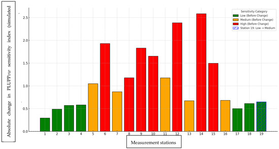
Figure 10.
Deviation from the baseline scenario under simulated land use change, where urbanization and transport infrastructure were each increased by 1%, and green areas were reduced by 2% across all monitoring stations.
This approach provides valuable insight into which urban areas are more likely to experience disproportionate increases in environmental sensitivity under development pressure, regardless of their current vulnerability levels.
Figure 10 presents the absolute change in the vulnerability-weighted PLUPP (PLUPPvw) index under the simulated land use change scenario. The values shown are not normalized and represent raw numerical increases in index scores after the application of the scenario compared to the original baseline. The figure depicts how much the PLUPPvw value increased at each observation unit following the hypothetical changes in urbanization, transport infrastructure, and green space.
The color coding in the figure refers to the sensitivity category of each monitoring station before the scenario was applied. Red denotes sites originally classified as high sensitivity, orange represents medium sensitivity, and green indicates low sensitivity. The color reflects the initial vulnerability level of each area before change, while the bar height indicates the absolute increase in the PLUPPvw index resulting from the land use intensification scenario.
The simulation results (Figure 10) clearly demonstrate that the most environmentally sensitive monitoring stations under the hypothetical land use change scenario are also those that were already classified in the highest sensitivity category prior to the intervention. Specifically, stations 6, 12, and 14—all categorized as high before the simulation—experienced the greatest increases in the PLUPPvw. These zones represent areas where structural exposure to pollution is compounded by demographic vulnerability and limited green space availability, making them particularly susceptible to even moderate intensification of urban development.
In contrast, stations such as 1, 2, 3, 4, and 17, which had been classified as low sensitivity, exhibited only minimal increases in vulnerability. This indicates a relatively robust environmental buffer capacity and lower demographic risk within these zones.
Notably, only one station (No. 19) transitioned between categories—from low to medium—underscoring the non-linear nature of environmental sensitivity and highlighting the potential for significant shifts even in previously low-risk areas when green infrastructure is reduced.
This pattern confirms that areas with high baseline vulnerability are not only at greater risk under current conditions, but are also the most responsive (and fragile) under projected land use transformations. These findings support prioritizing such hotspots in urban planning and environmental mitigation strategies.
4. Discussion
This study provides a focused analysis of air pollution by assessing atmospheric nitrogen dioxide (NO2) concentrations as a key urban air quality indicator. NO2 is strictly regulated due to its direct impacts on human health, mainly originating from vehicle exhaust, energy production, and industrial activities. As most people live in urbanized and industrialized areas, long-term exposure poses significant public health risks.
When comparing pollution between Klaipėda—a persistently polluted industrial seaport city—and low-emission “green” resort areas, a clear disparity emerged with direct implications for environmental quality. Industrial and commercial zones in Klaipėda showed a strong positive correlation with NO2 (r ≈ 0.65), explaining about 42% of concentration variability, while vegetated land covers typical of resort areas showed a strong inverse correlation (r ≈ −0.66), accounting for 43% of variance. This confirms that dense built-up and transport zones raise NO2 levels, whereas greenery acts as a buffer, supporting cleaner air. These results align with international studies which found similar patterns, reinforcing that industrial land use and traffic are strong predictors of NO2, while green coverage consistently reduces it.
Although Pearson correlation analysis was used to identify clear relationships between land use types and measured NO2 levels, this statistical method alone does not quantify the exact magnitude of NO2 changes caused by land use shifts. Therefore, future studies should complement correlation analysis with advanced predictive or influencing-factor models that can simulate different scenarios and more accurately attribute NO2 variation to specific land use dynamics.
In this context, our study’s additional framework goes further by aligning with European Union guidance on ambient air quality assessments. Our study addresses these recommendations through the novel LUPP–PLUPP framework, which combines land use pollution pressure with demographic vulnerability weighting. This integrated approach provides a multi-scalar tool to evaluate urban air pollution exposure more comprehensively than models treating these aspects separately.
Overall, this study demonstrates that understanding local land cover configurations and their demographic context is essential for designing targeted mitigation strategies that go beyond citywide averages and address exposure inequalities within urban areas.
5. Conclusions
The results of the study clearly demonstrate that the spatial distribution of atmospheric nitrogen dioxide (NO2) concentrations in the Klaipėda port city and Lithuania’s inland and coastal resort towns is strongly dependent on land use type. Lower concentrations measured in the resort areas—characterized by more abundant green spaces—confirm that urban vegetation plays a significant role in air quality, as vegetation suppresses pollutant dispersion and acts as a natural filtration mechanism. Comparative analysis revealed distinct air quality differences between the persistently polluted Klaipėda port city and the ‘green’ resort zones.
Statistical relationships between different land-cover categories and NO2 levels revealed the structural role of land use in shaping spatial pollution patterns. These findings suggest that urban planning must not only monitor the expansion of industrial and transportation infrastructure but also actively integrate green-infrastructure elements. Since the majority of the population is concentrated in industrial cities—thereby residing in areas of persistent air pollution—urban planners are advised to increase green space coverage in built-up zones, limit heavy traffic in residential areas, and integrate vegetated buffers around pollution-emitting infrastructure.
The LUPP and PLUPP indices proposed in this study—which combine land use configuration with demographic vulnerability—offer a practical decision support tool: they enable the projection of air quality changes under various land use scenarios and the assessment of exposure risk for different population groups. The indices developed enable the assessment of structural pollution load based on land cover and demographic vulnerability, making them a valuable tool for sustainable urban planning and public health strategy development.
Future research could expand this framework by integrating the vertical dimension of urban structures (building height and volume) to better capture 3D morphological effects on pollution dispersion. In addition, incorporating local atmospheric phenomena—such as sea breeze patterns typical for coastal cities like Klaipėda—could further refine exposure assessments and improve model accuracy.
Author Contributions
Conceptualization A.A.; methodology A.A.; software A.A. and E.V.; investigation, A.A., E.V., R.D. and I.D.; writing and editing, A.A. and I.D.; visualization, A.A. and E.V.; supervision, I.D. and R.D.; All authors have read and agreed to the published version of the manuscript.
Funding
This research has received no external funding.
Institutional Review Board Statement
Not applicable.
Informed Consent Statement
Not applicable.
Data Availability Statement
The data presented in this study are available on request from the corresponding author.
Acknowledgments
We thank the Lithuanian Resorts Association for the opportunity to conduct air pollution measurements within the premises of health resort areas.
Conflicts of Interest
The authors declare no conflicts of interest.
References
- European Environment Agency. Harm to Human Health from Air Pollution in Europe: Burden of Disease Status, 2024; EN HTML: TH-01-24-018-EN-Q; European Environment Agency: Copenhagen, Denmark, 2024; ISBN 978-92-9480-695-6. ISSN 2467-3196. [Google Scholar] [CrossRef]
- Onivefu, A.P.; Imarhiagbe, O. Types of Air Pollutants. In Air Pollutants in the Context of One Health; Springer: Cham, Switzerland, 2024. [Google Scholar]
- Pisoni, E.; Guerreiro, C.; Namdeo, A.; Gonzalez Ortiz, A.; Thunis, P.; Jannsen, S.; Ketzel, M.; Wackenier, L.; Eisold, A.; Volta, M.; et al. Best Practices for Local and Regional Air Quality Management; Publications Office of the European Union: Luxembourg, 2022. [Google Scholar]
- Singh, H. Urban Forests, Climate Change and Environmental Pollution: Physio-Biochemical and Molecular Perspectives to Enhance Urban Resilience; Springer: Cham, Switzerland, 2024. [Google Scholar]
- Briggs, D.J. The use of GIS to evaluate traffic-related pollution. Environ. Health Perspect. 2007, 64, 1–2. [Google Scholar] [CrossRef] [PubMed]
- Beevers, S.D.; Carslaw, D.C. The impact of congestion charging on vehicle emissions in London. Atmos. Environ. 2005, 39, 1–5. [Google Scholar] [CrossRef]
- Hoek, G.; Beelen, R.; de Hoogh, K.; Vienneau, D.; Gulliver, J.; Fischer, P.; Briggs, D. A review of land-use regression models to assess spatial variation of outdoor air pollution. Atmos. Environ. 2008, 42, 7561–7578. [Google Scholar] [CrossRef]
- Dailidiene, I.; Davuliene, L.; Kelpšaite-Rimkienė, L.; Razinkovas-Baziukas, A. Analysis of the climate change in Lithuanian coastal areas of the Baltic Sea. J. Coast. Res. 2012, 28, 557–569. [Google Scholar] [CrossRef]
- Nowak, D.J.; Crane, D.E.; Stevens, J.C. Air pollution removal by urban trees and shrubs in the United States. Urban For. Urban Green. 2006, 4, 115–123. [Google Scholar] [CrossRef]
- Andriulė, A.; Suzdalev, S.; Vasiliauskienė, E.; Dailidienė, I. Air Pollution and Dispersion of Airborne Chemical Elements in Klaipėda Seaport-City. Sustainability 2025, 17, 3834. [Google Scholar] [CrossRef]
- Andriulė, A.; Vasiliauskienė, E.; Rapalis, P.; Dailidienė, I. Air Pollution in the Port City of Lithuania: Characteristics of the Distribution of Nitrogen Dioxide and Solid Particles When Assessing the Demographic Distribution of the Population. Sustainability 2024, 16, 8413. [Google Scholar] [CrossRef]
- Pham, N.Q.; Nguyen, G.T. Assessing Air Quality Using Multivariate Statistical Approaches. Civ. Eng. J. 2024, 10, 521–533. [Google Scholar] [CrossRef]
- Official Journal of the European Union. Directive 2008/50/EC of the European Parliament and of the Council of 21 May 2008 on Ambient Air Quality and Cleaner Air for Europe. Consolidated Version: 18/09/2015. Document 32008L0050. Available online: http://data.europa.eu/eli/dir/2008/50/oj (accessed on 10 June 2025).
- Basu, R.; Ostro, B.D. A multicounty analysis identifying the populations vulnerable to mortality associated with high ambient temperature in California. Environ. Health Perspect. 2008, 116, 1481–1486. [Google Scholar] [CrossRef]
- Sly, J.L.; Carpenter, D.O. Special vulnerability of children to environmental exposures. Rev. Environ. Health 2012, 27, 151–157. [Google Scholar] [CrossRef]
- Cutter, S.L.; Boruff, B.J.; Shirley, W.L. Social vulnerability to environmental hazards. Soc. Sci. Q. 2003, 84, 242–261. [Google Scholar] [CrossRef]
- Vardoulakis, S.; Solazzo, E.; Lumbreras, J. Intra-urban and street scale variability of BTEX, NO2 and O3 in Birmingham, UK: Implications for exposure assessment. Atmos. Environ. 2011, 45, 5069–5078. [Google Scholar] [CrossRef]
- Lithuanian Hydrometeorological Service. Climate of Lithuania: Overview Trends; Lithuanian Hydrometeorological Service: Vilnius, Lithuania, 2020; Available online: https://www.meteo.lt (accessed on 15 January 2025).
- Klaipėda City Council. Klaipėda City Master Plan 2021–2030; Klaipėda City Council: Klaipėda, Lithuania, 2021. [Google Scholar]
- World Health Organization. WHO Global Air Quality Guidelines: Particulate Matter (PM2.5 and PM10), Ozone, Nitrogen Dioxide, Sulfur Dioxide and Carbon Monoxide; World Health Organization: Geneva, Switzerland, 2021.
- Sahsuvaroglu, T.; Arain, A.; Kanaroglou, P.; Finkelstein, N.; Newbold, B.; Jerrett, M.; Beckerman, B.; Brook, J.; Finkelstein, M.; Gilbert, N.L. A land use regression model for predicting ambient NO2 in Hamilton, Canada. J. Air Waste Manag. Assoc. 2006, 56, 1059–1069. [Google Scholar] [CrossRef]
- Amini, H.; Taghavi-Shahri, S.M.; Henderson, S.; Hosseini, V.; Hassankhany, H.; Naderi, M.; Ahadi, S.; Schindler, C.; Künzli, N.; Yunesian, M. Annual and seasonal spatial models for nitrogen oxides in Tehran, Iran. Sci. Rep. 2016, 6, 32970. [Google Scholar]
- Babyak, M.A. What you see may not be what you get: A brief, nontechnical introduction to overfitting in regression-type models. Psychosom. Med. 2004, 66, 411–421. [Google Scholar]
- Beelen, R.; Raaschou-Nielsen, O.; Stafoggia, M.; Andersen, Z.J.; Weinmayr, G.; Hoffmann, B.; Wolf, K.; Samoli, E.; Fischer, P.; Nieuwenhuijsen, M.; et al. Effects of long-term exposure to air pollution on natural-cause mortality: An analysis of 22 European cohorts within the multicentre ESCAPE project. Lancet 2014, 383, 785–795. [Google Scholar] [CrossRef] [PubMed]
- Jerrett, M.; Arain, A.; Kanaroglou, P.; Beckerman, B.; Potoglou, D.; Sahsuvaroglu, T.; Morrison, J.; Giovis, C. A review and evaluation of intraurban air pollution exposure models. J. Expo Anal. Environ. Epidemiol. 2005, 15, 185–204. [Google Scholar] [CrossRef] [PubMed]
- de Hoogh, K.; Chen, J.; Gulliver, J.; Hoffmann, B.; Hertel, O.; Ketzel, M.; Bauwelinck, M.; van Donkelaar, A.; Hvidtfeldt, U.A.; Katsouyanni, K.; et al. Spatial PM2.5, NO2, O3 and BC models for Western Europe: Evaluation of spatiotemporal stability. Environ. Int. 2023, 173, 107829. [Google Scholar] [CrossRef] [PubMed]
- Vardoulakis, S.; Fisher, B.E.; Pericleous, K.; Gonzalez-Flesca, N. Modelling air quality in street canyons: A review. Atmos. Environ. 2003, 37, 155–182. [Google Scholar] [CrossRef]
- Wang, E.; Luo, L.; Wang, J.; Dai, J.; Li, S.; Chen, L.; Li, J. A dataset for investigations of amine-impregnated solid adsorbent for direct air capture. Sci. Data 2025, 12, 724. [Google Scholar] [CrossRef]
- Kabisch, N.; Haase, D. Green justice or just green? Provision of urban green spaces in Berlin, Germany. Landsc. Urban Plan. 2014, 122, 129–139. [Google Scholar] [CrossRef]
Disclaimer/Publisher’s Note: The statements, opinions and data contained in all publications are solely those of the individual author(s) and contributor(s) and not of MDPI and/or the editor(s). MDPI and/or the editor(s) disclaim responsibility for any injury to people or property resulting from any ideas, methods, instructions or products referred to in the content. |
© 2025 by the authors. Licensee MDPI, Basel, Switzerland. This article is an open access article distributed under the terms and conditions of the Creative Commons Attribution (CC BY) license (https://creativecommons.org/licenses/by/4.0/).