Abstract
Accurate estimation of available rooftop areas for PV power generation at the city scale is critical for sustainable energy planning and policy development. In this study, using publicly available high-resolution satellite imagery, rooftop solar energy potential in urban, rural, and industrial areas is estimated using deep learning models. In order to identify roof areas, high-resolution open-source images were manually labeled, and the training dataset was trained with DeepLabv3+ architecture. The developed model performed roof area detection with high accuracy. Model outputs are integrated with a user-friendly interface for economic analysis such as cost, profitability, and amortization period. This interface automatically detects roof regions in the bird’s-eye -view images uploaded by users, calculates the total roof area, and classifies according to the potential of the area. The system, which is applied in 81 provinces of Turkey, provides sustainable energy projections such as PV installed capacity, installation cost, annual energy production, energy sales revenue, and amortization period depending on the panel type and region selection. This integrated system consists of a deep learning model that can extract the rooftop area with high accuracy and a user interface that automatically calculates all parameters related to PV installation for energy users. The results show that the DeepLabv3+ architecture and the Adam optimization algorithm provide superior performance in roof area estimation with accuracy between 67.21% and 99.27% and loss rates between 0.6% and 0.025%. Tests on 100 different regions yielded a maximum roof estimation accuracy IoU of 84.84% and an average of 77.11%. In the economic analysis, the amortization period reaches the lowest value of 4.5 years in high-density roof regions where polycrystalline panels are used, while this period increases up to 7.8 years for thin-film panels. In conclusion, this study presents an interactive user interface integrated with a deep learning model capable of high-accuracy rooftop area detection, enabling the assessment of sustainable PV energy potential at the city scale and easy economic analysis. This approach is a valuable tool for planning and decision support systems in the integration of renewable energy sources.
1. Introduction
In recent years, the importance of on-site energy generation and availability has significantly increased. Photovoltaic (PV) technology has become a key alternative for achieving a sustainable energy transition, standing out among emerging renewable energy solutions [1]. Due to technological advancements, material cost reductions, and government incentives, PV technology has witnessed rapid development [2]. Accurate monitoring of renewable energy installation capacity, particularly the reliable forecasting of PV system energy production, is essential for the seamless integration of renewable energy into the power grid, as well as for strategic energy planning and policymaking. Solar energy offers advantages over conventional energy sources in terms of availability, accessibility, and capacity [3]. The International Energy Agency (IEA) predicted that renewable energy capacity worldwide would increase by 50% between 2019 and 2024 [4].
The cost of solar panels has fallen by over 80% in the last decade, making them a competitive and economical energy option [5]. Due to substantial reductions in battery costs [6], rooftop PV systems have become an increasingly attractive solution for on-site power generation in buildings. Furthermore, increases in panel efficiency, advanced manufacturing techniques, and improved energy storage solutions increase the attractiveness of solar energy [7]. However, city-scale PV installations require continuous monitoring of the systems, taking into account potential conflicts with land use, biodiversity, ecosystem integrity, and environmental sensitivities.
Geographically distributed generation systems offer various advantages, including reduced costs for transmission and distribution infrastructure, lower power losses, improved data management, and decreased carbon emissions [8]. In city scales where low carbon emission has become mandatory, the need for on-site generation and consumption of energy increases the demand for rooftop PV installations. At this stage, the primary challenge is the accurate and consistent measurement of available rooftop areas and their solar radiation potential. Traditionally, determining solar deployment coverage is a manual, time-consuming, and labor-intensive process. Furthermore, existing data are limited in terms of geographical accuracy and at risk of quickly becoming outdated due to rapidly increasing PV installations. Previous studies have used three-dimensional spatial data methods such as light detection and ranging (LiDAR) and digital surface modeling (DSM) to extract roof information in urban areas [9]. However, these methods are costly for large-scale applications. Alternatively, satellite imagery from publicly available mapping services is increasingly preferred due to its advantages of wide coverage, fast updateability, and low cost [10,11].
Automatic detection of suitable roof areas for PV installation from satellite and aerial imagery offers significant opportunities to enable this process. However, conventional image segmentation techniques have limited success in high-resolution images due to different environmental conditions, sensor differences, and shape and size variations of roofs. Semantic segmentation methods [12], as pioneering techniques in computer vision, provide effective results in tasks such as roof detection by classifying each pixel. Previous studies have reported extensive use of convolutional neural network (CNN)-based models for roof area extraction [13,14,15,16]. Deep learning-based methods provide high performance for roof information extraction at the city scale [17]. However, the large data and computational power requirements of these methods have necessitated the use of semi-automated or automatic labeling techniques in many studies to optimize labor and cost. Pixel-based manual labeling of the images in the datasets prepared for deep learning-based training is important for training consistency. The resolution of the satellite images in the dataset, foreground–background imbalance due to resolution differences, and overfitting problems in deep learning network training are among the problems encountered. In PV system installation processes, not only the accurate estimation of the roof area but also the system installation cost and budget planning are critical for users. With the widespread use of decentralized PV systems, the development of strategies to reduce installation costs [18] and the design of algorithms that provide the optimum balance between energy generation and the energy demand of the system [19] are gaining importance in terms of sustainable energy management.
In this context, parameters such as PV installed area, installed power capacity, investment cost, energy efficiency, and payback period are the focal points of current research on solar energy systems. Grid integration costs can be covered by public institutions, private sector actors, or energy cooperatives. Moreover, a strong cooperative culture and public awareness in certain regions are among the main socio-economic prerequisites for the development of energy cooperatives [20,21]. A comparison of the research content between this study and previous studies is shown in Table 1.

Table 1.
Comparison of research content between this study and previous studies.
The main contributions of this study are summarized below.
More than 20,000 roof areas were manually labeled on a pixel basis over a total of 45.7 km2 of satellite imagery, and a comprehensive dataset was created for deep learning model training.
The DeepLabv3+ model was trained using the generated dataset, and a successful model was developed that can predict roof area with high accuracy rates and low loss values.
The insolation data for 81 provinces of Turkey are analyzed in detail, and a comprehensive rooftop PV potential analysis is performed for low-, medium-, and high-density rooftop regions that the model predicts with high IoU (Intersection over Union) values.
After determining the rooftop PV area and potential, an interactive user interface was designed to present these processes to the users. Users can automatically view the estimated rooftop areas and related area calculations through the images uploaded to the interface; after selecting the city and panel type, parameters such as PV installed capacity, annual energy production, system installation cost, energy sales revenue, and amortization period are automatically calculated and presented.
The numerical results show that the model trained using the manually labeled dataset performs well in roof region estimation. In addition, this user interface provides an important convenience for individual users who want to install PV systems with a cooperative model within the scope of energy cooperatives, which have gained importance with the increase in PV installation costs.
As a result, with a single click, users can access the roof area estimation image and the total area where a PV system can be installed; they can easily examine the results, such as PV installed power, system cost, annual energy production, energy sales revenue, and amortization period, in line with the city and panel type selections on the interface.
2. Materials and Methods
In this section, the methodology applied in this study is presented in detail. For roof segmentation, high-resolution and open-source satellite imagery was chosen as the workspace. The images are manually labeled pixel-wise and trained with different semantic segmentation models. As a result of these trainings, the most appropriate deep learning model for the dataset was determined. Using the selected model, deep learning-based detection of rooftop PV system users’ rooftop areas from bird’s-eye-view images was performed. In light of the obtained field data, an interactive user interface was developed that calculates critical parameters such as energy production, system installation, and amortization period and provides numerical and visual outputs. The flow diagram of the general operation of the study is presented in Figure 1.
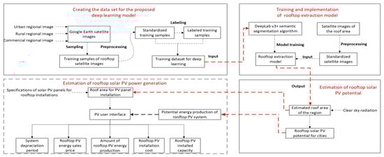
Figure 1.
Research flow chart.
2.1. Overall Research Framework
The research framework in this study consists of four main modules: creating the dataset with pixel-wise manual labeling, training and testing the network for rooftop area estimation, determining the rooftop PV generation potential on a city basis, and designing a PV user interface to evaluate the PV generation results.
The resulting model was subjected to validation and evaluation phases on test images taken from different regions, and its performance was analyzed using the IoU metric. The model was found to accurately distinguish roof regions with high accuracy rates. Accordingly, potential rooftop PV areas were calculated on a city-by-city basis using the estimated rooftop zones, and a comprehensive PV generation potential analysis was conducted for 81 provinces of Turkey.
In addition, a user interface was designed to enable users to evaluate the model results in a practical way. Through this interface, users can automatically identify rooftop areas in the satellite images they upload and calculate basic parameters such as PV installed capacity, annual energy production, investment cost, energy sales revenue, and system amortization period according to the selected city and panel type.
2.2. Satellite Images for Dataset Preparation
2.2.1. Urban, Rural, and Industrial Area Satellite Image Acquisition
In this study, the AIRS platform [53], which provides publicly available aerial imagery, was used as the data source. A dataset of 100 images covering an area of approximately 45.7 km2 was used for the analysis. All downloaded images have high spatial resolution. These 10,000 × 10,000-pixel images clearly visualize the architectural details of a building. In order to obtain stable and consistent results in deep learning network training, 100 images were selected from rural, urban, and industrial regions. The majority of the roofs in the images were obtained from buildings with a low number of stories. The roofs in the selected regions were considered horizontal in shape.
2.2.2. Sample Labeling
In the deep learning method used in this study, labeled images corresponding to remote sensing images need to be produced in order to train and test the model. Remote sensing images were manually labeled on a pixel basis, and the MATLAB R2023a Image Segmenter tool was used for this process. During the labeling phase, obstacles on the roof were not included in the labeling process. Furthermore, shadowy areas on the roof caused by vegetation and clouds were not included in the labeled pixels. Sample images of the labeling process are presented in Figure 2.
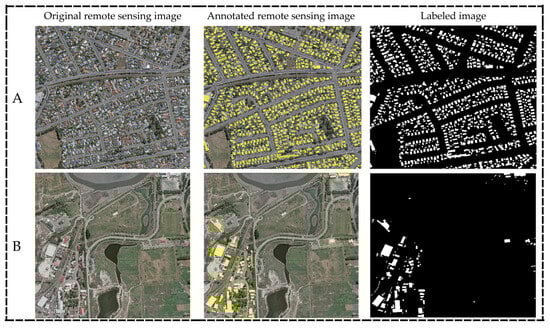
Figure 2.
Example of labeled image production results. (A) Labeled image production results for urban area; (B) Labeled image production for industrial area.
For the training of the deep learning network, over 20,000 roof regions were manually labeled at the pixel level and made suitable for the training process. Since the dataset contains a sufficient number of remote sensing images and a sufficient variety of roof regions within these images, data augmentation methods were not required. The pixel-based manual labeling approach resulted in high accuracy and quality roof labels. The training dataset created in this study consists of remote sensing images and the corresponding labeled images. The remote sensing images used in the sample are 10,000 × 10,000 pixels in size, and the corresponding labeled images are 1536 × 1536 pixels in resolution. Before the training process, all images were resized to 512 × 512 pixels to make them suitable for model training.
2.3. Training and Implementation of the Roof Zone Identification Model
2.3.1. Roof Region Extraction Algorithm
In this study, roof regions are extracted using an image semantic segmentation algorithm based on different variations of DeepLabv3+. Different variations of the U-Net and DeepLabv3+ deep learning architectures were tested in the training stages of the model, and the results showed that the DeepLabv3+ architecture performed better. DeepLabv3+ [54] effectively captures multi-scale contextual information through its modified and extended convolutional structure. DeepLabv3+ includes an Atrous Spatial Pyramid Pooling (ASPP) module to enhance the multi-scale feature representation, thereby producing accurate segmentation results. The model used in this study includes the ResNet50 backbone network in the encoder part, followed by multiple convolutional layers to capture the complex spatial context. The ResNet50 backbone network was chosen due to its advantages, such as lower GPU requirements, its use in real-time systems (e.g., user interface-based applications), and lower risk of over-learning. The Resnet101 network may be preferred for studies with larger datasets and higher GPU requirements.
In the decoder part, bilinear up-sampling is used to achieve accurate segmentation. After all remote sensing images are extracted and manually labeled, the roof regions are used as input data for the DeepLabv3+ algorithm to train the semantic segmentation model. The basic architecture of DeepLabv3+ is presented in Figure 3.
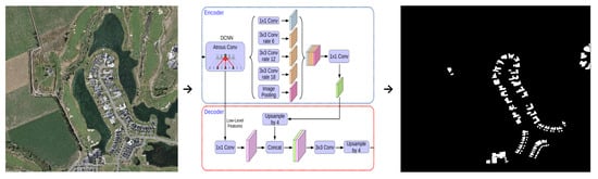
Figure 3.
Using DeepLabv3+ deep learning approach for roof segmentation.
The input image of the network model to be trained is shown in Equation (1). Here, represents the input image:
The second step is the feature extraction layer. In this stage, high-level feature maps are extracted from the image using deep neural network architectures (usually ResNet-101 or ResNet-50). The mathematical expression of this process is presented in Equation (2).
In this step, denotes the feature map obtained from the backbone network. The third step involves the convolution layers. In particular, the mathematical expression for the Atrous (extended) convolution layer is presented in Equation (3).
In this expression, represents the input image, represents the filter weights, represents the dilation ratio, and represents the output image. In the fourth step, ASPP is performed. In this step, multiple convolution layers with different dilation ratios are used in parallel to collect contextual information from small, medium, and large objects. The mathematical expression for this layer is presented in Equation (4).
The ⨁ operator refers to the consolidation of the outputs from multiple Atrous convolution layers. In the consolidation stage, the feature maps from the ASPP are combined and then dimensionally reduced by a convolution process. In this stage, normalization and activation functions are also applied. The mathematical expression for these operations is presented in Equation (5).
In the next step, upsampling is performed. In this step, the resulting output segmentation map is scaled to the original image size. Generally, bilinear interpolation is used in this process. The mathematical expression for this step is presented in Equation (6).
One of the last steps, the prediction phase, predicts which class each pixel belongs to. By applying the softmax function, the class probabilities are obtained for each pixel. The mathematical expression of the prediction expression is given in Equation (7), and the mathematical expression of the loss function is given in Equation (8).
is the true label, is the prediction output, is the number of pixels, and is the number of classes.
2.3.2. Roof Zone Extraction Training
When training deep learning networks, the input image size was set to 512 × 512 pixels and 2 channels in order to increase training efficiency and optimize video memory usage considering the physical limitations of computer memory and graphics processing unit (GPU) memory. In order to improve the inference performance of the model and to optimize the training algorithm, the gradient descent-based Adam (Adaptive Moment Estimation) optimization method was used. This method adaptively adjusts the learning rate for each parameter and optimizes the weight updates by considering the first and second moment estimates of the gradients. In the training process of the model, the number of classes was set to 2, the test dataset weight was increased, the number of layers in the network was reduced, and the risk of overfitting was reduced by shuffling the dataset at the end of each epoch. Optimal accuracy and loss values were achieved by using a mini-batch size of 4 images at each step. Table 2 summarizes the main parameters used in model training.
Table 2.
Training parameters for deep learning models.
After manually labeling the roof samples of the study area, the training dataset was provided as input data to the U-Net and DeepLabv3+ models. In order to improve the prediction accuracy of the model, four different variations of the U-Net and DeepLabv3+ architectures were evaluated, and independent training processes were performed for each of them. These variations were modeled using different backbone architectures, hyperparameter settings, and training strategies. The performance indicators obtained for each model variation are summarized in Table 3.
Table 3.
Training performance results for deep learning models.
2.3.3. Roof Region Extraction Model Implementation
The dataset was given as input to the DeepLabv3+ architecture, and a model with ideal performance for roof region extraction was obtained. A large number of satellite images from different regions were applied to the model, and roof regions in these images were successfully detected. Since the image dimensions used in the training process are 512 × 512 pixels, the input images should have the same dimensions in the prediction phase. The roof region extraction accuracy of the model was tested by directly resizing the high-resolution input images instead of processing them into smaller blocks. The model trained with this block-based estimation method was successfully applied to satellite images with different resolutions, and as a result, roof region segmentation outputs were obtained.
2.3.4. Roof Extraction Model Performance Evaluation
After successfully extracting roof regions at the scale of urban, rural, and industrial areas using the DeepLabv3+ model, it became necessary to validate the roof extraction performance of the model. The IoU metric was used to evaluate the area extraction performance of the model trained with a pixel-based segmentation approach. IoU is a basic validation criterion that measures the overlap between the roof pixels predicted by the model and the actual roof pixels for a roof region.
2.4. Rooftop Solar PV Potential Estimation Model
In this study, the roof of a building is considered as a horizontal plane. The total amount of radiation is the sum of direct and indirect solar radiation. The performance of a solar power generation system depends on parameters such as solar radiation and atmospheric temperature. The output power generated by the PV array is given in Equation (9).
is the power output of the PV array, is the number of modules, is the open-circuit voltage, is the short-circuit current, is the fill factor, is the open-circuit voltage under STC, and is the short-circuit current under STC. Short-circuit current is calculated using Equation (10), short-circuit voltage using Equation (11), and cell temperature using Equation (12).
(0.0005 A/°C) is the short-circuit current temperature coefficient, (−0.003 V/°C) is the open-circuit voltage temperature, is the cell temperature, is the nominal cell operating temperature (43 °C), (25 °C) is the ambient temperature, and (150–250 w/) is the instantaneous radiation amount.
Solar radiation data were used to determine the amount of energy to be generated from solar power plants (SPPs) with a certain installed capacity. There are some parameters that determine the amount of solar energy production. One of them is the amount of radiation. The value at which solar radiation creates current on the panels is calculated in Equation (13).
is the maximum radiation amount (1000 w) falling on the panel, is the current value produced by the PV panel under maximum radiation conditions, and is the panel output current produced under the radiation amount at instant . In line with these basic parameters, the amount of energy that a solar energy system with a power of 1 kWp can produce on average in a year for 81 provinces of Turkey was calculated to be presented to the users in the PV user interface. The results are presented in Figure 4.
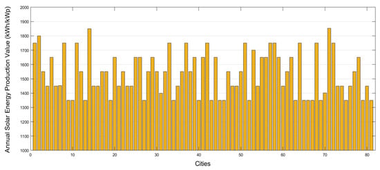
Figure 4.
For 81 cities, the average annual energy production amount in a system with 1 kWp installed power.
In the next step, PV system installed power values for different roof regions were calculated using Equation (14).
stands for the installed capacity of the PV system, stands for the estimated total roof area, and stands for the panel efficiency ratio. Three different panel types are considered in the analysis: monocrystalline, polycrystalline, and thin film. The annual energy production amount of rooftop PV systems is calculated using Equation (15), the system installation cost is calculated using Equation (16), the annual energy sales revenue is calculated using Equation (17), and the system amortization period is calculated using Equation (18).
In this study, is the yearly energy produced by solar panels on the roof, is the average yearly energy output of a solar power plant with a capacity of 1 kWp, is the price for each square meter of the panel, is the yearly income from selling energy, and SAP is how long the system lasts before it loses value.
The main input data used in PV potential estimation consist of the roof surface area calculated from the forecast images, the annual generation capacity of a 1-kilowatt peak power SPP on a city basis, and the efficiency ratios determined according to the selected panel type (monocrystalline, polycrystalline, and thin film).
It is known that as the area of PV installation increases, the share of installation costs other than panel costs per unit area decreases. Non-panel cost items are classified as inverter, installation and assembly operations, electrical equipment, labor, and engineering expenses. Accordingly, in order to calculate the total installation cost more accurately, rooftop areas were categorized as low-, medium-, and high-density areas, and different cost multipliers were determined for each density level.
3. Results and Discussion
In the second section, the processes of sample collection, sample processing, rooftop region extraction, area estimation, and PV generation estimation are presented in detail. In this section, the results obtained to evaluate the performance of the proposed methodology for both rooftop PV area potential and rooftop solar PV power generation are described.
3.1. Roof Region Extraction Results
As a result of the area extraction for 100 different roof regions, the total estimated roof area was calculated as 2.76 km2. Sample results for the performance evaluation of the model developed after roof area extraction were determined for three different roof areas, and these results are presented in Figure 5.
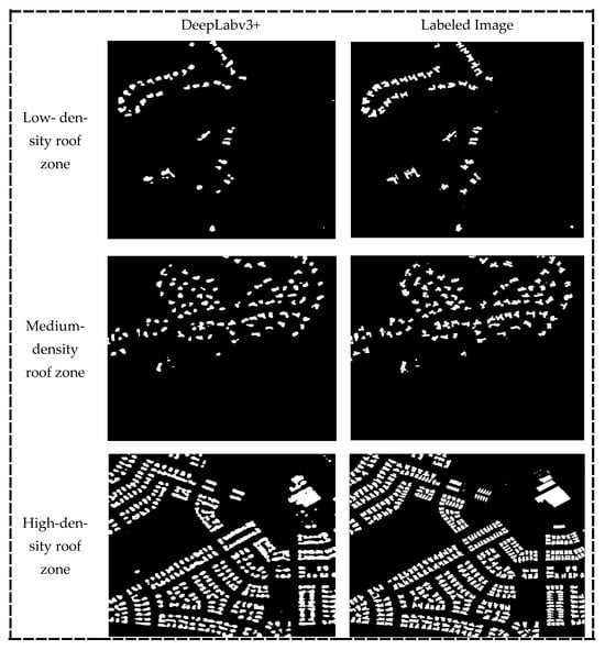
Figure 5.
Analysis of predicted roof area and actual roof area.
The satellite images used for performance evaluation were selected from urban, rural, and industrial areas. When the area estimation and IoU performance results of the model are analyzed, optimal results are obtained in terms of roof area extraction and area estimation. The first example presented in Figure 5 is selected from a low-density rural roof region, and the IoU rate for this image with a total roof area of 15,730 m2 is calculated as 78.18%. The second sample is taken from an urban medium-density roof area, and the IoU ratio is 80.16% for a total roof area of 41,185 m2. The last sample was selected from an urban high-density rooftop zone, and the IoU ratio was recorded as 82.6% for a total roof area of 274,163 m2.
The PV area estimates are based on un-orthorectified satellite imagery. This resulted in limited spatial shifts between the estimated roof areas and the actual roof locations. Although the effect of positional shifts is more pronounced in high-rise buildings, it is negligible in low-rise buildings. Furthermore, these spatial shifts do not significantly affect the total roof area calculations for rooftop PV potential estimates at the city scale.
In this stage, the area calculations and image-based IoU ratios were tested on 100 different roof regions to evaluate the overall performance of the trained model. For 100 roof regions, the predicted roof segmentation results are compared with the actual labeled images, and the IoU results are presented in Figure 6.
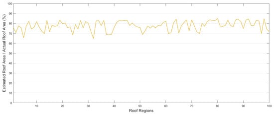
Figure 6.
IoU success rates for 100 roof regions.
The 100 different roof regions analyzed were selected from urban, rural, and industrial satellite images. When the IoU results are analyzed, the highest accuracy rate is 84.84%, and the lowest accuracy rate is 64.80%. The model successfully detected roof regions and calculated the related areas with an average accuracy of 77.11% across these 100 regions.
The roof area estimates obtained do not include structural information such as the slope, height, and detailed form of the roof. It is very difficult to accurately extract the geometric features of the roof (e.g., angle of inclination, height, and complex forms) based on satellite imagery. Such detailed structural information of the roof often requires high-precision 3D roof models for city-scale analysis. Future work plans to integrate methods for reconstructing the geometric structure of the roof using open street view images [55].
With the dataset prepared in this study, semantic segmentation training was performed using DeepLabv3+ architecture. Although the training process is time consuming and technically complex, limiting the number of classes to only two categories, “roof” and “background,” and performing the labeling process on a pixel basis enabled the model to achieve optimal results in both training and prediction phases.
When the DeepLabv3+ model trained using the Adam algorithm was evaluated in terms of roof region extraction performance in satellite images of different region types, it produced successful results in urban, rural, and industrial regions. Since the roof areas in rural areas are generally smaller and irregular, the prediction accuracy of the model in these areas was relatively lower. In addition, the diversity and irregularity of building types in rural areas increased the prediction difficulty of the model and created a strong randomness and subjectivity in the training process.
3.2. Estimation and Temporal Analysis of Rooftop Solar PV Potential
3.2.1. Estimation of Rooftop Solar PV Energy Production
Accurate estimation of rooftop solar energy potential is critical for determining the installed capacity of rooftop PV systems. In order to achieve maximum electricity generation from rooftop PV systems, the nominal power of PV panels should be selected in accordance with the solar radiation per unit area of rooftops in the region.
In this study, the total PV energy that can be generated on an annual basis for 81 provinces of Turkey is calculated. The cost per square meter of PV panels varies according to the panel type and is determined as 3000 TL/m2 for monocrystalline panels, 2500 TL/m2 for polycrystalline panels, and 2000 TL/m2 for thin-film panels. Panel prices are based on the average PV panel costs of solar power plants located in different regions in Turkey. This cost scale is valid for 2025. Total PV system installation costs are calculated according to the area density multipliers given in Table 4.
Table 4.
PV system installation costs according to roof area densities.
While determining the multipliers for total cost, inverter, installation, and assembly operations, electrical equipment, labor, and engineering expenses other than panel costs are taken as the basis. The installed power of a roof-mounted PV system is calculated by multiplying the automatic roof surface area extracted by deep learning-based roof area estimation and the efficiency ratio of the selected panel type. The annual energy production potential of the relevant roof area is obtained by multiplying the calculated installed capacity by the average annual energy production value per 1 kWp for that city.
Within the scope of this study, the total size of roof areas suitable for PV panel installation was estimated to be approximately 2.78 km2 using the trained model. Considering the average panel efficiency rates and the average annual solar energy production values for 81 provinces of Turkey, the average annual energy production potential for a city is calculated as approximately 10.02 GWh.
3.2.2. Rooftop Solar PV Potential Estimation Results
In this study, a user interface was developed that can make regional roof forecasts by calculating the insolation values of 81 provinces, perform area calculations from the estimated roof areas, and calculate all the outputs required for rooftop PV applications according to the city and panel type information selected by the user. This interface was designed and created in the Matlab GUI platform. This platform, which is unique in itself, has a function that can be applied not only in Turkey but also in any region. A visualization of this interface is presented in Figure 7.
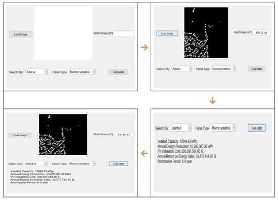
Figure 7.
PV cooperative user interface.
When an image is uploaded to the user interface by an individual energy user, the roof regions in this image are automatically detected in the background by the trained deep learning model, and the results are presented to the user in binary image format. At the same time, the total area value corresponding to the detected roof regions (white areas) is also displayed on the screen.
In the next step, when the user selects the city and the preferred panel type and presses the calculation button, the system automatically calculates and presents the basic performance parameters, such as PV installed capacity, annual PV energy production, PV installation cost, annual energy sales revenue, and system amortization period, for the total estimated roof area. According to the results obtained, the amortization period is calculated as the shortest, with an average of 4.5 years in the case of polycrystalline panels in high-density roof areas. The highest amortization period in the same region was recorded as 6.2 years. For monocrystalline panel selection, the amortization period ranged between 4.9 years and 6.7 years in high-density regions, while for thin-film panels, this period was measured between 5.6 years and 7.8 years. The amortization period calculations for high-density roof regions based on 81 provinces are shown in Figure 8.
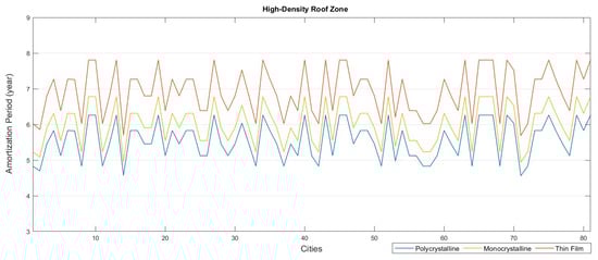
Figure 8.
Amortization period by panel types for cities with high roof density.
In the case of polycrystalline panels in medium-density roof areas, amortization periods were calculated between 5.8 and 8 years. For monocrystalline panels, these periods ranged between 6.1 and 8.5 years, and for thin-film panels, between 7.1 and 9.7 years. In low-density roof areas, amortization periods were calculated to be longer. When polycrystalline panels are used, amortization periods vary between 7.8 and 10.7 years, changing to 8.2 and 11.3 years for monocrystalline panels and 9.4 and 13 years for thin-film panels. The regions entered in the user interface are open to universality. The roof forecast image can be extracted with images taken not only from Turkey but also from any region in the world. Afterwards, PV system depreciation times can be obtained by defining the insolation values of that region to the interface.
These values are based on the interface developed for rooftop PV users, enabling highly accurate rooftop area extraction and automated detailed solar energy production and cost calculations depending on the selected city and panel type. In future research, different data sources and model configurations will be used to improve the accuracy of prediction and refine the area calculations. The calculation results for rooftop solar power generation represent theoretical design values only and do not fully reflect the energy production to be achieved in actual field installations.
Although extensive city-scale analyses have been performed, it is important for consistency to use images of low-density rooftop areas in the estimation process, as energy cooperatives operate in smaller areas. Different coefficients used in the user interface for low-, medium-, and high-density regions allow for more realistic and region-specific cost analysis. The transition from fossil fuels to renewable energy is vital to achieve the key goal of the Paris Agreement and to build a sustainable energy system for the future. The deployment of solar PVs will play a key role in the energy transition of countries. A clear and consistent analysis of PV potential will help local governments to promote future decarbonization. According to our study results, tests and estimations were performed on a roof area of 2.78 km2. To evaluate the model’s predictive performance, images containing rooftops were selected from urban, rural, and commercial areas. Furthermore, these images were selected to equally represent low, medium, and high roof densities to improve the model’s overall consistency. The expansion of energy cooperative networks in cities will accelerate the promotion and viability of rooftop PV installations.
In future work, we aim to explore roof geometry reconstruction methods based on publicly available high-resolution remote sensing image data. We also aim to analyze the impact of different architectural styles in cities on solar energy potential. Finally, considering that rooftop areas in regional energy cooperatives are generally of limited size, we aim to conduct detailed rooftop identification, technical feasibility, and economic analysis for small-scale rooftop areas in the future. The impact of building distribution on solar energy potential is mainly related to the storage and transmission of generated solar energy to the grid. Scientific planning of the location and capacity of distributed solar PV systems is of great importance. Connecting a large distributed solar PV system to the distribution grid has significant impacts in terms of voltage level, grid loss, and reliability. The size of this impact is closely related to the installation location and capacity of the distributed solar PV system.
4. Conclusions
In this study, a holistic method is proposed to estimate rooftop solar PV potential at the city scale using publicly available satellite imagery and to perform detailed PV calculations through a user interface. The proposed method is based on prior knowledge and comprehensive datasets for urban, rural, and industrial regions and provides an easily applicable structure for large-scale rooftop solar PV potential estimation. The prepared dataset was tested using U-Net and DeepLabv3+ segmentation models, and the results showed that the DeepLabv3+ model performed better during training. Existing rooftop regions are successfully extracted from remote sensing images using the DeepLabv3+ semantic segmentation model. Through the user interface, the PV potential and rooftop PV energy production for the estimated rooftop regions are automatically calculated based on the extracted area values.
Urban, rural, and industrial rooftops were identified from large satellite imagery with an average accuracy of 98%. In a total estimated roof area of 2.78 , an average IoU success rate of 77.11% was achieved for 100 different roof regions. In these regions, the highest roof prediction accuracy was 84.84%, and the lowest accuracy was 64.8%. Based on the rooftop PV generation model, the average annual energy production for a rooftop zone is calculated as 10.02 GWh. The developed model is able to estimate rooftop zones without requiring a 3D building model, which shows that the model has high flexibility and allows for fast and practical rooftop solar PV potential assessments in large-scale areas.
Deep learning-based image semantic segmentation technology significantly improves image segmentation accuracy. Especially comprehensive datasets labeled at the pixel level are vital to the success of these technologies. In the future, more advanced semantic segmentation models will be used to further improve the performance of the roof extraction model. In this study, building roofs are analyzed as a horizontal plane. Moreover, in order to improve the training and prediction accuracy of the model, the dataset was refined, and the number of classes was simplified to only “roof” and “background.” Thanks to the developed user interface, energy users who will install rooftop PVs can easily view the most suitable installation options and estimated amortization periods through the roof regions predicted with high accuracy.
According to the results, the amortization period of PV systems ranges from 4.5 to 7.8 years in high-density roof regions, 5.8 to 9.75 years in medium-density roof regions, and 7.8 to 13 years in low-density roof regions. This shows that roof density has a significant impact on the PV system payback period.
Author Contributions
Conceptualization, A.H.; methodology, A.H.; writing—original draft, A.H.; writing—review and editing, A.E. and A.K. All authors have read and agreed to the published version of the manuscript.
Funding
This research received no external funding.
Institutional Review Board Statement
Not applicable.
Informed Consent Statement
Not applicable.
Data Availability Statement
The original contributions presented in this study are included in the article. Further inquiries can be directed to the corresponding author.
Conflicts of Interest
The authors declare no conflicts of interest.
Abbreviations
The following abbreviations are used in this manuscript:
| PV | Photovoltaic |
| IoU | Intersection over union |
| LIDAR | Light detection and ranging |
| DSM | Digital surface modeling |
| ASPP | Atrous spatial pyramid pooling |
| CNN | Convolutional neural network |
| GPU | Graphic processing unit |
| kWp | Kilowatt peak |
| kWh | Kilowatt hour |
| GWh | Gigawatt hour |
| PSIP | Power system installed capacity |
| ERA | Estimated roof area |
| PER | Panel efficiency ratio |
| PSIC | Photovoltaic system installation cost |
| APPQ | Annual PV production quantity |
| AAEP | Average annual energy production |
| ESP | Energy sales price |
| SAP | System amortized period |
| AESR | Annual energy sales revenue |
References
- Duan, H.B.; Zhang, G.P.; Zhu, L.; Fan, Y.; Wang, S.Y. How will diffusion of PV solar contribute to China’s emissions-peaking and climate responses? Renew. Sustain. Energy Rev. 2016, 53, 1076–1085. [Google Scholar] [CrossRef]
- Tyagi, V.V.; Rahim, N.A.; Rahim, N.A.; Jeyraj, A.; Selvaraj, L. Progress in solar PV technology: Research and achievement. Renew. Sustain. Energy Rev. 2013, 20, 443–461. [Google Scholar] [CrossRef]
- Lan, H.; Gou, Z.; Xie, X. A simplified evaluation method of rooftop solar energy potential based on image semantic segmentation of urban streetscapes. Sol. Energy 2021, 230, 912–924. [Google Scholar] [CrossRef]
- IEA. Global Solar PV Market Set for Spectacular Growth over Next 5 Years. Available online: https://www.iea.org/news/global-solar-pv-market-set-for-spectacular-growth-over-next-5-years (accessed on 16 June 2022).
- IRENA. Renewable Power Generation Costs in 2022. Available online: https://www.irena.org/Publications/2023/Aug/Renewable-Power-Generation-Costs-in-2022 (accessed on 15 February 2024).
- Sun, T.; Shan, M.; Rong, X.; Yang, X. Estimating the spatial distribution of solar photovoltaic power generation potential on different types of rural rooftops using a deep learning network applied to satellite images. Appl. Energy 2022, 315, 119025. [Google Scholar] [CrossRef]
- NREL. Best Research-Cell Efficiency Chart|Photovoltaic Research. Available online: https://www.nrel.gov/pv/cell-efficiency.html (accessed on 15 February 2024).
- Hamzaoğlu, A.; Erduman, A.; Alçı, M. Reduction of distribution system losses using solar energy cooperativity by home user. Ain Shams Eng. J. 2021, 12, 3737–3745. [Google Scholar] [CrossRef]
- Assouline, D.; Mohajeri, N.; Scartezzini, J.L. Quantifying rooftop photovoltaic solar energy potential: A machine learning approach. Sol. Energy 2017, 141, 278–296. [Google Scholar] [CrossRef]
- Liang, J.; Gong, J.; Li, W. Applications and impacts of Google Earth: A decadal review (2006–2016). ISPRS J. Photogramm. Remote Sens. 2018, 146, 91–107. [Google Scholar] [CrossRef]
- Qi, F.; Wang, Y. A new calculation method for shape coefficient of residential building using Google Earth. Energy Build. 2014, 76, 72–80. [Google Scholar] [CrossRef]
- Liu, X.; Deng, Z.; Yang, Y. Recent progress in semantic image segmentation. Artif. Intell. Rev. 2019, 52, 1089–1106. [Google Scholar] [CrossRef]
- Ravishankar, R.; AlMahmoud, E.; Habib, A.; de Weck, O.L. Capacity estimation of solar farms using deep learning on high-resolution satellite imagery. Remote Sens. 2022, 15, 210. [Google Scholar] [CrossRef]
- Jiang, H.; Yao, L.; Lu, N.; Qin, J.; Liu, T.; Liu, Y.; Zhou, C. Multi-resolution dataset for photovoltaic panel segmentation from satellite and aerial imagery. Earth Syst. Sci. Data Discuss. 2021, 2021, 1–17. [Google Scholar] [CrossRef]
- Zhu, R.; Guo, D.; Wong, M.S.; Qian, Z.; Chen, M.; Yang, B.; Chen, B.; Zhang, H.; You, L.; Yan, J.; et al. Deep solar PV refiner: A detail-oriented deep learning network for refined segmentation of photovoltaic areas from satellite imagery. Int. J. Appl. Earth Obs. Geoinf. 2023, 116, 103134. [Google Scholar] [CrossRef]
- Kleebauer, M.; Marz, C.; Reudenbach, C.; Braun, M. Multi-resolution segmentation of solar photovoltaic systems using deep learning. Remote Sens. 2023, 15, 5687. [Google Scholar] [CrossRef]
- Shi, Y.; Li, Q.; Zhu, X.X. Building segmentation through a gated graph convolutional neural network with deep structured feature embedding. ISPRS J. Photogramm. Remote Sens. 2020, 159, 184–197. [Google Scholar] [CrossRef] [PubMed]
- Cabras, M.; Pilloni, V.; Atzori, L. A novel smart home energy management system: Cooperative neighbourhood and adaptive renewable energy usage. In Proceedings of the 2015 IEEE International Conference on Communications (ICC), London, UK, 8–12 June 2015; pp. 716–721. [Google Scholar] [CrossRef]
- Ouammi, A. Optimal power scheduling for a cooperative network of smart residential buildings. IEEE Trans. Sustain. Energy 2016, 7, 1317–1326. [Google Scholar] [CrossRef]
- Mignon, I.; Rüdinger, A. The impact of systemic factors on the deployment of cooperative projects within renewable electricity production–An international comparison. Renew. Sustain. Energy Rev. 2016, 65, 478–488. [Google Scholar] [CrossRef]
- Wirth, S. Communities matter: Institutional preconditions for community renewable energy. Energy Policy 2014, 70, 236–246. [Google Scholar] [CrossRef]
- Nasrallah, H.; Samhat, A.E.; Shi, Y.; Zhu, X.X.; Faour, G.; Ghandour, A.J. Lebanon solar rooftop potential assessment using buildings segmentation from aerial images. IEEE J. Sel. Top. Appl. Earth Obs. Remote Sens. 2022, 15, 4909–4918. [Google Scholar] [CrossRef]
- Sampath, A.; Bijapur, P.; Karanam, A.; Umadevi, V.; Parathodiyil, M. Estimation of rooftop solar energy generation using satellite image segmentation. In Proceedings of the 2019 IEEE 9th International Conference on Advanced Computing (IACC), Tiruchirappalli, India, 13–14 December 2019; pp. 38–44. [Google Scholar] [CrossRef]
- Zhong, T.; Zhang, Z.; Chen, M.; Zhang, K.; Zhou, Z.; Zhu, R.; Wang, Y.; Lü, G.; Yan, J. A city-scale estimation of rooftop solar photovoltaic potential based on deep learning. Appl. Energy 2021, 298, 117132. [Google Scholar] [CrossRef]
- Ni, H.; Wang, D.; Zhao, W.; Jiang, W.; Mingze, E.; Huang, C.; Yao, J. Enhancing rooftop solar energy potential evaluation in high-density cities: A Deep Learning and GIS based approach. Energy Build. 2024, 309, 113743. [Google Scholar] [CrossRef]
- Chen, B.; Che, Y.; Wang, J.; Li, H.; Yu, L.; Wang, D. An estimation framework of regional rooftop photovoltaic potential based on satellite remote sensing images. Glob. Energy Interconnect. 2022, 5, 281–292. [Google Scholar] [CrossRef]
- Lodhi, M.K.; Tan, Y.; Wang, X.; Masum, S.M.; Nouman, K.M.; Ullah, N. Harnessing rooftop solar photovoltaic potential in Islamabad, Pakistan: A remote sensing and deep learning approach. Energy 2024, 304, 132256. [Google Scholar] [CrossRef]
- Li, G.; Wang, Z.; Xu, C.; Li, T.; Gao, J.; Mao, Q.; Chen, S. A district-scale spatial distribution evaluation method of rooftop solar energy potential based on deep learning. Sol. Energy 2024, 268, 112282. [Google Scholar] [CrossRef]
- Ren, H.; Sun, Y.; Zhang, Y. A novel 3D-geographic information system and deep learning integrated approach for high-accuracy building rooftop solar energy potential characterization of high-density cities. In Building Simulation 2023; IBPSA: Las Cruces, NM, USA, 2023; Volume 18, pp. 1299–1306. [Google Scholar] [CrossRef]
- Kalyan, S.; Sun, Q. Interrogating the installation gap and potential of solar photovoltaic systems using GIS and deep learning. Energies 2022, 15, 3740. [Google Scholar] [CrossRef]
- Yang, J.; Matsushita, B.; Zhang, H. Improving building rooftop segmentation accuracy through the optimization of UNet basic elements and image foreground-background balance. ISPRS J. Photogramm. Remote Sens. 2023, 201, 123–137. [Google Scholar] [CrossRef]
- Frimane, Â.; Johansson, R.; Munkhammar, J.; Lingfors, D.; Lindahl, J. Identifying small decentralized solar systems in aerial images using deep learning. Sol. Energy 2023, 262, 111822. [Google Scholar] [CrossRef]
- Jiang, H.; Yao, L.; Lu, N.; Qin, J.; Liu, T.; Liu, Y.; Zhou, C. Geospatial assessment of rooftop solar photovoltaic potential using multi-source remote sensing data. Energy AI 2022, 10, 100185. [Google Scholar] [CrossRef]
- García, G.; Aparcedo, A.; Nayak, G.K.; Ahmed, T.; Shah, M.; Li, M. Generalized deep learning model for photovoltaic module segmentation from satellite and aerial imagery. Sol. Energy 2024, 274, 112539. [Google Scholar] [CrossRef]
- Mao, H.; Chen, X.; Luo, Y.; Deng, J.; Tian, Z.; Yu, J.; Xiao, Y.; Fan, J. Advances and prospects on estimating solar photovoltaic installation capacity and potential based on satellite and aerial images. Renew. Sustain. Energy Rev. 2023, 179, 113276. [Google Scholar] [CrossRef]
- Mainzer, K.; Killinger, S.; McKenna, R.; Fichtner, W. Assessment of rooftop photovoltaic potentials at the urban level using publicly available geodata and image recognition techniques. Sol. Energy 2017, 155, 561–573. [Google Scholar] [CrossRef]
- Liu, J.; Wu, Q.; Lin, Z.; Shi, H.; Wen, S.; Wu, Q.; Zhang, J.; Peng, C. A novel approach for assessing rooftop-andfacade solar photovoltaic potential in rural areas using three-dimensional (3D) building models constructed with GIS. Energy 2023, 282, 128920. [Google Scholar] [CrossRef]
- Guo, Z.; Zhuang, Z.; Tan, H.; Liu, Z.; Li, P.; Lin, Z.; Shang, W.-L.; Zhang, H.; Yan, J. Accurate and generalizable photovoltaic panel segmentation using deep learning for imbalanced datasets. Renew. Energy 2023, 219, 119471. [Google Scholar] [CrossRef]
- Jurakuziev, D.; Jumaboev, S.; Lee, M. A framework to estimate generating capacities of PV systems using satellite imagery segmentation. Eng. Appl. Artif. Intell. 2023, 123, 106186. [Google Scholar] [CrossRef]
- Yan, L.; Zhu, R.; Kwan, M.P.; Luo, W.; Wang, D.; Zhang, S.; Wong, M.S.; You, L.; Yang, B.; Feng, L.; et al. Estimation of urban-scale photovoltaic potential: A deep learning-based approach for constructing three-dimensional building models from optical remote sensing imagery. Sustain. Cities Soc. 2023, 93, 104515. [Google Scholar] [CrossRef]
- Yang, R.; He, G.; Yin, R.; Wang, G.; Zhang, Z.; Long, T.; Peng, Y. Weakly-semi supervised extraction of rooftop photovoltaics from high-resolution images based on segment anything model and class activation map. Appl. Energy 2024, 361, 122964. [Google Scholar] [CrossRef]
- Pueblas, R.; Kuckertz, P.; Weinand, J.M.; Kotzur, L.; Stolten, D. ETHOS. PASSION: An open-source workflow for rooftop photovoltaic potential assessments from satellite imagery. Sol. Energy 2023, 265, 112094. [Google Scholar] [CrossRef]
- Amo-Boateng, M.; Sey, N.E.N.; Amproche, A.A.; Domfeh, M.K. Instance segmentation scheme for roofs in rural areas based on Mask R-CNN. Egypt. J. Remote Sens. Space Sci. 2022, 25, 569–577. [Google Scholar] [CrossRef]
- Tao, L.; Hayashi, K.; Shiraki, H.; Huang, X.; Dem, P. Exploration of determinants underlying regional disparity in rooftop photovoltaic adoption: A case study in Nagoya, Japan. Appl. Energy 2024, 367, 123469. [Google Scholar] [CrossRef]
- Tian, J.; Ooka, R.; Lee, D. Multi-scale solar radiation and photovoltaic power forecasting with machine learning algorithms in urban environment: A state-of-the-art review. J. Clean. Prod. 2023, 426, 139040. [Google Scholar] [CrossRef]
- Casini, M.; De Angelis, P.; Chiavazzo, E.; Bergamasco, L. Current trends on the use of deep learning methods for image analysis in energy applications. Energy AI 2024, 15, 100330. [Google Scholar] [CrossRef]
- Tan, H.; Guo, Z.; Zhang, H.; Chen, Q.; Lin, Z.; Chen, Y.; Yan, J. Enhancing PV panel segmentation in remote sensing images with constraint refinement modules. Appl. Energy 2023, 350, 121757. [Google Scholar] [CrossRef]
- Li, Z.; Zhang, C.; Yu, Z.; Zhang, H.; Jiang, H. Deep Learning Method for Evaluating Photovoltaic Potential of Rural Land Use Types. Sustainability 2023, 15, 10798. [Google Scholar] [CrossRef]
- Zhang, Y.; Han, F.; Zhou, M.; Hou, Y.; Wang, S. Application of Deep Learning in Glacier Boundary Extraction: A Case Study of the Tomur Peak Region, Tianshan, Xinjiang. Sustainability 2025, 17, 3678. [Google Scholar] [CrossRef]
- Kumar, R.; Saha, R.; Simic, V.; Dev, N.; Kumar, R.; Banga, H.K.; Bacanin, N.; Singh, S. Rooftop solar potential in micro, small, and medium size enterprises: An insight into renewable energy tapping by decision-making approach. Sol. Energy 2024, 276, 112692. [Google Scholar] [CrossRef]
- Ferry, A.; Thebault, M.; Nérot, B.; Berrah, L.; Ménézo, C. Modeling and analysis of rooftop solar potential in highland and lowland territories: Impact of mountainous topography. Sol. Energy 2024, 275, 112632. [Google Scholar] [CrossRef]
- Xu, X.; Hu, J.; Zhang, H.; Feng, Y.; Yang, J.; Tan, Z.; Bai, J. Photovoltaic resource assessment through roof usable area extraction based on image segmentation. Sol. Energy 2025, 297, 113646. [Google Scholar] [CrossRef]
- Atilol. Aerial Imagery for Roof Segmentation. [Data Set]. Kaggle. Available online: https://www.kaggle.com/datasets/atilol/aerialimageryforroofsegmentation (accessed on 10 July 2024).
- Chen, L.C.; Zhu, Y.; Papandreou, G.; Schroff, F.; Adam, H. Encoder-decoder with atrous separable convolution for semantic image segmentation. In Proceedings of the European Conference on Computer Vision (ECCV), Munich, Germany, 8–14 September 2018; pp. 801–818. [Google Scholar] [CrossRef]
- Zamir, A.R.; Wekel, T.; Agrawal, P.; Wei, C.; Malik, J.; Savarese, S. Generic 3d representation via pose estimation and matching. In Proceedings of the Computer Vision–ECCV 2016: 14th European Conference, Amsterdam, The Netherlands, 11–14 October 2016; Proceedings, Part III 14. Springer International Publishing: Berlin/Heidelberg, Germany, 2016; pp. 535–553. [Google Scholar] [CrossRef]
Disclaimer/Publisher’s Note: The statements, opinions and data contained in all publications are solely those of the individual author(s) and contributor(s) and not of MDPI and/or the editor(s). MDPI and/or the editor(s) disclaim responsibility for any injury to people or property resulting from any ideas, methods, instructions or products referred to in the content. |
© 2025 by the authors. Licensee MDPI, Basel, Switzerland. This article is an open access article distributed under the terms and conditions of the Creative Commons Attribution (CC BY) license (https://creativecommons.org/licenses/by/4.0/).