Do Economies Recover Their Fisheries? Evidence of an Environmental Kuznets Curve for Fish Stock Status

Abstract

The depletion of global fish stocks poses a major challenge to sustainable development, particularly in economies where marine resources are critical to livelihoods and food security. In this study, the relationship between economic development and the sustainability of fish stocks is examined using the Environmental Kuznets Curve (EKC). We use panel data from 32 economies between 2002 and 2020 and analyze the fish stock status indicator (EPI_FSS) from the Environmental Performance Index, which captures the proportion of national catches from overfished or collapsed stocks. Using a dynamic panel approach and the generalized method of moments (GMM), we investigate how the human development index (HDI) and other socio-economic factors influence changes in the state of fish stocks. Our results show a statistically significant inverted-U-shaped (∩-shaped) relationship between the HDI and the state of fish stocks, suggesting that the deterioration of fish stocks increases at lower levels of development, but improves beyond a certain threshold. In addition, higher levels of foreign direct investment (FDI), education, and research and development (R&D) spending are associated with better outcomes for fish stocks. These results suggest that while early economic growth may put pressure on marine resources, sustained investment in human capital, innovation, and global integration is critical to promoting long-term marine sustainability.

1. Introduction

Marine ecosystems are critical to global food systems, coastal livelihoods, and biodiversity. Nevertheless, they are under increasing pressure from overfishing, habitat destruction, and climate change [1,2]. Fish stocks in particular have declined worldwide, with a significant proportion of catches now coming from overfished or collapsed stocks [3]. Understanding the socio-economic causes of this decline and the conditions under which recovery is possible is a key challenge for both sustainability science and international policy.

One framework used to examine the relationship between development and environmental outcomes is the environmental Kuznets curve (EKC), which suggests an inverted-U relationship: environmental degradation initially increases with economic growth and then decreases as nations become wealthier and more institutionally capable [4]. While the EKC has been applied extensively to pollutants such as CO₂ and SO₂ [5,6], its relevance to the sustainability of marine resources is still poorly understood. This study adopts the EKC framework to address this critical gap in knowledge, aiming to determine whether economic and human development can ultimately foster the recovery of marine resources or if pressures from global markets and consumption patterns undermine such outcomes. Some scholars argue that wealthier nations can invest more effectively in conservation, monitoring, and enforcement, which may reverse the decline in fish stocks [7]. In contrast, other researchers warn that increasing consumption and globalized trade can externalize environmental costs and delay recovery, particularly in developing countries [8]. The set of 32 countries is selected because of the commensurability of data collection methods, a small contribution to the institutional commonality “ceteris paribus”.

This study contributes to the literature by investigating whether the EKC pattern is applicable to the sustainability of fish stocks. To do so, we use the fish stock status (FSS) indicator of the Environmental Performance Index (EPI), which reflects the proportion of national catches from overfished or collapsed stocks [9,10]. We use panel data from 32 economies between 2002 and 2020 and employ dynamic panel estimation methods to assess the role of the human development index (HDI) and other structural factors such as foreign direct investment (FDI), education, carbon emissions, and research and development (R&D) spending. As no previous study has quantitatively analyzed the relationship between the HDI and the status of fish stocks within the EKC, this analysis represents a pioneering contribution to the literature.

We look for an inverted-U curve, a ∩-shaped parabolic EKC with respect to the HDI, suggesting that the condition of fish stocks tends to deteriorate at early stages of development but improves beyond a certain threshold. In addition, we find that foreign direct investment, education, and R&D spending are associated with more sustainable fisheries outcomes. These results underscore that economic growth alone is not sufficient for ecological recovery; targeted investments in human capital and institutional capacity are essential. This study offers new insights into the conditions under which marine resource sustainability and socio-economic development can coexist.

The Section 2 presents an overview of prior research. In the Section 3, Data and Methods, we present our sample, the descriptive statistics, and the choice of the inferential statistical methods based on the results of the descriptive statistics output. The following is the results section with the interpretation thereof. In the Section 5 and Section 6, we discuss the results and draw conclusions.

2. Literature Review

While the environmental Kuznets curve (EKC) framework provides the theoretical foundation for this study, it is essential to contextualize its relevance within marine resource management, particularly the sustainability of fish stocks. Recent decades have witnessed substantial empirical research on the biological, ecological, and institutional determinants of fish stock depletion, but relatively few studies have integrated these insights into macroeconomic or development frameworks. This study aims to fill that gap by bridging the EKC literature with the empirical evidence on fisheries sustainability.

The EKC has become a widely studied framework in environmental economics to assess the relationship between economic development and environmental quality. The EKC was first proposed by Grossman and Krueger [4] and states that environmental degradation initially worsens with income growth, but then the state of the environment improves after a certain income threshold is crossed. This inverted-U relationship has been empirically confirmed for local pollutants such as sulfur dioxide (SO₂) and carbon monoxide (CO) [5,6].

The applicability of the EKC to renewable natural resources—especially fisheries—is still insufficiently researched. Marine ecosystems are particularly complex due to their regenerative nature, governance challenges, and vulnerability to global economic pressures. While Hilborn et al. [7] argue that wealthier countries can reverse the decline in fish stocks by investing in monitoring and sustainable management, others, such as Clark et al. [8], warn that global consumption and environmental externalities could undermine such efforts, particularly in developing countries.

According to the FAO [11], 64.5 per cent of assessed marine stocks are exploited within a biologically sustainable level, while 35.5 per cent are overfished. These average values conceal considerable regional differences, which are often due to the varying quality of management and institutional capacities. In regions such as the Northeast Pacific and the Southern Ocean, where science-based management prevails, over 90 per cent of stocks are fished sustainably. In other regions, the limited regulatory infrastructure contributes to persistent overfishing and slower recovery. OECD data [12] illustrates this discrepancy: while 81 of the assessed stocks in the member countries are biologically healthy, only 59 are fished at levels consistent with maximum sustainable yield and efficiency.

Sustainable recovery is highly dependent on effective framework conditions—including regular stock assessments, adaptive strategies, and ecosystem-based management [11,13]. However, progress is hampered by climatic stressors, data gaps, and the prevalence of small-scale and unassessed fisheries in many developing countries. These challenges emphasise the need for integrated governance approaches that strengthen institutional capacity, align economic and environmental objectives, and increase resilience to environmental change.

Dasgupta et al. [14] critically reassess the environmental Kuznets curve (EKC), addressing both skeptical and optimistic perspectives. Early critics argued that the downward sloping part of the EKC could be misleading, either reflecting transient cross-sectional effects or being undermined by the continuous emergence of new pollutants. More recent evidence points to a shift in the structure of the EKC. According to the authors, the curve appears to flatten and shift to the left over time, suggesting that pollution peaks may occur earlier in a country’s development curve. This optimistic shift is attributed to factors such as economic liberalization, the spread of more environmentally friendly technologies, and more effective pollution control mechanisms in developing countries [14].

More recent analyses emphasize the importance of human development, not only income, in determining environmental impact. Indicators such as the human development index (HDI) are increasingly used in EKC models [14].

The role of institutional capacity and regional policy interventions has also been explored in the recent EKC-related literature. For instance, Mance et al. [15] examine the effect of protected areas and human development on species conservation using panel analysis. Their findings confirm that stronger governance and higher development levels correlate with improved biodiversity outcomes, reinforcing the EKC hypothesis. Similarly, Mance et al. [16] analyze the environmental impact of tourism on waste generation in Croatian coastal municipalities. Their results highlight the pressures that economic growth can place on marine and coastal ecosystems, while also emphasizing the role of sustainable governance in mitigating such impacts. These studies contribute to a growing body of evidence that development trajectories influence environmental outcomes through institutional and sector-specific pathways.

A closely related study by Mance et al. [17] investigated the relationship between economic development and pesticide use in EU agriculture, applying the EKC framework within a dynamic panel setting. Using the Arellano–Bond GMM estimator, they found strong evidence of an inverted-U-shaped relationship (∩-shaped) between human development and pesticide use, with a turning point at an HDI value of 0.865. These methods also closely align with the present study investigating whether comparable development-induced environmental transitions are evident in the sustainability of fish stocks.

In addition, structural factors such as foreign direct investment (FDI), education, and R&D spending are believed to influence environmental performance by promoting governance, awareness, and technological innovation [18,19].

While the EKC literature provides a hypothesis for the non-linear relationship between development and environmental degradation, its application to fisheries remains limited. This study addresses this gap by applying the EKC framework to fish stock sustainability using the FSS indicator. By integrating ecological, institutional, and socio-economic variables—particularly the human development index (HDI), foreign direct investment (FDI), education, and R&D—this research offers a novel macro-panel perspective on the developmental determinants of marine sustainability.

Mahmoodi and Dahmardeh [20] analyzed the multi-layered indicator of ecological footprint (EFP) as an indicator of environmental degradation. They treated the ecological footprint as a nexus of 1. environmental degradation, 2. economic growth, 3. renewable and non-renewable energy, and 4. quality of governance under the EKC hypothesis for two panels of European and Asian emerging economies over the period 1996–2017. Their results ˝show the positive influence of non-renewable energy and the negative influence of governance quality on the ecological footprint in all two panels”. The relevance of energy innovation processes for EKC was also represented by Cantero-Galiano [21]. At the same time, there is evidence of a negative impact of renewable energy on the ecological footprint only in the European emerging economies [20]. Ganda [22] used the ARDL (auto-regressive distributed lag) approach to study EKC in the South African economy, where ˝the long-term impact of renewable energy use on EPI, particularly in terms of carbon emissions and ecological footprint, is significant and shows a negative correlation meaning the use of renewable energy reduces carbon emissions and reduces the bad ecological footprint”. Hove and Tursoy [23] used an improved GMM panel model based on the Arellano–Bover/Blundel–Bond technique. The results show that a positive change in real GDP per capita reduces carbon dioxide emissions and fossil fuel consumption but increases nitrous oxide emissions. Boubellouta and Kusch-Brandt [24] proved the EKC hypothesis for e-waste using a balanced GMM panel of 30 European countries. Their results show that the generation of e-waste increases with rising GDP up to a certain GDP level (inflexion point), but decreases thereafter despite further economic growth. In a similar sample of 27 EU countries, Kolasa-Więcek et al. [25] tested the EKC on the basis of socio-economic factors, greenhouse gas, and particulate matter emissions. In this case, the direction of the relationship between pollutant emissions and GDP showed a negative correlation. Joshi and Beck [26] applied EKC to deforestation using GMM estimates for OECD and non-OECD regions. They analyzed the interactions between the following variables: percentage of forest area, GDP per capita, population, trade, urbanization, percentage of agricultural land, and grain yield in kg per hectare. Li et al. [27] used GMM estimation in a dynamic panel analysis, in which the EKC hypothesis is well supported for all three major pollutant emissions in China, while Giovanis [28] found strong evidence in favor of the EKC hypothesis based on Arellano–Bond GMM between air pollution and income in the British Household Panel Survey over the period 1991–2009. Pincheira et al. [29], using the same method on a global sample, found that biochemical cycles, ozone depletion, freshwater use, land change, and biodiversity loss do not support the existence of the EKC form.

Ozturk et al. [30] tested the EKC hypothesis using the ecological footprint and GDP from tourism. Their results, based on time series GMM and system panel GMM methods, showed that a negative relationship between the ecological footprint and its determinants, including GDP growth from tourism, energy consumption, trade openness, and urbanization, was observed more frequently in middle- and high-income countries [30]. The study by Lee et al. [31] analyzed EKC in various regions. It was found that there is an inverted-U-shaped (i.e., ∩-shaped) EKC relationship in America and Europe, but not in Africa, Asia, and Oceania, in the context of environmental water stress. Similarly, Arbulú et al. [32] analyzed EKC on water stress and tourism for European countries using the Water Exploitation Index plus (WEI+). The results also show that countries with intensive tourism tend to have a lower EKC intercept than countries with lower tourism intensity, which is likely due to increased pressure on policymakers and businesses to limit water use [30]. Different development contexts are shown in the comparative analysis of the EKC and the Innovation Claudia Curve (ICC) for BRICS countries and OECD countries in order to validate theories such as the EKC and the ICC [33,34]. The nexus of variables for the EKC hypothesis is very diverse; for example, trade in forest products increases the level of CO₂ Pan [35].

Despite a broad application of the EKC framework to various environmental domains, its application to renewable and biologically regenerative resources—such as marine fisheries—remains underexplored. Most existing studies either emphasize pollution or fail to integrate institutional and socio-economic variables critical for fisheries management. This study addresses that gap by empirically examining the EKC in the context of fish stock sustainability, using the fish stock status (FSS) indicator as a proxy for ecological performance. By combining dynamic panel modeling with development indicators such as HDI, education, FDI, and R&D, this research provides a novel and policy-relevant contribution to the literature on sustainable marine resource governance.

3. Data and Methods

This study uses panel data from 32 countries covering the period from 2002 to 2020. The main dependent variable is fish stock status (EPIFSS) from the Environmental Performance Index (EPI), which reflects the proportion of a country’s marine catch originating from overexploited or collapsed stocks within its Exclusive Economic Zones (EEZs). It serves as an indicator of the sustainability of national fishing practices, with higher values indicating greater dependence on depleted stocks and consequently poorer ecological performance. The metric is calculated as a catch-weighted average across the relevant stock classes using data from the Sea Around Us [10] project. The 2024 EPI Technical Appendix on page 107 explains the main dependent variable:

“Fish stock status evaluates the percentage of the total catch that comes from collapsed stocks, considering all fish stocks within a country’s EEZs. Because continued and increased stock exploitation leads to smaller catches, this indicator sheds light on the impact of a country’s fishing practices..”

[9].

To account for skewness and zero values in the distribution, the variable is logarithmically transformed using the function ln(x + α), where α = 0.1. This transformation allows for comparability between countries while maintaining clarity of interpretation. The structure and transformation of the main dependent variable, as well as the underlying calculation methodology, are summarised in

Table 1. Fish stock status representation.

Performance	Nominal	Raw	Transformed
Best	0.0	0.0	−2.302585
Worst	99th percentile	17.39273	2.861785

Source: Block et al. [9].

and

Table 2. Fish stock status calculations.

Component	Nominal	Units	Source
FSC	Fish stock class	%	Sea Around Us [10]
CTH	Catch	tonnes	Sea Around Us [10]
e	An index of EEZs in a country
k	An index of classes: {1 = collapsed, 2 = over-exploited, 3 = exploited, 4 = developing, 5 = rebuilding}

Source: Block et al. [9].

, respectively.

Fish stock status is calculated as an average percentage weighted by catch and summed across classes of concern: developing, exploited, overexploited, collapsed, and rebuilding.

$${\mathrm{E}\mathrm{P}\mathrm{I}\mathrm{F}\mathrm{S}\mathrm{S}}_{i,t}={\displaystyle \frac{\sum \left({FSC}_{k=1, e}\times {CTH}_e\right)}{\sum {CTH}_e}}$$

(1)

The FSS is part of the fisheries component under the ecosystem vitality dimension of the Environmental Performance Index (EPI) and provides an insight into the long-term viability of national marine resource management [9,10]. The key independent variable is the human development index (HDI) and its square (HDI²), used to test for a non-linear environmental Kuznets curve (EKC) relationship. Additional covariates include foreign direct investment (FDI), measured as a percentage of GDP; education (EDU), proxied by the average years of schooling; research and development expenditure (R&D) as a percentage of GDP; and carbon dioxide emissions per capita (CDA), included to control for broader environmental performance. All economic and development indicators are compiled from international databases (World Bank, UNDP, and OECD) and harmonized into a panel dataset. The descriptive statistics shown in

Table 3. Descriptive statistics.

Variable	EPIFSS	EPICDA	HDI	FDI	EDU	R&D
Mean	9.614537	54.02106	0.857330	8.155074	5.184438	1.541242
Median	7.566960	53.43620	0.880000	2.700169	5.006971	1.324015
Maximum	39.23699	100.0000	0.963000	452.2210	8.583830	4.795710
Minimum	0.000000	6.042553	0.629000	−30.77757	2.068210	0.131060
Std. Dev.	7.611798	14.34738	0.073867	35.88987	1.214368	1.022357
Skewness	1.351366	0.509990	−0.965207	9.495266	0.536213	0.581580
Kurtosis	4.825579	3.772140	3.195831	102.2307	2.976269	2.344558
Jarque-Bera	307.1576	47.25560	108.7099	294737.9	30.34865	47.83158
Prob.	0.000000	0.000000	0.000000	0.000000	0.000000	0.000000
Obs.	693	693	693	693	633	644

Sample: A period of 2000–2020, 6 variables, 32 countries.

will help us to decide on the appropriate method of inferential analysis.

The unit root tests (Levin–Lin–Chu (LLC), the Breitung, the Im–Pesaran–Shin (IPS), Augmented Dickey–Fuller (ADF), and the Phillips–Perron (PP) shown in the Appendix A in

Table A1. Unit Root tests.

Variable	Method	Statistics	Probability	Cross-Sections	Observations
EPIFSS	LLC	−7.07252	0.0000	33	627
	Breitung	−2.10697	0.0176	33	594
	IPS	−5.76432	0.0000	33	627
	ADF	148.881	0.0000	33	627
	PP	95.6254	0.0100	33	660
EPICDA	LLC	−3.01167	0.0013	33	627
	Breitung	−2.19798	0.0140	33	594
	IPS	−0.68016	0.2482	33	627
	ADF	68.7761	0.3835	33	627
	PP	29.7909	1.0000	33	660
HDI	LLC	2.42492	0.9923	33	627
	Breitung	2.59428	0.9953	33	594
	IPS	3.89676	1.0000	33	627
	ADF	38.4317	0.9974	33	627
	PP	47.1154	0.9619	33	660
FDI	LLC	−4.10852	0.0000	33	627
	Breitung	−3.63114	0.0001	33	594
	IPS	−4.63484	0.0000	33	627
	ADF	129.869	0.0000	33	627
	PP	273.419	0.0000	33	660
EDU	LLC	−2.98130	0.0014	31	550
	Breitung	0.19149	0.5759	31	519
	IPS	−1.44362	0.0744	31	550
	ADF	77.2835	0.0914	31	550
	PP	82.5116	0.0419	31	585
R&D	LLC	−1.35084	0.0884	31	544
	Breitung	3.33699	0.9996	31	513
	IPS	2.42418	0.9923	31	544
	ADF	46.9330	0.9222	31	544
	PP	31.5787	0.9995	31	579

Sample: 2000–2020. Lag length: 1. Exogenous variables: Individual effects, individual linear trends. LLC and Breitung test null hypothesis: unit root assumes common unit root process. IPS, ADF, and PP null hypotheses: unit root assumes individual unit root process.

provide results with regard to the stationarity of the variables, depending on the test used. The Levin–Lin-Chu (LLC) test shows strong evidence of stationarity for EPIFSS and FDI, moderate evidence for EPICDA and EDU, and clear non-stationarity for HDI and R&D. The results of the Breitung test generally show weak stationarity or non-stationarity for most variables. The Im–Pesaran–Shin (IPS), Augmented Dickey–Fuller (ADF), and Phillips–Perron (PP) tests also confirm non-stationarity of levels for most variables, with the exception of EPIFSS and FDI, which are consistently identified as stationary. Overall, the panel unit root diagnostics confirm that all variables become stationary after first differencing, both in terms of levels and individual trends, which justifies the use of first-differenced GMM estimators in the subsequent dynamic panel analyses. To investigate the existence of long-run relationships between the variables EPIFSS, EPICDA, HDI, FDI, and EDU, two widely used panel cointegration tests were conducted: the Pedroni Residual Cointegration Test and the Kao Residual Cointegration Test. The results of the Pedroni Residual Cointegration Test, summarised in

Table 4. Pedroni Residual Cointegration Test of EPIFSS, EPICDA, HDI, FDI, and EDU variables.

	Statistic	Prob.	Weighted Stat.	Prob.
Panel v-Statistic	0.904001	0.1830	−4.164186	1.0000
Panel rho-Statistic	4.799283	1.0000	6.249305	1.0000
Panel PP-Statistic	0.327037	0.6282	3.038678	0.9988
Panel ADF-Statistic	0.402848	0.6565	1.403843	0.9198

Sample: A period of 2000–2020. Included observations: 693. Cross-sections included: 29 (4 dropped): Australia, Colombia, the Republic of Korea, and New Zealand. Null Hypothesis: No cointegration. Trend assumption: Deterministic intercept and trend. User-specified lag length: 1.

, assess the presence of a long-run equilibrium relationship among EPIFSS, EPICDA, HDI, FDI, and EDU over the 2000–2020 period.

The results of the Pedroni residual cointegration test for EPIFSS, EPICDA, HDI, FDI, and EDU provide no clear evidence of a long-term equilibrium relationship. While the panel PP statistic provides weak support for cointegration, the Rho statistic and the ADF statistic fail to reject the null hypothesis of no cointegration, indicating limited robustness of the various test specifications. These discrepancies may reflect the underlying heterogeneity between countries, which is exacerbated by data limitations and the exclusion of several economies (e.g., Australia, Colombia, the Republic of Korea, and New Zealand). While the inclusion of deterministic sections and trends is appropriate given the nature of long-term development indicators, it may have led to overspecification due to differences in national development paths. To gain more precise insights, future analyses could consider subgroup tests or alternative trend specifications that better capture structural differences between countries. The Kao Residual Cointegration Test results presented in

Table 5. Kao Residual Cointegration Test of EPIFSS, EPICDA, HDI, FDI, and EDU variables.

			t-Statistic	Prob.
ADF			−4.141304	0.0000
Residual variance			5.824310
HAC variance			3.765347
Variable	Coefficient	Std. Error	t-Statistic	Prob.
RESID(−1)	−0.372268	0.031235	−11.91814	0.0000
D(RESID(−1))	0.327115	0.041331	7.914483	0.0000
R-squared	0.247072	Mean dependent var		−0.029280
Adjusted R-squared	0.245513	S.D. dependent var		2.645557
S.E. of regression	2.297963	Durbin–Watson stat		2.250499

Sample: A period of 2002–2020 (after adjustments). A total of 693 observations. Null Hypothesis: No cointegration. Trend: No deterministic trend.

provide an alternative assessment of long-run relationships among EPIFSS, EPICDA, HDI, FDI, and EDU, complementing the findings from the Pedroni test.

The Kao cointegration test confirms the existence of a long-term relationship between EPIFSS, EPICDA, HDI, FDI, and EDU, with significant residual dynamics suggesting short-term adjustments toward equilibrium. However, the Pedroni test yields mixed results, likely reflecting cross-country heterogeneity that can obscure common patterns. Given this inconsistency and the panel’s short time dimension, we shift our focus to a dynamic modeling framework that captures short- to medium-term relationships more effectively. To account for unobserved heterogeneity between countries, we also estimate fixed effects (FE) models.

To assess the appropriateness of fixed versus random effects, we conducted a Correlated Random Effects–Hausman test. This test produced a chi-squared statistic of 10.07 (p = 0.0393), leading us to reject the null hypothesis that the random effects estimator is consistent. This result indicates that unobserved country-specific effects are likely correlated with the explanatory variables, making the fixed effects specification more appropriate. The fixed effects model itself explains a substantial portion of the within-country variation (adjusted R² = 0.78), supporting its relevance. However, some variables were not statistically significant, and when differenced, the R² fell tenfold. The very low Durbin–Watson statistic (0.49) points to autocorrelation in the residuals, which the fixed effects estimator cannot adequately address. This reinforces our decision to rely primarily on dynamic panel estimation using the Arellano–Bond GMM approach, which effectively handles both autocorrelation and endogeneity.

Most explanatory variables are not stationary at the levels, but become stationary after the first differentiation, which argues in favor of using dynamic panel methods. We applied both the Pedroni and Kao cointegration tests to examine possible long-term relationships. The results were mixed: Pedroni provided weak or inconclusive evidence of cointegration, while Kao indicated a stable long-term relationship. This divergence is not unusual, as the tests differ in their assumptions and sensitivity to cross-sectional heterogeneity.

Given the uncertain evidence for cointegration and the clear stationarity of the differenced data, estimating the model with fixed or random effects would risk spurious results. In addition, fixed-effects estimators do not account for the potential endogeneity or dynamic persistence that is likely to be present in our setting. Therefore, although the fixed-effects results are included for robustness and comparison, we use the Arellano–Bond estimator (generalized method of moments, GMM) in first differences. This approach is well suited to our panel structure and effectively accounts for endogeneity, autocorrelation, and unobserved heterogeneity: important aspects in modeling the dynamics of development and environment.

This approach is well-suited to our data structure and accounts for potential endogeneity and unobserved country-specific effects while addressing the persistence in fish stock status over time.

This model is specified in first differences to eliminate fixed effects, with lagged levels of the dependent variable used as instruments. The baseline regression equation is

$${\mathsf{\Delta }\mathrm{E}\mathrm{P}\mathrm{I}\mathrm{F}\mathrm{S}\mathrm{S}}_{i,t}=\mathsf{\alpha }+{\mathsf{\beta }}_1{\mathrm{H}\mathrm{D}\mathrm{I}}_{i,t}+{\mathsf{\beta }}_2{\mathrm{H}\mathrm{D}\mathrm{I}}_{i,t}^2+{\mathsf{\gamma }}_i{\mathrm{X}}_{i,t}+\mathsf{\delta }{\mathrm{E}\mathrm{P}\mathrm{I}\mathrm{F}\mathrm{S}\mathrm{S}}_{i,t-1}+{\mathsf{\epsilon }}_{i,t}$$

(2)

where ${\mathsf{\Delta }\mathrm{E}\mathrm{P}\mathrm{I}\mathrm{F}\mathrm{S}\mathrm{S}}_{i,t}$ denotes the change in fish stock status for country i at time t, ${\mathrm{H}\mathrm{D}\mathrm{I}}_{i,t}$ and ${\mathrm{H}\mathrm{D}\mathrm{I}}_{i,t}^2$ capture the non-linear effect of human development, and ${\mathrm{X}}_{i,t}$ is a vector of control variables (including FDI, education, R&D, and carbon emissions). ${\mathsf{\epsilon }}_{i,t}$ is the idiosyncratic error term. This model is estimated with robust standard errors clustered at the country level to correct for heteroskedasticity and serial correlation within a panel. To assess the validity of the moment conditions and the dynamic panel specification, we apply the Hansen J-test for overidentifying restrictions and the Arellano–Bond test for serial correlation in the differenced residuals.

The chosen empirical strategy, the Arellano–Bond (GMM) estimation [36], is particularly well suited to the structure of our panel data, which has a larger number of cross-sectional units (N = 32) than time periods (T = 19). As Baltagi [37] and Wooldridge [38] emphasize, standard estimators such as fixed effects or pooled OLS often suffer from dynamic panel biases in such small T and large N settings, especially in the presence of lagged dependent variables and endogenous regressors. The GMM approach addresses these problems by using internal instruments derived from the lagged levels of the regressors, which allows for consistent estimation even when strict exogeneity is violated. The first differencing is applied to eliminate unobserved time-invariant heterogeneity and to account for potential non-stationarity in the level series. This step also mitigates the risk of spurious regressions, which are a well-documented problem in growth and sustainability models with trend variables.

To account for endogeneity, the estimation relies on lagged values of the dependent variable and predetermined covariates as internal instruments. This is especially important in the context of development and environmental dynamics, where reverse causality is plausible. For example, while a higher HDI may favor improved fisheries policies, long-term improvements in environmental quality may also affect human development metrics. By constructing instruments within the panel itself, the model preserves efficiency while maintaining theoretical coherence.

The diagnostic tests of the model support the robustness of the specification. The lack of second-order autocorrelation in the differenced residuals and the non-rejection of the null result in the Hansen J test indicate that the instruments are valid and the moment conditions are correctly specified.

To summarize, the use of the dynamic panel GMM with first-differenced data and internal instruments provides a robust econometric framework for testing the ecological Kuznets curve in the context of fisheries. It accounts for unobserved heterogeneity, dynamic persistence, and endogeneity, and offers a credible basis for causal inference about the role of development in shaping the sustainability of fish stocks.

4. Results

This section presents the results of the dynamic panel estimates to assess the determinants of fish stock status (EPIFSS). All models were estimated using the generalized method of moments (GMM) with first-differenced equations and lagged levels as instruments to account for possible endogeneity and unobserved heterogeneity. Robust standard errors clustered at the country level are reported.

To test the EKC hypothesis for marine resource sustainability, we estimate a dynamic panel model using GMM in first differences.

Table 6. GMM FD estimation results for the EKC model of EPIFSS as a dependent variable.

Variable	Coefficient	Std. Error	t-Statistic	Prob.
EPIFSS(−1)	0.606908	0.000548	1108.096	0.0000
HDI2	−11.26078	1.135939	−9.913188	0.0000
HDI	8.667146	2.059629	4.208110	0.0002
Mean dependent var	−0.137010	S.D. dependent var		2.464595
S.E. of regression	2.645127	Sum squared resid		4365.938
J-statistic	30.81462	Instrument rank		34
Prob(J-statistic)	0.475582

Method: Panel Generalized Method of Moments. Transformation: First Differences. Sample (adjusted): 2002–2020. Periods included: 19. Cross-sections included: 33. Total panel (balanced) observations: 627. Instrument specification: @DYN(EPIFSS,-2).

presents the core estimation results, with EPIFSS as the dependent variable and HDI and HDI² as regressors. The estimated coefficients provide empirical support for an inverted, i.e., ∩-shaped EKC (Table 6).

Table 6 shows the results of the generalized method of moments (GMM) in first differences for the environmental Kuznets curve (EKC) model using EPI fish stock status (EPIFSS) as the dependent variable. The main result is a statistically significant inverted-U-shaped (i.e., ∩-shaped) relationship between the human development index (HDI) and the EPIFSS at the 1% level. The positive coefficient for the HDI and the negative coefficient for the HDI² indicate that fishery degradation, measured as the proportion of collapsed stocks in the total catch, increases at lower levels of development but begins to decline after a critical HDI threshold is reached. This result is consistent with the classic EKC hypothesis, which states that environmental degradation increases in the early stages of economic growth but decreases as countries develop the institutional and technological capacity to manage environmental resources more effectively.

The lagged EPIFSS term is highly significant (coefficient = 0.607), indicating strong path dependence in the dynamics of fish stocks. Model diagnostics, including the Hansen J-test (p = 0.476), confirm the validity of the instruments, and tests for serial correlation confirm the absence of even first-order autocorrelation.

We express the results in the form of a baseline regression with coefficients inserted:

$${\mathrm{E}\mathrm{P}\mathrm{I}\mathrm{F}\mathrm{S}\mathrm{S}}_{i,t}=8.67·{\mathrm{H}\mathrm{D}\mathrm{I}}_{i,t}-11.26·{\mathrm{H}\mathrm{D}\mathrm{I}}_{i,t}^2+0.61·{\mathrm{E}\mathrm{P}\mathrm{I}\mathrm{F}\mathrm{S}\mathrm{S}}_{i,t-1}$$

(3)

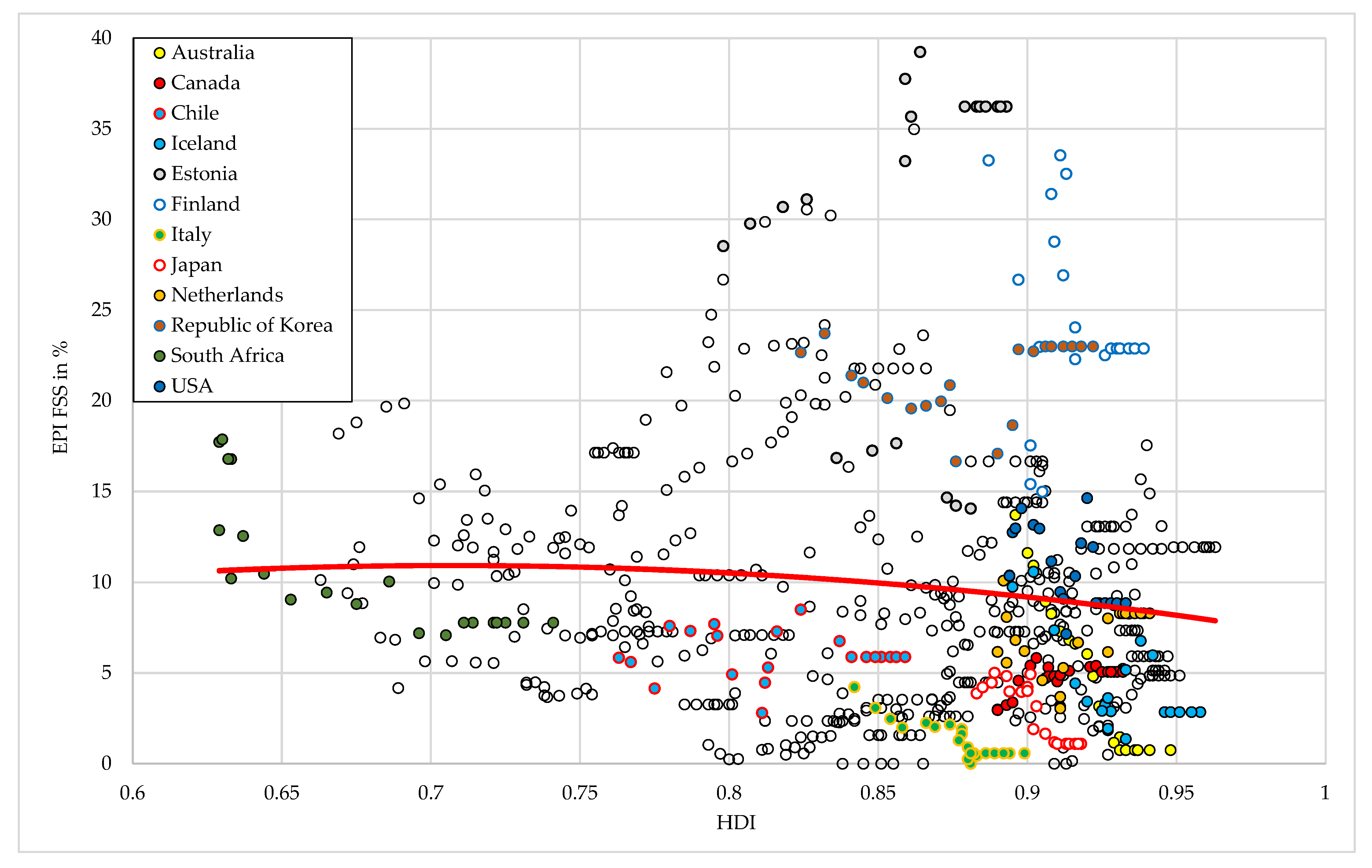
The graphical representation of the raw data and the resulting modeled EKC in the form of a ∩-shaped parabola is represented in Figure 1.

The turning point of the EKC is calculated by taking the first derivative of the function and setting it equal to zero. This yields the following expression:

$$HDI threshold=-{\displaystyle \frac{b}{2a}}=-{\displaystyle \frac{-10.2833}{2·\left(-7.2787\right)}}=0.7$$

(4)

Based on our regression results, this turning point is estimated to occur at an HDI value of approximately 0.7. This indicates that overexploitation of fish stocks increases with development at low HDI levels but begins to decline once a country’s HDI exceeds 0.7, consistent with the theoretical EKC hypothesis.

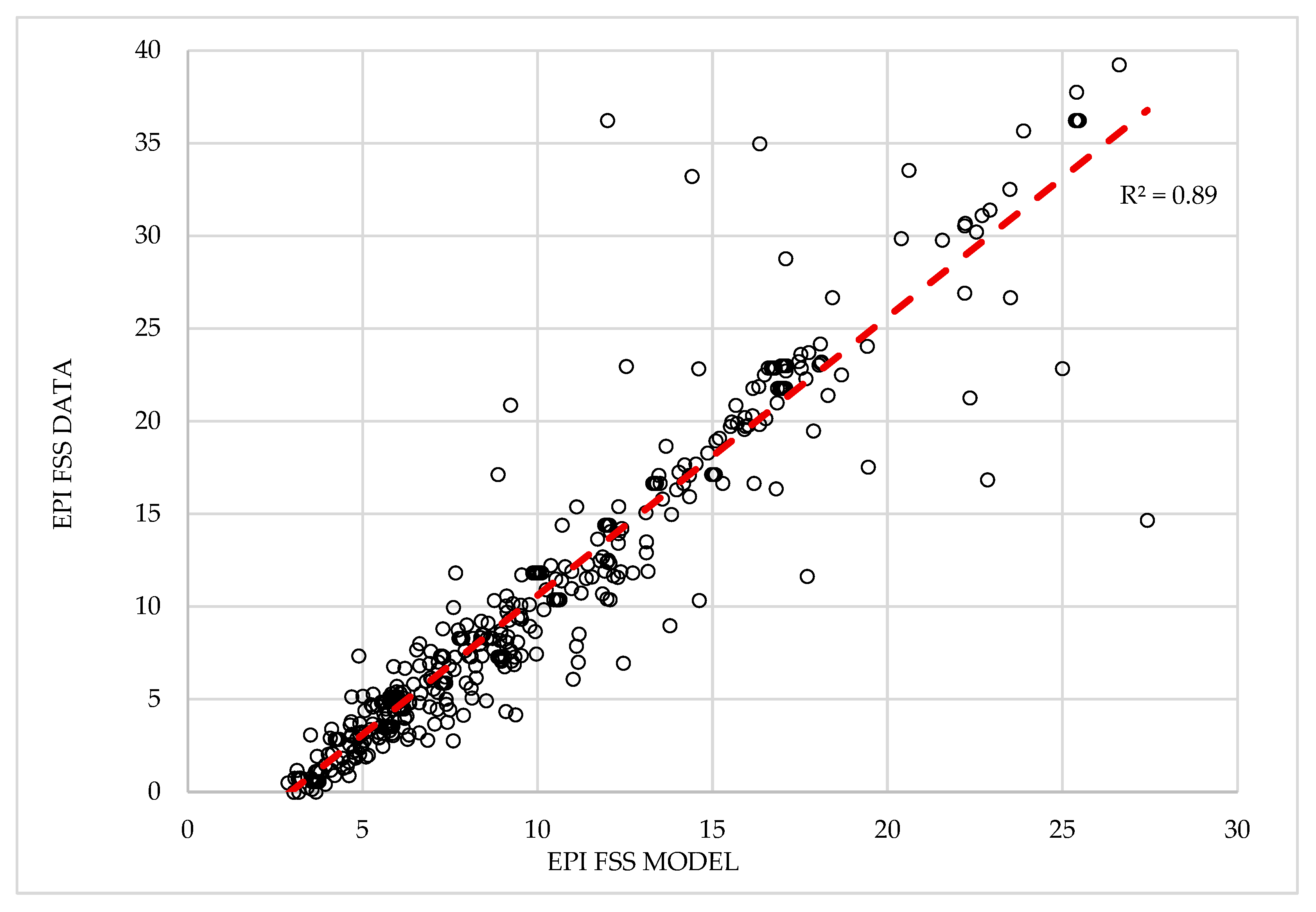
Figure 2 shows the relationship between the predicted fish stock status values obtained from our regression model and the actual observed values from the EPI FSS dataset.

This model shows high predictive accuracy, as shown in Figure 2, where the predicted values well match the observed EPI FSS data (R² = 0.89).

Table 7. GMM FD individual estimation of EPIFSS as a dependent variable.

Variable	Coefficient (β)	Std. Error	t-Statistic	Prob.	S.E. of Regression	J-Statistic	J-Statistic Prob.	AR(1) Prob.	AR(2) Prob.
EPIFSS(−1)	0.678576	0.000485	1400.271	0.0000	2.645127	30.81462	0.475582	0.1532	0.7404
HDI	−5.664897	0.463821	−12.21355	0.0000
EPIFSS(−1)	0.641688	0.000691	928.9715	0.0000	2.683523	31.78853	0.427037	0.1521	0.6799
FDI	−0.008358	7.82 × 10−5	−106.9069	0.0000
EPIFSS(−1)	0.613472	0.005685	107.9082	0.0000	2.688377	31.18057	0.457140	0.1793	0.7754
R&D	−2.679301	0.155328	−17.24926	0.0000
EPIFSS(−1)	0.594156	0.001459	407.2611	0.0000	2.620104	30.31879	0.449417	0.1778	0.6287
EDU	−0.395378	0.014293	−27.66317	0.0000
EPIFSS(−1)	0.632962	0.000403	1572.540	0.0000	2.669595	32.30335	0.402158	0.1602	0.7488
EPICDA	−0.020434	0.001981	−10.31513	0.0000

Method: Panel Generalized Method of Moments. Transformation: First Differences. Sample (adjusted): 2002–2020. Periods included: 19. Cross-sections included: 33. White period standard errors and covariance (d.f. corrected). Instruments: @DYN(EPIFSS,-2) EPIFSS.

shows the negative linear correlation between the EPIFSS as a dependent variable and HDI, FDI, R&D, EDU, and EPICDA as independent and separate regressors taken one by one, in isolation.

Table 7 contains the results of the GMM estimation in first differences for individual regressors, using EPI fish stock status (EPIFSS) as the dependent variable. Each specification includes an explanatory variable alongside the lagged dependent variable to isolate its effect on the sustainability of the fishery. The coefficient for the human development index (HDI) is negative and highly significant (−5.665, p < 0.01), indicating that higher human development levels are associated with a lower share of collapsed stocks in total catch, reflecting improved fisheries outcomes. Similar negative and statistically significant effects are found for foreign direct investment (FDI), research and development (R&D), education expenditure (EDU), and carbon-adjusted CO₂ intensity (EPICDA), suggesting that investment in innovation, human capital, and sustainable practices supports healthier fish stocks.

In all models, the lagged EPIFSS variable remains highly significant, with coefficients ranging from 0.594 to 0.679, underscoring the persistence and path dependence of fish stock dynamics. Model diagnostics confirm the robustness of the results: Hansen J-statistics yield p-values between 0.40 and 0.48, supporting instrument validity, while Arellano–Bond tests show no evidence of first- or second-order serial correlation (AR(1) p > 0.15; AR(2) p > 0.62). Overall, the results emphasise the role of development-related investments in promoting the sustainable use of marine resources and curbing overfishing.

To further explore the relationship between structural factors and fisheries sustainability, we regress EPIFSS on carbon dioxide emissions per capita (EPICDA), foreign direct investment (FDI), and research and development expenditure (R&D) (

Table 8. GMM estimation of EPIFSS on EPICDA, FDI, and R&D.

Variable	Coefficient	Std. Error	t-Statistic	Prob.
EPIFSS(−1)	0.565134	0.009751	57.95370	0.0000
EPICDA	−0.029534	0.009102	−3.244793	0.0028
FDI	−0.010231	0.000635	−16.12381	0.0000
R&D	−2.652183	0.201391	−13.16933	0.0000
Mean dependent var	−0.152042	S.D. dependent var		2.542035
S.E. of regression	2.660375	Sum squared resid		4112.084
J-statistic	28.04626	Instrument rank		33
Prob(J-statistic)	0.515440

Method: Panel Generalized Method of Moments. Transformation: First Differences. Sample (adjusted): 2002–2020. Periods included: 19. Cross-sections included: 33. Total panel (unbalanced) observations: 585. White period instrument weighting matrix. Instruments: @DYN(EPIFSS,-2).

).

Table 8 shows the results of the Arellano–Bond GMM estimation in first differences. The significant positive coefficient for the lagged dependent variable (β = 0.565, p < 0.001) confirms the persistence of fish stock status over time. All explanatory variables are significant and have a negative sign, indicating that lower CO₂ emissions (EPICDA), higher foreign direct investment (FDI), and higher research expenditure (R&D) are associated with an improvement in fish stock sustainability. The model passes the main diagnostics, with the J-statistic (p = 0.515) confirming the validity of the instruments. Table 8 presents the Arellano–Bond tests for autocorrelation. Both AR(1) (p = 0.230) and AR(2) (p = 0.733) are statistically insignificant, indicating no evidence of first- or second-order serial correlation in the residuals. This supports the validity of the GMM estimator.

Lastly, we regress EPIFSS on carbon dioxide emissions per capita (CDA), human development index (HDI), and foreign direct investment (FDI) (

Table 9. GMM estimation of EPIFSS on EPICDA, HDI, and FDI.

Variable	Coefficient	Std. Error	t-Statistic	Prob.
EPIFSS(−1)	0.604971	0.002322	260.5191	0.0000
EPICDA	−0.023643	0.007850	−3.011819	0.0050
HDI	−7.581537	1.736215	−4.366705	0.0001
FDI	−0.009234	0.000291	−31.75257	0.0000
Mean dependent var	−0.137010	S.D. dependent var		2.464595
S.E. of regression	2.654260	Sum squared resid		4389.096
J-statistic	31.13940	Instrument rank		33
Prob(J-statistic)	0.358882

Method: Panel Generalized Method of Moments. Transformation: First Differences. Sample (adjusted): 2002–2020. Periods included: 19. Cross-sections included: 33. Total panel observations: 627. White period standard errors and covariance (d.f. corrected). Instruments: @DYN(EPIFSS,-2).

).

The results of the GMM estimation in Table 9 confirm the persistence of fish stock status over time, with a highly significant and positive coefficient for the lagged dependent variable (β = 0.605, p < 0.001). All explanatory variables are statistically significant and have a negative sign, indicating that reducing carbon emissions (EPICDA), improving human development (HDI), and increasing foreign direct investment (FDI) are associated with improved sustainability of fish stocks. The negative coefficient for HDI (β = −7.582, p < 0.001) reflects the broader role of socio-economic development in supporting marine conservation outcomes. Diagnostic tests confirm the robustness of the model: the J-statistic is not significant (p = 0.359), and the Arellano–Bond tests for AR(1) p = 0.1517 and AR(2) p = 0.7012) do not reject the null hypothesis of no autocorrelation in the residuals, confirming the consistency of the GMM estimator.

5. Discussion

The results of this study provide convincing evidence for an inverted-U-shaped environmental Kuznets curve (EKC) related to the sustainability of marine resources. The negative coefficient for the HDI² and the positive coefficient for the HDI indicate that economic and human development initially contribute to overexploitation of stocks, but lead to an improvement once a certain development threshold is crossed. This result is consistent with traditional EKC applications in pollution studies [4,5], but offers important new insights into renewable marine resources.

As far as we are aware, no previous study has quantitatively analyzed the relationship between the human development index (HDI) and the state of fish stocks using the EKC framework, making this analysis a pioneering contribution. Additional support is provided by Amorim et al. [39], who also relied on the HDI and its quadratic transformation to analyze fish stocks in a data-constrained context. Their multinomial regression found that the probability of underutilization is highest in countries with medium HDI (around 0.70–0.80). Although its methodological approach is similar to the logic of the EKC [4], it uses FAO-based criteria instead of the EPIFSS indicator. Nevertheless, both studies show similar non-linear development and resource dynamics. Future research should further analyze the underlying mechanisms, taking into account indicators such as per capita fish consumption, trade balances, and the effectiveness of fisheries policies.

The significant negative associations between EPIFSS and foreign direct investment (FDI), education (EDU), and research and development (R&D) expenditure emphasise the importance of institutional and structural factors. These findings echo previous studies showing that investment in human capital and technological innovation improves environmental governance and enforcement capacity [18,19]. The persistence of the state of fish stocks emphasises the long-term nature of ecological degradation and recovery processes.

The delayed recovery of fishery resources is due to two key factors. Firstly, marine ecosystems may exceed ecological thresholds at which it becomes increasingly difficult to reverse degradation without a significant reduction in fishing pressure. Secondly, policy response is often delayed due to slow institutional adaptation and limited implementation of science-based management. Effective recovery, therefore, requires timely, evidence-based management and explicit recognition of ecological constraints and non-linear feedbacks that characterize marine systems [40].

Carbon dioxide emissions, measured here by the EPICDA variable (carbon-adjusted CO₂ emissions per capita), contribute directly to ocean acidification and threaten marine primary producers such as phytoplankton. As primary producers, phytoplankton support almost all fish species either directly or indirectly through intermediate trophic levels [41]. Excess atmospheric CO₂ lowers ocean pH, disrupts carbonate chemistry, and affects nutrient cycling, light availability, and phytoplankton metabolism [42]. These changes reduce primary productivity and alter community composition, weakening fisheries yields and limiting long-term sustainability. The negative relationship between EPICDA and EPIFSS shows that limiting carbon emissions is crucial not only for mitigating climate change but also for maintaining sustainable fisheries. These results highlight the complexity of the relationship between development and sustainability and emphasise the need for targeted policy measures such as marine monitoring, education, and sustainable practices, rather than relying on economic growth alone.

Future research should extend this analysis by including additional indicators that reflect the dynamics of the global seafood market, such as per capita fish consumption and trade balance, which reflect dietary habits and import dependence. For example, countries with a high HDI may manage domestic stocks sustainably but indirectly contribute to global overfishing through imports—a phenomenon aligned with the concept of telecoupling, where distant ecological and socio-economic systems are interconnected through global trade. In such cases, consumer demand in one country can drive intensive fishing or aquaculture production in another, often resulting in environmental degradation—such as habitat destruction, pollution, or overexploitation—that is effectively displaced across national borders [43,44].

The EKC turning point for the sustainability of fish stocks estimated in this analysis is approximately at an HDI of 0.7, which is consistent with similar studies [17]. This convergence suggests that environmental pressures could decrease once countries reach comparable levels of institutional maturity, education, and innovation.

6. Conclusions

This paper analyzed the relationship between economic development and the sustainability of fish stocks using panel data from 32 economies (2002–2020). The results confirm the existence of an inverted-U-shaped environmental Kuznets curve (EKC) in relation to the human development index (HDI), suggesting that marine ecosystems initially deteriorate with development but begin to recover as institutional and technological capacities improve. Foreign direct investment (FDI), education, and expenditure on research and development (R&D) were found to be important determinants of the sustainability of fish stocks. These factors, often overlooked in conventional EKC analyses, highlight the institutional and knowledge-based mechanisms that are critical to ecological recovery. Countries that are at or beyond the EKC tipping point thus have the potential to reverse ecological degradation through targeted, sustainable investments.

From a policy perspective, these results make it clear that economic growth alone is not enough to ensure ocean sustainability. Effective environmental management requires proactive strategies that combine development with education, innovation, and international co-operation.

This study has limitations, including possible data limitations and inconsistencies in measurements across countries. An important limitation of this study is the absence of important policy variables, such as the intensity of fisheries subsidies, the extent of marine protected areas, and the share of aquaculture production. Although these factors are important for understanding institutional and policy impacts on fisheries sustainability, they were excluded due to limited data availability and consistency across countries and time. Future research should aim to include these variables to better assess the impact of targeted policy instruments on fish stock outcomes.

Nevertheless, the results are consistent with previous EKC findings in other environmental contexts. For example, using a comparable GMM approach, Mance et al. [17] found a similar inverted-U-shaped relationship between the HDI and pesticide use in EU agriculture and emphasised that environmental improvements are not automatic outcomes of growth, but depend on strategic investments in education, innovation, and governance. Taken together, these results emphasise the crucial role of development quality, alongside economic growth, in achieving sustainable environmental outcomes.