Scheduling and Routing of Device Maintenance for an Outdoor Air Quality Monitoring IoT

Abstract

Air quality monitoring IoT is one of the approaches to achieving a sustainable future. However, the large area of IoT and the high number of monitoring microsites pose challenges for device maintenance to guarantee quality of service (QoS) in monitoring. This paper proposes a novel maintenance programming model for a large-area IoT containing 1500 monitoring microsites. In contrast to classic device maintenance, the addressed programming scenario considers the division of appropriate microsites into batches, the determination of the batch maintenance date, vehicle routing for the delivery of maintenance services, and a set of hard constraints such as QoS in air quality monitoring, the maximum number of labor working hours, and an upper limit on the total CO₂ emissions. Heuristics are proposed to generate the batches of microsites and the scheduled maintenance date for the batches. A genetic algorithm is designed to find the shortest routes by which to visit the batch microsites by a fleet of vehicles. Simulations are conducted based on government open data. The experimental results show that the maintenance and transportation costs yielded by the proposed model grow linearly with the number of microsites if the fleet size is also linearly related to the microsite number. The mean time between two consecutive cycles is around 17 days, which is generally sufficient for the preparation of the required maintenance materials and personnel. With the proposed method, the decision-maker can circumvent the difficulties in handling the hard constraints, and the allocation of maintenance resources, including budget, materials, and engineering personnel, is easier to manage.

1. Introduction

The industrialization and urbanization of human society have not only boosted economic growth but also led to the emission of large volumes of air pollutants. Air pollution is one of the key factors resulting in global warming and climate change, causing tremendous damage to the natural environment. Ambient aerosols, especially particulate matter with an aerodynamic diameter ≤ 2.5 μm (PM_2.5), have led to premature deaths due to respiratory diseases [1,2] and cancer [3]. Following the establishment of the Kyoto Protocol in 1997 and the Paris Agreement in 2015, the member countries gathered at COP27 (https://www.un.org/en/climatechange/cop27, accessed on 1 November 2023) in 2022 announced a historical decision to create a loss and damage fund. However, the fundamental issue for carbon reduction remains unsolved due to the hesitation of major carbon-producing countries in reducing the use of fossil fuels. It is anticipated that air pollution will remain a major challenge in achieving a sustainable future.

To address the above, the Taiwanese Ministry of Environment (MOENV) has built an Internet of Things (IoT) connecting 78 supersites for air quality monitoring. These supersites are very costly, and most of them are deployed only in densely populated regions and industrial complexes. These facilities provide a macro view for the city-level and district-level inspection of air quality, rather than a micro perspective of people’s livelihoods for the detection of local air pollution. In contrast, microsites are composed of cheap sensors that measure the quantities and sizes of suspended air particles, but they are not able to analyze the compositional elements of particles. Due to their low-cost and low-power nature, microsites can be intensively deployed in wider regions, including rural areas. After appropriate measure calibration [4], the data collected by microsites can be applied alone for specific tasks such as PM_2.5 forecasting and spatiotemporal analysis in communities [5,6,7] or to complement data from supersites to extend their applications [8,9].

However, as the number of air quality monitoring microsites is significantly increasing, the operation and maintenance (O&M) of these sensors becomes highly challenging. A prudent maintenance strategy can not only improve the working efficiency of equipment but also reduce the costs and resources required for maintenance activities. There are two classic maintenance policies, namely corrective maintenance (CM) and preventive maintenance (PM). CM involves maintenance activities performed only when equipment halts operation due to failure. Therefore, CM is passive and responsive to unplanned events that incur high costs and prolong the system’s breakdown if no anticipated maintenance plan has been created to prevent or predict such equipment faults. On the other hand, PM involves creating an anticipated plan based on the estimated time between equipment failures such that appropriate maintenance tasks can be performed prior to expected failures. Thus, PM is proactive and programmable, seeking to avoid expected failures before they take place. As compared to CM, PM requires additional programming costs to formulate appropriate plans and preventive operational costs to sustain the equipment’s working performance. PM trades in these additional costs for improved equipment lifetimes and operational efficiency, reducing the necessity of expensive CM operations. The allocation of maintenance resources such as personnel, equipment, materials, operation time, and budget can be better managed with PM. Meanwhile, IoT has been considered as a viable tool to predict equipment failures in manufacturing systems [10]; however, this has never been addressed in the literature.

The huge number of microsites in the air quality monitoring IoT creates more challenges for device maintenance than that observed in manufacturing systems. These challenges include at least the following. Firstly, in classic manufacturing systems, the machines operate in a serial or parallel fashion. The system’s overall reliability is estimated based on the reliability of individual machines and their coupled architecture. However, in the air quality monitoring IoT, a microsite sensor failure will not immediately cause the IoT’s breakdown but will reduce the service availability. A measurement standard for the quality of service (QoS) of the air quality monitoring IoT needs to be defined such that the criticality of a microsite failure can be gauged. Secondly, in contrast to classic manufacturing systems, where the amount of equipment is small, the air quality monitoring IoT contains thousands of microsites. Thus, it is necessary to group the microsites into batches, which should be scheduled for maintenance on appropriate dates in order to sustain satisfactory IoT QoS with the minimum maintenance cost. However, the batch grouping and maintenance scheduling of microsites is an exponential combinatoric problem that requires appropriate heuristics to find near-optimal solutions. Thirdly, in traditional maintenance scenarios, the devices are located within close proximity, such as inside a factory. In contrast, air quality monitoring microsites span a large geographical area, such as a city or a rural county. A fleet of engineering vehicles needs to be reserved to carry sufficient labor and materials to perform maintenance operations. The sequence of the chosen microsites assigned to each on-duty vehicle to perform maintenance is critical to shorten the vehicle traveling distance, satisfy the allowable labor working hours in a day, and reduce the transportation cost. This problem is known as the vehicle routing problem, which is NP-hard [11]. Again, an effective heuristic is needed to find the near-optimal shortest route. Fourth, the main type of air pollution is carbon dioxide (CO₂) emissions from vehicles. In the air quality monitoring IoT service, it is essential to reduce the CO₂ emissions generated by the engineering vehicles visiting the microsites for maintenance. CO₂ reduction can be implemented as a constraint or incorporated into the objective cost. This paper aims to propose novel solutions to the above-noted challenges regarding maintenance scheduling and routing for the outdoor air quality monitoring IoT. The scientific novelty of this paper lies in the proposal of the first formulation of the problem and the linkage between innovative algorithms and industrial practice.

2. Literature Review

The maintenance context for a classic business and the air quality monitoring IoT is different in several aspects, as previously noted. However, the literature has mainly focused on equipment maintenance for traditional businesses, while the specific features of IoT maintenance have been overlooked. In the following, we describe the scenario of the air quality monitoring IoT implemented in Taiwan and review the main literature on classic equipment maintenance.

2.1. Air Quality Monitoring IoT in Taiwan

Most of the supersites are installed near the west coast, where industrial districts and megacities are located, as shown in Figure 1a. These supersites are high-cost and can measure the masses of several types of ambient aerosol particles. The Taiwanese MOENV has implemented two types of mass-measuring approaches at the supersites [12]. The gravimetric method [13] requires manual effort to prepare special filters, collect suspended particle samples, store and maintain sample quality, and measure the weights of particles with designated sizes. The beta-attenuation method [14] emits Carbon-14 (¹⁴C) radiation that is passed through a glass filter with or without a sample. The beta ray is decreased when it passes through particle samples, and the difference between the two filters is gauged to calculate the particle mass. These supersites are equipped with analyzers for various chemical elements, including CO, O₃, SO₂, and NO₂. This information is necessary for the identification of emission sources. However, due to the high implementation cost, the supersites are sparsely distributed and facilitate only a macro view for large-area air quality monitoring, rather than a micro view for the measurement of air pollution concentrations within local households.

Research institutes and private companies have constructed several IoTs consisting of microsites to achieve a finer-grained resolution for air quality monitoring. As of the end of 2024, there were more than 10,300 state-supported microsites implemented over Taiwan, as shown in Figure 1b. These microsites use low-cost sensors (LCSs), which only measure the masses of aerosol particles and are not able to identify the compositional elements of the pollution, because the technology used by the LCSs is simple. Laser light scattering (LLS) and the quartz crystal microbalance (QCM) are two widely used technologies for the implementation of LCSs [8]. By emitting a laser beam to particles to generate light scattering, LLS tools detect the light at a certain angle to estimate the particle size and the number of particles. Meanwhile, a QCM measures the difference in the frequency of the quartz crystal on the oscillator with and without the pollutant to estimate the particle mass. Moreover, LCSs are not highly accurate and thus need to be calibrated with reference to nearby supersites [15].

To ensure the high usability of the air monitoring IoT, the on-site equipment must be periodically inspected and sometimes corrected by performing troubleshooting after unexpected failures. A well-managed maintenance plan can improve the working reliability and efficiency of equipment. It not only reduces the expected downtime during operations but also reduces the cost incurred due to equipment replacement following severe failures. Because the supersite equipment is complex and requires long-term maintenance, and also because the distance between supersites is large, the maintenance of each supersite is independently dealt with by a government agent, and no batch maintenance plan for multiple supersites is needed. In contrast, the distance between microsites is usually less than 1 km, and on-site maintenance takes less time because of the use of simple technology. For microsites, it is easier for their maintenance plan to be formulated collectively on a batch basis to save costs and labor, reducing the vehicle traveling distance and the number of maintenance days. However, there are a great number of microsites. It thus becomes challenging to design a minimum cost algorithm to determine the date to conduct each batch’s maintenance and the subset of microsites to be included in the batch. Moreover, as maintenance is performed on a batch basis, a vehicle routing algorithm is needed to deliver maintenance services to each microsite contained in the batch. The routing algorithm needs to be able to minimize the overall cost while satisfying a set of practical constraints, such as the labor working time, vehicle fleet size, IoT service availability, and vehicle CO₂ emissions.

2.2. Maintenance Scheduling Policies

Where there is business, there is maintenance. Business involves equipment or software platforms, which enable manufacturing or provide services to customers. Maintenance is planned and performed to reduce equipment or software breakdowns and maximize the business benefits. In traditional manufacturing, there are production lines on which equipment or devices are located and operated. To fulfill the business process efficiently, it is necessary to increase the manufacturing uptime and reduce the delay due to equipment failures. Maintenance is a viable means of preventing a failure before it occurs or detecting and fixing failures before they result in business disruptions. There are a variety of maintenance tasks, such as inspection, cleaning, adjusting, lubricating, repair, replenishing, upgrades, fault diagnosis, and replacement. Some of these maintenance tasks, like cleaning, adjusting, and lubricating, are relatively low-cost, but some can be very expensive, like the repair or replacement of a wind turbine blade due to an identified crack. Maintenance focuses on developing strategic policies and tactical methodologies for the avoidance of equipment failures, which progressively lead to system breakdowns [16]. There are two main maintenance policies—corrective maintenance and preventive maintenance—as described below.

A.

Corrective Maintenance (CM)

In CM, maintenance operations such as repair and replacement are conducted only when equipment halts operations due to failure. Thus, CM is passive and responsive, and it can lead to high maintenance costs and lengthen the system breakdown time. If a CM policy is practiced, it is challenging to plan the allocation of maintenance resources in advance, and a high level of QoS cannot be assured. The advantage of CM is that there is no need to shut down the system to execute scheduled maintenance prior to possible failures.

B.

Preventive Maintenance (PM)

Any maintenance that is not CM can be viewed as an instance of PM. PM plans for equipment maintenance tasks based on the mean time between failures (MTBF) such that appropriate maintenance tasks can be performed in advance. Therefore, PM is proactive and programmable, aiming to avoid expected failures before they take place. PM considers the age or usage of the deployed components and prescribes periodic or meter-based maintenance with a programmed plan. The optimal maintenance time interval suggested by the plan is determined by an optimization method to extend the components’ MTBF. In order to facilitate PM, the calculation for the reliability of the components and the entire system needs to be modeled. Then, an optimization method is adopted to determine the optimal PM interval, leading to an accepted system reliability measurement based on the model. As compared to CM, PM requires additional programming costs to create appropriate plans and preventive operational costs to sustain the equipment’s working performance. PM trades in these additional costs for improved equipment lifetimes and operational efficiency, alleviating the need for expensive CM operations. The allocation of maintenance resources such as personnel, equipment, materials, operation time, and budget can be better managed with PM. An emerging trend regarding PM in the context of Industry 4.0 is predictive maintenance (PdM), which records the operational statuses of devices by deploying monitoring sensors [17]. Machine learning approaches can be applied to historical status data to predict the time and type of the next failure of a device, and appropriate maintenance tasks can be executed before the failure happens. Several global experiences and best practices can be found in Camilotti et al. [18]. They reveal the increased benefits achieved via the joint optimization of device reliability and maintenance costs under multiple resource constraints. The existing advanced maintenance practices rely on using IoT sensors to transmit the device working status for the prediction of the next failure. However, a maintenance policy for the IoT sensors themselves has not been described in the literature. The most relevant one may be attributed to Sami and Khan [19], who forecasted the failure rates of IoT smart home devices such as motion sensors, door sensors, smoke sensors, cameras, locks, etc. Historical data on the sensor status (failure or not) in response to user actions or automation is recorded. The time series of the device failure rate is then produced from the historical data by counting the number of failures per 20 attempts in 10 min. The next failure time is forecasted by applying bi-directional long short-term memory (Bi-LSTM) and a gated recurrent unit (GRU) to the time series.

However, the method proposed by Sami and Khan [19] does not align with our problem scenario. Firstly, smart home devices exhibit different functionalities, and the failure of a device reflects the missing delivery of a service. By contrast, the air quality monitoring IoT is considered a service as a whole, and one sensor’s failure will not cause the complete failure of the service. The system has a degree of tolerance for sensor failures. Secondly, the number of home device failures is counted based on requests. In our problem context, air quality monitoring is continuously requested automatically. The continuous failure of a sensor due to multiple requests within a time period should not be considered as many failures because the device cannot be fixed or replaced in such a period. Thirdly, the number of smart home devices is small, and these devices are located at the same place. However, the air quality monitoring IoT contains thousands of sensors scattered across a large geographical space, and an effective vehicle routing optimization scheme is needed to complete the maintenance task within the allowable working hours.

Different maintenance planning policies lead to various maintenance costs and system risks. CM has no cost for failure prevention. However, once a failure occurs, the failed component is usually non-repairable and needs to be replaced. Sometimes, the failed component may result in the propagation of a disaster, which can cause tremendous system losses. Therefore, CM may have the highest maintenance cost. By contrast, PM involves prevention costs to conduct periodic or meter-based maintenance. Benefitting from the scheduled maintenance, the MTBF is extended, and the cost for repair and replacement is reduced. As each business has different types of equipment and cash flows, there exists no best maintenance policy for all businesses. By leveraging the maintenance cost and resource constraints (such as cash flow, repair and replacement parts, and labor), businesses that implement a robust and sound maintenance policy can gain benefits such as decreased business downtime, lengthened equipment lifetimes, lower costs to maintain essential equipment in the long term, and lower energy consumption due to the high level of machinery efficiency.

2.3. Maintenance Scheduling Methodologies

In contrast to CM, PM requires an optimization methodology to produce the optimal maintenance schedule. The applied methodologies in the literature fall into five main categories as follows.

A.

Mathematical Programming

Mathematical programming is the earliest presented approach in the literature for the optimization of PM plans. Mijailovie [20] proposed a probabilistic method to derive the optimal PM period by minimizing the cost per unit of time. Two types of component failures are considered: the wear-out failure and the chance failure, modeled by a Weibull distribution and an exponential distribution, respectively. As compared to PM scheduling using a fixed PM interval, the cost-based probabilistic method achieves a lower overall cost for a given time span. Zhao [21] presented a PM policy that activates a new PM cycle by allowing the same number of failures in the time intervals between neighboring cycles, such that a critical reliability level is achieved during the operating time. The optimal PM time interval is calculated by a recursive function considering the cost, reliability, hazard rate, and system availability between neighboring cycles. In Nourelfath et al. [22], production, maintenance, and quality are integrated into an optimization model. The model’s objective is to minimize the cost subject to the production demand, PM plan, and product quality control costs. An iterative optimization algorithm is developed to tackle the constrained model. Su and Tsai [23] present PM planning for a two-parallel-machine problem to minimize the production makespan. The two machines must be shut down for maintenance. A mixed-integer programming model is developed to determine the optimal maintenance time and job sequencing during production.

B.

Artificial Intelligence

Artificial Intelligence (AI) is emerging as a popular solution method for the optimization of PM scheduling. The most notable and prevailing ones are genetic algorithms (GAs), simulated annealing (SA), and ant colony optimization (ACO). Tsai et al. [24] proposed a GA for the cost reduction and reliability improvement of a single system with multiple components. The GA is applied to determine which PM activities should be performed at every PM cycle, where the activities are categorized as simple maintenance, corrective repair, preventive replacement, and corrective replacement. The objective of the GA is to determine the activity combination that fits the maximum life per maintenance cost. Van et al. [25] adopted batch PM scheduling, where the PM activities of multiple components are combined rather than being performed separately. The authors applied both GA and MULTIFIT optimization algorithms to group PM activities with the repairmen availability constraint. The GA is applied to find the optimal PM batch, while MULTIFIT is performed to identify the optimal assignment of PM activities to maintenance components. Mahadevan et al. [26] combined a GA and SA to obtain the optimal PM schedule by assigning PM tasks to critical components. The objective function considers variables including the time and costs for replacement, repair, downtime, failure, and standby. Samrout et al. [27] used the ant colony optimization (ACO) algorithm to minimize the PM cost function under a given availability constraint. The system availability is calculated using a Monte Carlo simulation approach. ACO determines the optimal solution vector for the component inspection period. The additional problem of reliability assurance is also resolved.

C.

Multi-Objective Approaches

Multi-objective approaches have been employed for PM scheduling with multiple optimization goals. Adhikary et al. [28] adopted a multi-objective genetic algorithm (MOGA) to maximize the system’s availability and minimize the maintenance cost. A case study on a coal-fired boiler tube problem was illustrated. The experimental results showed that the MOGA could improve both objective terms. Wang and Liu [29] studied a production problem with machines and molds on which PM activities were performed. The second version of the non-dominated sorting genetic algorithm (NSGA-II) was adopted to approach the Pareto front. The non-dominated solutions at the front suggested a trade-off between the production makespan and the machine and mold unavailability due to PM operations.

D.

Others

In addition to the previously noted maintenance scheduling methodologies, some existing works have selected miscellaneous approaches. For instance, Alabdulkarim et al. [30] studied the characteristics of simulation-based approaches for maintenance scheduling in the manufacturing industry. Simulation-based maintenance approaches conduct the simulation of variables separately, demonstrating discrepancies with regard to reality. Alabdulkarim et al. [30] simultaneously simulated the uncertain forecasting of asset failures, maintenance costs, and inventory availability in a manufacturing system via the Monte Carlo simulation approach. The dependency between uncertain variables and the impact on the overall system could be estimated. Criticality-based approaches provide another opportunity for efficient maintenance. Ab-Samat et al. [31] conducted a case study where the number of maintenance personnel was limited, and previous PM practices could not prevent unplanned system breakdowns. By applying critical analysis, a tree diagram was used to represent the current PM activities and the criticality of the unplanned failure. Then, a more efficient PM schedule was generated from the outcome of the analysis.

3. Proposed Method

3.1. Studied Problem

As the number of microsites is tremendous and they span large areas to provide a finer-grained spatial resolution for air quality monitoring, the O&M of these microsites was segmented into several geographical districts based on their locations. The O&M practiced in each district is individually managed by the contract company. This paper investigates the Central Taiwan air quality district, where there are over 1500 microsites distributed in Taichung City, Changhua County, and Nantou County, as shown in Figure 2. With such a large number of microsites, it becomes laborious and costly to perform maintenance across the microsite IoT. As the number of microsites will continue to grow in the future, it becomes critical for the contract company to develop optimization programming models to execute the maintenance task in a manner that is low-cost and efficient and guarantees QoS.

The current maintenance strategy adopted by the contract company consists of fixed-time PM intervals for randomly chosen microsites and responsive CM for unexpected microsite failures. This maintenance strategy does not allow for appropriate resource allocation or guarantee IoT service availability. The occurrence of unexpected microsite failures can be more frequent, and the downtime of failed microsites is lengthened. Moreover, it increases the sensor replacement cost and reduces IoT service availability, which would both be avoidable if a more intelligent maintenance strategy was implemented. We anticipate that robust maintenance programming for the air quality monitoring IoT should at least meet the following criteria. Firstly, the IoT service availability needs to be defined and estimated such that the tangible QoS can be measured. Secondly, the capacity of the maintenance resources is limited. The schedule produced by maintenance programming should respect the resource constraint. Thirdly, the vehicle routing time for visiting the scheduled microsites, plus the time required to perform maintenance activities, should be no greater than the allowable working time in a day.

A typical microsite deployed in the Central Taiwan air quality district consists of several types of sensors and ancillary devices such as fans, a power supply, and networking components, all mounted on a pole, as shown in Figure 3. These sensors monitor environmental data including PM_2.5, PM₁₀, the temperature, the relative humidity, the total volatile organic compounds (TVOC), and the wind speed and direction. In the following, we refer to a microsite with all its sensors and ancillary devices as a single composite unit for maintenance, without breaking it down into individual sensors and devices, because all these sensors are at the same location and the maintenance engineer can inspect all sensors and devices at one time to perform the necessary maintenance activities.

3.2. Maintenance Programming Framework

In the following, we elucidate on the reliability evaluation of the sensors, the definition of IoT service availability, the scheduling and routing of microsite IoT maintenance, the proposed maintenance programming model, and the algorithms to determine the near-optimal solution of the model. Finally, a visualization-based user interface is developed.

Table 1. Nomenclature.

Notation	Description
n	Number of microsites connected to the air quality monitoring IoT
J	Maximum number of maintenance cycles in the programming
$s_k$	k-th microsite
$t_0^k$	Deployment time of microsite $s_k$
${\lambda }_j^k$	Failure rate of microsite $s_k$ within the j-th maintenance cycle
$R_k\left(t\right)$	Reliability of microsite $s_k$ by time t
$m_j$	Improvement factor for the j-th maintenance cycle
$\mathcal{R}\left(s_i\right)$	Availability of microsite $s_k$
$\widehat{\mathcal{R}}\left({\bigcup }_{i=1}^n{s}_i\right)$	Normalized availability of the IoT service
Xi	Batch of visited microsites in the i-th maintenance cycle
Yi	Set of links between any ordered pairs of microsites from Xi
$z_{v,k_1,k_2,j}$	$z_{v,k_1,k_2,j}=1$ indicates that vehicle v passes through the link connecting $s_{k_1}$ and $s_{k_2}$ during the j-th maintenance cycle, and $z_{v,k_1,k_2,j}=0$ otherwise
$e_{v,k_1,k_2}$	Amount of CO2 emitted from vehicle v passing through the link connecting $s_{k_1}$ and $s_{k_2}$
${\phi }_v$	Fuel efficiency of vehicle v
${\sigma }_v$	Mean speed of vehicle v
${\delta }_{fuel}$	Cost per liter of fuel
$C_{PM}\left(x_{kj}\right)$	PM cost for microsite $s_k$ in the j-th maintenance cycle
$C_{CM}\left(x_{kj}\right)$	CM cost for microsite $s_k$ in the j-th maintenance cycle
$C_{Tran}\left(k_1,k_2\right)$	Transportation cost for vehicle v passing through link $\left(k_1,k_2\right)$
$t_{PM}$	Mean operational time for performing PM activities at a single site
$t_{CM}$	Mean operational time for performing CM activities at a single site

tabulates the nomenclature that will be referred to in the remainder of this paper.

3.2.1. Reliability Evaluation of Microsites Prior to Maintenance

As previously noted, maintenance focuses on developing strategic policies and tactical procedures for the avoidance of component failures, which progressively lead to system breakdowns. In the case of the IoT providing air quality monitoring, the definition of system breakdown needs to be amended in terms of the IoT service availability, since the air quality monitoring IoT still functions in parts if there is at least one microsite successfully transmitting its air pollution measures to the IoT hub. In other words, a system breakdown is more appropriately defined by the time at which the IoT availability measure is less than an indicated QoS threshold.

As the IoT was incrementally established depending on the allocated budget, the selected microsites for a PM batch may be of different ages. Let s_k denote microsite k, which was deployed at time $t_0^k$. We can calculate the failure rate ${\mathsf{\lambda }}_k$ of s_k as ${\mathsf{\lambda }}_k=1/{\theta }_k$, where ${\theta }_k$ is the MTBF suggested from the manufacturer’s in-house test. We follow Shatz’s formulation [32] to estimate the reliability assuming that s_k is operational from its deployment until the current time $t_c$ if no maintenance has ever been performed on s_k as follows:

$$R_k\left(t_c\right)=e^{-{\int }_{t_0^k}^{t_c}{\lambda }_{k}dt}{=e}^{-{\lambda }_k\left(t_c-t_0^k\right)}$$

(1)

3.2.2. Reliability Evaluation of Microsites Between Maintenance Cycles

The lifespan and efficiency of the microsite are improved if appropriate maintenance activities are performed before failures. The activities range from simple PM (such as inspections, cleaning, lubricating, and replenishing of oil) and complex PM (repairing, adjusting, or replacement of some parts) to CM (i.e., entire replacement with a new microsite package). The state of the microsite undergoing maintenance may not be restored to its as-new state but depends on the performed maintenance operations. This constraint is known as imperfect maintenance in the literature [33]. By assuming that the equipment undergoing maintenance activities can operate at a younger age than it is, Tsai et al. [24] defined the improvement factor m_j (0 ≤ m_j ≤ 1), which reduces the age of the equipment after performing the j-th maintenance cycle. Assuming that there are n microsites connected to the IoT and there have been J maintenance cycles already performed at time t₁, t₂, …, t_J, respectively, we denote the set of maintenance batches by $X=\left\{X_j|1\le j\le J\right\}$. For the j-th maintenance cycle, a number of microsites is selected in batch X_j on which to perform maintenance activities. Let $x_{k,j}$ denote the decision variable, where $x_{k,j}=1$ if microsite s_k has been selected in batch X_j and $x_{k,j}=0$ otherwise. Hence, $X_j=\left\{x_{k,j}|x_{k,j}=1\right\}, 1\le j\le J$. The effective age $∆t_k$ of s_k at $t_c$ can be derived as

$$∆t_k=\left(\left(\left(t_1-t_0\right)\left(1-m_1{x}_{k,1}\right)+\left(t_2-t_1\right)\right)\left(1-m_2{x}_{k,2}\right)+\dots +\left(t_J-t_{J-1}\right)\right)\left(1-m_J{x}_{k,J}\right)+\left(t_c-t_J\right)$$

(2)

$$=\left(t_1-t_0\right)\left(1-m_1{x}_{k,1}\right)\left(1-m_2{x}_{k,2}\right)\dots \left(1-m_J{x}_{k,J}\right)+\left(t_2-t_1\right)\left(1-m_2{x}_{k,2}\right)\dots \left(1-m_J{x}_{k,J}\right)+\dots +\left(t_J-t_{J-1}\right)\left(1-m_J{x}_{k,J}\right)+\left(t_c-t_J\right)$$

$$=\sum _{i=1}^J\left(\left(t_i-t_{i-1}\right)\prod _{j=i}^J\left(1-m_j{x}_{k,j}\right)\right)+\left(t_c-t_J\right)$$

where we let ${t_0=t}_0^k$ to simplify the equation. Obviously, the effective age of s_k at $t_c$ is within the following range:

$$\left(t_c-t_J\right)\le ∆t_k \le \left(t_c-t_0\right)$$

(3)

and $∆t_k=t_c-t_J$ if s_k joins the J-th maintenance cycle ($x_{k,J}=1$) and CM is performed on s_k ($m_J=1$). By contrast, $∆t_k=t_c-t_0=t_c-t_0^k$ if s_k does not join any maintenance cycles ($x_{k,j}=0,\forall j$).

Substituting Equation (2) into Equation (1), the reliability of s_k at time $t_c$ (>$t_J$) can be estimated with reference to the effective age of s_k as follows:

$$R_k\left(t_c\right)=e^{-{\int }_{t_0^k}^{t_c}{\lambda }_{k}dt}{=e}^{-{\lambda }_k∆t_k}.$$

(4)

As an illustration of the calculation of the reliability of s_k with several maintenance cycles, an example is given as follows. Let the component MTBF recommended by the manufacturer be 9500 h, so that the initial failure rate is ${\mathsf{\lambda }}_1^k=0.000105$. Assume that three maintenance cycles (M₁, M₂, and M₃) have been performed at $t_1^k$ (=2000 h after deployment), $t_2^k$ (=3000 h), and $t_3^k$ (=3800 h). The scheduled maintenance activities are inspection and cleaning in M₁ (with an improvement factor m = 0.3), part repairs in M₂ (m = 0.5), and part replacements in M₃ (m = 0.8). The reliability of s_k in relation to time t can be estimated by Equation (4). Figure 4 shows the reliability variation of s_k with the three maintenance cycles. It is seen that the reliability starts to gradually deteriorate following its deployment. In M₁, where s_k is still young, simple maintenance activities such as inspection and cleaning are performed, so the reliability is increased because the effective age is improved slightly. As s_k continues to operate, its reliability drops at a faster rate. When the reliability approaches a critical level, another maintenance cycle with necessary part repairs is activated at $t_2^k$. The reliability is restored to an acceptable level and it can remain in good condition for a certain period. When the reliability approaches a critical level again, part replacements are required to reduce the age of s_k and lengthen its lifespan.

3.2.3. IoT Availability Evaluation

The classic PM policy formulates the maintenance schedule based on a fixed time interval or a meter-based measurement. For a wide-area air quality monitoring IoT with many microsites, it is too expensive and time-consuming to perform maintenance on an individual basis. Microsite failures will not immediately shut down the entire IoT service but decrease the effective monitoring area. Thus, a batch maintenance policy is preferred to save costs and time while still simultaneously sustaining a satisfactory IoT service. For a given time instance, different microsites can exhibit varying reliability because they may be deployed at different times and have experienced different cycles of maintenance activities. A decent maintenance programming model should select the most appropriate microsites into a batch for each maintenance cycle such that the QoS of the monitoring IoT can be sustained above a certain level over time. The most appropriate microsites may not simply be those with the lowest reliability but should be chosen with respect to the IoT availability. Figure 5 is a heatmap visualizing the reliability of multiple microsites located at different locations. Each microsite is represented by a circle. The size of the circle reflects the ideal area of monitoring coverage for the microsite, which can be estimated in the calibration phase with reference to a standard supersite [4,15]. The intensity of the red color indicates the reliability value of the corresponding microsite. The redder the circle is, the higher the reliability. As previously noted, the reliability of an air quality monitoring IoT is significantly different from that of a traditional manufacturing system. We develop a new measurement for the evaluation of the QoS performance of an IoT.

In a traditional manufacturing system, various devices may work in serial, parallel, or hybrid mode. The system reliability needs to be evaluated based on the probability that a system breakdown will be caused by the failure of any individual device. However, the traditional methodology for the calculation of the system reliability is not applicable to the case of an air quality monitoring IoT. The reasons are as follows. Firstly, a microsite failure will not cause the immediate breakdown of the IoT system, since the microsites operate independently and data transmission from the other microsites is ongoing. Secondly, the service provided by an air quality monitoring IoT is the delivery of air quality information for a defined monitoring area. Even if multiple microsites fail simultaneously, the monitoring IoT system will still function (albeit imperfectly) with the remaining operational microsites, but it has smaller coverage of the effective monitoring area. By considering the microsite reliability and the IoT coverage area, we propose a new metric called IoT service availability as follows.

As illustrated in Figure 6, let s_i and s_j be two neighboring microsites whose ideal coverage of the monitoring area is represented by a circle with radius r_i and r_j, respectively, and let the distance between s_i and s_j be d_ij. Following previous derivations for microsite reliability after a number of maintenance cycles (see Equation (4)), we define the monitoring availability of microsite $s_i$ (denoted by $\mathcal{R}\left(s_i\right)$) as the multiplication of its reliability and the ideal monitoring coverage at the time of estimation, namely

$$\mathcal{R}\left(s_i\right)=\pi r_i^2{R}_i\left(t_c\right).$$

(5)

By the principles of inclusion and exclusion, we have

$$\mathcal{R}\left(s_i\cup s_j\right)=\mathcal{R}\left(s_i\right)+\mathcal{R}\left(s_j\right)-\mathcal{R}\left(s_i\cap s_j\right)=\pi r_i^2{R}_i\left(t_c\right)+\pi r_j^2{R}_j\left(t_c\right)-\mathcal{R}\left(s_i\cap s_j\right).$$

(6)

If $r_i+r_j\le d_{ij},\mathrm{t}\mathrm{h}\mathrm{e}\mathrm{n}{s}_i\cap s_j=\mathrm{\varnothing }$, leading to $\mathcal{R}\left(s_i\cap s_j\right)=0.$ Otherwise, $\mathcal{R}\left(s_i\cap s_j\right)$ can be obtained by

$$\mathcal{R}\left(s_i\cap s_j\right)=\left(2\pi r_i^2{\displaystyle \frac{{\theta }_i}{2\pi }}+2\pi r_j^2{\displaystyle \frac{{\theta }_j}{2\pi }}-h{d}_{ij}\right)R_{s_i\cap s_j}\left(t_c\right)=\left({\theta }_i{r}_i^2+{\theta }_j{r}_j^2-h{d}_{ij}\right)R_{s_i\cap s_j}\left(t_c\right)$$

(7)

where

$${\theta }_i={\sin }^{-1}{\displaystyle \frac{h}{r_i}}$$

(8)

$${\theta }_j={\sin }^{-1}{\displaystyle \frac{h}{r_j}}$$

(9)

and h should be calculated by resolving the positive root in the following expression:

$$h^2={\displaystyle \frac{4r_i^2{r}_j^2-{\left(d_{ij}^2-r_i^2-r_j^2\right)}^2}{4d_{ij}^2}}$$

(10)

$R_{s_i\cap s_j}\left(t_c\right)$ is the joint reliability of s_i and s_j. Since the operation of s_i and s_j is independent, the monitoring intersection area can be covered if either one of s_i and s_j is operational. Therefore, the joint reliability is the maximum of the separate reliability measures, namely

$$R_{s_i\cap s_j}\left(t_c\right)=\max \left(R_i\left(t_c\right),R_j\left(t_c\right)\right).$$

(11)

For generalization, the availability of the air quality monitoring IoT involving n microsites is as follows:

$$\mathcal{R}\left({\bigcup }_{i=1}^n{s}_i\right)={\sum }_{i=1}^n\mathcal{R}\left(s_i\right)-{\sum }_{i\ne j}\mathcal{R}\left(s_i\cap s_j\right)+{\sum }_{i\ne j\ne k}\mathcal{R}\left(s_i\cap s_j\cap s_k\right)-\dots$$

(12)

$$\pm \mathcal{R}\left(s_1\cap s_2\cap \dots \cap s_n\right)$$

Finally, we define the normalized availability of the IoT, denoted by $\widehat{\mathcal{R}}\left({\bigcup }_{i=1}^n{s}_i\right)$, which falls within the range of [0, 1], such that the decision-maker can ensure the reliability of the IoT service. $\widehat{\mathcal{R}}\left({\bigcup }_{i=1}^n{s}_i\right)$ is calculated by dividing $\mathcal{R}\left({\bigcup }_{i=1}^n{s}_i\right)$ by its maximum value:

$$\widehat{\mathcal{R}}\left({\bigcup }_{i=1}^n{s}_i\right)={\displaystyle \frac{\mathcal{R}\left({\bigcup }_{i=1}^n{s}_i\right)}{\mathcal{R}\left({\bigcup }_{i=1}^n{s}_i|R_i\left(t_c\right)=1,\forall i\right)}}$$

(13)

To ensure the efficiency of calculations using Equation (12) for many microsites, we truncated the calculation after a certain number of intersections. There were 136 intersections truncated from a total of 665 intersections in our calculations, with 1500 microsites. Although the 136 truncated intersections were not directly assessed, they were decomposed into lower-order intersections, and the monitoring availability of the involved microsites was still computed in a lower-order manner. The error percentage compared to using genuine high-order intersections is difficult to estimate. Nevertheless, the final overall availability measure was normalized to the ideal maximum availability, as seen in Equation (13), and both the denominator and numerator were calculated with lower-order intersections; in this way, the error percentage should be reasonable.

3.2.4. Scheduling and Routing of IoT Maintenance

As previously noted, the air quality monitoring IoT has several unique features in contrast to typical manufacturing systems. Unlike the case of manufacturing systems, where the devices are in a factory, the air quality monitoring IoT is supported by many microsites scattered across a wide geographical area. For example, the IoT investigated in our study contains more than 1500 microsites distributed over a 2000 km² area spanning Taichung City, Changhua County, and Nantou County. The maintenance for the microsites in such an IoT has to be managed on a batch basis, rather than on an individual basis, as for a manufacturing system. Then, there arise two problems for the maintenance programming of IoT microsites: (1) batch maintenance scheduling determines the batch maintenance dates in a planning time horizon and selects a batch of microsites for maintenance on each maintenance date; (2) maintenance vehicle routing determines the optimal routes by which to visit the batch of microsites by a fleet of vehicles on each maintenance date. The optimality is defined by an objective function such as cost minimization subject to a set of constraints ranging from the fleet size, labor-hour limit, or QoS availability of the IoT to the maximum CO₂ emissions.

The solution for the maintenance vehicle routing problem depends on the decision-making for the batch maintenance scheduling problem. If two consecutive maintenance dates are far apart, the IoT availability cannot be guaranteed, and more microsites need to be visited for maintenance in vehicle routing. This may cause the violation of the fleet size, labor hour, or CO₂ emission constraints. Moreover, if the microsites of a batch for maintenance are not appropriately selected, the IoT availability cannot be restored to a satisfactory QoS level after performing the maintenance. Therefore, we develop a multiple-run GA with heuristics for the batch maintenance scheduling and routing problems, as will be described in Section 3.2.6.

3.2.5. Maintenance Programming Model

In this section, we present the mathematical formulation of the maintenance programming model. The measures for the considered costs and constraints used in the model are defined as follows.

A.

Maintenance Cost

For each chosen microsite $x_{kj}=1$, to perform the j-th maintenance cycle, there are two situations. If s_k is operational, a preventive maintenance cost $C_{PM}\left(x_{kj}\right)$ is incurred depending on whether simple or complex preventive maintenance is performed. The reliability $R_k\left(t_c\right)$ with which s_k operates during the j-th maintenance cycle can be estimated by using Equation (4). Otherwise, s_k is in breakdown (with the probability estimated by $1-R_k\left(t_c\right)$, and a corrective maintenance cost $C_{CM}\left(x_{kj}\right)$ is incurred to perform the replacement of the entire microsite. The overall maintenance cost $C_1\left(X\right)$ with maintenance programming is calculated as follows:

$$C_1\left(X\right)={\sum }_{j=1}^J{\sum }_{x_{k,j}\in X_j}\left(R_k\left(t_c\right)C_{PM}\left(x_{k,j}\right)+\left(1-R_k\left(t_c\right)\right)C_{CM}\left(x_{k,j}\right)\right)x_{k,j}$$

(14)

B.

Transportation Cost

Let the contract company own a fleet of V engineering vehicles. During the j-th maintenance cycle, some vehicles are dispatched to visit the microsites chosen in the batch $\left\{x_{k,j}|x_{k,j}\in X_j\right\}$. It is desirable to find the shortest overall routes for the on-duty vehicles. This is known as the minimum cost vehicle routing problem (MCVRP), which is NP-hard [11]. Let $Y=\left\{Y_j|1\le j\le J\right\}$ denote the set of feasible vehicle routes traversing the maintenance microsites for each of the J maintenance cycles and $Y_j=\left\{\left(k_1,k_2\right)|x_{k_1,j}{x}_{k_2,j}=1\right\}$ be the set of links $\left(k_1,k_2\right)$ connecting any ordered pairs of microsites in batch $X_j$. Moreover, let $Z=\left\{z_{v,k_1,k_2,j}|1\le v\le V;\left(k_1,k_2\right)\in Y_j;1\le j\le J\right\}$ be the binary variables, where $z_{v,k_1,k_2,j}=1$ indicates that vehicle v travels through link $\left(k_1,k_2\right)$ during the j-th maintenance cycle, and $z_{v,k_1,k_2,j}=0$ otherwise. Each dispatched vehicle v in the j-th maintenance cycle should respect the vehicle routing conservation rule as follows:

$${\sum }_{k_1}{z}_{v,k_1,k_2,j}=1, \forall k_2$$

(15)

$${\sum }_{k_2}{z}_{v,k_1,k_2,j}=1, \forall k_1$$

(16)

Let $C_{Tran}\left(k_1,k_2\right)$ denote the transportation fuel cost if vehicle v passes through link $\left(k_1,k_2\right)$. The value of $C_{Tran}\left(k_1,k_2\right)$ depends on the travel distance $D_{path}\left(k_1,k_2\right)$ in kilometers and the vehicle’s fuel efficiency ${\phi }_v$. The evaluation of $C_{Tran}\left(k_1,k_2\right)$ is as follows:

$$C_{Tran}\left(k_1,k_2\right)={{\delta }_{fuel}D}_{path}\left(k_1,k_2\right)/{\phi }_v$$

(17)

where ${\delta }_{fuel}$ is the cost per liter of fuel. The fuel efficiency ${\phi }_v$ of vehicle v is measured through its mean traveling distance in kilometers per liter of fuel. This information is available from the auto manufacturer’s recommendations with reference to the vehicle’s model and age.

The overall transportation cost $C_2\left(X,Y,Z\right)$ can be calculated by summing the cost along all routes in Y. Hence, $C_2\left(X,Y,Z\right)$ is derived as follows:

$$C_2\left(X,Y,Z\right)={\sum }_{j=1}^J{\sum }_{v=1}^V{\sum }_{\left(k_1,k_2\right)\in Y_j}{C}_{Tran}\left(k_1,k_2\right)z_{v,k_1,k_2,j}$$

(18)

C.

CO₂ Emissions

As our goal is to achieve a sustainable future by monitoring air quality, maintenance programming should consider adopting green transportation, which limits the amounts of CO₂ emitted by the routing vehicles. The Industrial Technology Research Institute (https://auto.itri.org.tw/) conducted a regression analysis based on a massive dataset of empirical results for several types of engineering vehicles broadly used in Taiwan. The regression model expresses the relationships between CO₂ emissions, the travel distance, and the vehicle’s fuel efficiency. Let $e_{v,k_1,k_2}$ denote the amount of CO₂ emitted from vehicle v passing through link $\left(k_1,k_2\right)$. This amount can be estimated by the following regression formula:

$$e_{v,k_1,k_2}=\left(367.91-13.841{\phi }_v\right)D_{path}\left(k_1,k_2\right)\times {10}^{-6}$$

(19)

where $e_{v,k_1,k_2}$ is estimated by unit in tons of CO₂ emissions (tCO₂e).

Next, we compute the overall CO₂ emissions ${CO}_2\left(X,Y,Z\right)$ by summing the emissions during the traversed tours by any dispatched vehicle in each maintenance cycle:

$${CO}_2\left(X,Y,Z\right)={\sum }_{v=1}^V{\sum }_{\left(k_1,k_2\right)\in Y_j}{e}_{v,k_1,k_2}{z}_{v,k_1,k_2,j}\hspace{1em}\forall j=\mathrm{1,2},\dots ,J$$

(20)

D.

Labor Hours

According to the Taiwan Labor Standards Act, a worker can work for up to eight hours a day unless overtime pay is given. A feasible vehicle tour should satisfy the criterion in which the total spent time during the routing of a vehicle and the performed maintenance activities on the microsites along the route is no greater than the maximum allowed working hours per day. Let $L_{j,v}\left(X,Y,Z\right)$ denote the number of performed working hours of each staff member on vehicle v during the j-th maintenance cycle, which can be calculated as follows:

$$L_{j,v}\left(X,Y,Z\right)={\sum }_{\left(k_1,k_2\right)\in Y_j}\left({\displaystyle \frac{D_{path}\left(k_1,k_2\right)}{{\sigma }_v}}\right)z_{v,k_1,k_2,j}+$$

(21)

$${\sum }_{\left(k_1,k_2\right)\in Y_j}{\sum }_{x_{k_2}\in X_j}\left(R_{k_2}\left(t_j\right)t_{PM}+\left(1-R_{k_2}\left(t_j\right)\right)t_{CM}\right)z_{v,k_1,k_2,j}$$

$$\forall j=\mathrm{1,2},\dots ,J; \forall v=\mathrm{1,2},\dots ,V$$

where ${\sigma }_v$ is the mean speed of vehicle v during its routing in $Y_j$, and $t_{PM}$ and $t_{CM}$ are the mean operational times for the performance of PM and CM on a single microsite, respectively. The first term on the right-hand side of Equation (21) is the total traveling time of vehicle v, and the second item is the total time spent performing maintenance activities on microsites visited by vehicle v. It is noted that there is a vehicle depot for the docking of the whole fleet, and every dispatched vehicle should start and end at the depot. Thus, in the second term of Equation (21), we only need to sum the maintenance time for $s_{k_2}$ if $x_{k_2}\in X_j$ and $s_{k_2}$ is visited by vehicle v along route $Y_j$.

In the following, we present the mathematical formulation of the model for the maintenance programming problem.

Maintenance Programming: Multi-Criteria Cost Minimization Model

In the model, we propose to minimize the sum of the maintenance cost $C_1\left(X\right)$ and the transportation cost $C_2\left(X,Y,Z\right)$ while satisfying the constraint criteria for labor hours, IoT reliability, and CO₂ emissions. The formulation is as follows:

$$\mathrm{Minimize} {C_1\left(X\right)+C}_2\left(X,Y,Z\right)$$

(22)

$$\mathrm{Subject} \mathrm{to} L_{j,v}\left(X,Y,Z\right)\le {\theta }_T,\hspace{1em}\forall j=\mathrm{1,2},\dots ,J; \forall v=\mathrm{1,2},\dots ,V$$

(23)

$$\widehat{\mathcal{R}}\left({\bigcup }_{i=1}^n{s}_i\right)\ge {\theta }_R,\hspace{1em}\mathrm{for} \mathrm{any} \mathrm{day} t_c\mathrm{in}\mathrm{the}\mathrm{planning}\mathrm{horizon}$$

(24)

$${CO}_2\left(X,Y,Z\right)\le {\theta }_{{CO}_2}\forall j=\mathrm{1,2},\dots ,J$$

(25)

where ${\theta }_T$ is the allowed working hours, including overtime per day for labor, and ${\theta }_R$ and ${\theta }_{{CO}_2}$ are the thresholds for the acceptable IoT-normalized availability level and the maximum CO₂ emission units in tons (tCO₂e), respectively. The objective function (22) is the sum of the maintenance cost and the vehicle routing cost involved in all maintenance cycles. Constraint (23) specifies the limit on the maximum number of working hours per day for labor. Constraint (24) indicates that the IoT-normalized availability should be greater than or equal to ${\theta }_R$ on any day in the planning horizon. Constraint (25) indicates that the maximum emission units or tCO₂e should not exceed ${\theta }_{{CO}_2}$. There is an implicit constraint whereby the number of on-duty vehicles in each maintenance cycle should be no greater than the fleet size V. The proposed model is a QoS-guaranteed and environmentally friendly minimum cost model.

3.2.6. Optimization Algorithms

As previously noted, there are two problems underlying maintenance programming for IoT microsites: the batch maintenance scheduling problem and the maintenance vehicle routing problem. The search space of the composite solution to the two problems is extremely large because it involves the optimization of the determination of dates for all maintenance cycles, the selection of batch microsites for the performance of maintenance activities in each cycle, and the microsite visiting sequence assigned to each dispatched vehicle in the fleet. Hence, a direct search of the composite solution is computationally prohibitive. Instead, we propose a two-phase decision-making approach to reduce the search space. In the first phase, heuristics are employed to determine the dates of maintenance cycles and the microsites in the batches. In the second phase, a GA with a novel chromosome coding scheme is adopted to search the near-optimal vehicle routes based on the dates and batches determined in the first phase. To avoid becoming trapped in local optima, the two phases are iteratively executed for a number of iterations. The details of the two-phase decision-making approach are elucidated in the following.

Heuristics for Batch Maintenance Scheduling

For the batch maintenance scheduling problem, we need to decide on the date and the microsite batch for the performance of each maintenance cycle. We propose heuristics with randomization mechanisms as follows. To respect model constraint (24), we evaluate the daily IoT-normalized availability $\widehat{\mathcal{R}}\left({\bigcup }_{i=1}^n{s}_i\right)$ from the beginning date of the planning horizon. Let $D_{\theta }$ be the first date on which $\widehat{\mathcal{R}}\left({\bigcup }_{i=1}^n{s}_i\right)$ is less than ${\theta }_R$; we find a look-ahead maintenance date determined by $D_{\theta }-\rho$, where $\rho >0$ is a look-ahead offset generated by random. Then, all microsites s_i with $R_i\left(D_{\theta }-\rho \right)<{\theta }_R$ are identified, and they are sorted in increasing order of $R_i\left(D_{\theta }-\rho \right)$ and stored in a candidate list for the first batch $X_1$. The first 90% of the microsites in the candidate list are chosen for $X_1$. Regarding the remaining 10% in the list, they are chosen randomly with a 0.5 probability threshold. By performing maintenance on the microsites contained in batch $X_1$ on maintenance date $D_{\theta }-\rho$, the updated availability $\widehat{\mathcal{R}}\left({\bigcup }_{i=1}^n{s}_i\right)$ will be well above ${\theta }_R$ and satisfy the IoT-normalized availability constraint. The reason is two-fold. First, we perform maintenance activities on a look-ahead date determined by $D_{\theta }-\rho$, so $\widehat{\mathcal{R}}\left({\bigcup }_{i=1}^n{s}_i\right)$ must be greater than ${\theta }_R$ if $\rho >0$. Second, the microsites s_i chosen for $X_1$ all exhibit $R_i\left(D_{\theta }-\rho \right)<{\theta }_R$ and they have the greatest contributions to $\widehat{\mathcal{R}}\left({\bigcup }_{i=1}^n{s}_i\right)<{\theta }_R$. The reason that we do not simply choose all microsites with $R_i\left(D_{\theta }-\rho \right)<{\theta }_R$ for inclusion in $X_1$ is that some low-reliability microsites are geographically close to reliable microsites, and the maintenance of such microsites is not critical from an IoT-normalized availability point of view.

After accomplishing the first-phase heuristics for the batch scheduling problem in the first maintenance cycle, a candidate solution for $\left(X_1, Y_1\right)$ is obtained. Based on this solution, we proceed to the second-phase GA to search $Z_1$ and solve the maintenance vehicle routing problem. The details of the GA design will be described in the next section. Thus far, a complete solution $\left(X_1, Y_1, Z_1\right)$ for the first maintenance cycle has been produced, and we proceed to the optimization for the next maintenance cycle until the planning time horizon has been completely covered by the maintenance programming. To avoid the obtained solution becoming trapped in local optima, the maintenance programming is iterated a given number of times.

GA for Maintenance Vehicle Routing

The aim of the second-phase GA is to find the minimum-cost route for the dispatched vehicles during the maintenance cycle, with the date and batch determined by the first-phase heuristics. The GA is inspired by Darwinian evolution theory and contains three major genetic operations, namely selection, crossover, and mutation. We propose an effective chromosome coding scheme for the addressed problem. A population of chromosomes according to the coding scheme is randomly generated, and the chromosomes iteratively pass through the three genetic operations until a stopping criterion is reached. Finally, the best chromosome observed overall is considered as the output for a near-optimum. We elucidate our GA design for the maintenance vehicle routing problem as follows.

Without loss of generality, we consider the situation for the j-th maintenance cycle. The partial solution result obtained from the first-phase heuristic contains the maintenance date $D_{\theta }-\rho$ and the maintenance batch X_j. The maintenance date is used in computing the improvement in reliability and will not be used in the chromosome coding. For convenience of presentation, let us re-encode the index of the j-th batch microsites as ordinal numbers $\left\{\mathrm{1,2},\dots ,n_j\right\}$, where $n_j$ is the number of chosen microsites in the j-th batch. Now, we can employ up to V vehicles to visit all $n_j$ microsites. We propose a novel chromosome coding scheme for a feasible vehicle routing solution. The chromosome is represented by the permutation of ordinal numbers $\left\{\mathrm{1,2},\dots ,n_j,n_j+1,n_j+2,\dots ,n_j+V-1\right\}$, where a number in $\left\{\mathrm{1,2},\dots ,n_j\right\}$ indicates the index of the microsite to be subjected to maintenance, and a number in $\left\{n_j+1,n_j+2,\dots ,n_j+V-1\right\}$ reflects delimitation between the routes traversed by two vehicles. Figure 7 shows a chromosome example where the first vehicle route visits three microsites in the index order $\left\{\mathrm{17,3},9\right\}$, and the second vehicle route visits four microsites in the index order $\left\{\mathrm{58,45,1},29\right\}$, while the V-th (also the last) vehicle takes the route of $\left\{\mathrm{31,27,42,15,38}\right\}.$ The (V−1)th vehicle is not on duty because two consecutive delimitation symbols are observed, and this means that there is no route for the corresponding vehicle. It is noted that the delimitation symbol has no meaning; it only represents the delimitation at this position. This chromosome coding scheme not only integrates the complex vehicle routing context into a short list but also enables the GA to reduce the number of on-duty vehicles if an additional reduction in the objective cost is achieved.

The chromosomes compete for survival according to their fitness, adapting to the environment. The fitness evaluation should reflect the merit of objectivity for the addressed problem. Considering the maintenance programming model, the GA should evolve to minimize the overall cost and satisfy all constraints. Therefore, we define the chromosome fitness (here to be minimized) as the overall cost plus a penalty term for any violation of each constraint. As previously noted, the ${\theta }_R$ reliability constraint must be already satisfied due to the execution of the first-phase heuristics; there is no need to include a penalty term for this constraint. Therefore, the fitness of a chromosome is evaluated by

$${C_1\left(X\right)+C}_2\left(X,Y,Z\right)+w_{1}max\left\{0,L_{j,v}\left(X,Y,Z\right)-{\theta }_T\right\}+w_{2}max\left\{0,{CO}_2\left(X,Y,Z\right)-{\theta }_{{CO}_2}\right\}$$

(26)

where the weights w₁ and w₂ are set to 1000 because, in our preliminary experiments, the scale of C₁ and C₂ was several thousand, while that of $L_{j,v}$ and ${CO}_2$ was only a digit.

The natural selection of chromosomes is executed based on fitness competition. We employ the tournament selection scheme, where two random chromosomes are selected from the population and the one with the smaller fitness value is cloned in the next population. The selection process is iterated until the next population is fully occupied. Tournament selection involves sampling with replacement. In other words, a chromosome can be selected multiple times. This implies that fitter chromosomes are more likely to win the tournament and will be selected more frequently.

Due to our novel chromosome coding scheme, each chromosome in the population is represented by a permutation of ordinal numbers between 1 and $n_j+V-1$, which can be decoded into the feasible routing of V vehicles visiting $n_j$ microsites to perform maintenance activities on the j-th cycle. In the GA literature [34,35], there exist several crossover and mutation operators that can be implemented on permutation-based chromosomes. In particular, we apply partially matched crossover (PMX) and 2-swap mutation in our algorithm, as illustrated in the following examples.

Let the chromosome be represented by a permutation from 1 to 10. Two parent chromosomes, A and B, are about to be subjected to PMX crossover to produce two offspring, chromosomes C and D. Two random crossover cuts are generated, e.g., 3 and 6, respectively, as shown in Figure 8a. Both A and B are cut into three segments. PMX crossover consists of two steps. In the first step, the middle segments of A and B are exchanged, as shown in Figure 8b. To preserve the permutation property of each chromosome, a lookup table {(2, 5), (3, 6), (10, 7)} of the middle segments is established to avoid repetitions of genes. In the second step, every gene in the first and last segments of A is searched from the first element of every tuple in the lookup table. Once the gene is found, its value needs to be replaced by the corresponding second element. For example, the last segment of A has genes 3, 2, and 10, which match the first elements of the tuples in the lookup table. The gene values need to be replaced by the second elements 6, 5, and 7 to produce the two offspring chromosomes C and D, as shown in Figure 8b.

Next, let chromosome E be used to perform 2-swap mutation. Two random mutation positions are generated, e.g., 4 and 8, respectively, as shown in Figure 9a. The 2-swap mutation operator exchanges the two genes at the two positions to obtain the mutated chromosome F, as shown in Figure 9b. The process of 2-swap mutation also preserves the permutation property, as required by the chromosome coding scheme.

3.2.7. Dashboard for Maintenance Programming and Visualization

To facilitate maintenance programming and visualize the optimization results, a dashboard app executable on smartphones was developed. Figure 10 shows an example illustrating the main features of the dashboard. The dashboard has two layers of control. The first layer enables the decision-maker to specify the model constraint threshold values and define the IoT region for microsite maintenance programming. As shown in Figure 10a, the decision-maker selects the central air quality district as the IoT region, which has a diagonal distance of 51 km. The following model constraint thresholds were specified: the labor working hours $L_{i,v}$ should be no more than 8 h, the IoT-normalized availability $\widehat{\mathcal{R}}$ needs to be sustained at a value greater than or equal to 80%, and the amount of CO₂ emissions is confined to an upper limit of 0.6 tons, which is feasible when substituting the total transportation distance, fuel efficiency, and number of vehicles into Equation (19). Considering the size of the studied region, each vehicle may traverse 100–400 km. Assume that there is a fleet of five vehicles, and each vehicle runs with efficiency of 10 km per liter of fuel. Substituting these values into Equation (19), the total CO₂ emission amount is estimated to be between 0.115 and 0.46 tons. Hence, it is feasible to set 0.6 tons as the upper bound on the CO₂ emissions. When the decision-maker submits the parameter settings, the proposed heuristics and the GA start executing, and the programming result is shown in the bottom panel. The optimization result includes the objective and the constraint values. It is seen in the example that the model minimizes the two objectives and obtains near-optimal values, i.e., maintenance cost (C₁) = TWD 3162 and transportation cost (C₂) = TWD 4520. The maximum labor working hours ($L_{i,v}$) spent by any on-duty vehicle during maintenance programming is 7.2 h, which is less than the specified threshold of 8 h. The IoT-normalized availability ($\widehat{\mathcal{R}}$) is 83.6%, which is greater than the set threshold of 80%, guaranteeing the quality of the IoT service. The amount of CO₂ emissions is 0.45 tons, which meets the upper limit constraint of 0.6 tCO₂e. The decision-maker can still consider alternative threshold values until a satisfactory maintenance programming result is obtained. To inspect the detailed information of every maintenance cycle, the decision-maker can click on the “To scheduled maintenance cycles” button at the upper-right corner, and the display changes to the second layer of the control panel.

Figure 10b shows an example of the second-layer display. The decision-maker can click the cycle index to examine the optimized vehicle routes, the microsite reliability curve, and the history of performed maintenance activities. The upper-left panel shows the route programmed for an on-duty vehicle that visits a sequence of microsites to perform the designated maintenance activities. The decision-maker can zoom in (out) or pan the map to inspect the route planned for other on-duty vehicles. To inspect the historical maintenance information for a particular microsite, the user can either directly click the microsite on the map or click the sensor index tab. The upper-right panel shows the reliability variation for the microsite over time, and the lower panel lists the maintenance history. In this example, microsite s₃ was chosen for inspection. The maintenance history shows that it was deployed on 1 January 2024 and started operating with 100% reliability. After the deployment date, the reliability gradually deteriorated until s₃ was chosen in the first batch for maintenance on 23 March 2024, which was 2000 h after its deployment. The reliability was raised slightly after a simple inspection and cleaning were performed. On 5 May 2024, which was 3000 h after deployment, microsite s₃ was chosen in maintenance cycle 2, and a fan in s₃ was repaired. This was a more complex activity than inspection and cleaning, so the reliability was raised by a greater level than in cycle 1. Finally, on 7 June 2024, which was 3800 h after the microsite’s deployment, a PM_2.5 sensor failure at s₃ was found, and corrective maintenance to replace the sensor was performed. The reliability of s₃ was significantly raised due to the sensor’s replacement.

4. Experimental Results

The experimental section is organized as follows. Section 4.1 describes the studied microsite IoT and the parameter settings used in conducting the experiments. Section 4.2 demonstrates the execution of maintenance programming with the developed app on a smartphone. Section 4.3 demonstrates the scalability of the proposed algorithms and analyzes the properties of the maintenance programming results. The experimental environment for the backend was a Notebook Computer (manufactured by ASUS, Taipei, Taiwan) with a 2.1 GHz CPU and 32 GB RAM, and the frontend app was developed and made executable on Android smartphones.

4.1. IoT Microsite Datasets and Research Limitations

Our study was focused on the maintenance programming of the microsite IoT deployed in the Central Taiwan air quality district. The longitude and latitude of each microsite were obtained from the government’s open dataset (https://wot.moenv.gov.tw/). To test the scalability of our algorithms, we established three datasets by defining differently scaled geographical regions to include 500, 1000, and 1500 microsites, respectively, as shown in Figure 11. The longitude and latitude of the northwest and southeast locations of the regions and the diagonal distance in kilometers for the regions are listed in

Table 2. Description of the three IoT datasets.

Name of Dataset	Number of Microsites	Size of Fleet	Northwest Location	Southeast Location	Diagonal Distance
IoT-500	500	5	120.75, 24.18	120.60, 24.07	20
IoT-1000	1000	10	120.82, 24.23	120.51, 24.01	40
IoT-1500	1500	15	120.85, 24.26	120.46, 23.98	51

. Because some information about the microsites was not available in the government’s open dataset, we generated the necessary data for the simulation of our proposed model.

In practice, several groups of microsites were deployed on different dates due to budget availability. We assumed that there were three, four, and five deployment groups for IoT-500, IoT-1000, and IoT-1500, respectively. We set a maintenance programming time horizon of 365 days and considered that the planning started with the deployment day of the first group in each dataset. After this, the next group would be deployed on a later day than its previous group deployment day, with a period randomly drawn between 20 and 30 days. Therefore, later groups may be deployed after several maintenance cycles have been performed on previous groups, reflecting the real scenario in practice. The main microsite product installed in the investigated region was the AirBox model EDIMAX AI-1001W V6, manufactured by Edimax Inc. (Taipei, Taiwan). The sensor parameters used in this study are presented in the Supplementary Materials in the form of a .csv file. The data include the latitude, longitude, deployment date, MTBF, and monitoring radius. The sensor model does not use precleaning filters, such as those found in air purifiers. The sensor captures the particles through a proper airflow inlet and performs regular maintenance activities to sustain effective measurements. The sensor model was tested via external validation [36], including laboratory verification and field verification. The laboratory verification showed that the sensor model outperformed other products verified by a professional instrument as the ground truth. Field verification at two different cities indicated that the model had high performance stability under different PM_2.5 levels. To sustain the measurement accuracy of the model, the manufacturer suggests that the sensor may need to be replaced after 12 to 18 months (i.e., 8760 to 13,140 h) if the microsite is at an often air-polluted area or in a high-humidity environment. Considering the general operating conditions in the studied region, we assume that the deployed microsites have one of three MTBFs of 10,000, 12,500, and 15,000 h, so the failure rates of the microsites are estimated as 0.0001, 0.00008, and 0.00007, respectively. The monitoring radius of the microsites is randomly drawn within 10–100, 50–150, and 100–200 m, respectively. The maximal fleet size of available maintenance vehicles for the three datasets is 5, 10, and 15, respectively. All vehicles dispatched to perform maintenance activities are required to depart and return to the same depot, whose longitude and latitude are (120.69, 24.14). The fuel efficiency of the vehicles is drawn by random between 10 and 15 km/L. The fuel cost is set to TWD 30 per liter. For each microsite s_k in the maintenance batch, one of three maintenance activities, namely simple PM, complex PM, or CM, is drawn with a probability related to the microsite’s reliability $R_k\left(t_c\right)$ estimated on the maintenance day. The drawn probability, improvement factor (m), maintenance cost ($C_{PM}$ and $C_{CM}$), and maintenance time duration ($t_{PM}$ and $t_{CM}$) for the three maintenance types are tabulated in

Table 3. Information about the three types of maintenance activities.

Maintenance Activity	Drawn Probability	Improvement Factor	Maintenance Cost	Maintenance Duration
Simple PM	0.7$R_k\left(t_c\right)$	0.3	TWD 100	5 min
Complex PM	0.3$R_k\left(t_c\right)$	0.7	TWD 500	20 min
CM	$1-R_k\left(t_c\right)$	1.0	TWD 1000	20 min

. The financial and operational parameters used in this study were recorded on 1 November 2023. For the reproducibility of the simulations conducted in this study, the random seed 0 was used for all stochastic procedures.

This study has research limitations due to the incompleteness of the state’s open data. Some empirical data were generated based on assumption scenarios, and the proposed model was not verified using real maintenance logs. Nevertheless, the proposed model formulation and solution algorithms were suitable for application to real data regarding the aspects of the problem scale and the required computational time. It is also possible to apply the proposed methods to other regions of the world if the density of the deployed IoT microsites and the availability of maintenance personnel are similar to those in the scenarios considered in this study.

4.2. Illustration of Maintenance Programming Simulations

Considering the practical case wherein the contract company prefers to create a whole-year maintenance schedule for the IoT sensors, such that the resources in terms of engineer personnel, vehicles, sensor part materials, and budget can be allocated in advance, the batch scheduling heuristics and the vehicle routing GA were applied to perform maintenance programming for a time horizon of 365 days. For the convenience of maintenance engineers who perform maintenance activities outdoors, we developed our maintenance programming algorithms as an app executable in a smartphone environment. The engineer installed the app on a smartphone and used it to navigate the routing to the scheduled microsites and check historical maintenance data (such as the daily IoT service availability, microsite reliability, historical maintenance activities, etc.) We simulated the working scenario of maintenance programming with our app interface on an Android smartphone.

Taking the IoT-500 dataset as an illustrative example, Figure 12 shows the first page of the app, which consists of two parts. The upper part requires the user to input the constraint parameters of the maintenance programming model. The constraint parameters include the labor hour limit, the CO₂ emissions limit, and the QoS minimum availability of the IoT. For example, in Figure 12a, the user specifies that the one-day labor hour limit should be eight hours, the CO₂ emissions should be less than or equal to 0.6 tons, and the IoT availability needs to be always no less than 80%. The user then clicks the submit button in the upper-right corner, and the batch scheduling heuristics and vehicle routing GA start programming all the necessary maintenance cycles within the planning time horizon. When the programming terminates, the user can enter the maintenance cycle index value in the upper part to switch to the corresponding programming result, which will be shown in the lower part of the interface. For the programming of the first maintenance cycle, it shows that the overall cost is TWD 8330 and all model constraints are satisfied within the programming result. In particular, the labor hour value is between 4.15 and 7.22 h, the CO₂ emissions amount to 0.13 tons, and the IoT reliability is 85% at the end of the first maintenance cycle. To display the vehicle routing result, the user clicks the truck icon at the bottom-right corner. Figure 12b shows that there are four vehicles dispatched, A, B, C, and D. The two numbers in parentheses indicate the number of visited microsites assigned to the vehicle and the length in km of the route. The planned route for each vehicle is shown with a distinct color on the map, and the user can check/uncheck the vehicle to show specific routes for inspection. All vehicles start routing from the depot, visit the scheduled microsites to perform maintenance activities, and return to the depot. The user can click any microsite on the map to display the history of its daily reliability and the maintenance activities at the bottom. Figure 12c shows the programming result for the 24th maintenance cycle, where the overall cost is TWD 8420 and all model constraints are satisfied, as shown at the bottom. Figure 12d shows the navigated routes on the heatmap, enabling the user to clearly visualize the directed route and the reliability and monitoring regions of nearby microsites. When the user clicks on sensor No. 185 (s₁₈₅) on the map, it shows that s₁₈₅ was deployed on 25 January 2023, with the current reliability of 69%, on the 24th maintenance cycle day. At the bottom, it shows more detailed information. The microsite s₁₈₅ was installed on the 25th day of the planning time horizon, and its reliability was 100% on the deployment day. After this, the estimated reliability gradually decreased until s₁₈₅ was chosen in the maintenance batch when the IoT availability had decreased to nearly 80% (the specified lower bound in the model). It can be seen that s₁₈₅ was chosen for maintenance two times to raise its reliability before the 24th maintenance cycle. The history of maintenance activities performed on s₁₈₅ is shown in Figure 12e. On 15 May 2023, which was the scheduled date for the second maintenance cycle, a sensor failure was found for s₁₈₅, so corrective maintenance for sensor replacement was performed. It can be observed in the reliability curve in Figure 12d that the reliability was raised to 100% due to the corrective maintenance, and it deteriorated afterward. Microsite s₁₈₅ was chosen again in the maintenance batch in the 15th cycle (1 October 2023), and a scheduled battery change was performed to prevent unexpected power failures.

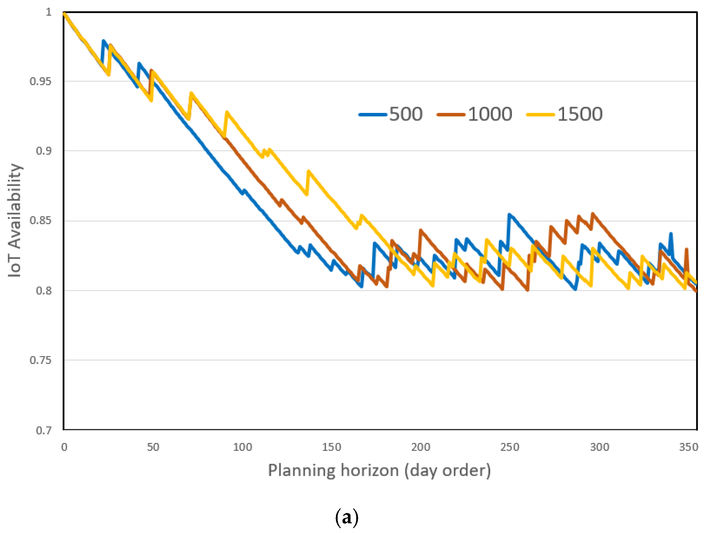
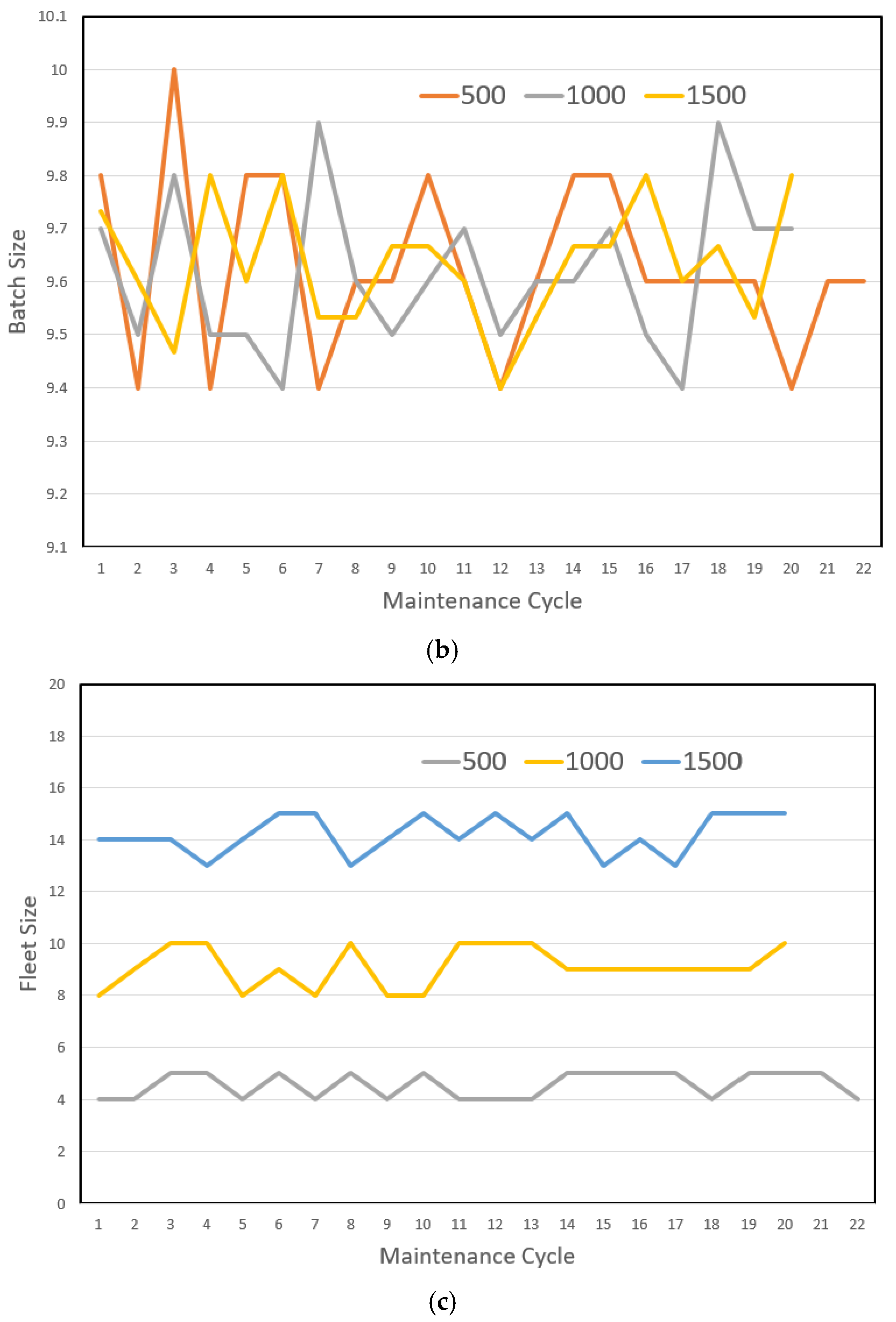
4.3. Scalability and Analysis

To test the scalability of the algorithms, the proposed heuristics and the GA were applied to each of the three datasets, IoT-500, IoT-1000, and IoT-1500. The numerical results were also analyzed to determine the properties of the maintenance programming model.

Table 4. Statistics of the model variables for the three IoT datasets.

	J	${\mathit{C}}_1$ Max Mean Min	${\mathit{D}}_{\mathit{p}\mathit{a}\mathit{t}\mathit{h}}$ Max Mean Min	${\mathit{C}\mathit{O}}_2$ Max Mean Min Threshold	${\mathit{L}}_{\mathit{j},\mathit{v}}$ Max Mean Min Threshold	$\widehat{\mathcal{R}}$ Max Mean Min Threshold	V Max Mean Min Threshold
IoT-500	22	6233 3898 2920	433.9 391.0 338.9	0.19 0.17 0.14 0.40	4.6 4.3 3.9 8.0	99.8% 85.7% 80.0% 80.0%	5.0 4.5 4.0 5.0
IoT-1000	20	8663 7555 6866	867.0 810.3 732.1	0.39 0.33 0.31 0.80	5.3 5.0 4.5 8.0	99.8% 86.3% 80.0% 80.0%	10.0 9.1 8.0 10.0
IoT-1500	20	16,006 14,527 13,487	1287.7 1203.3 1079.1	0.85 0.76 0.67 1.20	7.2 6.6 6.0 8.0	99.8% 86.6% 80.1% 80.0%	15.0 14.2 13.0 15.0

shows the resulting statistics obtained for the model variables. The numerical results offer several insights into the maintenance programming model. First, the number of required maintenance cycles for each dataset is similar. There are 22 maintenance cycles programmed for IoT-500 and 20 cycles for both IoT-1000 and IoT-1500. This is due to the fact that we set the fleet size to 5, 10, and 15 vehicles, which were proportional to the number of the microsites contained in the corresponding datasets, and the mean number of GA-determining on-duty vehicles V, as seen in the last column in Table 4, nearly reaches the fleet size. The mean time between two consecutive maintenance cycles estimated by 365 days/J for the three datasets ranged from 16.59 to 18.25 days, which is sufficient for the contract company to allocate the required maintenance materials and personnel. It is interesting to note that the time between early maintenance cycles is generally longer than that between later maintenance cycles. This is explainable by observing the historical IoT-normalized availability ($\widehat{\mathcal{R}}$), as shown in Figure 13a. The reliability of the microsites is 100% on their deployment day and then gradually declines during the following operation days. Some early-deployed microsites will need to be maintained earlier, but their reliability may not be restored to their as-new state, which is known as imperfect maintenance in the literature [33]. As more microsites are maintained, the IoT-normalized availability will be sustained within a small interval above the specified QoS lower bound (which was set to 80% in all our experiments), and more frequent maintenance cycles will need to take place in this period because of the aging and imperfect maintenance of the microsites. As seen in Figure 13a, the IoT-normalized availability for the three datasets remained within approximately 0.80 to 0.85 after 170 days during the planning horizon, and maintenance cycles were more frequently performed in this period. The mean IoT-normalized availability for the three datasets across the overall planning horizon was 85.7%, 86.3%, and 86.6%, as seen in Table 4, which is acceptable for an 80% QoS guarantee in terms of air quality monitoring IoT service availability.

The maintenance cost ($C_1$) spent on each cycle depends on the number of microsites (batch size) visited by each engineering vehicle and the types of maintenance activities performed. The mean batch size visited by each engineering vehicle in each maintenance cycle is shown in Figure 13b. It shows no significant difference in the mean batch size, which is between 9.4 and 10 for the three datasets. Because the mean number of GA-determining vehicles V listed in Table 4 is 4.5, 9.1, and 14.2 for the three datasets, the total number of maintained microsites in each cycle is around 40, 90, and 140, respectively. The ratio between these numbers is similar to that between the dataset sizes and that between the incurred mean maintenance costs ($C_1$), as shown in Table 4. The slight difference between the ratios is due to the probabilistic selection of one of the three types of maintenance activities. Moreover, the transportation cost ($C_2$), as calculated by Equation (18), is determined by the traveling distance ($D_{path}$) and the fuel efficiency (${\phi }_v$) of the on-duty vehicles. As the proposed GA employed almost all available vehicles in each cycle, the traveling distance became the dominant factor in the incurred transportation cost. Table 4 shows that the mean traveling distance for the three datasets is 391.0, 810.3, and 1203.3 km; the ratio between the distances is 1:2.07:3.08, which grows quasi-linearly with the number of microsites, i.e., 500, 1000, and 1500. This represents a good result for GA optimization in terms of finding the shortest routes, because the vehicle routing distance generally grows in a quadratic relationship with the number of visited sites.

Similarly, the CO₂ emissions (${CO}_2$), as calculated by Equation (20), are determined by the $D_{path}$ and ${\phi }_v$ of the performed vehicle. Since almost all available vehicles are used in every cycle by the GA, $D_{path}$ most influences the CO₂ emissions. To perform a sensitivity analysis, the CO₂ emissions limit was set to 0.4, 0.8, and 1.2 for the IoTs with 500, 1000, and 1500 microsites, respectively. It can be seen in Table 4 that the mean CO₂ emissions were 0.17, 0.33, and 0.76 tons, which were all well within the corresponding limits. Considering the worst case, the maximum CO₂ emissions amounted to 0.19, 0.39, and 0.85 tons, which were all significantly lower than the specified emission limits. These findings confirmed that the value for the CO₂ emissions limit should be linearly proportional to the number of microsites contained in the IoT.

The proposed GA approach tends to use up to the maximum number of vehicles in the fleet in every maintenance cycle, as shown in Figure 13c. This programming result is attributed to the constraint (23) on the maximum allowable working hours for labor associated with each vehicle. The actual maximum labor working hour values ($\underset{j,v}{\mathit{max}}{L}_{j,v}$) in each cycle are 4.6, 5.3, and 7.2, which are all less than the specified 8 h limit, conforming to the current requirements of the Taiwan Labor Standards Act.

5. Conclusions

In this paper, we have proposed a novel maintenance programming model for an outdoor IoT providing air quality monitoring services. Our task scenario significantly differs from classic maintenance programming in several aspects. Firstly, the maintenance of the IoT cannot be performed on an individual basis because the IoT connects a great number of microsites distributed across a large geographical area. We proposed heuristics to conduct batch maintenance and the scheduling of the batches. A GA was then designed to find the shortest routes by which to visit the batch microsites by a fleet of vehicles. Secondly, microsite failures will not cause the immediate breakdown of the air quality monitoring IoT but degrade the service quality to some extent. We defined a new measure, namely the IoT-normalized availability, to describe the confidence with which an IoT can provide air quality monitoring for a specified outdoor area. Thirdly, our vehicle routing programming is labor-friendly and air quality-friendly. The labor working hours per day, including the vehicle traveling time and maintenance performance time, should be confined within a maximum number according to the Taiwan Labor Standards Act. The total CO₂ emissions from the traveling vehicles also needs to be below a certain threshold to conform to our sustainability goal of clean air. Finally, our maintenance programming model searches for the minimum maintenance and transportation costs under hard constraints on the IoT-normalized availability, labor working hours, and CO₂ emissions. Simulations with our model were conducted using the government’s open data on the Central Taiwan air quality district, which contains an IoT with more than 1500 microsites. We produced three datasets from the IoT that included 500, 1000, and 1500 microsites to test the scalability of the proposed algorithms. The experimental results have the following implications. Firstly, the number of scheduled maintenance cycles remains near-constant if the fleet size grows linearly with the dataset size. Our simulation showed that the number of cycles was between 20 and 22 for all datasets, which implies that the mean time between two consecutive cycles is around 17 days, which is reasonably sufficient for the preparation of the required maintenance materials and personnel. Secondly, from the beginning of the planning time horizon, the IoT-normalized availability gradually deteriorated and finally fluctuated within a small interval above the specified IoT availability level. This is a good equilibrium between the cost and the QoS guarantee. Thirdly, the mean batch size (the number of microsites visited by an on-duty vehicle) in every maintenance cycle also remains near-constant. In our simulation, we found no significant difference in the mean batch size, which was between 9.4 and 10 for the three datasets. Moreover, the numerical results showed that the mean total vehicle traveling distance grew linearly with the fleet size. This leads to the desirable properties of our model, namely that the incurred mean maintenance cost and the mean transportation cost both grow linearly with the fleet size. This allows the decision-maker to deal with hard-constrained programming by focusing on controlling the fleet size in a linear relation to the number of microsites such that the allocation of resources, including budget, maintenance materials, and engineer personnel, is more easily managed.

There are some challenges for the future improvement of the proposed model and algorithms. The actual time spent in routing and maintenance may be longer than that estimated by the system due to traffic jams or work delays, which may lead to the violation of the maximum labor hours allowed in one day. The proposed system was installed on a smartphone, whose GPS could realize the real-time location of the vehicle and compare it to the expected location from the planned schedule. If any possible delay is large enough to lead to overdue work, a self-tuning heuristic should be activated to reroute the remaining tours of the nearest vehicles in order to share the microsite maintenance load and avoid overdue work.

References

1. Hwang, S.-L.; Lin, Y.-C.; Guo, S.-E.; Chi, M.-C.; Chou, C.-T.; Lin, C.-M. Emergency room visits for respiratory diseases associated with ambient fine particulate matter in Taiwan in 2012: A population-based study. Atmos. Pollut. Res. 2017, 8, 465–473. [Google Scholar] [CrossRef]
2. Song, C.; He, J.; Wu, L.; Jin, T.; Chen, X.; Li, R.; Ren, P.; Zhang, L.; Mao, H. Health burden attributable to ambient PM2.5 in China. Environ. Pollut. 2017, 223, 575–586. [Google Scholar] [CrossRef]
3. Chen, Y.-C.; Chiang, H.-C.; Hsu, C.-Y.; Yang, T.-T.; Lin, T.-Y.; Chen, M.-J.; Chen, N.-T.; Wu, Y.-S. Ambient PM2.5-bound polycyclic aromatic hydrocarbons (PAHs) in Changhua County, central Taiwan: Seasonal variation, source apportionment and cancer risk assessment. Environ. Pollut. 2016, 218, 372–382. [Google Scholar] [CrossRef]
4. Yin, P.-Y.; Tsai, C.-C.; Day, R.-F.; Tung, C.-Y.; Bhanu, B. Ensemble learning of model hyperparameters and spatiotemporal data for calibration of low-cost PM2.5 sensors. Math. Biosci. Eng. 2019, 16, 6858–6873. [Google Scholar] [CrossRef] [PubMed]
5. Yin, P.-Y.; Day, R.-F.; Lin, Y.-C.; Hu, C.-Y. Improving PM2.5 concentration forecast with the identification of temperature inversion. Appl. Sci. 2022, 12, 71. [Google Scholar] [CrossRef]
6. Yin, P.-Y.; Yen, A.-Y.; Chao, S.-E.; Day, R.-F.; Bhanu, B. A machine learning-based ensemble framework for forecasting PM2.5 concentrations in Puli, Taiwan. Appl. Sci. 2022, 12, 2484. [Google Scholar] [CrossRef]
7. Yin, P.-Y. A novel spatiotemporal analysis framework for air pollution episode association in Puli, Taiwan. Appl. Sci. 2023, 13, 5808. [Google Scholar] [CrossRef]
8. Lewis, A.; Peltier, W.-R.; von Schneidemesser, E. Low-Cost Sensors for the Measurement of Atmospheric Composition: Overview of Topic and Future Applications; Research Report; World Meteorological Organization: Geneva, Switzerland, 2018. [Google Scholar]
9. Yin, P.-Y. Mining associations between air quality and natural and anthropogenic factors. Sustainability 2024, 16, 4614. [Google Scholar] [CrossRef]
10. Elkateb, S.; Métwalli, A.; Shendy, A.; Abu-Elanien, A.E.B. Machine learning and IoT–based predictive maintenance approach for industrial applications. Alex. Eng. J. 2024, 88, 298–309. [Google Scholar] [CrossRef]
11. Toth, P.; Vigo, D. (Eds.) The Vehicle Routing Problem; Monographs on Discrete Mathematics and Applications; Society for Industrial and Applied Mathematics: Philadelphia, PA, USA, 2022; Volume 9, ISBN 0-89871-579-2. [Google Scholar]
12. Taiwan MOENV. Taiwan Air Quality Monitoring Network. Available online: https://airtw.moenv.gov.tw/CHT/EnvMonitoring/Central/spm.aspx (accessed on 15 February 2025).
13. Wang, Y.; Yang, W.; Han, B.; Zhang, W.; Chen, M.; Bai, Z. Gravimetric analysis for PM2.5 mass concentration based on year-round monitoring at an urban site in Beijing. J. Environ. Sci. 2016, 40, 154–160. [Google Scholar] [CrossRef]
14. Shukla, K.; Aggarwal, S.-G. A technical overview on beta-attenuation method for the monitoring of particulate matter in ambient air. Aerosol Air Qual. Res. 2022, 22, 220195. [Google Scholar] [CrossRef]
15. Day, R.-F.; Yin, P.-Y.; Huang, Y.-C.; Wang, C.-Y.; Tsai, C.-C.; Yu, C.-H. Concentration-temporal multilevel calibration of PM2.5 low-cost sensor. Sustainability 2022, 14, 10015. [Google Scholar] [CrossRef]
16. Basri, E.-I.; Abdul Razak, I.-H.; Ab-Samat, H.; Kamaruddin, S. Preventive maintenance (PM) planning: A review. J. Qual. Maint. Eng. 2017, 23, 114–143. [Google Scholar] [CrossRef]
17. Turner, C.-J.; Emmanouilidis, C.; Tomiyama, T.; Tiwari, A.; Roy, R. Intelligent decision support for maintenance: An overview and future trends. Int. J. Comput. Integr. Manuf. 2019, 32, 936–959. [Google Scholar] [CrossRef]
18. Camilotti, L.; Kurscheidt, R.; Loures, E.; Portela, E.; Freire, R. A review of maintenance scheduling methods in the context of Industry 4.0. In Proceedings of the 11th International Conference on Production Research—Americas. ICPR 2023; Deschamps, F., Pinheiro de Lima, E., Gouvêa da Costa, S.E.G., Trentin, M., Eds.; Springer: Cham, Switzerland, 2023. [Google Scholar] [CrossRef]
19. Sami, M.-A.; Khan, T.-A. Forecasting failure rate of IoT devices: A deep learning way to predictive maintenance. Comput. Electr. Eng. 2023, 110, 108829. [Google Scholar] [CrossRef]
20. Mijailovic, V. Probabilistic method for planning of maintenance activities of substation components. Electr. Power Syst. Res. 2003, 64, 53–58. [Google Scholar] [CrossRef]
21. Zhao, Y.-X. On preventive maintenance policy of a critical reliability level for system subject to degradation. Reliab. Eng. Syst. Saf. 2003, 79, 301–308. [Google Scholar] [CrossRef]
22. Nourelfath, M.; Nahas, N.; Ben-Daya, M. Integrated preventive maintenance and production decisions for imperfect processes. Reliab. Eng. Syst. Saf. 2016, 148, 21–31. [Google Scholar] [CrossRef]
23. Su, L.-H.; Tsai, H.-L. Flexible preventive maintenance planning for two parallel machines problem to minimize makespan. J. Qual. Maint. Eng. 2010, 16, 288–302. [Google Scholar] [CrossRef]
24. Tsai, Y.-T.; Wang, K.-S.; Teng, H.-Y. Optimizing preventive maintenance for mechanical components using genetic algorithms. Reliab. Eng. Syst. Saf. 2001, 74, 89–97. [Google Scholar] [CrossRef]
25. Van, P.-D.; Vu, H.-C.; Barros, A.; Berenguer, C. Grouping maintenance strategy with availability constraint under limited repairmen. IFAC Proc. 2012, 45, 486–491. [Google Scholar] [CrossRef]
26. Mahadevan, M.-L.; Poorana, K.-S.; Vinodh, R.; Paul, R.-T. Preventive maintenance optimization of critical equipment in process plant using heuristic algorithms. In Proceedings of the 2010 International Conference on Industrial Engineering and Operations Management, Dhaka, Bangladesh, 9–10 January 2010. [Google Scholar]
27. Samrout, M.; Yalaoui, F.; Chatelet, E.; Chebbo, N. New methods to minimize the preventive maintenance cost of series–parallel systems using ant colony optimization. Reliab. Eng. Syst. Saf. 2005, 89, 346–354. [Google Scholar] [CrossRef]
28. Adhikary, D.-D.; Bose, G.-K.; Jana, D.-K.; Bose, D.; Mitra, S. Availability and cost-centered preventive maintenance scheduling of continuous operating series systems using multi-objective genetic algorithm: A case study. Qual. Eng. 2016, 28, 352–357. [Google Scholar] [CrossRef]
29. Wang, S.; Liu, M. Multi-objective optimization of parallel machine scheduling integrated with multi-resources preventive maintenance planning. J. Manuf. Syst. 2015, 37, 182–192. [Google Scholar] [CrossRef]
30. Alabdulkarim, A.-A.; Ball, P.-D.; Tiwari, A. Applications of simulation in maintenance research. World J. Model. Simul. 2013, 9, 14–37. [Google Scholar]
31. Ab-Samat, H.; Jeikumar, L.-N.; Basri, E.-I.; Harun, N.-A.; Kamaruddin, S. Effective preventive maintenance scheduling: A case study. In Proceedings of the 2012 International Conference on Industrial Engineering and Operations Management, Istanbul, Turkey, 3–6 July 2012; pp. 1249–1257. [Google Scholar]
32. Shatz, S.-M.; Wang, J.-P.; Goto, M. Task allocation for maximizing reliability of distributed computer systems. IEEE Trans. Comput. 1992, 41, 1156–1168. [Google Scholar] [CrossRef]
33. Bhardwaj, S.; Bhardwaj, N.; Kumar, V.; Parashar, B. Imperfect maintenance modeling for sequential corrective and preventive maintenance. AIP Conf. Proc. 2022, 2357, 080006. [Google Scholar] [CrossRef]
34. Eiben, A.-E.; Smith, J.-E. Recombination for permutation representation. In Introduction to Evolutionary Computing, 2nd ed.; Natural Computing Series; Springer: Berlin/Heidelberg, Germany, 2015; pp. 70–74. [Google Scholar] [CrossRef]
35. Buontempo, F. Genetic Algorithms and Machine Learning for Programmers: Create AI Models and Evolve Solutions, Pragmatic Works Inc Programmers; Pragmatic Bookshelf: Raleigh, NC, USA, 2019. [Google Scholar]
36. Chen, L.-J.; Ho, Y.-H.; Lee, H.-C.; Wu, H.-C.; Liu, H.-M.; Hsieh, H.-H.; Huang, Y.-T.; Lung, S.-C. An open framework for participatory PM2.5 monitoring in smart cities. IEEE Access 2017, 5, 14441–14454. [Google Scholar] [CrossRef]
Figure 1. Taiwan air quality monitoring supersites and microsites deployed as of end of 2024. (a) Seventy-eight government-built supersites (image from https://airtw.moenv.gov.tw/ENG/default.aspx). (b) More than 10,000 participatory microsites (image from https://wot.moenv.gov.tw/). The watermark in the image states that the air quality measurements reported by the microsites are easily affected by local sources and do not reflect the air quality of large regions.
Sustainability 17 06522 g001
Figure 2. Microsite IoT in the Central Taiwan air quality district (image from https://wot.moenv.gov.tw/).
Sustainability 17 06522 g002
Figure 3. A typical microsite, which contains several types of sensors and ancillary devices mounted on a pole.
Sustainability 17 06522 g003
Figure 4. Reliability variations of sk with three maintenance cycles.
Sustainability 17 06522 g004
Figure 5. A heatmap visualizing the monitoring coverage area and the reliability of multiple microsites located at different locations.
Sustainability 17 06522 g005
Figure 6. An illustration of two neighboring microsites si and sj with overlapping effective monitoring coverage.
Sustainability 17 06522 g006
Figure 7. The chromosome coding scheme for the maintenance vehicle routing problem.
Sustainability 17 06522 g007
Figure 8. An illustrative example of PMX crossover. (a) Two parent chromosomes before performing PMX crossover; (b) two offspring chromosomes obtained after performing PMX crossover.
Sustainability 17 06522 g008
Figure 9. An illustrative example of 2-swap mutation. (a) A chromosome before performing 2-swap mutation; (b) resulting chromosome obtained after performing 2-swap mutation.
Sustainability 17 06522 g009
Figure 10. An illustrative example of the dashboard’s main features. (a) The first-layer control panel. (b) The second-layer control panel. The black arrows in the map indicate the vehicle traversal sequence.
Sustainability 17 06522 g010
Figure 11. Three geographical regions of Central Taiwan air quality monitoring IoT (image from Taiwan EPA, https://wot.moenv.gov.tw/).
Sustainability 17 06522 g011
Figure 12. An illustrative example of maintenance programming with our app interface on an Android smartphone. (a) Maintenance programming formulation and the obtained result on the first cycle; (b) planned vehicle routes; (c) maintenance programming formulation and the obtained result on the twenty fourth cycle; (d) reliability curve of microsite 185; (e) historical maintenance records of microsite 185.
Sustainability 17 06522 g012
Figure 13. Variations in the model variables for the three IoT datasets. (a) historical IoT-normalized availability; (b) batch size determined on each maintenance cycle; (c) fleet size determined on each maintenance cycle.
Sustainability 17 06522 g013aSustainability 17 06522 g013b