Author Contributions
Conceptualization, D.O., D.C. and A.J.R.N.; methodology, D.O. and D.C.; software, D.O.; validation, D.O., D.C. and A.J.R.N.; formal analysis, D.O., D.C. and A.J.R.N.; investigation, D.O.; resources, A.J.R.N.; data curation, D.O.; writing—original draft preparation, D.O.; writing—review and editing, D.O., D.C. and A.J.R.N.; visualization, D.O.; supervision, D.C. and A.J.R.N.; project administration, A.J.R.N.; funding acquisition, A.J.R.N. All authors have read and agreed to the published version of the manuscript.
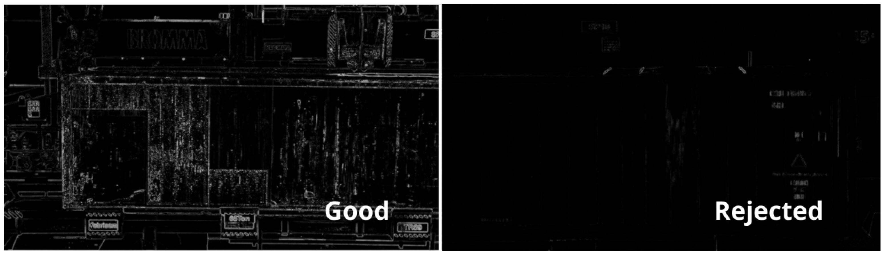
Figure 1.
Laplacian filter in selected and rejected examples.
Figure 1.
Laplacian filter in selected and rejected examples.
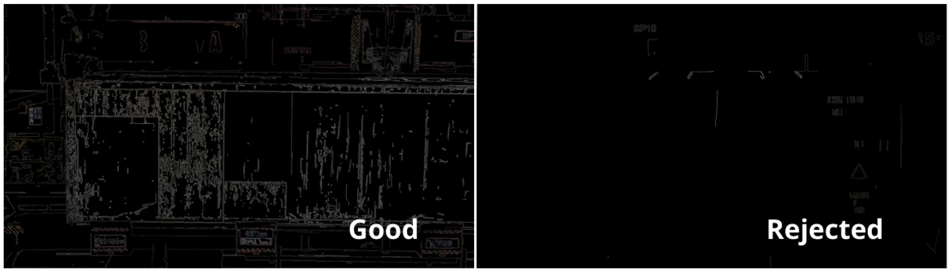
Figure 2.
Canny edge detection in selected and rejected examples.
Figure 2.
Canny edge detection in selected and rejected examples.
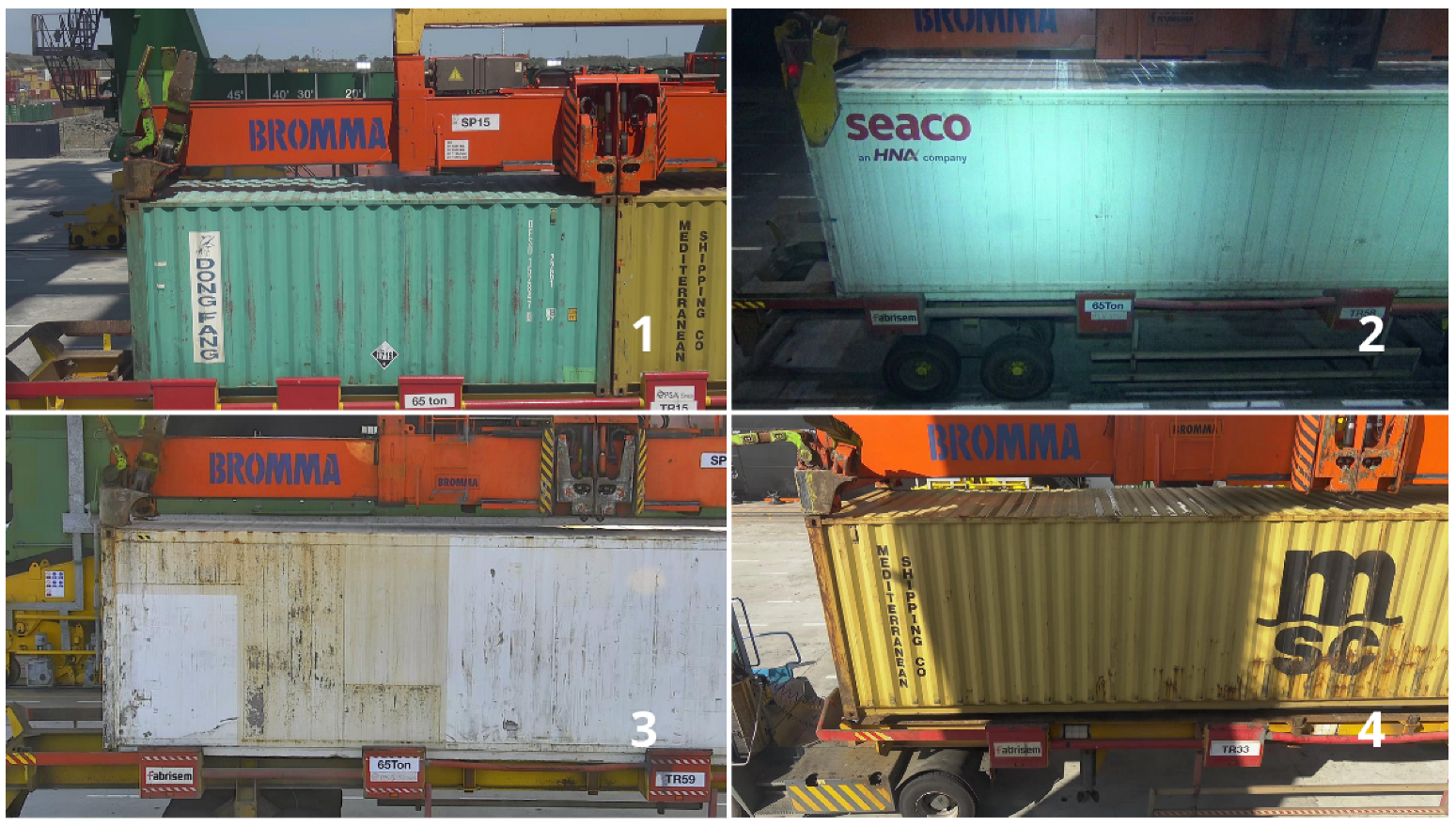
Figure 3.
Accepted images for the dataset, respecting the boundaries of the threshold blur (1–4).
Figure 3.
Accepted images for the dataset, respecting the boundaries of the threshold blur (1–4).
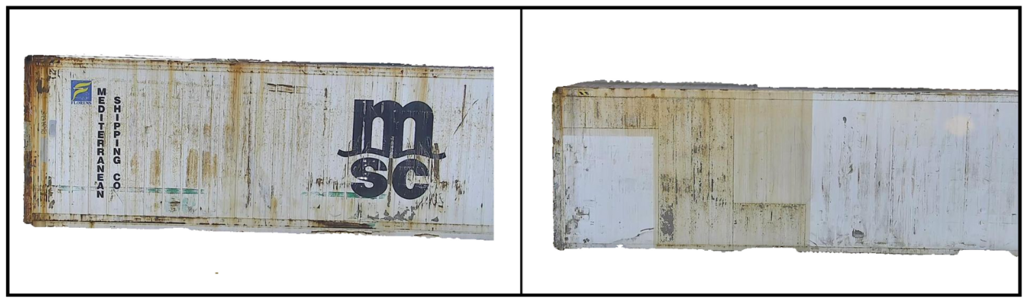
Figure 4.
Rejected images for dataset due to quality (1,2), blur (3), and brightness (4).
Figure 4.
Rejected images for dataset due to quality (1,2), blur (3), and brightness (4).
Figure 5.
Example of a fully annotated container.
Figure 5.
Example of a fully annotated container.
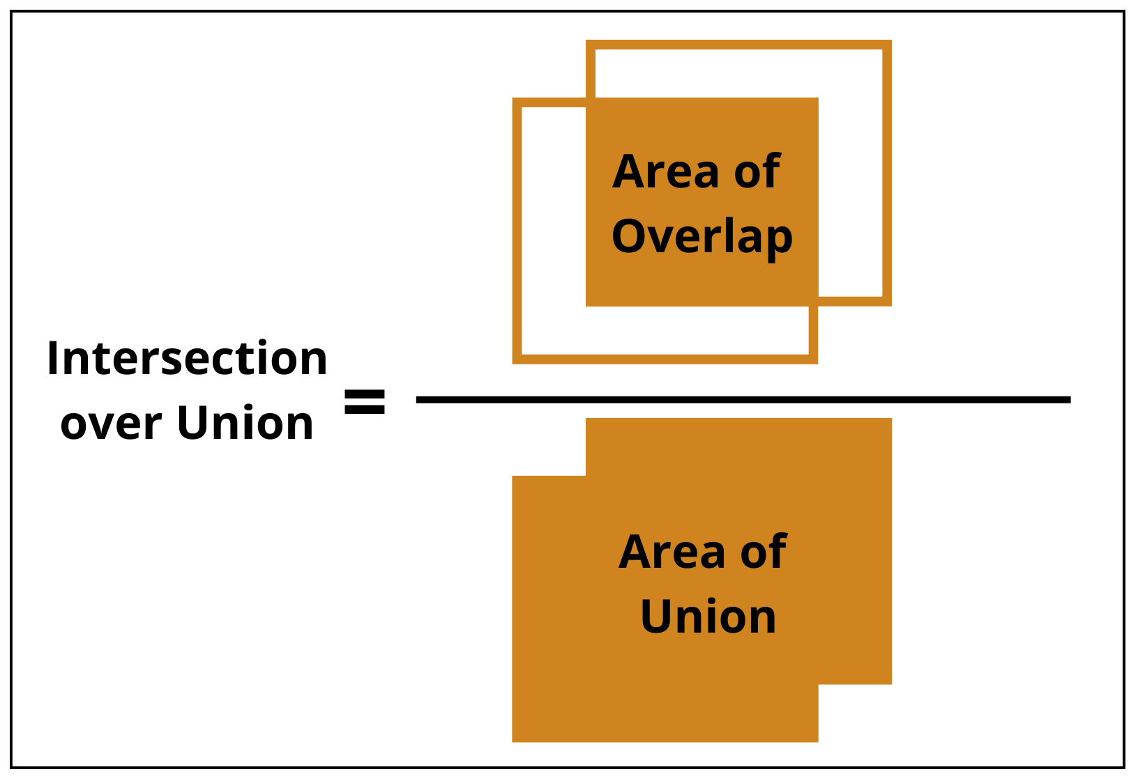
Figure 6.
Intersection over union metric.
Figure 6.
Intersection over union metric.
Figure 7.
Largest area segmented mask output from SAM.
Figure 7.
Largest area segmented mask output from SAM.
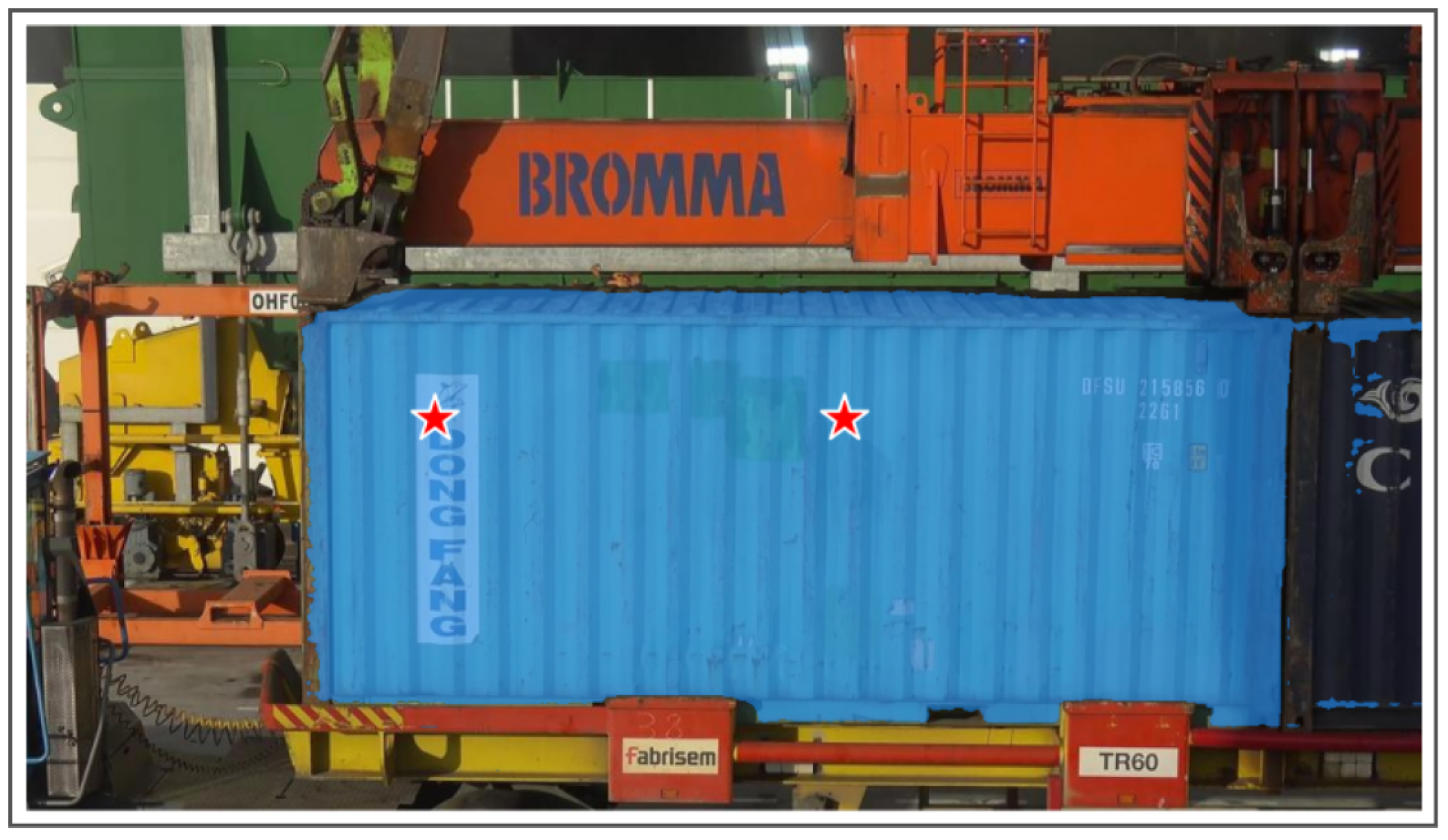
Figure 8.
Predictor output with 2 points (red star) as prompt. Best mask score: 0.975.
Figure 8.
Predictor output with 2 points (red star) as prompt. Best mask score: 0.975.
Figure 9.
Black and white background container masks.
Figure 9.
Black and white background container masks.
Figure 10.
Comparison of ground truth masks and model predictions for containers with distinct and similar corrosion colors.
Figure 10.
Comparison of ground truth masks and model predictions for containers with distinct and similar corrosion colors.
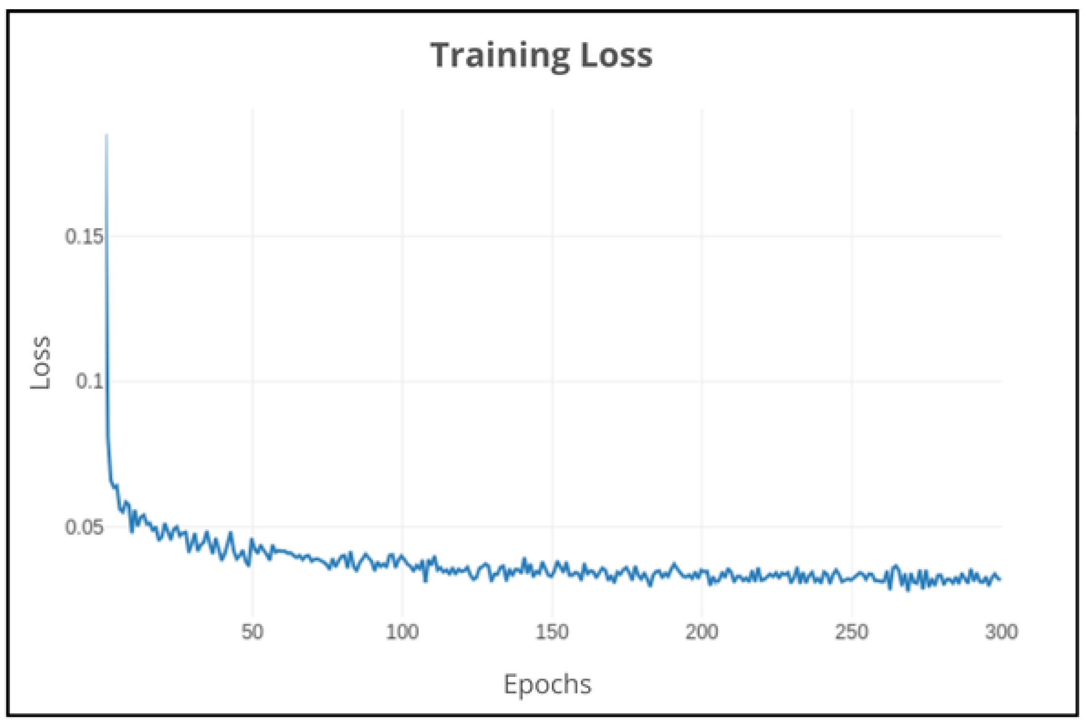
Figure 11.
DeepLabv3+: Training loss on 300 epochs using default parameters.
Figure 11.
DeepLabv3+: Training loss on 300 epochs using default parameters.
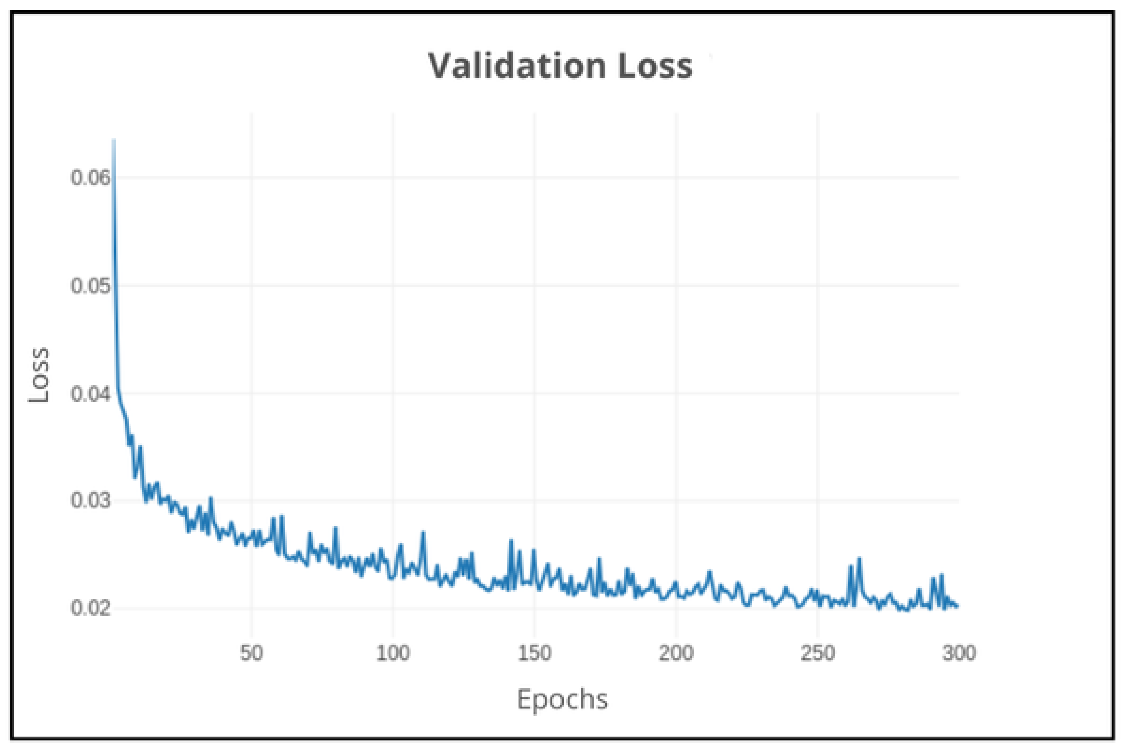
Figure 12.
DeepLabv3+: Validation loss on 300 epochs using default parameters.
Figure 12.
DeepLabv3+: Validation loss on 300 epochs using default parameters.
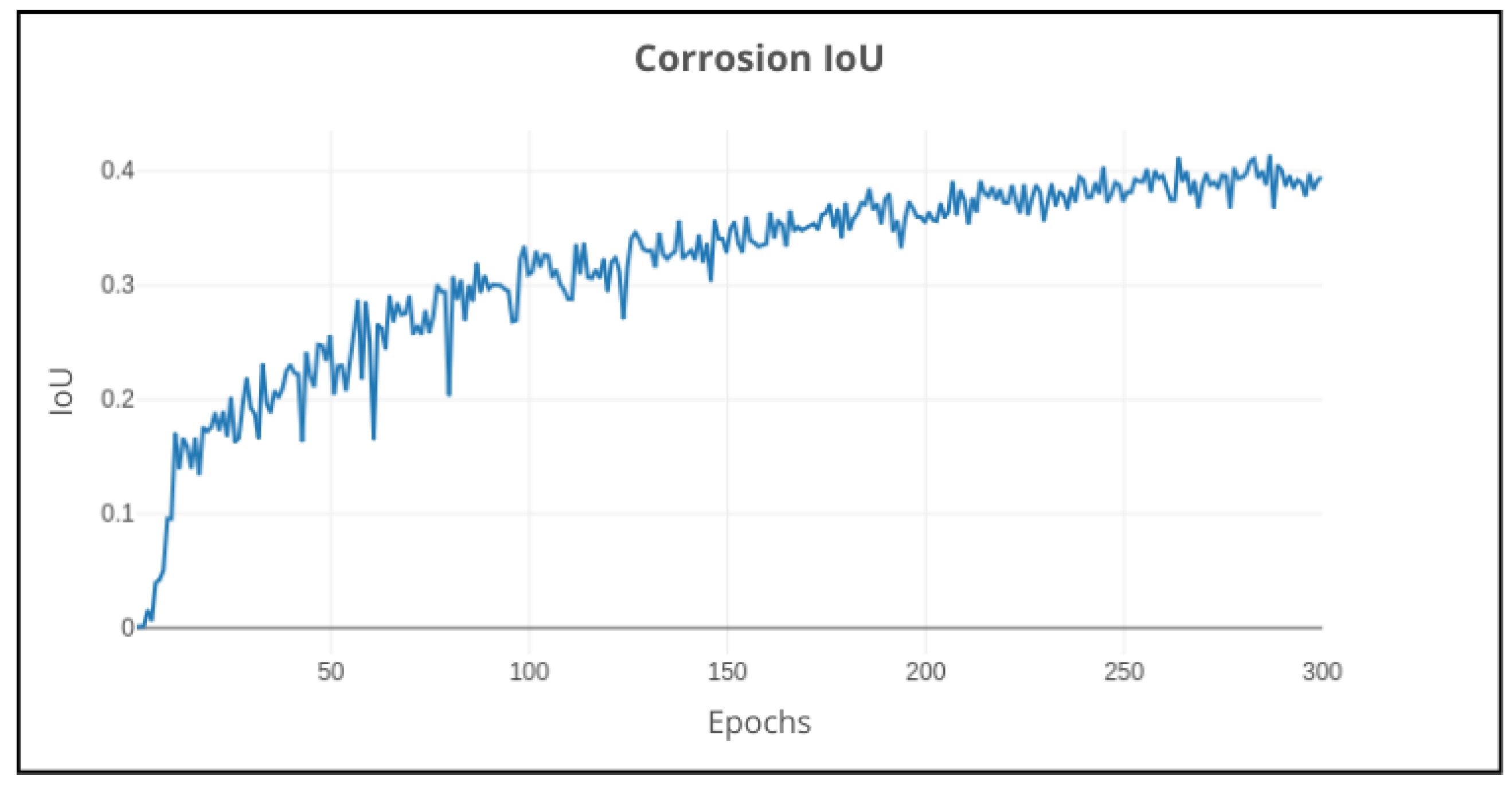
Figure 13.
DeepLabv3+: Validation performance of corrosion IoU on 300 epochs using default parameters.
Figure 13.
DeepLabv3+: Validation performance of corrosion IoU on 300 epochs using default parameters.
Figure 14.
DeepLabv3+ (bold lines: smoothed): Impact on validation performance using different backgrounds (default, white, and black) on 300 epochs.
Figure 14.
DeepLabv3+ (bold lines: smoothed): Impact on validation performance using different backgrounds (default, white, and black) on 300 epochs.
Figure 15.
DeepLabv3+: Impact on validation performance with or without data augmentation on 300 epochs.
Figure 15.
DeepLabv3+: Impact on validation performance with or without data augmentation on 300 epochs.
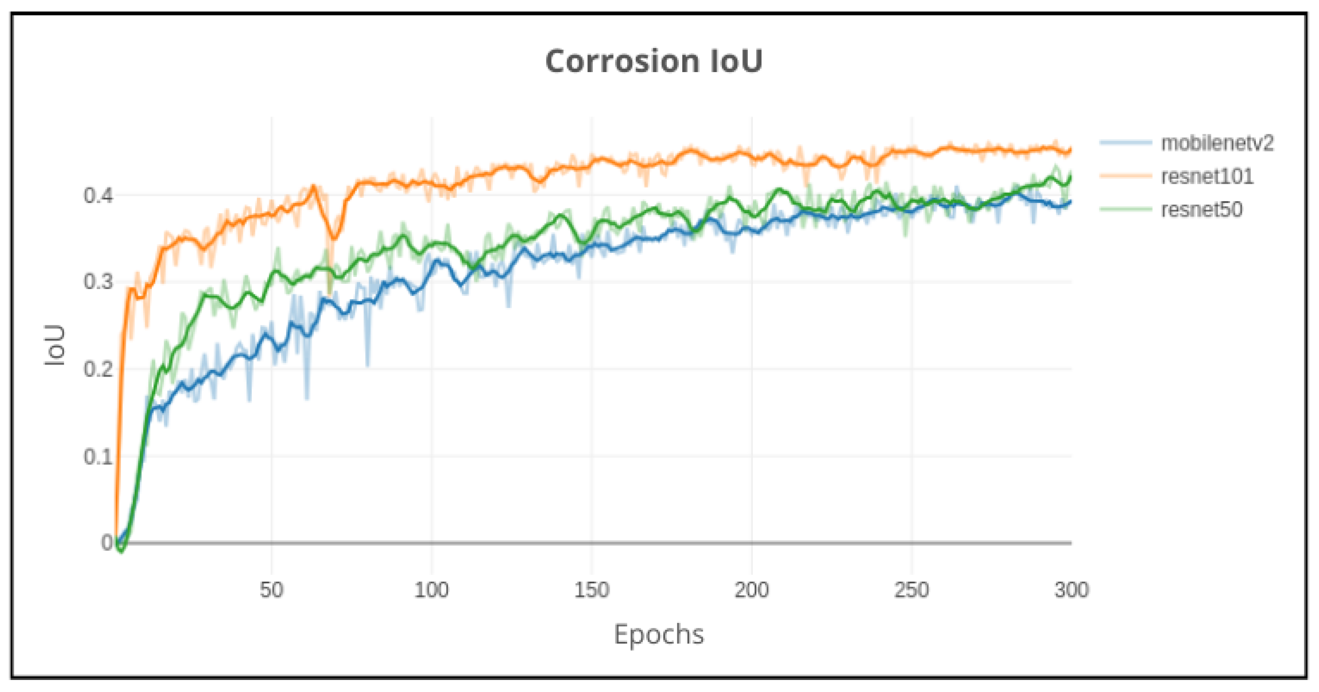
Figure 16.
DeepLabv3+ (bold lines: smoothed): Impact on validation performance using MobileNetv2, Resnet50, and Resnet101 backbone network models on 300 epochs.
Figure 16.
DeepLabv3+ (bold lines: smoothed): Impact on validation performance using MobileNetv2, Resnet50, and Resnet101 backbone network models on 300 epochs.
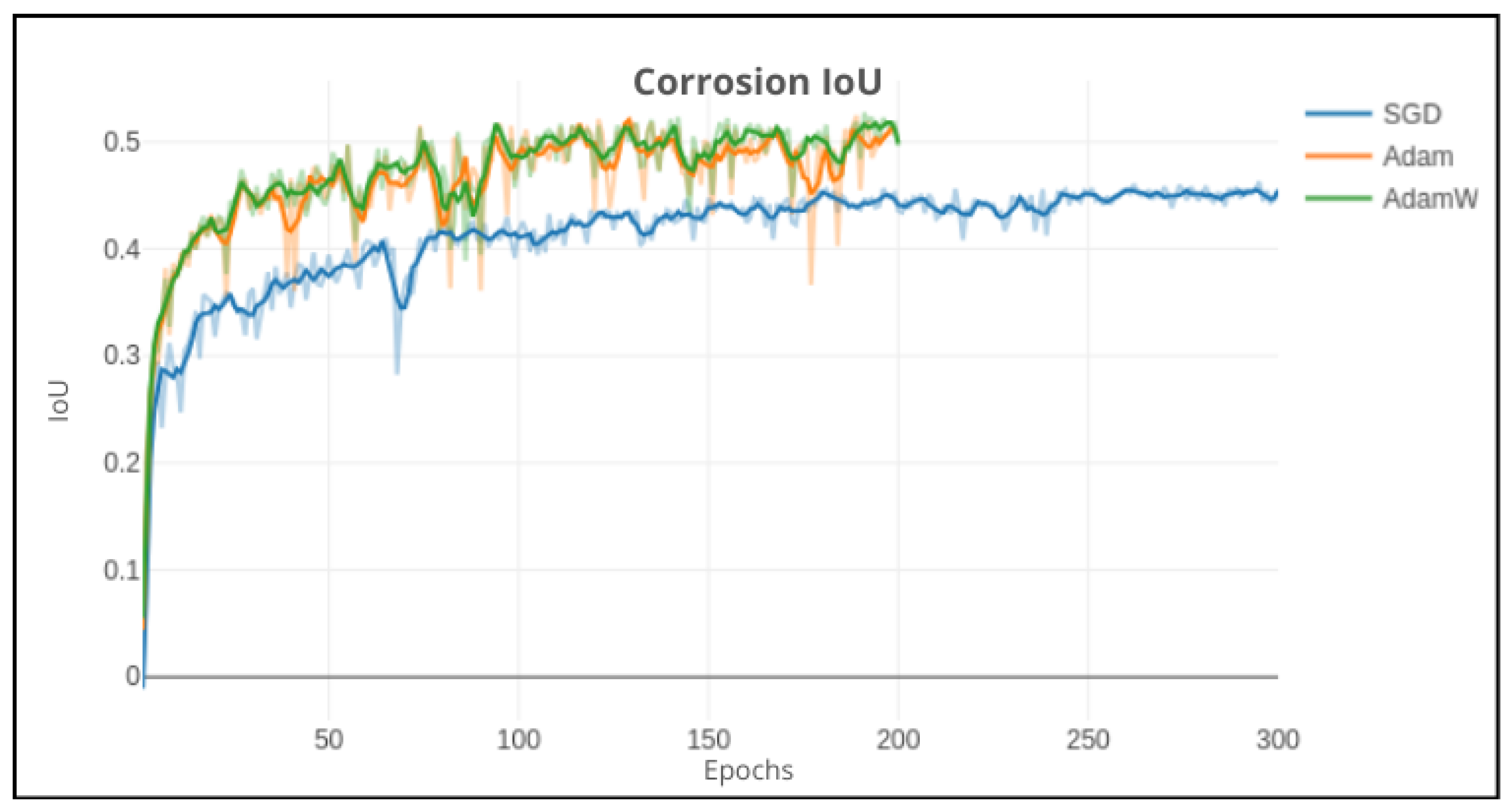
Figure 17.
DeepLabv3+ (bold lines: smoothed): Impact on validation performance using SGD on 300 epochs, Adam and AdamW on 200 epochs.
Figure 17.
DeepLabv3+ (bold lines: smoothed): Impact on validation performance using SGD on 300 epochs, Adam and AdamW on 200 epochs.
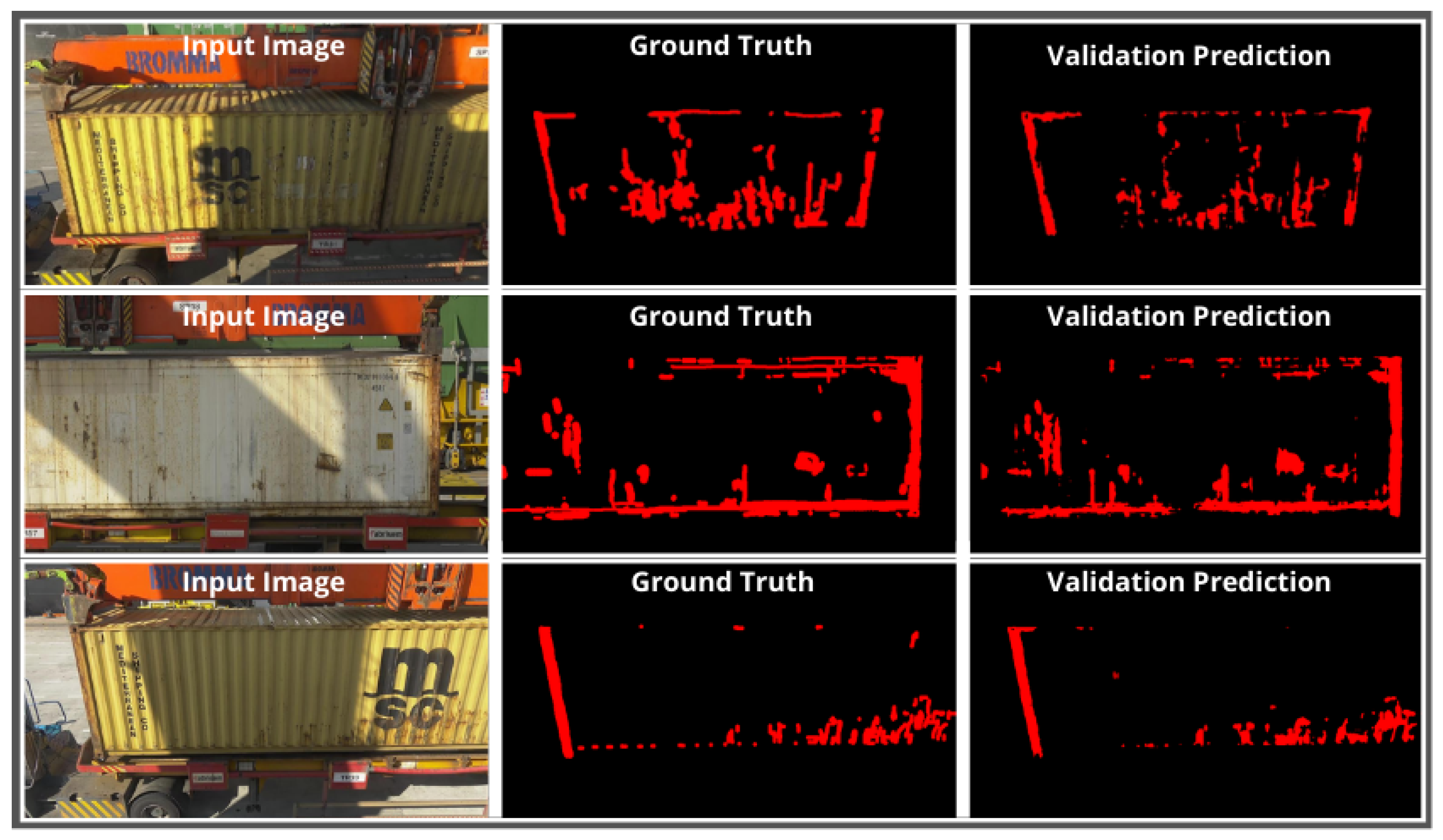
Figure 18.
Validation: Comparison of the output prediction with the ground truth mask and the original image.
Figure 18.
Validation: Comparison of the output prediction with the ground truth mask and the original image.
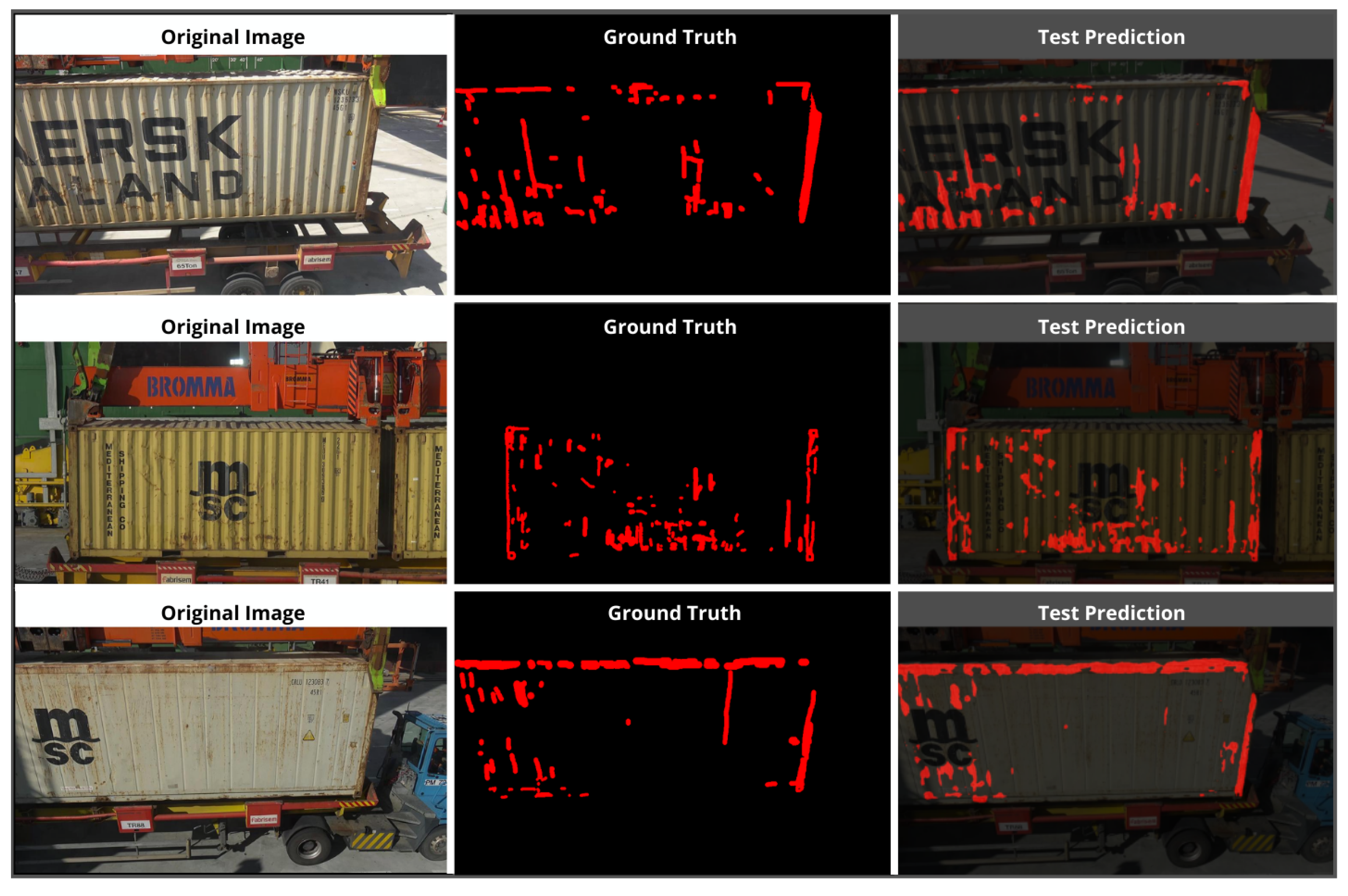
Figure 19.
Test: Comparison of the output prediction with the ground truth mask and the original image.
Figure 19.
Test: Comparison of the output prediction with the ground truth mask and the original image.
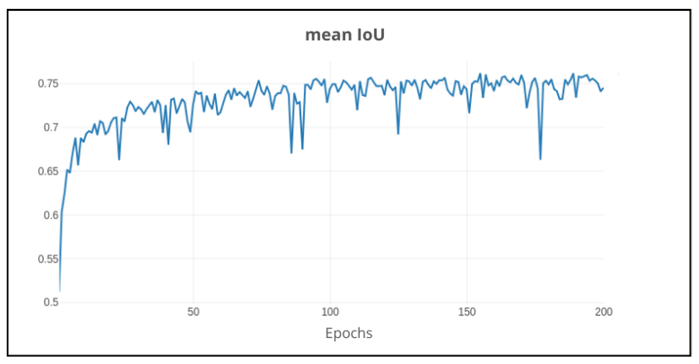
Figure 20.
Validation mean IoU using ResNet101 and AdamW (lr = 0.002) on 200 epochs.
Figure 20.
Validation mean IoU using ResNet101 and AdamW (lr = 0.002) on 200 epochs.
Figure 21.
CPU utilization during 60 s simulation using trained DeepLabv3+ as inference model.
Figure 21.
CPU utilization during 60 s simulation using trained DeepLabv3+ as inference model.
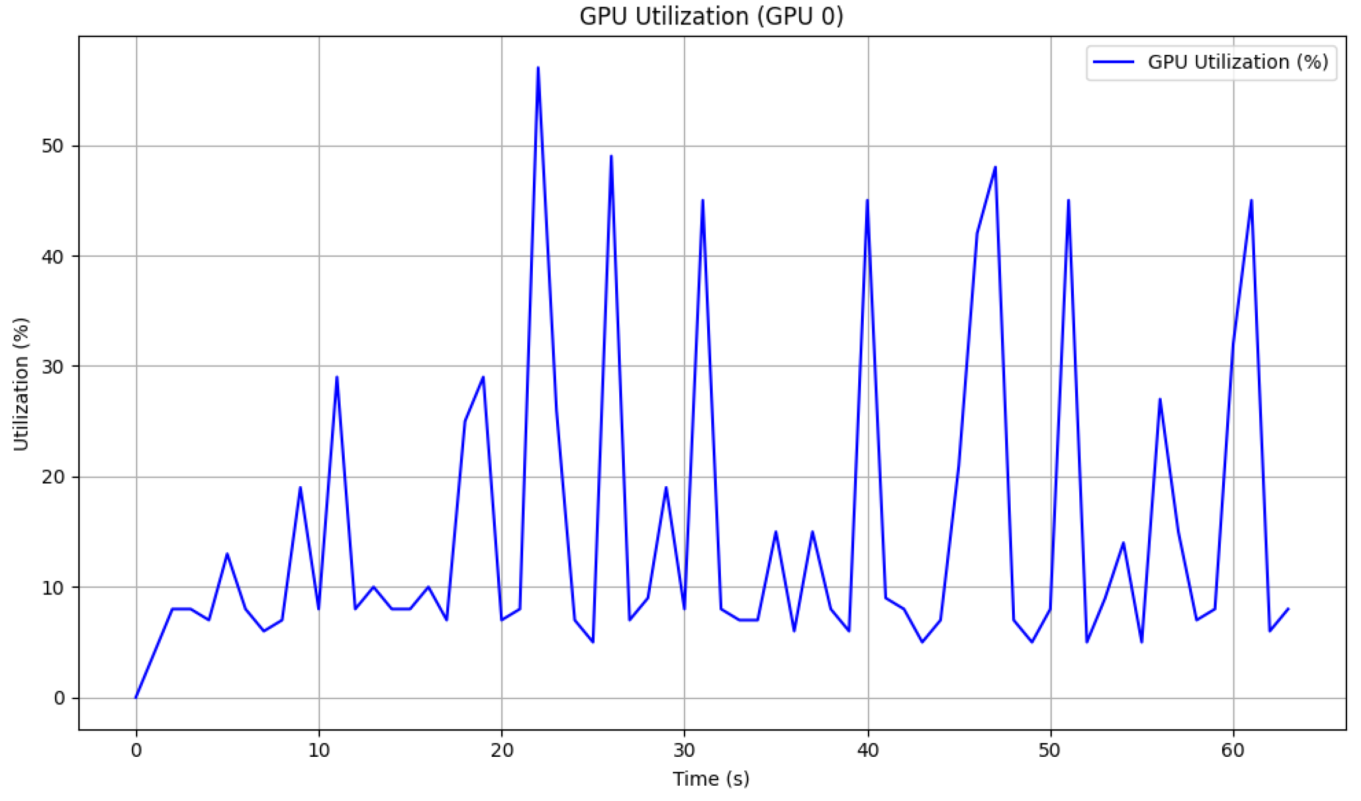
Figure 22.
GPU utilization during 60 s simulation using trained DeepLabv3+ as inference model.
Figure 22.
GPU utilization during 60 s simulation using trained DeepLabv3+ as inference model.
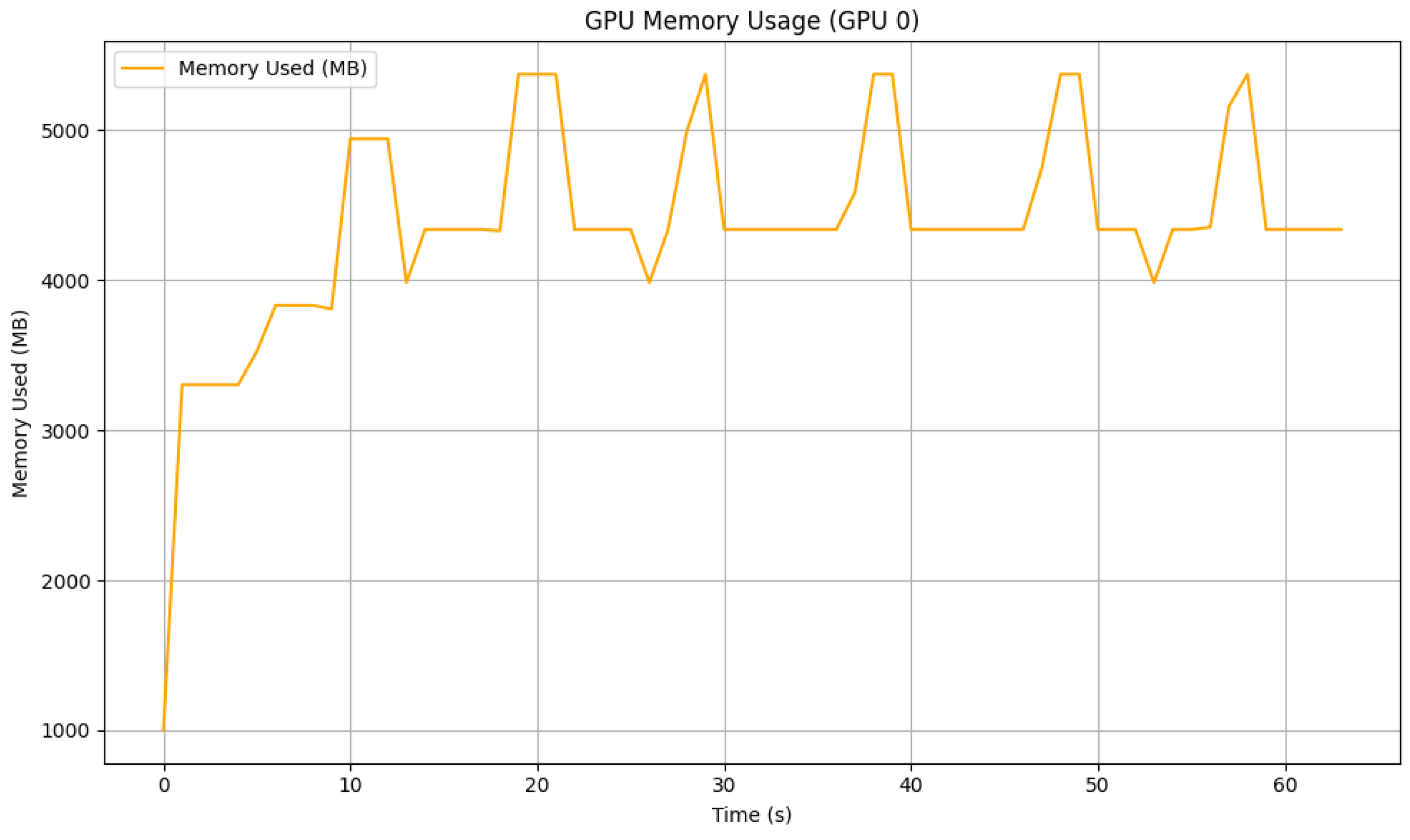
Figure 23.
GPU memory usage during 60 s simulation using trained DeepLabv3+ as inference model.
Figure 23.
GPU memory usage during 60 s simulation using trained DeepLabv3+ as inference model.
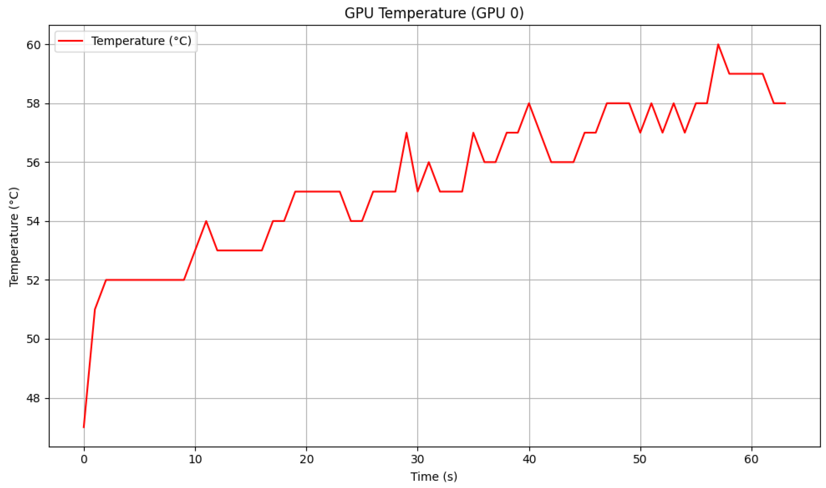
Figure 24.
GPU temperature during 60 s simulation using trained DeepLabv3+ as inference model.
Figure 24.
GPU temperature during 60 s simulation using trained DeepLabv3+ as inference model.
Table 1.
Number of canny edge pixels and Laplacian values.
Table 1.
Number of canny edge pixels and Laplacian values.
| Image | Canny Edges | Laplacian Variance |
|---|
| Rejected 1 | ≈77,000 | 11 |
| Rejected 2 | ≈42,000 | 11 |
| Rejected 3 | ≈6000 | 2 |
| Rejected 4 | ≈5500 | 3 |
| Accepted
1 | ≈316,000 | 54 |
| Accepted 2 | ≈129,000 | 23 |
| Accepted 3 | ≈137,000 | 85 |
| Accepted 4 | ≈318,000 | 50 |
Table 2.
Comparison of generic tools. (✓: Feature available, ✗: Feature not available).
Table 2.
Comparison of generic tools. (✓: Feature available, ✗: Feature not available).
| Tool | Open Source | Friendly UI | Large-Scale Datasets | Pixel-Level Labeling |
|---|
| CVAT | ✓ | ✓ | ✓ | ✓ |
| LabelStudio | ✓ | ✗ | ✓ | ✓ |
| LabelBox | ✓ | ✗ | ✓ | ✓ |
| VIA | ✓ | ✓ | ✗ | ✗ |
| LabelMe | ✓ | ✓ | ✗ | ✗ |
Table 3.
Comparison of CV annotation tools. (✓: Feature available, ✗: Feature not available).
Table 3.
Comparison of CV annotation tools. (✓: Feature available, ✗: Feature not available).
| Tool | Brush Tool | AI Magic Wand | Intelligent Scissors | Bounding Box | Points |
|---|
| CVAT | ✓ | ✓ | ✓ | ✓ | ✓ |
| LabelStudio | ✓ | ✓ | ✓ | ✓ | ✓ |
| LabelBox | ✓ | ✓ | ✓ | ✓ | ✓ |
| VIA | ✗ | ✗ | ✗ | ✓ | ✓ |
| LabelMe | ✗ | ✗ | ✗ | ✓ | ✓ |
Table 4.
Comparison of semantic segmentation models on PASCAL VOC 2012 dataset [
35].
Table 4.
Comparison of semantic segmentation models on PASCAL VOC 2012 dataset [
35].
| Model | mIoU % |
|---|
| FCN [36] | 67.2 |
| PSPNet [37] | 85.4 |
| SDN+ [38] | 86.6 |
| DeepLabV3-JFT [39] | 86.9 |
| DeepLabV3+ [23] | 89.0 |
Table 5.
DeepLabv3+ pre-trained performance (IoU) on experiments 1 (20 random images), 2 (40 images without red cargo containers), and 3 (20 images with only red cargo containers). The experiments were tested on all different model weights with each respective loss function: w18 (cross entropy), w27 (L1 loss), w35 (L2 loss), w40 (cross entropy with weighted classes). Comparison of model performance in original image against white and black backgrounds.
| Experiments | Weights | Original | White Background | Black Background |
|---|
| 1 | 18 | 9.3% | 14.5% | 16.3% |
| 27 | 15.5% | 20.4% | 21.1% |
| 35 | 14.9% | 18.7% | 18.9% |
| 40 | 10.3% | 22.0% | 20.5% |
| 2 | 18 | 6.9% | 13.1% | 14.9% |
| 27 | 12.2% | 17.7% | 18.5% |
| 35 | 9.2% | 14.4% | 14.9% |
| 40 | 9.3% | 18.3% | 14.8% |
| 3 | 18 | 0.6% | 1.4% | 1.6% |
| 27 | 0.9% | 2.4% | 1.9% |
| 35 | 1.0% | 1.5% | 1.5% |
| 40 | 0.8% | 0.9% | 1.7% |
Table 6.
DeepLabv3+ fine-tuned performance (IoU) on validation set and test set for each configuration in all experiments.
Table 6.
DeepLabv3+ fine-tuned performance (IoU) on validation set and test set for each configuration in all experiments.
| Experiments | Configuration | Validation | Test |
|---|
| Background | Default | 41.3% | 30.0% |
| Black | 40.1% | 30.4% |
| White | 41.0% | 29.5% |
| Data augmentation | Default | 41.3% | 30.0% |
| Without | 39.4% | 29.3% |
| Networks | MobileNetV2 (def) | 41.3% | 30.0% |
| ResNet50 | 43.2% | 34.7% |
| ResNet101 | 46.3% | 40.1% |
| Optimizers | SGD (def) | 46.3% | 40.1% |
| Adam | 52.5% | 49.4% |
| AdamW | 52.7% | 49.4% |
Table 7.
Performance comparison of DeepLabv3+ pre-trained model with fine-tuned model.
Table 7.
Performance comparison of DeepLabv3+ pre-trained model with fine-tuned model.
| DeepLabv3+ Model | Performance (IoU) |
|---|
| Pre-trained | 4.0% |
| Fine-tuned | 49.4% |


