Farm Greenhouse Gas Emissions as a Determinant of Sustainable Development in Agriculture—Methodological and Practical Approach

Abstract

Climate change is one of the most important environmental problems of the modern world. Without an effective solution to this problem, it is not possible to implement sustainable development. For this reason, in the European development strategies, including the European Green Deal (EGD), the reduction in greenhouse gas (GHG) emissions is one of the priorities. This also applies to sectoral strategies, including those related to agriculture. In this context, the monitoring of changes in GHG emissions becomes particularly important, and its key condition is an applicative estimation method, adapted to the available data and levels of assessment (globally, country, sector, economic unit). GHG emission calculations at the level of the agricultural sector are officially estimated by the state and non-governmental organisations. However, calculations at the level of the agricultural unit-farm remain a challenge due to the lack of detailed data or its incomplete scope to estimate GHG emissions. The other issue is the necessity of a representative data nature, taking into consideration the different profiles of various farms. The research focused on presenting a methodological approach to utilising FADN (Farm Accountancy Data Network) data for estimating GHG emissions at the farm level. The Intergovernmental Panel on Climate Change (IPCC) methodology was adopted to use available farm-level data. Some assumptions were needed to achieve this goal. The article presents the subsequent stages of GHG calculation using the FADN data. The results reveal significant differences in GHG emissions among farm types. The presented results indicated the primary sources of emissions from agriculture, including energy (e.g., fuel and electricity consumption), thus outlining the scope of action that should be taken to reduce emissions effectively. The study confirms that the method used helps estimate emissions at the farm level. Its application can lead to better targeting of climate policy in agriculture.

1. Introduction

Modern climate change is a phenomenon whose existence should not be in doubt [1,2]. It is evidenced by numerous long-term measurements observed in various parts of the world [3,4]. On this basis, we also know that it is a global phenomenon whose regional impact is not homogeneous, but in practice affects the entire planet [5,6]. The main factor of change is the concentration of greenhouse gases in the atmosphere, which varies globally. The effects of this phenomenon, such as long-term temperature changes and changes in water availability, can be felt differently, but they appear on all continents.

The causes of this phenomenon are also well understood [7,8,9,10], which enables scientists to unequivocally state that the current climate change is anthropogenic in nature [11,12,13]. This also means that its counteraction can only be achieved through human activity.

There should also be no discussion about the need to combat climate change, as extensive research and evidence demonstrate that the adverse effects of climate change outweigh the positive ones [14,15,16,17,18]. One may wonder how large the scale of these effects can be, but the trend itself is clearly shown [2].

Numerous observations indicate that we are facing rapid climate change, which has a global impact [3,19]. The magnitude of the effects caused by this process varies from region to region, but it is observed on the surface of the entire planet [20].

Forecasts [21,22,23,24,25] indicate that the problem of climate change will intensify and lead to numerous challenges for human civilisation [26]. These among others include the occurrence of a heat wave, problems with access to water, the increase in of adverse weather phenomena in greater quantity and intensity, droughts and fires, migrations of species, including carriers of diseases (affecting plants and animals, including humans), extinction of species and destruction of ecosystems, problems with access to food, rising costs of adapting to changing climate conditions, flooding of low-lying areas, migrations, etc.

The multitude of effects and the scale of impact on humans and the environment make climate change one of the most important problems that needs to be taken into account in sustainable development strategies. It can even be said that nowadays it is impossible to implement a sustainable development policy without taking into account the problem of climate change. The priority in this area is to reduce GHG emissions. The need to take climate change into account in sustainable development is visible both in the activities of the United Nations, e.g., in the 2030 Agenda [27], and in European Union documents, e.g., the European Green Deal (EGD) [28], including sectoral strategies, e.g., on agriculture, i.a., Farm to Fork [29] and Biodiversity Strategy [30].

The global nature of climate change necessitates a global solution to this problem. International cooperation and adoption of appropriate policies by the countries, the main emitters of greenhouse gases, is a necessary condition for success. At the same time, this does not mean that reduction measures are only taken at the international level. This is the level at which goals are set, for example, under the Paris Agreement, but their implementation falls to individual countries and entities operating within them.

So far, the political actions taken at the global level have not brought optimism. Both statistical data [31,32] and the evaluation of discussions held on the international forum indicate that the undertaken activities are not very effective [33,34]. The U.S. decision in January 2025 to withdraw from the Paris Agreement also resulted in a decline in interest in international action to combat climate change.

The exception is the actions of the European Union, which is leading the way in achieving climate neutrality by 2050. The main assumptions for achieving this goal are outlined in the EGD and also appear in earlier documents [35]. However, this requires a very detailed approach to climate policy.

The low effectiveness of climate policy has led to an increasingly urgent need to intensify action to mitigate climate change. This applies to all sectors of human activity, including agriculture [36].

Agriculture is one of the economic sectors that, on the one hand, is strongly dependent on climatic conditions [17,37,38,39,40,41,42,43,44], and on the other hand, is a significant emitter of greenhouse gases [45,46,47]. In the EU, almost 12% of GHG emissions are produced by this sector. In Poland, the share of emissions from agriculture is smaller (9.9%), but still significant (

Table 1. GHG emissions in the EU and Poland in 2022 (mln tonnes CO₂ eq/year).

Sector	EU 27	Poland
Agriculture	380.57	35.92
Buildings	455.96	47.92
Fuel Exploitation	197.81	27.20
Industrial Combustion	322.02	26.03
Power Industry	651.56	119.94
Processes	294.49	27.98
Transport	781.52	68.70
Waste	137.87	10.11
Total	3221.79	363.79

Source: own study based on EDGAR database [4].

). The implementation of the climate neutrality goal announced in the EGD and other documents requires decisive reduction measures in this sector as well. Without it, the real chances of achieving these goals are minimal, approaching zero. It is worth noting that agriculture is not only an emitter of greenhouse gases, but also contributes to their absorption. Carbon is one of the elements necessary for plant development. It is stored in them. Absorption is also related to the fixation of carbon in the soil. The number of removals depends on the type of crop and the agricultural practices used to farm the soil. For this reason, according to the Intergovernmental Panel on Climate Change (IPCC), these processes are not formally assigned to the agricultural sector, but to the LULUCF soil management sector. The National Centre for Emissions Management (KOBiZE) estimates the net effect of CO₂ absorption from agricultural soils at 1.06 million tonnes of CO₂ equivalent per year. This is a small part of the emissions caused by this sector, which makes efforts to reduce emissions in agriculture necessary.

This means that activities in this sector should be of particular interest; however, due to the reluctance to change, a lack of appropriate knowledge, limited investment funds, and the dispersed and heterogeneous nature of the issue, activities in this sector are progressing much slower than expected. This is particularly evident in the European Union, where in the second decade of the 21st century, simple reduction solutions began to run out. This led to a slowdown in the pace of emission reductions [45].

In this situation, there is a need to look for more detailed solutions to reduce GHG emissions, which would enable the transfer of national reduction targets to actions taken at the level of agricultural holdings. To do this, knowledge of emissions at the farm level is essential. Such knowledge will enable the determination of which farms will yield the best results from implementing climate policy.

Measuring GHG emissions at the farm level should be carried out using appropriate climate calculators. Their low use in climate policy is due to several limitations [48,49], including the lack of widespread use of tools, the multiplicity of tools on the market, and the differences in the method of calculating emissions between them, as well as the differences between the methodology of calculating emissions used in these calculators and in the state’s climate policy. Additionally, the lack of historical information on farm emissions remains a limitation.

For these reasons, it is more advisable to use very detailed statistical data that are available in a given country. In the European Union, FADN (Farm Accountancy Data Network) data can be used for this purpose.

This study aims to present differences in GHG emissions between types of farms in Poland. At the same time, our goal is to demonstrate the method for estimating emissions from a farm in Poland based on data from the FADN database. Similar actions have already been taken in both the European Union [50,51,52,53] and Poland [54,55,56,57]. However, in Poland, the method has never been presented in such detail, making it impossible to replicate previous studies, such as on current data. A factor that distinguishes this study from previous studies is the use of individual data from farms, along with a comprehensive presentation of the method, its advantages, challenges related to its application, and limitations.

A factor that distinguishes this study from others is the estimation of emissions at the farm level on a very large sample, i.e., 11,029 entities. In addition, the article presents the method of estimating emissions in detail, indicating not only the individual stages of this process but also the formulas and indicators used to obtain the results. This resulted in a significant expansion of the methodological part of the article, allowing subsequent users to replicate the research and assess its accuracy. In the case of many previous studies, only general methodological assumptions were given, which do not allow for the repetition of the research. Such a detailed presentation of the method adds significant value to this article. It also allows for showing methodology gaps and possibilities for future research. The results obtained, which show differences in emissions depending on the type of farm, as well as the number of animals and the Utilised Agricultural Area (UAA), should also be considered a novelty in research on GHG emissions in Polish agriculture.

2. Materials and Methods

2.1. About IPCC and KOBiZE—The Institution’s Significance

To calculate gas emissions at the farm level, the guidelines described by the Intergovernmental Panel on Climate Change (IPCC) were used. The IPCC was established by the United Nations Environment Programme (UNEP) and the World Meteorological Organisation (WMO) in 1988 to assess the state of knowledge on climate change and to establish international standards for climate change measurement. These are the most accurate methods of measuring emissions. This is also true for the agricultural sector as a whole, where emissions per country are calculated based on three basic levels of data granularity. The most general is Tier I, where emissions are calculated based on IPCC-specific indicators [58]. Data at this level comes from national or international databases. Tier II provides for the use of local data and global or national indicators, adapted to local conditions. Tier III is implemented using local data and indicators developed based on local surveys [59].

In Poland, emission estimates are prepared by the National Centre for Emissions Management—KOBiZE. In the case of agriculture, solutions from all three levels apply, i.e., Tier I, II, and III. This study uses the indicators used by KOBiZE in 2022, which correspond to the appropriate levels of data granularity. At the time of the research, these were the most up-to-date published indicators.

Based on the above sources, the emission estimation procedure was carried out using the diagram below (Figure 1). First, emissions from individual agricultural activities undertaken on the farm were calculated. This was the most challenging part of the work because it required the adoption of numerous assumptions related to adapting FADN data to the IPCC method used in Poland. This required estimating certain items, which we have clearly shown by presenting the calculation method in Section 2.4. The results were calculated in kilograms of greenhouse gases emitted, such as carbon dioxide (CO₂), methane (CH₄), and nitrous oxide (N₂O). Then, the emissions for individual gases were totalled. The next step was to calculate the average emissions per farm. This required reducing the emissions of individual greenhouse gases to a common denominator, i.e., carbon dioxide equivalent (CO₂ eq). The final stage of the work involved estimating emissions for different types of farms and highlighting the differences between them. Artificial intelligence technology was not used to carry out any stage of the work.

2.2. GHG Emissions from Agriculture vs. Agricultural Sector

Agriculture, and more specifically each farm, generates emissions that, according to the IPCC guidelines, are classified in the relevant part into three different emission sectors: Sector 1—Energy, Sector 3—Agriculture, and Sector 5—Land Use, Land-Use Change, and Forestry (LULUCF). As a result of this methodology for calculating and qualifying emissions by individual sectors, many activities undertaken at the farm level may lead to changes in greenhouse gas emissions, which will not be reflected in the numerical reduction in emissions at the sector level (i.e., Sector 3). This is important from the perspective of the climate policy pursued and the use of appropriate tools to monitor changes in the impact of agriculture on the climate. The most striking example of this is measures related to reducing energy consumption on the farm, which are reflected in the emission account, but only in the energy sector. The use of more efficient equipment, practices that require less use of machinery, or thermal modernisation of buildings does not result in a reduction in emissions in the agricultural sector, although it contributes to the overall reduction in GHG emissions. The same is in the land-use sector. The conversion of arable land to pasture or perennial crops leads to emission reductions; however, such a change is attributed to a distinct sector of land-use change. Even some agricultural practices, e.g., no-tillage farming, are qualified in this way. This means that the number of reduction measures in the agricultural sector that can translate into a numerical result presenting gas reductions in agriculture is limited.

In practice, the measurement of emissions in the agricultural sector primarily involves analysing the 11 areas listed in

Table 2. Sources of GHG emissions in the agricultural sector according to the IPCC.

Lp.	Process	GHG Type
1.	Enteric Fermentation	CH4
2.	Manure Management	CH4, N2O
3.	Inorganic N fertiliser use	N2O
4.	Organic N fertilisers use animal manure and sewage sludge	N2O
5.	Urine and dung deposited by grazing animals	N2O
6.	Crop residues	N2O
7.	Mineralisation/immobilisation associated with loss/gain of soil organic matter	N2O
8.	Cultivation of organic soils (i.e., histosols)	N2O
9.	Indirect N2O emissions from managed soils	N2O
10.	Field Burning of Agricultural Residues	CH4, N2O
11.	CO2 emissions from liming, urea, and other carbon-content fertilisers use	CO2

Source: own study based on KOBiZE [60].

.

2.3. Farm’s Level Data—The Key Issue—FADN Significance

Data from the Polish FADN database were used to assess greenhouse gas emissions at the farm level. FADN is the European system for collecting accounting data from agricultural holdings. On average, FADN data in Poland are collected from approximately 11,000 farms.

The specificity of FADN means that not all data necessary for full emission determination are available. Basic data such as the size of the livestock, the sown area or the size of the harvest, as well as information on the amount and type of mineral fertilisation, are available; however, data on fertilisation with natural fertilisers or agricultural practices are not collected. Natural fertilisation can be estimated based on the size of the livestock population, which was used in this study. Estimations concerned with energy use in quantitative terms. Energy consumption was estimated based on cost data available in FADN sources. As a result, it is necessary to use indirect methods to obtain other relevant data and estimate emissions on this basis. Nevertheless, FADN data seem to be the most suitable for this purpose, due to the unified system of data collection in individual EU Member States, their annual collection, and their representativeness for the population of commercial farms in a given country, taking into account the size and type of agricultural farms.

In the FADN database, there are commercial farms with a Standard Output of at least 4000 euros. This means that most farms in Poland are not represented in this database, due to their small-scale production; thus, the FADN data are not representative of the entire sector. This also makes it impossible to compare them with the emission data estimated and published by KOBiZE, which applies to the entire agricultural sector. Nevertheless, commodity farming, due to its large-scale production, has a significant impact on the volume of emissions from the agricultural sector.

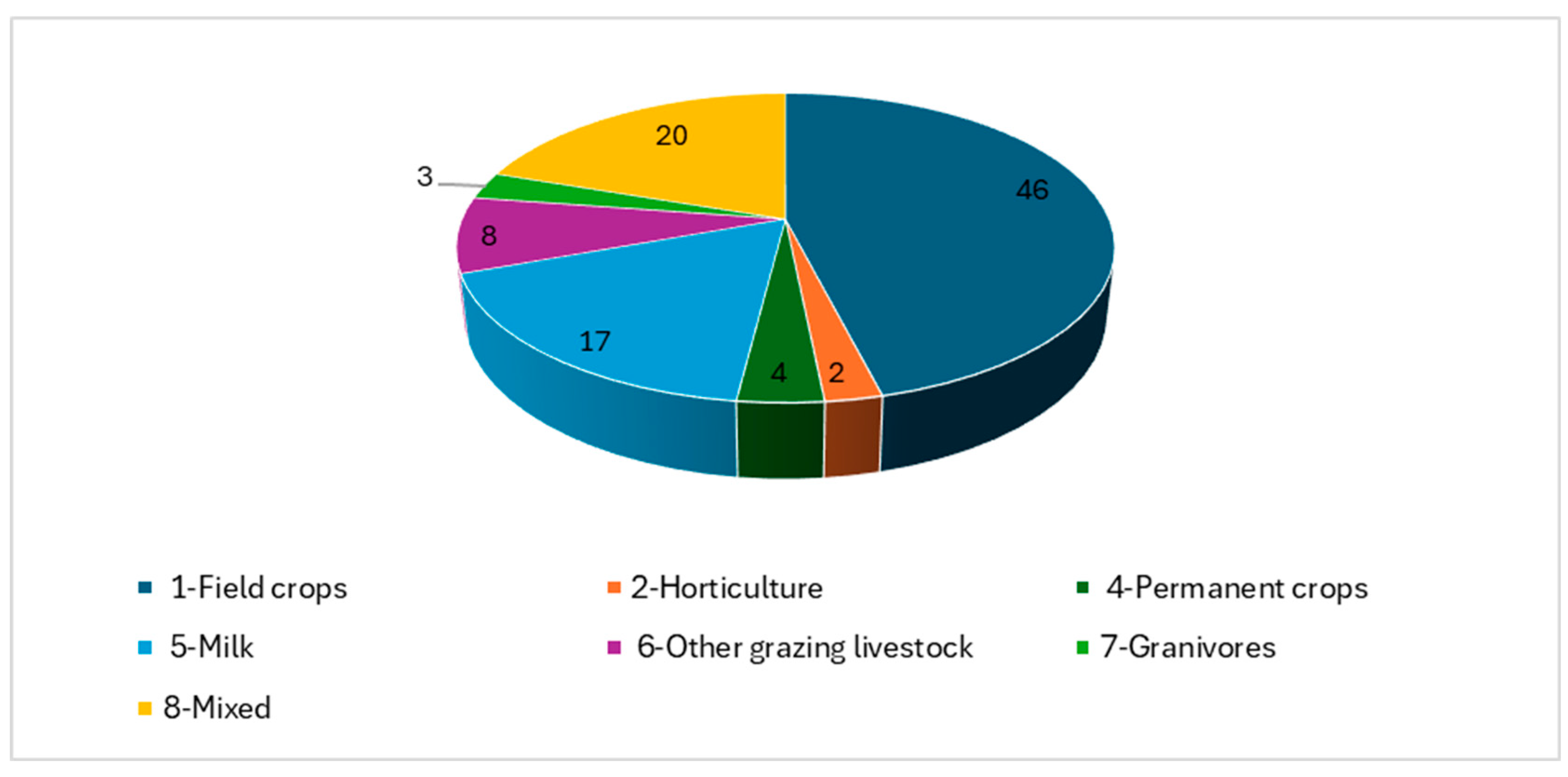
The study utilised individual data from the 2023 FADN database. This is the latest data at the time of the research. The division of farms into types in accordance with the Community Typology of Agricultural Holdings was applied.

In this way, eight groups of farms (TF8) are distinguished, i.e.,

• Fieldcrops;
• Horticulture;
• Wine;
• Other permanent crops;
• Milk;
• Other grazing livestock;
• Granivores;
• Mixed.

The study omits the third type of farms, i.e., Wine Farms, which are not included in the study as part of the Polish FADN due to the relatively small scale of production of this type in Poland. Types 1–7 indicate that the farm is specialised in a specific profile of agricultural activity, while Type 8 indicates multidirectional farms, which are non-specialised with mixed plant and animal production. If a farm obtains at least 2/3 of the standard output value from a specific type of agricultural activity, it is classified as one of the 1–7 types; otherwise, if the farm diversifies sources of standard output value, it is considered a mixed one (type 8).

2.4. GHG Calculation Stages—IPCC Basis vs. Assumptions and Estimations Adopted to FADN

Based on the IPCC methodology and the scope of the FADN data, emissions from the Agricultural sector were estimated for the study. Emissions from the energy sector were partially taken into account, while emissions from Sector 5, i.e., land change, were omitted. The lack of estimates results from the inability to calculate them based on the available data.

As a result, emissions were divided into the following sources, which were determined (calculated or estimated):

• Emissions of livestock origin.
• Direct emissions from soils.
• Indirect emissions from soils.
• Field burning of agricultural residues.
• Emissions from fuel combustion.
• Emissions from electricity consumption.

Ad. (1) Emissions of livestock origin

As part of the emissions from livestock origin, three variables were considered: CH₄ emissions from the enteric fermentation process and the emissions of two gases (CH₄ and N₂O) from manure management processes. The method used to calculate emissions is shown in

Table 3. Emissions of livestock origin.

Emission Source	GHG	Calculation Method
Enteric Fermentation	kg CH4	=The size of the population of the livestock species × indicator
Manure Management	kg CH4	=The size of the population of the livestock species × indicator
	kg N2O	=The size of the population of the livestock species × indicator

Source: own study.

. The calculations used indicators for 2022, i.e., the latest ones published by the KOBiZE (2024). Their list is presented in

Table 4. Livestock emission indicators for 2022.

Emission Source	Enteric Fermentation	Manure Management
Compound	CH4	CH4	N2O
	(kg CH4/head/yr)	(kg CH4/head/yr)	(kg N2O/head/yr)
Dairy Cattle	127.00	8.25	0.88
Non-dairy young cattle (younger than 1 year)	41.47	1.62	0.34
Non-dairy young cattle 1–2 years	59.14	1.62	0.34
Non-dairy heifers (older than 2 years)	46.01	1.62	0.34
Bulls (older than 2 years)	89.49	1.62	0.34
Sheep	8.00	0.19	0.04
Swine	1.50	2.29	0.09
Goats	5.00	0.13	0.03
Horses	18.00	1.56	0.33
Poultry	-	0.03	0.00

Source: own study based on KOBiZE.

. It is worth noting that these indicators are the result of complex calculations carried out by KOBiZE and are subject to change in the future. For this reason, appropriate indicators should be used for each year included in the research. In the present case, due to the lack of publication of indicators for 2023, it was decided to use the most recent ones, e.g., for 2022.

Ad. (2) Direct emissions from soils

Estimating direct emissions from soils is the most complex area of analysis. As part of the analysis, these emissions were divided into two groups, i.e.,

(a)

related to the use of mineral fertilisers and

(b)

into other sources.

This division is a result of the needs of this research, not the IPCC methodology. Such a division was aimed at emphasising the role of mineral fertilisation in the emission of the farm. In the first group, there are three processes: emissions from nitrogen mineral fertilisers, from urea, and from liming. The method of their calculation is presented in

Table 5. Method for calculating emissions from mineral fertilisers.

Emission Source	Emission	Calculation Method
Nitrogen mineral fertilisers	kg N2O	=[(the amount of mineral fertiliser used in the pure component N (kg) × emission factor)] × (44/28)
CO2 emissions from liming	kg CO2	=[(the amount of calcium fertilisers used on the farm, calculated in the pure CaO component (t) × emission factor)/1000] × (11/3)
CO2 emissions from urea	kg CO2	=[(the amount of calcium fertilisers used on the farm, calculated in the pure N component (t) × urea index)/1000] × emission factor) × (11/3)

Source: own study based on KOBiZE [60].

.

The emission factor means that 1 kg of nitrogen mineral fertiliser emits 0.01 kg of N₂O-N. The fraction 44/28 is used for the conversion of kg N₂O-N/kg N to kg N₂O.

Based on FADN data, it is not possible to accurately calculate the amount of urea used. For this reason, an indirect method of calculating these emissions was adopted, based on the conversion of the amount of nitrogen fertilisers used by an appropriate factor, which in 2023 amounted to 24.2%. This figure is based on market data, which indicates the share of urea in sales of mineral nitrogen fertilisers. The Emission Index for Urea means that 1 t of urea emits 0.2 t of CO₂-C.

In the case of liming, the Polish FADN database also does not contain direct quantitative data on lime fertilisers. For this reason, it is necessary to estimate this value indirectly by adopting an appropriate coefficient based on market data for the agricultural sector, which indicates the average price of CaO and the average share of CaO in lime fertilisers. However, these data change annually, requiring adequate calculations. The emission factor is 0.12, which means that 0.12 t of CO₂-C is emitted from 1 t of CaO.

The fraction 11/3 refers to the conversion of kg CO₂-C to kg CO₂.

In the second group of other direct emission processes from soils, three processes were also taken into account, i.e.,

• Emissions from organic N fertilisers use animal manure;
• Emissions from urine and dung deposited by grazing animals;
• Emissions from crop residues (Table 6).

Table 6. Method for calculating emissions from soils of natural origin (kg N₂O).

Process	Calculation Method
Organic N fertilisers use animal manure	=[(number of animals of a given species and by age × total amount of nitrogen in animal excreta (Nex) × fraction of total annual nitrogen excretion for each livestock category managed in manure management system (MS)) × (1 − the amount of manure nitrogen for the animal category of the species and age that is lost in the manure management system)] × (44/28)
Urine and dung deposited by grazing animals	=[number of animals of a given species and by age × total amount of nitrogen in animal excreta (Nex) × fraction of total annual nitrogen excretion for each livestock category managed in manure management system (MS)] × (44/28)
Crop residues	={harvested annual dry matter yield for crop × [ratio of above-ground residues dry matter to harvested yield for crop (RAG(T)) × N content of above-ground residues for crop (NAG(T)) × (1 − fraction of crop residues burned (FracBurn(T)) − fraction of above-ground residues of crop T removed annually for purposes such as feed, bedding and construction (FracRemove(T)))] + ratio of below-ground residues to harvested yield for crop (RBG(T)) × content of below-ground residues for crop (NBG(T))} × 0.01 × (44/28)

Source: own study based on KOBiZE [60] and IPCC [58].

Table 6. Method for calculating emissions from soils of natural origin (kg N₂O).

Process	Calculation Method
Organic N fertilisers use animal manure	=[(number of animals of a given species and by age × total amount of nitrogen in animal excreta (Nex) × fraction of total annual nitrogen excretion for each livestock category managed in manure management system (MS)) × (1 − the amount of manure nitrogen for the animal category of the species and age that is lost in the manure management system)] × (44/28)
Urine and dung deposited by grazing animals	=[number of animals of a given species and by age × total amount of nitrogen in animal excreta (Nex) × fraction of total annual nitrogen excretion for each livestock category managed in manure management system (MS)] × (44/28)
Crop residues	={harvested annual dry matter yield for crop × [ratio of above-ground residues dry matter to harvested yield for crop (RAG(T)) × N content of above-ground residues for crop (NAG(T)) × (1 − fraction of crop residues burned (FracBurn(T)) − fraction of above-ground residues of crop T removed annually for purposes such as feed, bedding and construction (FracRemove(T)))] + ratio of below-ground residues to harvested yield for crop (RBG(T)) × content of below-ground residues for crop (NBG(T))} × 0.01 × (44/28)

Source: own study based on KOBiZE [60] and IPCC [58].

In this group, due to the lack of data, emissions from fertilisers of urban origin and emissions from histosols were omitted. The calculation of emissions belonging to this group should be classified as one of the most complex processes.

N₂O emissions from the use of organic nitrogen fertilisers require a number of calculations and assumptions. The starting point is to calculate the amount of fertilisers that have been used on the farm in the pure component. Based on FADN data, it is possible to calculate the main source of organic fertilisers, namely, the amount of fertilisers from the farm. Fertilisers from sewage systems and natural fertilisers traded on the market from/to the farm were omitted due to the lack of relevant data. Given the negligible market for trade in natural fertilisers, these figures do not significantly affect the overall estimate.

Estimating the amount of manure available on a farm involves a series of complex calculations, as outlined in Table 6. For this study, calculations were performed under conditions prevailing in Poland. Based on this, it is necessary to calculate the amount of nitrogen available for use in fertilisation. This requires calculating and subtracting from the total available organic nitrogen the part that remained in the form of faeces on pasture and was oxidised. Calculations should be made for the same species that were taken into account when calculating emissions of animal origin. Due to the lack of adequate information on the use of mulching, this element was not included in the FADN calculations. Emissions from this source should be added to the result obtained for each source.

The Nex(T) (

Table 7. Nex(T) indicators for selected species of livestock in 2022 (kg N/animal/year).

Species	Other Cattle (Weighted Mean)	Dairy Cattle	Non-Dairy Young Cattle (Younger than 1 Year)	Non-Dairy Young Cattle 1–2 Years	Non-Dairy Heifers (Older than 2 Years)	Bulls (Older than 2 Years)
Coefficient	51.26	122.37	44.56	55.69	51.36	85.48
Species	Sheep	Horses	Swine (weighted mean)	Piglets (<20 kg)	Piglets (20–50 kg)	Fattening pigs (>50 kg)
Coefficient	9.5	55	10.95	2.6	9	15
Species	Butcher hogs	Sows	Goats	Hens	Broilers	Ducks
Coefficient	18	20	8	0.725	0.435	1.381
Species	Turkeys	Geese	Rabbits	Minks and polecats	Foxes, raccoons
Coefficient	1.554	1.64	8.1	4.59	12.09

Source: KOBiZE [60].

) and MS(T, S) indices (cf.

Table 8. MS indicators for selected species of livestock in 2022 (in %).

Type MS	Liquid System	Solid Storage and Dry Lot	Pasture, Range, and Paddock
Dairy cattle	12.60	79.30	8.20
Non-dairy cattle	6.40	77.80	15.80
Swine	59.70	40.30	0.00

Source: own study based on KOBiZE data.

) vary by year and are published by KOBiZE.

The result of the estimation should be multiplied by the appropriate emission index, which is 0.001 for poultry and 0.005 for other animals considered in the FADN system.

To calculate emissions from urine and dung deposited by grazing animals, the number of animals of a given species and age is multiplied by the Nex indicator (Table 7) and by the MS indicator presented in Table 8. The sum of emissions for individual animals is the amount of emissions for the farm from manure left on pastures, ranges, and paddocks.

Emissions from crop residues left in the fields are calculated separately for each crop. The counting method is presented in Table 6. The indicators necessary to calculate emissions are presented in

Table 9. Indicators for calculating the crop residues.

Indicator	NAG(T) (kg N/kg d.m.)	FracBurn(T)	FracRemove(T) (kg N/kg Crop-N)	NBG(T) (kg d.m./kg d.m.)	RBG-BIO (kg N/kg d.m.)	AGDM(T) (Mg/ha)
						Slope	Intercept
Wheat	0.006	0.005	0.7	0.009	0.24	1.51	0.52
Barley	0.007	0.005	0.7	0.014	0.22	0.98	0.59
Maize for grain	0.006	0.002	0.1	0.007	0.22	1.03	0.61
Oats	0.007	0.004	0.7	0.008	0.25	0.91	0.89
Rye	0.005	0.005	0.7	0.011	0.22	1.09	0.88
Triticale	0.006	0.005	0.7	0.009	0.22	1.09	0.88
Cereals mixed	0.006	0.004	0.7	0.009	0.22	1.09	0.88
Millet and buckwheat	0.006	0.002	0.7	0.009	0.22	1.43	0.14
Pulses	0.006	0.001	0.1	0.008	0.19	1.13	0.85
Potatoes	0.019	0.1	0.01	0.014	0.2	0.1	1.06
Rape and agrimony	0.006	0.03	0.2	0.009	0.22	1.09	0.88

Source: Own study based on KOBiZE [60] and IPCC [58].

.

Additionally, it is necessary to calculate the R_AG(T) (Formula (1)) and R_BG(T) (Formula (2)). The method for calculating these indicators is presented in the IPCC guide [58].

R_AG(T) = [(AG_DM(T) × 1000 + Crop(T))/Crop(T)],

(1)

R_BG(T) = (R_BG-BIO × AG_DM(T) × 1000 + Crop(T))/Crop(T),

(2)

To calculate them, it is necessary to calculate the Above-ground residue dry matter (AG_DM(T)) index (Formula (3)).

AG_DM(T) = (Crop_(T)/1000) × slope_(T) + intercept_(T),

(3)

Indicators necessary for the calculation of R_BG(T) and AG_DM(T) are presented in Table 9.

Ad. (3) Indirect emissions from soils

Indirect emissions from soils are calculated based on two processes: atmospheric nitrogen volatilisation and nitrogen leaching and runoff. In both cases, the issue concerns N₂O.

To calculate the amount of volatilised nitrogen, it is necessary to multiply the amount of mineral nitrogen in the pure component by 0.1. To this result, the sum of nitrogen from organic fertilisation, with the nitrogen left in the field, multiplied by 0.2, should be added. The number calculated in this way should be multiplied by the emission factor of 0.01. The result obtained should be multiplied by 44/28 and then by the GWP index.

In the case of leaching and runoff, the sum of all available nitrogen, i.e., nitrogen used for mineral and organic fertilisation and left by animals on pastures and in crop residues, should be multiplied by 0.3 and then by 0.0075. The value obtained in this way should be reduced to the appropriate unit, i.e., CO₂ equivalent, by multiplying successively by 44/28 and by the GWP index.

The result of the sum of the above calculations is the amount of indirect emission.

Ad. (4) Emissions from the field burning of agricultural residues

Field burning of agricultural residues is a marginal practice, as it is prohibited by the GAEC 3 standard [61]. However, due to historical experience and exceptional situations, e.g., fires, it is still included in national reports. Using FADN data, emissions from this source can be calculated using an indirect method, similar to calculations made by KOBiZE for the entire agricultural sector. As a result, this emission is calculated separately for each cultivated plant. To do this, one can multiply the harvest volume in tonnes by the corresponding proportion of the crop left in the fields. The result obtained should be multiplied by the emission factors for CH₄ and N₂O. The relevant indicators are presented in

Table 10. Indicators needed to calculate emissions from crop residue incineration.

Indicator	Share of the Crop Left to Burn	Emission Indicator N2O/t	Emission Indicator CH4/t
Wheat	0.005	0.07	3.24
Barley	0.005	0.08	3.04
Maize	0.002	0.10	3.14
Oats	0.004	0.08	3.13
Rye	0.005	0.06	3.20
Triticale	0.005	0.07	3.24
Cereals mixed	0.004	0.08	3.15
Millet	0.002	0.10	3.00
Pulses	0.001	0.22	3.00
Potatoes	0.1	0.22	2.82
Rape and agrimony	0.03	0.07	3.00
Vegetables	0.01	0.28	3.00
Fruits	0.1	0.16	3.00

Source: own study based on KOBiZE [60].

.

The sum of the results obtained for all crops is the number of emissions from the combustion of crop residues.

Ad. (5 and 6) Emissions from fuels and electricity consumption

Emissions from energy use were also included in the study. Two sources of energy, i.e., fuel and electricity, were taken into account. In the Polish FADN, data on energy consumption is collected only in the form of the costs of its consumption. This applies to electricity and fuel. Therefore, these data were the starting point for determining the estimated amount of consumption in physical units.

In the case of fuels, it was assumed that the total energy consumption is for diesel oil. As a result, fuel costs were divided by the annual average diesel price in 2023 to calculate the amount of consumption. It amounted to 6.7 PLN/L (calculated based on data from official statistics). Emissions are calculated by multiplying the amount of fuel consumed by the corresponding emission factor for that fuel, which in transport is 2.64 kg CO₂/L.

In the case of electricity, the cost of this energy from the FADN database was divided by the average price of electricity, which in 2023 was 0.7840 PLN/kWh [62]. The result obtained was multiplied by 3.6 to convert units from kWh/kg to MJ/kg emission factor for the specified year. This indicator is published every year in the relevant regulation of the Minister of Climate and Environment. For 2023, this indicator is 182.1 gCO₂ eq/MJ [63]. The result obtained should be divided by 1000 to obtain the emission in kilograms.

2.5. Calculating GHG Emissions per Farm

The results obtained regarding the emission of various greenhouse gases (carbon dioxide—CO₂, methane—CH₄, and nitrous oxide—N₂O) have been reduced to a common denominator, which is carbon dioxide equivalent. The conversion was made using Global Warming Potential (GWP) indicators for a 100-year period, as per the latest IPCC Sixth Report [20], i.e., for CO₂—1, for CH₄—27.9, and for N₂O—273.

The sum of the above partial emissions is the total GHG emissions per farm expressed in eq. CO₂ kg.

3. Results

3.1. Farm Number

The presented research method was used to estimate the amount of GHG emissions at the farm level. The calculations were carried out for all farms covered by FADN in 2023, i.e., 11,029 farms. For the studied population, the basic characteristics of production potential, economic potential, and organisation of production were determined, and then the sources and volume of emissions, which were particularly important, were assessed. The results were illustrated for the entire community as well as for individual types of agricultural farms—farming types.

3.2. Farms’ Production and Economic Potential; Farms’ Organisation

In the surveyed population of farms using FADN agricultural accounting, most farms focused on field crop production (type 1)—nearly half of the farms (5078 farms, Figure 2). Every fifth farm carried out non-specialised production, i.e., combined crop and livestock production (type 8), without the dominance of any of the directions of agricultural production (2184 farms). The next largest were farms specialising in milk production (type 5, 1923 farms). These three types account for over 80% of FADN farms, which are responsible for commodity production. Other specialised units, which together represented 17% of the analysed population, were farms focused on rearing other ruminant animals—mainly cattle (type 6), granivores (type 7), or permanent crops (type 4) and horticultural crops (type 2). Despite these differences, due to the large number of each farm type included in the FADN, the analysis of GHG was carried out in the order of farming types, highlighting important elements of the calculation that correspond to the specificity of their agricultural production.

As indicated in the part of the article devoted to the method of GHG estimation, the scale of emissions depends on the production potential of farms and their organisation. The productive potential of farms is evidenced by the size (resources and inputs) of their factors of production, namely the area of land, labour, and the value of capital. The specificity of FADN farms in Poland is illustrated in

Table 11. An average FADN farm’s characteristics of production and economic potential, including farming types ¹.

Specificity of Average Farm	In Total	Type 1	Type 2	Type 4	Type 5	Type 6	Type 7	Type 8
Total Utilised Agricultural Area (ha)	30.8	35.8	6.5	10.1	30.6	24.0	32.0	28.8
Total Labour Input (Annual Work Units) 2	1.6	1.4	2.6	1.9	1.9	1.5	2.0	1.6
Total Assets (Thousand Euro)	367.4	369.8	162.6	194.9	441.9	284.8	564.0	356.7
Total Livestock 3 (Livestock Units)	19.8	1.6	0.5	0.0	45.9	24.6	147.5	24.8
Livestock density (Livestock Units/ha)	0.6	0.0	0.1	0.0	1.5	1.0	4.6	0.9
Cattle (Livestock Units, LU)	12.9	0.9	0.4	0.0	45.8	23.2	0.9	13.0
Dairy cows (Livestock Units)	5.7	0.1	0.0	0.0	28.5	1.7	0.0	2.7
Pigs (Livestock Units)	6.2	0.5	0.1	0.0	0.1	0.1	129.8	11.1
Sheep and goats (Livestock Units)	0.1	0.0	0.0	0.0	0.0	0.5	0.0	0.2
Poultry (Livestock Units)	0.6	0.0	0.0	0.0	0.0	0.0	16.8	0.3
Standard Output (Thousand Euro) 4	50.2	39.2	85.5	25.4	71.7	32.3	172.0	47.0
Gross margin (Thousand Euro) 5	35.3	25.3	49.9	28.4	66.6	17.6	103.8	27.8

¹ Farming types: 1—Field crop, 2—Horticulture, 4—Permanent crops, 5—Milk, 6—Other grazing livestock, 7—Granivores, 8—Mixed. ² Labour Input expressed in Annual Work Units that are equal to 2120 working hours per year. ³ Number of equidae, cattle, sheep, goats, pigs, and poultry present on holding in annual average terms, converted into livestock units (LU). Not included are beehives, rabbits, and other animals. Animals which do not belong to the holder but are held under a production contract are taken into account for their annual presence. Indicators of LU: Equines = 0.8; Dairy cows = 1.0; Breeding sows = 0.5; Heifers for fattening = 0.8; Cull dairy cows = 1.0; Pigs for fattening = 0.3; Other cattle < 1 year = 0.4; Other cows = 0.8; Other pigs = 0.3; Male cattle 1–2 years = 0.7; Goats (breeding females) = 0.1; Table chickens = 0.007; Female cattle 1–2 years = 0.7; Other goats = 0.1; Laying hens = 0.014; Male cattle ≥ 2 years = 1.0; Ewes = 0.1; Other poultry = 0.03; Breeding heifers = 0.8; Other sheep = 0.1; Rabbits (breeding females) = 0.02; Calves for fattening = 0.4; Piglets = 0.027 [64]. ⁴ The Standard Output (SO) is an average five-year output value from a specified (crop or livestock) agricultural activity, obtained from 1 ha or 1 head of livestock per year, in the production conditions typical of a given region. To eliminate the impact of the production changes (e.g., caused by unfavourable weather conditions), or the impact of the products’ prices, average values for 5 years in the relevant period, based on the average annual data for a given region, were used in the calculations” [64]. ⁵ The exchange rate of 1 Euro = PLN 4.17347 [64]. Source: Own calculations based on FADN 2023 data.

.

The average analysed farm had an area of approximately 30 ha, about 1.6 AWU with labour inputs, and the value of its assets amounted to about EUR 370,000. About 20 LU animals were kept on such a farm. The livestock population was primarily composed of cattle, with pigs also present. Currently, sheep and goat breeding is a niche in agricultural production. Poultry production does not distinguish the average farm. An average FADN farm produces a standard production of 50,000 euros per year.

The profile of an average farm differs significantly when taking into account the specificity of production and the types of agricultural farms. Farms focused on specialised field crop production (type 1) are distinguished by relatively the largest acreage, low labour inputs, and assets similar to the average FADN farm. Livestock production in this case is niche—it is supplementary, but it is of production importance due to the natural fertilisers obtained. Other specialised farms dealing with crop production—i.e., horticulture (type 2) or permanent crops (type 4)—are much smaller, less than 10 ha, but they are distinguished by higher labour intensity and the lowest average value of assets. On the other hand, in the case of specialised farms involved in livestock production (milk production—type 5, rearing of other ruminant animals—type 6, pig breeding—type 7), the area and labour inputs are similar to the average FADN farm, but a high number of animals and livestock density distinguish them. In this respect, type 7—granivore farms are in the lead, which indicates a high scale of animal production. Considering the categories of livestock in specialised farms, it can be concluded that, apart from the main direction of livestock production, other groups of animals are not kept, which simultaneously confirms their professionalisation and focus on a specific type of agricultural activity.

In terms of economic potential, measured by the economic size determined based on the standard output value of the farm, the leaders are specialised granivore farms (type 7, almost 3.5 times larger than the average surveyed farm), followed by specialised horticulture (type 2, larger by 70%) and specialised farms focused on milk production (type 5, larger by over 40%) (Table 11). In the case of these units, the dominant part of farms generates standard production of at least EUR 25,000, i.e., these are farms with medium or high economic potential (Figure 3). It is worth noting that in the case of granivore farms (type 7), more than half are large or very large in economic terms and produce an average annual income of at least EUR 100,000. At the opposite end of the spectrum are specialist farms with permanent crops (type 4), field farms (type 1), and mixed-non-specialised farms (type 8), where about half of the farms are very small or small farms (less than 25,000 euros of standard production produced).

3.3. GHG Sources and Their Significance in the Context of Farming Types

In accordance with the adopted method for GHG estimation, several main groups of gas emission sources from farms have been distinguished (

Table 12. An average FADN farm’s GHG emission (t eq. CO₂ per farm), including farming types.

Specificity of GHG Sources	In Total	Type 1	Type 2	Type 4	Type 5	Type 6	Type 7	Type 8
Livestock emission	47.69	3.41	1.44	0.04	161.66	78.26	70.05	48.94
Agricultural soils, including:	22.63	24.04	3.18	3.44	29.78	14.68	30.00	20.97
-N fertilisers	16.78	22.11	2.74	3.00	14.54	6.64	15.92	14.72
-Urea	0.55	0.72	0.09	0.10	0.47	0.22	0.52	0.48
-Lime fertilisers	0.68	0.85	0.21	0.33	0.57	0.26	1.08	0.63
-Natural fertilisers	3.24	0.24	0.09	0.00	9.68	4.69	12.37	3.60
-Pastures	1.38	0.12	0.05	0.00	4.52	2.88	0.11	1.54
Burning residues in the field	0.30	0.41	0.17	1.39	0.05	0.04	0.17	0.20
Crop residues	7.00	11.25	0.75	0.39	1.69	1.34	5.83	6.19
Indirect emission	11.02	10.60	1.19	1.06	15.88	7.93	20.71	10.51
Fuel	7.39	7.53	3.12	3.16	9.77	5.13	8.83	6.91
Electricity	2.56	1.23	6.21	2.34	4.98	1.58	10.94	2.29
GHG in CO2 eq in t per farm	98.58	58.47	16.06	11.81	223.82	108.97	146.53	96.03

Source: Own calculations based on FADN 2023 data.

). The average FADN farm emitted almost 100 t GHG eq. CO₂ per year. Similar emissions occurred in the case of farms with mixed crop and animal production (type 8). Two extreme groups stood out, namely farms specialising in field crops (types 1, 2, 4), where, depending on the type, emissions from the farm averaged from 12 to 58 t GHG eq. CO_2, and, on the other hand, those specialising in animal production, emitting from 109 to 224 t GHG eq. CO₂. The highest results in this respect were characteristic of farms with milk production (type 5).

In an average FADN farm, nearly half of the total emissions came from animal emissions, while the other half consisted of emissions from agricultural soils and other sources, including the burning of crop residues, indirect emissions, and fuel and electricity use. The structure was similar in the mixed production farm (type 8) and the granivores (type 7). On the other hand, in specialised farms mainly keeping cattle (types 5 and 6), the main source of emissions was livestock production (72% of the total emissions of the farm in this type). In farms specialising in crop production (types 1, 2, and 4), livestock production was a negligible source of emissions (up to 9%), which is due to the small number of livestock kept on these farms.

Emissions from agricultural soils on farms specialising in field crops (type 1) account for 41% of total emissions, with crop residues, indirect emissions, and fuel being the remaining sources of emissions (19%, 18%, and 13%, respectively). In the case of horticultural crops (type 2), energy is the primary source of emissions, followed by soils and fuel (39%, 20%, and 19%, respectively). By contrast, agricultural soils and fuel are the main sources of emissions for farms specialising in permanent crops (29% and 27%, respectively).

It should be emphasised that in the case of emissions from agricultural soils, nitrogen fertilisers are the main source of emissions, while calcium fertilisers, natural fertilisers, and emissions from pastures account for a negligible part of emissions from this source.

Unit results of emissions from livestock and per hectare of agricultural land vary across different farming types, largely due to the type of livestock kept on the farms (Figure 4). The lowest livestock emissions are observed in granivore farms (type 7), where pigs and poultry are primarily kept (approximately 475 kg CO₂ per LU), in contrast to farms with cattle (3500 and 3290 kg CO₂ per LU, types 5 and 6).

While land-use emissions (from agricultural soils, residue burning, crop residues, indirect emissions, fuel, and energy) that are associated with farm areas are more than 2000 kg CO₂ per ha UAA in speciality types with horticultural crops, milk production, and granivores (types 2, 5, and 7), there is an average of 1600 kg CO₂ per ha UAA for the FADN farm. The least emission-intensive farms are specialised farms with permanent crops (type 4; 1170 kg CO2 per ha UAA).

Taking into account the entire emissions from the farm in relation to the unit area, the division into specialised ones with livestock production (4500–7300 kg CO₂ per ha UAA) and crop production (1200–2500 kg CO₂ per ha UAA) is emphasised. The average picture is similar to mixed farms (type 8), with 3200 and 3300 kg CO₂ per ha UAA.

4. Discussion

The research aimed to present the method of GHG calculation at the farm level, taking into account its application aspect. The available data resources from agricultural holdings in the FADN system were used. The authors aimed to present the various stages of GHG calculation in meticulous detail, taking into account the type of GHG and the data sources used. Attention was also paid to information gaps in the FADN database. At the same time, an approach to estimating some of the missing information was proposed to carry out the calculation of GHG at the farm level as fully as possible, using agricultural accounting data collected in each EU Member State.

The presented coefficients, types, and categories of variables should be helpful in the scientific considerations of other researchers. Since the article highlights the need for the practical application of this method, researchers from EU countries where agricultural accounting is conducted within a unified system of FADN can conduct analogous calculations for their own country and farming types. The use of the same method and the same data sources allows comparisons to be made for commodity farms, also taking into account their production profile and economic size.

However, it should be noted that GHG emissions measured in EU countries may differ due to the use of different methodologies. Usually, this involves moving to a higher level of detail, i.e., from Tier I to Tier III. Additionally, emission factors change over time, which may be due to the use of a more accurate method of calculation or the specific circumstances of a given year. For example, the average GHG emissions from electricity consumption vary depending on the energy mix involved. The more low-carbon sources there are, the lower this indicator will be.

At the same time, the article draws attention to information gaps, which is an important voice in the discussion on the extension of the FADN data scope. We would like to add that, as of 2025, the FADN system has been transformed into the FSDN—Farm Sustainability Data Network—due to the expansion of the scope of collected data to include those related to social and environmental issues, as well as partly economic ones. However, despite the changes introduced, many important data points are still not covered by this monitoring, which would allow for a more precise estimation of GHG from farms. GHG calculation was not a priority for decision-makers, defining an extended range of data for the FSDN system. It can be assumed that the burden on farmers in providing data was taken into account.

The aforementioned gaps necessitate further research to explore more accurate indirect methods of GHG estimation. This could lead not only to improved methodologies but also to more precise estimates of farm emissions, thereby providing a greater understanding of how to reduce these emissions.

Based on the IPCC method adapted to the FADN data, estimates were made for all farms keeping accounts in 2023. The population of FADN farms included in the study consisted of over 11 thousand units. The article outlines the production specificity of these farms, which determines the size and type of greenhouse gas emissions.

Empirical analysis indicated that in the case of FADN in Poland, farms specialising in field crops, further mixed farms with both crop and livestock production, and those specialising in milk production dominate. These figures indicate that livestock production has a significant impact on the scale of emissions on the one hand, and crop production on the other. Thus, in both directions of production, diverse reduction practices are crucial to decrease the total sum of emissions from the farm and, subsequently, from the entire agricultural sector.

The types of farms differ significantly from each other in terms of production profile and production organisation, which determines their final impact on the amount of emissions. Taking into account the characteristics of FADN farms, the largest scale of emissions is considered for an average specialist farm with milk production, followed by a specialist farm with granivorous animals, then a specialist farm with other cattle, and a mixed farm with both crop and livestock production. These types of production emit more GHG than the average farm. In the case of type 5, which specialises in milk production, the emission is more than twice the average. Significantly lower emissions come from farms specialised in field crops, while the least emission-intensive, taking into account a given research method, are horticultural and permanent farms.

The relationship is slightly different if the emissions are counted per livestock unit. In this case, farms with granivorous livestock are most favourably located. Thus, the presented considerations indicate the need to use various indicators to assess the level of generated GHG emissions, highlighting their advantages and disadvantages. Assessing GHG emissions through the angle of a single indicator may not provide a complete picture.

Considering the types of emission sources and their impact on the total farm result, the impact varies between different farming types. For farms such as those specialised in milk production and those specialised in other cattle maintenance, more than 70% of a farm’s GHG emissions come from livestock emissions. For crop-specialised farms, 40% of emissions come from soils, while energy is the dominant source of GHG, accounting for almost 40% of total GHG emissions from horticultural farms. Thus, depending on the agricultural type, a different source of GHG emissions determines the total result. These data confirm the need for a comprehensive approach to reduction practices on farms, taking into account the different specificities of production.

The results of the study are difficult to compare with other similar estimates carried out in Poland on the basis of FADN data. In some cases [57], the authors do not provide emission estimates, but only the shares of individual groups of emission sources in the types of farms. In other cases [56], there are differences in the research method used, which can significantly affect the results obtained. However, even in the case of differences in absolute values, it is noted that the shares of emissions from different sources are similar.

The results obtained appear to be useful for implementing climate policy. Large differences in emissions between the types of farms identified in the FADN are a strong reason to consider targeting public aid. It seems that some of the support instruments under the Common Agricultural Policy (CAP) could be more specialised. This is visible when analysing emission sources in individual types. Such action would have to be supplemented by additional analyses showing the reduction possibilities for individual types of farms and economic analyses that provide a broader perspective, e.g., in the context of the profitability of individual types of farms.

5. Conclusions

• The results demonstrate that the presented method for calculating GHG emissions based on FADN data is suitable for achieving the goal of determining emissions at the farm level. The IPCC-based emission calculation method used requires that some FADN variables be adapted to the relevant units. For example, it requires calculating the amount of consumption of specific resources based on their average value.
• The application of the presented method requires adjusting the sub-indicators to the year in which the emission is calculated. Additionally, this method is tailored to the data and emission factors prevalent in Poland, but it can be adapted to FADN data from other countries. It is only necessary to use the indicators present in a given country.
• The results reveal significant differences in emissions among farm types. This applies to total emissions and emissions from various sources. This can be a significant indicator for farms in terms of climate policy priorities implemented at the farm level.
• On average, GHG emissions from energy used on a farm account for approximately 10% of total emissions, but this share varies depending on the type of farm. In the case of type 4, the share of energy emissions is over 46% of the GHG emissions from the farm. In absolute numbers, this is not much, but it shows that reducing emissions from the energy sector on farms can also have significant effects.
• The results obtained can also be an important clue for policymakers. They suggest that, to achieve better effects of climate policy with limited financial resources, it would be justified to direct political actions to select groups of farms, thereby targeting aid more effectively. However, this requires further in-depth research.

References

1. Johansen, B.E. Global Warming and the Climate Crisis: Science, Spirit, and Solutions; Springer: Dordrecht, The Netherlands, 2023. [Google Scholar] [CrossRef]
2. Intergovernmental Panel on Climate Change (IPCC). Climate Change 2021—The Physical Science Basis; Cambridge University Press: Cambridge, UK, 2023. [Google Scholar] [CrossRef]
3. Global Climate Highlights 2024|Copernicus. Available online: https://climate.copernicus.eu/global-climate-highlights-2024 (accessed on 3 July 2025).
4. EDGAR—The Emissions Database for Global Atmospheric Research. Available online: https://edgar.jrc.ec.europa.eu/country_profile (accessed on 2 July 2025).
5. Warren, R.; Arnell, N.; Nicholls, R.; Levy, P.; Price, J. Understanding the Regional Impacts of Climate Change; Tyndall Centre for Climate Change Research Working Paper; Tyndall Centre for Climate Change Research: Norwich, UK, 2006; Volume 90, p. 133. [Google Scholar]
6. Intergovernmental Panel on Climate Change (IPCC). Linking Global to Regional Climate Change. In Climate Change 2021—The Physical Science Basis: Working Group I Contribution to the Sixth Assessment Report of the Intergovernmental Panel on Climate Change; Cambridge University Press: Cambridge, UK, 2023; pp. 1363–1512. [Google Scholar]
7. Filonchyk, M.; Peterson, M.P.; Zhang, L.; Hurynovich, V.; He, Y. Greenhouse Gases Emissions and Global Climate Change: Examining the Influence of CO2, CH4, and N2O. Sci. Total Environ. 2024, 935, 173359. [Google Scholar] [CrossRef] [PubMed]
8. Raupach, M.R.; Marland, G.; Ciais, P.; Le Quéré, C.; Canadell, J.G.; Klepper, G.; Field, C.B. Global and Regional Drivers of Accelerating CO2 Emissions. Proc. Natl. Acad. Sci. USA 2007, 104, 10288–10293. [Google Scholar] [CrossRef] [PubMed]
9. Hui, D.; Deng, Q.; Tian, H.; Luo, Y. Global Climate Change and Greenhouse Gases Emissions in Terrestrial Ecosystems. In Handbook of Climate Change Mitigation and Adaptation, 3rd ed.; Springer International Publishing: Cham, Switzerland, 2022; Volume 1, pp. 23–76. [Google Scholar] [CrossRef]
10. Al-Ghussain, L. Global Warming: Review on Driving Forces and Mitigation. Environ. Prog. Sustain. Energy 2019, 38, 13–21. [Google Scholar] [CrossRef]
11. von Storch, H.; Flöser, G. (Eds.) Anthropogenic Climate Change; Springer: Berlin/Heidelberg, Germany, 1999. [Google Scholar]
12. Von Storch, H.; Stehr, N. Anthropogenic Climate Change: A Reason for Concern Since the 18th Century and Earlier. Geogr. Ann. Ser. A Phys. Geogr. 2006, 88, 107–113. [Google Scholar] [CrossRef]
13. Agnihotri, R.; Dutta, K. Anthropogenic Climate Change: Observed Facts, Projected Vulnerabilities and Knowledge Gaps. In Earth System Processes and Disaster Management; Sinha, R., Ravindra, R., Eds.; Springer: Berlin/Heidelberg, Germany, 2013; pp. 123–137. [Google Scholar] [CrossRef]
14. Babinszky, L.; Halas, V.; Verstegen, M.V.A. Impacts of Climate Change on Animal Production and Quality of Animal Food Products. In Climate Change Socioeconomic Effects; Kheradmand, H., Blanco, J., Eds.; IntechOpen: London, UK, 2011. [Google Scholar]
15. Heshmati, H. Impact of Climate Change on Life. In Environmental Issues and Sustainable Development; Sarvajayakesavalu, S., Charoensudjai, P., Eds.; IntechOpen: London, UK, 2020. [Google Scholar] [CrossRef]
16. Holt, R.D. The Microevolutionary Consequences of Climate Change. Trends Ecol. Evol. 1990, 5, 311–315. [Google Scholar] [CrossRef]
17. Olesen, J.E.; Trnka, M.; Kersebaum, K.C.; Skjelvåg, A.O.; Seguin, B.; Peltonen-Sainio, P.; Rossi, F.; Kozyra, J.; Micale, F. Impacts and Adaptation of European Crop Production Systems to Climate Change. Eur. J. Agron. 2011, 34, 96–112. [Google Scholar] [CrossRef]
18. Visser, M.E. Keeping up with a Warming World; Assessing the Rate of Adaptation to Climate Change. Proc. R. Soc. B Biol. Sci. 2008, 275, 649–659. [Google Scholar] [CrossRef]
19. WMO. WMO Global Annual to Decadal Climate Update 2025; WMO: Geneva, Switzerland, 2025. [Google Scholar]
20. Kikstra, J.S.; Nicholls, Z.R.J.; Smith, C.J.; Lewis, J.; Lamboll, R.D.; Byers, E.; Sandstad, M.; Meinshausen, M.; Gidden, M.J.; Rogelj, J.; et al. The IPCC Sixth Assessment Report WGIII Climate Assessment of Mitigation: From Emissions to Global Temperatures. Geosci. Model Dev. 2022, 15, 9075–9109. [Google Scholar] [CrossRef]
21. Randers, J. 2052: A Global Forecast for the Next Forty Years; Chelsa Green Publishing: White River Junction, VT, USA, 2012. [Google Scholar]
22. Rogelj, J.; Popp, A.; Calvin, K.V.; Luderer, G.; Emmerling, J.; Gernaat, D.; Fujimori, S.; Strefler, J.; Hasegawa, T.; Marangoni, G.; et al. Scenarios towards Limiting Global Mean Temperature Increase below 1.5 °C. Nat. Clim. Chang. 2018, 8, 325–332. [Google Scholar] [CrossRef]
23. Yalew, S.G.; van Vliet, M.T.H.; Gernaat, D.E.H.J.; Ludwig, F.; Miara, A.; Park, C.; Byers, E.; De Cian, E.; Piontek, F.; Iyer, G.; et al. Impacts of Climate Change on Energy Systems in Global and Regional. Nat. Energy 2020, 5, 794–802. [Google Scholar] [CrossRef]
24. Stern, N. The Economics of Climate Change. Am. Econ. Rev. 2008, 98, 1–37. [Google Scholar] [CrossRef]
25. Strapasson, A.; Woods, J.; Pérez-Cirera, V.; Elizondo, A.; Cruz-Cano, D.; Pestiaux, J.; Cornet, M.; Chaturvedi, R. Modelling Carbon Mitigation Pathways by 2050: Insights from the Global Calculator. Energy Strategy Rev. 2020, 29, 100494. [Google Scholar] [CrossRef]
26. Steel, D.; DesRoches, C.T.; Mintz-Woo, K. Climate Change and the Threat to Civilization. Proc. Natl. Acad. Sci. USA 2022, 119, e2210525119. [Google Scholar] [CrossRef] [PubMed]
27. UN. Transforming Our World: The 2030 Agenda for Sustainable Development; UN: New York, NY, USA, 2015. [Google Scholar]
28. European Commission. Communication from the Commission to the European Parliament, the European Council, the Council, the European Economic and Social Committee and the Committee of the Regions, the European Green Deal; European Commission: Brussels, Belgium, 2019. [Google Scholar]
29. European Commission. Communication from the Commission to the European Parliament, the Council, the European Economic and Social Committee and the Committee of the Regions a Farm to Fork Strategy for a Fair, Healthy and Environmentally-Friendly Food System; No. COM(2020) 381 Final; European Commission: Brussels, Belgium, 2020. [Google Scholar]
30. European Commission. Communication from the Commission to the European Parliament, the Council, the European Economic and Social Committee and the Committee of the Regions EU Biodiversity Strategy for 2030 Bringing Nature Back into Our Lives; COM/2020/380 Final; European Commission: Brussels, Belgium, 2020. [Google Scholar]
31. Lamb, W.F.; Wiedmann, T.; Pongratz, J.; Andrew, R.; Crippa, M.; Olivier, J.G.J.; Wiedenhofer, D.; Mattioli, G.; Khourdajie, A.A.; House, J.; et al. A Review of Trends and Drivers of Greenhouse Gas Emissions by Sector from 1990 to 2018. Environ. Res. Lett. 2021, 16, 073005. [Google Scholar] [CrossRef]
32. Malik, A.; Lan, J.; Lenzen, M. Trends in Global Greenhouse Gas Emissions from 1990 to 2010. Environ. Sci. Technol. 2016, 50, 4722–4730. [Google Scholar] [CrossRef]
33. Clémençon, R. 30 Years of International Climate Negotiations: Are They Still Our Best Hope? J. Environ. Dev. 2023, 32, 114–146. [Google Scholar] [CrossRef]
34. Stoddard, I.; Anderson, K.; Capstick, S.; Carton, W.; Depledge, J.; Facer, K.; Gough, C.; Hache, F.; Hoolohan, C.; Hultman, M.; et al. Three Decades of Climate Mitigation: Why Haven’t We Bent the Global Emissions Curve? Annu. Rev. Environ. Resour. 2021, 46, 653–689. [Google Scholar] [CrossRef]
35. European Commission. Communication from the Commission to the European Parliament, the Council, the European Economic and Social Committee, the Committee of the Regions and European Investment Bank. A Clean Planet for All A European Strategic Long-Term Vision for a Prosper-Ous, Modern, Competitive and Climate Neutral Economy; European Commission: Brussels, Belgium, 2018. [Google Scholar]
36. Nsabiyeze, A.; Ma, R.; Li, J.; Luo, H.; Zhao, Q.; Tomka, J.; Zhang, M. Tackling Climate Change in Agriculture: A Global Evaluation of the Effectiveness of Carbon Emission Reduction Policies. J. Clean. Prod. 2024, 468, 142973. [Google Scholar] [CrossRef]
37. Schils, R.; Olesen, J.E.; Kersebaum, K.C.; Rijk, B.; Oberforster, M.; Kalyada, V.; Khitrykau, M.; Gobin, A.; Kirchev, H.; Manolova, V.; et al. Cereal Yield Gaps across Europe. Eur. J. Agron. 2018, 101, 109–120. [Google Scholar] [CrossRef]
38. Malhi, G.S.; Kaur, M.; Kaushik, P. Impact of Climate Change on Agriculture and Its Mitigation Strategies: A Review. Sustainability 2021, 13, 1318. [Google Scholar] [CrossRef]
39. Mbewu, A.D.; Elephant, D.E.; Motsi, H.; Nyambo, P. Climate Change Effects on Water Footprint of Crop Production: A Meta-Analysis. Environ. Chall. 2024, 17, 101033. [Google Scholar] [CrossRef]
40. Hatfield, J.L.; Prueger, J.H. Temperature Extremes: Effect on Plant Growth and Development. Weather. Clim. Extremes 2015, 10, 4–10. [Google Scholar] [CrossRef]
41. Nardone, A.; Ronchi, B.; Lacetera, N.; Ranieri, M.S.; Bernabucci, U. Effects of Climate Changes on Animal Production and Sustainability of Livestock Systems. Livest. Sci. 2010, 130, 57–69. [Google Scholar] [CrossRef]
42. Rojas-Downing, M.M.; Nejadhashemi, A.P.; Harrigan, T.; Woznicki, S.A. Climate Change and Livestock: Impacts, Adaptation, and Mitigation. Clim. Risk Manag. 2017, 16, 145–163. [Google Scholar] [CrossRef]
43. Kumar, P.; Tokas, J.; Kumar, N.; Lal, M.; Singal, H.; Correspondence, P.; Kumar. Climate Change Consequences and Its Impact on Agriculture and Food Security. Int. J. Chem. Stud. 2018, 6, 124–133. [Google Scholar]
44. Wu, H.; Etienne, F. Effect of Climate Change on Food Production (Animal Products). In The Impacts of Climate Change: A Comprehensive Study of Physical, Biophysical, Social, and Political Issues; Elsevier: Amsterdam, The Netherlands, 2021; pp. 233–253. [Google Scholar] [CrossRef]
45. Prandecki, K. Global and European Climate Policy. Zagadnienia Ekon. Rolnej Probl. Agric. Econ. 2022, 372, 45–63. [Google Scholar] [CrossRef]
46. Bhatti, U.A.; Bhatti, M.A.; Tang, H.; Syam, M.S.; Awwad, E.M.; Sharaf, M.; Ghadi, Y.Y. Global Production Patterns: Understanding the Relationship between Greenhouse Gas Emissions, Agriculture Greening and Climate Variability. Environ. Res. 2024, 245, 118049. [Google Scholar] [CrossRef]
47. Huang, S.; Ghazali, S.; Azadi, H.; Movahhed Moghaddam, S.; Viira, A.H.; Janečková, K.; Sklenička, P.; Lopez-Carr, D.; Köhl, M.; Kurban, A. Contribution of Agricultural Land Conversion to Global GHG Emissions: A Meta-Analysis. Sci. Total Environ. 2023, 876, 162269. [Google Scholar] [CrossRef]
48. Vineis, P.; Mangone, L.; Belesova, K.; Tonne, C.; Alfano, R.; Strapasson, A.; Millett, C.; Jennings, N.; Woods, J.; Mwabonje, O. Integration of Multiple Climate Change Mitigation Actions and Health Co-Benefits: A Framework Using the Global Calculator. Environ. Health Perspect. 2024, 132, 125001. [Google Scholar] [CrossRef]
49. Harmonisation of Carbon Accounting Tools for Agriculture. 2023. Available online: https://farmpep.net/resource/harmonisation-carbon-accounting-tools-agriculture-scf0129 (accessed on 17 October 2024).
50. Dabkienė, V.; Baležentis, T.; Štreimikienė, D. Calculation of the Carbon Footprint for Family Farms Using the Farm Accountancy Data Network: A Case from Lithuania. J. Clean. Prod. 2020, 262, 121509. [Google Scholar] [CrossRef]
51. Coderoni, S.; Bonati, G.; D’Angelo, L.; Longhitano, D.; Mambella, M.; Papaleo, A.; Vanino, S. Using FADN Data to Estimate Agricultural GHG Emissions at Farm Level. In Proceedings of the Pacioli 20—Complex Farms Sustain, Farm Level Data Collect, Rome, Italy, 30 September–3 October 2012; pp. 86–102. [Google Scholar]
52. Bazzani, G.M.; Vitali, G.; Cardillo, C.; Canavari, M. Using FADN Data to Estimate CO2 Abatement Costs from Italian Arable Crops. Sustainability 2021, 13, 5148. [Google Scholar] [CrossRef]
53. Coderoni, S.; Esposti, R. CAP Payments and Agricultural GHG Emissions in Italy. A Farm-Level Assessment. Sci. Total Environ. 2018, 627, 427–437. [Google Scholar] [CrossRef] [PubMed]
54. Sieczko, L.; Koloszko-Chomentowska, Z.; Sieczko, A. Variability of Greenhouse Gas Emissions in Relation to Economic and Ecological Indicators from Cattle Farms. Energies 2024, 17, 1831. [Google Scholar] [CrossRef]
55. Koloszko-Chomentowska, Z.; Sieczko, L.; Trochimczuk, R. Production Profile of Farms and Methane and Nitrous Oxide Emissions. Energies 2021, 14, 4904. [Google Scholar] [CrossRef]
56. Gołasa, P.; Wysokiński, M.; Bieńkowska-Gołasa, W.; Gradziuk, P.; Golonko, M.; Gradziuk, B.; Siedlecka, A.; Gromada, A. Sources of Greenhouse Gas Emissions in Agriculture, with Particular Emphasis on Emissions from Energy Used. Energies 2021, 14, 3784. [Google Scholar] [CrossRef]
57. Syp, A.; Osuch, D. Assessing Greenhouse Gas Emissions from Conventional Farms Based on the Farm Accountancy Data Network. Pol. J. Environ. Stud. 2018, 27, 1261–1268. [Google Scholar] [CrossRef]
58. IPCC. 2006 IPCC Guidelines for National Greenhouse Gas Inventories, Prepared by the National Greenhouse Gas Inventories Programme; Eggleston, S., Buendia, L., Miwa, K., Ngara, T., Tanabe, K., Eds.; IGES: Hayama, Japan, 2006. [Google Scholar]
59. What Does Tier 1, Tier 2 and Tier 3 Data Mean?: Snapshot. Available online: https://snapshotclimate.com.au/faq/what-does-tier-1-and-tier-2-data-mean/ (accessed on 20 May 2025).
60. KOBiZE. Poland’s National Inventory Report 2024; KOBiZE: Warsaw, Poland, 2024. [Google Scholar]
61. Conditionality—European Commission. Available online: https://agriculture.ec.europa.eu/common-agricultural-policy/income-support/conditionality_en (accessed on 26 May 2025).
62. Średnie ceny Sprzedaży Energii Elektrycznej na Rynku Konkurencyjnym oraz dla Gospodarstw Domowych w 2023 r. były wyższe niż w 2022 r.—Aktualności—Urząd Regulacji Energetyki 2024. Available online: https://www.ure.gov.pl/pl/urzad/informacje-ogolne/aktualnosci/11857,Srednie-ceny-sprzedazy-energii-elektrycznej-na-rynku-konkurencyjnym-oraz-dla-gos.html (accessed on 21 May 2025).
63. Rozporządzenie Ministra Klimatu i Środowiska z dnia 15 Grudnia 2022 r. w Sprawie Wskaźnika Emisji Gazów Cieplarnianych dla Energii Elektrycznej w 2023 r. Available online: https://isap.sejm.gov.pl/isap.nsf/DocDetails.xsp?id=WDU20220002671 (accessed on 21 May 2025).
64. Floriańczyk, Z.; Osuch, D.; Płonka, R. 2023 Standard Results of Polish FADN Agricultural Holdings; Institute of Agricultural and Food Economics-National Research Institute: Warszawa, Poland, 2025. [Google Scholar]
Figure 1. Scheme of activities undertaken as part of the study.
Sustainability 17 06452 g001
Figure 2. Farming types of FADN farms (in percentage). Specialised in crop production—types 1, 2, and 4; specialised in livestock production—types 5, 6, and 7; not-specialised—type 8. Source: Own calculations based on FADN 2023 data.
Sustainability 17 06452 g002
Figure 3. Farms’ economic size 1 according to farming types (in percentage); Source: Own calculations based on FADN 2023 data. 1 Categories of economic size groups in Poland based on Standard output value (Euro): 1—Very small [4000 Euro; 8000 Euro), 2—Small [8000 Euro; 25,000 Euro), 3—Medium-small [25,000 Euro; 50,000 Euro), 4—Medium-large [50,000 Euro; 100,000 Euro), 5—Large [100,000 Euro; 500,000 Euro), 6—Very large [500,000 Euro and more].
Sustainability 17 06452 g003
Figure 4. GHG emissions per unit, according to farming types (kg CO2 per unit). Source: Own calculations based on FADN 2023 data.
Sustainability 17 06452 g004