Operational Evaluation of Mixed Flow on Highways Considering Trucks and Autonomous Vehicles Based on an Improved Car-Following Decision Framework

Abstract

This study proposes a new method to improve the accuracy of car-following models in predicting the mobility of mixed traffic flow involving trucks and automated vehicles (AVs). A classification is developed to categorize car-following behaviors into eight distinct modes based on vehicle type (passenger car/truck) and autonomy level (human-driven vehicle [HDV]/AV) for parameter calibration and simulation. The car-following model parameters are calibrated based on the HighD dataset, and the models are selected through minimizing statistical error. A cellular-automaton-based simulation platform is implemented in MATLAB (R2023b), and a decision framework is developed for the simulation. Key findings demonstrate that mode-specific parameter calibration improves model accuracy, achieving an average error reduction of 80% compared to empirical methods. The simulation results reveal a positive correlation between the AV penetration rate and traffic flow stability, which consequently enhances capacity. Specifically, a full transition from 0% to 100% AV penetration increases traffic capacity by 50%. Conversely, elevated truck penetration rates degrade traffic flow stability, reducing the average speed by 75.37% under full truck penetration scenarios. Additionally, higher AV penetration helps stabilize traffic flow, leading to reduced speed fluctuations and lower emissions, while higher truck proportions contribute to higher emissions due to increased traffic instability.

1. Introduction

Highways serve as crucial corridors for passenger and freight transportation over medium and long distances. With the growing demand for highway transportation, the impacts of mixed passenger–freight traffic flow on mobility, safety, and environmental sustainability have become increasingly significant. Traffic congestion and flow instability not only reduce operational efficiency but also lead to higher fuel consumption and increased emissions, posing challenges to sustainable transportation development. Meanwhile, automated driving technology has developed rapidly, and recent reports predict that the penetration rate of L4-level automated vehicles (AVs) on urban roads will reach 24.8% by 2045 [1]. These trends indicate that future highway traffic flow will involve complex mixtures of different vehicle types (passenger cars/trucks) and autonomy levels (human-driven vehicle [HDV]/AV). Understanding and accurately modeling the interactions among these diverse vehicles is essential for optimizing traffic flow, improving road capacity, and reducing emissions, thereby contributing to the goals of sustainable and green transportation systems.

The theory of car following primarily uses dynamic methods to study single-lane traffic, where the rear vehicle follows the front vehicle under no-overtaking conditions. The different aspects of this car-following process can be represented through mathematical modeling. Car-following modeling has long been a key focus in traffic flow theory. As research has advanced, car-following models have become a central issue in the study of microscopic traffic flow. In general, car-following models are categorized into five types based on differences in driver response behavior during the car-following process. These types are Safety Distance Class, Optimal Speed Class, NaSch Class, Intelligent Driver Class, and Autonomous Driving Class.

Table 1. Comparative analysis of characteristics and differences among various car-following models.

Car-Following Model	Model Concept	Relevant Model	Advantages of the Model	Disadvantages of the Model
Safety Distance Model	Assume that the driver of the following vehicle expects to maintain a desired distance from the leading vehicle	Gipps model [2]	The model parameter calibration is relatively simple and can accurately simulate various traffic flow phenomena on the road	There is a discrepancy between the vehicle time headway and actual traffic conditions
Optimal Velocity Model	Assume that the vehicle aims to maintain an ideal safe velocity based on the difference in distance	FVD model [3], OV model [4], and GF model [5]	A relatively realistic representation of car-following behavior	When there is a significant velocity difference, it becomes difficult to ensure a safe time headway
NaSch Model	Simulate the dynamic behavior of vehicles on the road through simple rules and interactions between individuals	NaSch model [6], TT model [7], and VDR model [8]	The model is simple to understand, flexible to expand, and naturally captures phase transitions in traffic flow	The model imposes strict safety distance constraints but overlooks the impact of relative velocity
Intelligent Driving Model	It is assumed that the driver has a certain level of perception ability and aims to eliminate the difference from the desired velocity	IDM model [9]	The simulation results exhibit a small error compared to actual traffic data	The model has a large number of parameters
Autonomous Driving Model	Information sharing and cooperative control enhance the efficiency and safety of car following	CACC model [10]	The model has a simple structure, allowing for faster and more accurate responses based on the lead vehicle’s velocity and distance headway	Ignores communication delays and failures between vehicles

compares and outlines the characteristics and differences among these five car-following model types.

Modeling mixed traffic flow requires tailored approaches to account for the diverse interactions between different vehicle types and automation levels. Early research focused on the coexistence of passenger cars and trucks, driven by their distinct operating features. Trucks, which handle about 74% of total freight transport, have unique features—such as large size, slower acceleration/deceleration, and greater safety distances—that significantly affect highway performance. Initial car–truck mixed traffic models mainly focused on vehicle-specific parameters. For example, Jia [11] and Ebersbach et al. [12] used hybrid cellular automata to examine how vehicle length, speed, and truck proportions influence traffic flow. Meng et al. [13] expanded this framework to highway work zones by considering differences in vehicle size and movement patterns. Later studies, such as those by Moridpour [14] and Kong [15], found two-way behavioral interactions: cars change their following behavior near trucks, and trucks also adjust when following cars. To improve model accuracy, Yang [16] and Baikejuli et al. [17] suggested adjusting reaction times and safe gaps according to specific vehicle pairs. Liu et al. [18] validated this approach with real-world data and showed better trajectory predictions, though they did not account for autonomous vehicle (AV) interactions.

The rise of autonomous driving introduces new challenges to traffic modeling. It is now widely recognized that future traffic systems will involve mixed flows of human-driven vehicles (HDVs) and AVs. HDV behavior depends on human factors such as attention and reaction time, while AVs operate through real-time algorithms and optimization. This difference calls for distinct car-following models for each vehicle type. Yunze W et al. [19] proposed a hybrid model combining CACC for AV and IDM for HDV, introducing AV penetration rates to assess stability under different speeds and mixing levels. Liu et al. [20] used NGSIM data to build multi-lane models that captured HDV–AV interactions and weaving behavior. Han et al. [21] studied how AV penetration affects speed and lane changing, while Zhang Weihua et al. [22,23] developed spatiotemporal models and a multi-level lane-changing framework based on driving styles. Recent research has extended these models to AV–truck mixed flows, addressing key gaps in cross-type vehicle interaction. Wu Dehua et al. [24] showed that coordinated lane changing for AVs in car–truck traffic can increase road capacity by 5.5–10.5%, outperforming uncoordinated methods. Wang Yifan et al. [25] suggested dedicated lanes for intelligent heavy trucks, with optimal use achieved at 20% truck share and 40–70% AV penetration.

In summary, many researchers are analyzing the characteristics of mixed traffic flow, such as capacity and speed. However, in most of these studies, only AV passenger cars are considered in the mixed flow. In the studies that consider both passenger cars and trucks, AVs are not the target objects. Therefore, the influence of mixed flow considering both vehicle types and automated levels is still not clear. Additionally, the car-following model is one of the most important models for the operational evaluation of traffic flow, especially the capacity. In studies of mixed flow considering trucks, the parameters related to trucks were mostly calibrated by experience data that leads to a low accuracy of operational evaluation. Focusing on car-following behavior in a single-lane highway scenario, lane-changing behavior is excluded to clarify interactions between vehicle types (passenger cars/trucks) and autonomy levels (HDV/AV). Therefore, this study aims to calibrate parameters of car-following models through considering vehicle types and automation levels and estimate the efficiency of the mixed traffic flow based on these calibrated models.

This study is organized as follows: Section 1 reviews studies on mixed traffic flows involving passenger cars and trucks, as well as autonomous vehicles, and highlights the differences in these studies. In Section 2, the combinations of following and leading vehicles are categorized based on vehicle types and categories. The speed, acceleration, distance headway, and time headway of the following vehicles are then extracted from real-world datasets for different car-following combinations. In Section 3, the differences in driving behavior indicators among the various combinations are analyzed. In Section 4, the simulated annealing method is used to fit the parameters of the car-following model based on real-world data for different car-following combinations. In Section 5 and Section 6, a cellular automaton method is used to design numerical simulation experiments for a single-lane highway, analyzing traffic flow characteristics under mixed conditions of AVs and trucks, and in Section 7, the findings of this study are summarized, and applications and limitations are presented.

2. Data Collection

2.1. Data Presentation

This study utilizes the German HighD dataset to calibrate the parameters of the free-flow acceleration model and the heeling model, both fitted using data from HDVs. The HighD dataset consists of data collected from a 400 m stretch of highway near the University of Aachen in Germany. The data used in this paper was recorded on a weekday in October 2017, between 11:54 AM and 12:14 PM.

The HighD dataset provides various data, including vehicle ID numbers, timestamps, locations, and travel characteristics such as headway time. A detailed description of each data point is presented in

Table 2. Description of HighD dataset.

Name	Value	Unit	Description
frame	534	0.05 s	Frame count for this data (1 frame = 0.05 s)
ID	22	——	Vehicle ID
x	81.47	m	Horizontal distance relative to the road’s starting point
y	25.36	m	Vertical distance relative to the road’s starting point
width	10.91	m	Vehicle length
heigh	2.83	m	Vehicle width
x speed	20.97	m·s−1	Vehicle speed at the current moment
x acceleration	0.11	m·s−2	Vehicle acceleration at the current moment
dhw (distance headway)	25.03	m	——
thw (time headway)	1.19	s	——
ttc (time to collision)	−70.51	s	——
preceding x speed	21.31	m·s−1	Speed of the leading vehicle at the current moment
preceding ID	21	——	Preceding vehicle ID
lane ID	6	——	Vehicle travel lane

.

2.2. Data Preprocessing

The car-following combination mode is defined as “following vehicle”–“leading vehicle”; for example, P-T means a passenger car following a truck. The car-following combinations can be classified into 16 modes based on vehicle type (passenger car, referred to as P; truck, referred to as T) and automation level (HDV/AV). Under the assumption that the following vehicle does not recognize the automation level of the vehicle in front (HDV/AV), the combinations are classified in this study into eight modes: P_HDV-P, P_HDV-T, T_HDV-P, T_HDV-T, P_AV-P, P_AV-T, T_AV-P, and T_AV-T.

Since this study focuses on car-following behavior, the data with the vehicle speed below 1.1 m/s and the data related to lane-changing behavior are excluded [26]. In this study, a car-following situation is defined as the distance between a vehicle and the vehicle ahead being less than 100 m [27]. For AVs, real-world models and parameters widely used by researchers are applied, while the modeling of HDVs is based on parameter calibration using measured data. The selected dataset is firstly divided into four groups based on vehicle-following modes only considering vehicle types: P_HDV-P, P_HDV-T, T_HDV-P, and T_HDV-T. Seventy percent of the samples are for HDV training. Thirty percent of the samples are for model validation. After the filtering process, the training and validation datasets for the passenger car and truck free-flow data are obtained, as well as the P_HDV-P, P_HDV-T, T_HDV-P, and T_HDV-T car-following datasets, as shown in

Table 3. Number of training and validation samples for each dataset.

Dataset		Training Data Volume	Validation Data Volume
Free Flow	Passenger Car	57,868	24,801
	Truck	29,754	12,752
HDV Car Following	PHDV-P	104,461	44,769
	PHDV-T	13,779	5905
	THDV-P	7384	3165
	THDV-T	20,286	8694

.

3. Material Results of Driving Characterization Based on Car-Following Combination

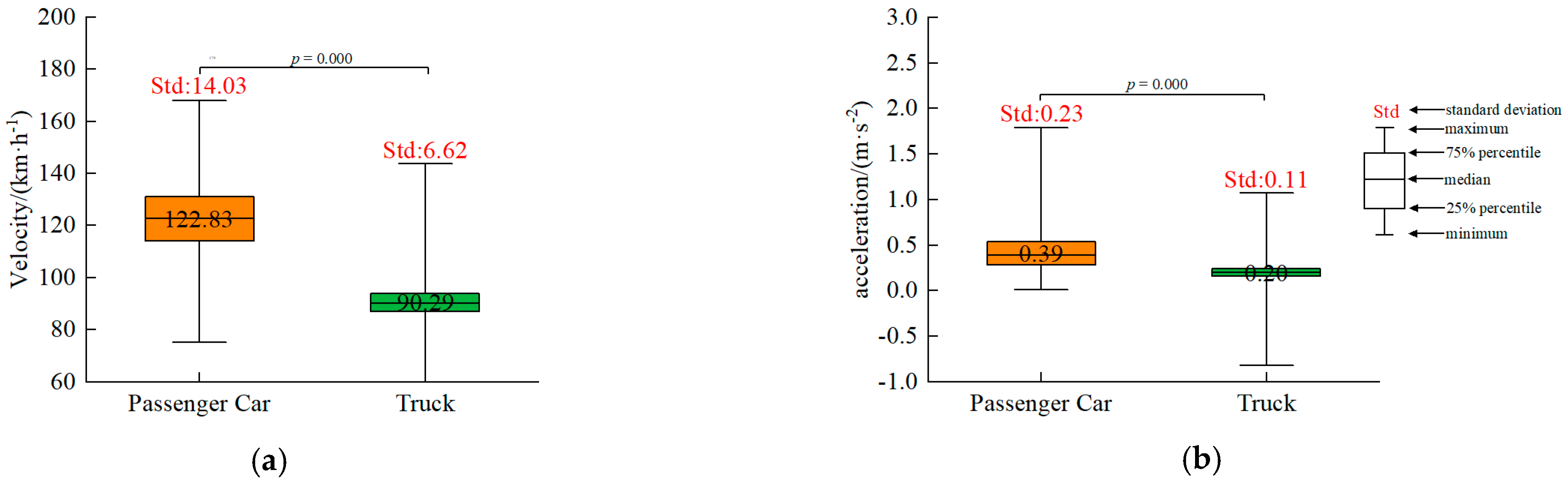
3.1. Free-Flow Condition

In the free-flow condition, speed and acceleration are selected for analyzing the driver behavior of passenger cars and trucks. The results are presented in Figure 1. The statistical indicator Kolmogorov–Smirnov (KS) is calculated for examining the difference of the results of two vehicle types. The KS results are also shown in Figure 1. A result of p < 0.05 indicates a significant difference between the two groups.

As shown in Figure 1, the median values of the speed and acceleration of passenger cars are both higher than those of trucks. The distribution of these two indicators for trucks is more concentrated than that of passenger cars. The 75th percentile value of the speed of passenger cars and trucks is 131.18 km·h⁻¹ and 93.85 km·h⁻¹, respectively. The KS results showed that passenger cars performed significantly differently compared to trucks on speed and acceleration due to their better flexibility and braking power.

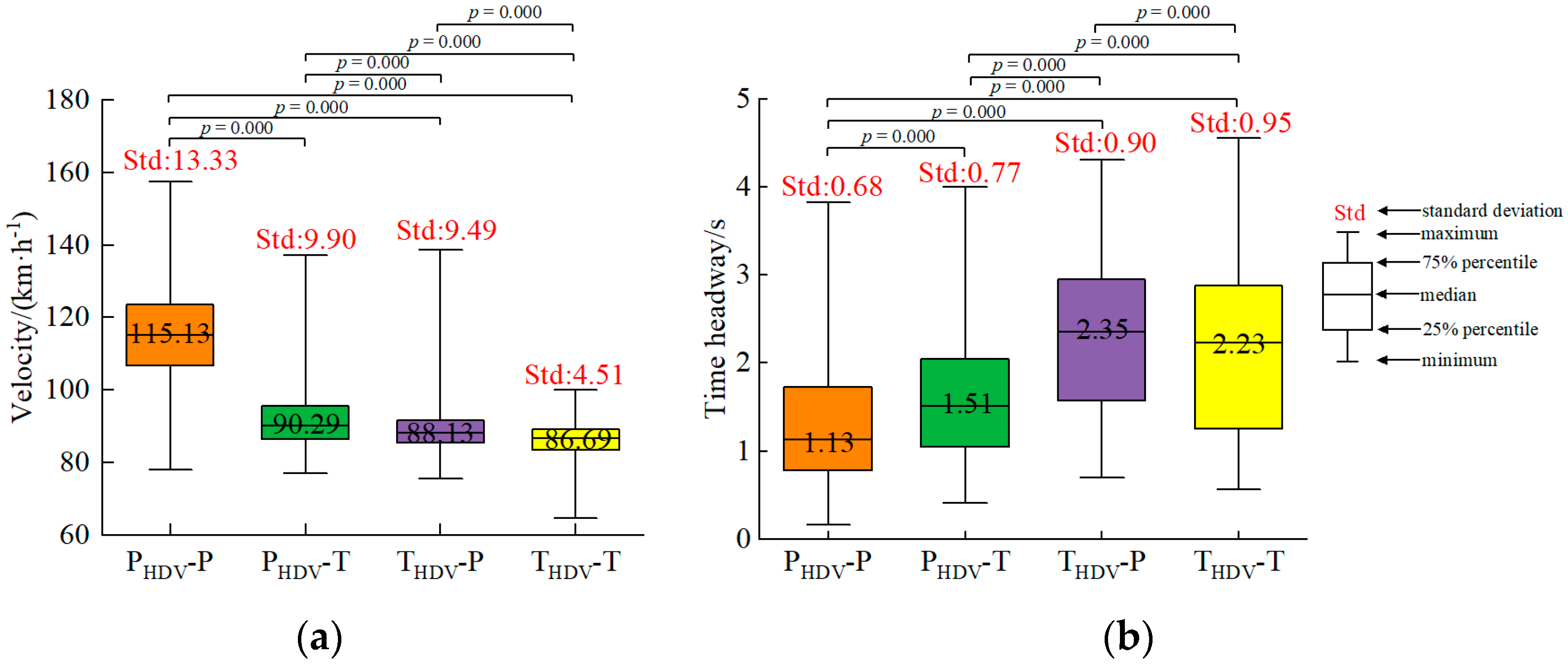
3.2. Car-Following Condition

Speed, acceleration, and time headway as the key indicators are selected for examining car-following driving behavior. The results of HDVs are shown in Figure 2.

Based on the results of Figure 2, which compares the average values of different car-following modes, the sequence of the speed is P_HDV-P > P_HDV-T > T_HDV-P > T_HDV-T, the same as the sequence of the acceleration, while the sequence of time headway is T_HDV-P > T_HDV-T > P_HDV-T > P_HDV-P. When an HDV passenger car is following another passenger car (P_HDV-P), the following passenger car is likely to choose high speed and short headway due to their strong and flexible control on the brake. While a truck cannot provide so much strong and flexible control on the brake due to its higher vehicle mass, the speed and acceleration of T-P mode is slower, and the headway is longer than that of P_HDV-P mode. On the other hand, when an HDV passenger car is following a truck (P_HDV-T), due to the caution towards trucks, the following speed is slower than that of P_HDV-P and the time headway is longer than that of P_HDV-P. Based on the weak control on the brake and the caution toward a truck, the speed of T_HDV-T is slowest in the four modes, and the time headway is further extended compared to P_HDV-T.

4. Optimization of Model Parameters Based on Following Combinations

This study updates the vehicle speed based on the acceleration model with the following framework. At time t (T = t), a speed v(t) is generated. At the same time, the current vehicle assesses the situation ahead and determines whether to accelerate or decelerate based on the speed of the leading vehicle. Then, a new speed is calculated based on the decision, and the acceleration model and time updates and the process moves on. The framework of the speed updating is illustrated in Figure 3.

To improve the accuracy of the model performance in highway conditions considering different vehicle types and automated levels, after examining the applicable environment and conditions of existing models, this study assumed that in the free-flow condition all vehicles are operated by the free-flow acceleration model regardless of vehicle type and automation level. And in the car-following condition, the HDV calibrates the parameters of the IDM model using empirical data based on different car-following combinations, while the AV applies the CACC model with parameters consistent with those obtained from real-world vehicle tests.

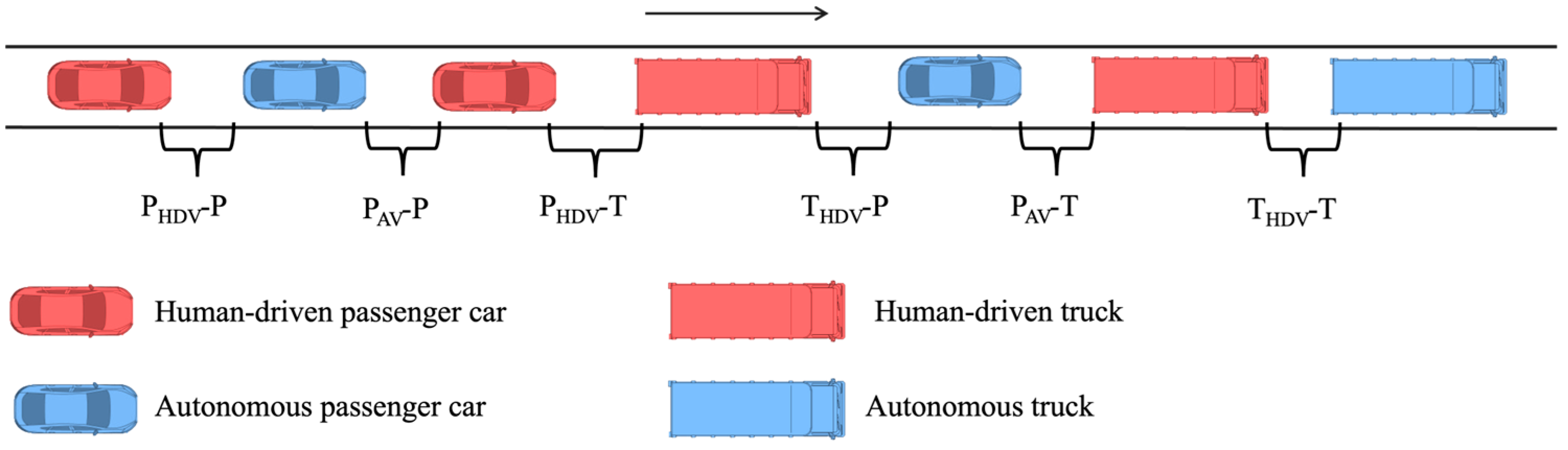
4.1. Scenario Introduction

This study examines the car-following behavior of P_HDV-P, P_HDV-T, T_HDV-P, T_HDV-T, P_AV-P, P_AV-T, T_AV-P and T_AV-T combinations in mixed traffic on a single-lane highway. A schematic diagram of the scenario is shown in Figure 4.

In this scenario, blue represents the HDV, while red denotes the AV. The notation for the modeling of the mixed traffic flow in a single-lane highway is shown in

Table 4. The notation of model parameters and variables.

Notion	Explanation
k	the coefficient of the free-flow acceleration model
vf	the desired speed of the vehicle
ai(t)	the acceleration of vehicle i at time t
vi(t)	the speed of vehicle i at time t
si(t)	the actual gap between vehicle i and its preceding vehicle at time t
δ	the free-flow acceleration exponent
s0	the minimum gap when the vehicle is stationary
h	the safe time headway
Δvi(t)	the speed difference between vehicle i and its preceding vehicle at time t
amax	the maximum acceleration of the vehicle
b	the maximum comfortable deceleration
kp	the coefficient of position error
kd	the coefficient of speed error

.

4.2. Model Introduction

4.2.1. Free-Flow Acceleration Model

It is assumed that the subject vehicle will maintain its acceleration until the desired speed under free-flow conditions is achieved. During this acceleration process, the vehicle will adjust its speed based on the difference in the current speed and desired speed. This study assumes that both HDVs and AVs are operated by the same free-flow acceleration model [28], and the model formula is shown in Equation (1).

$$a_i(t+1)=k(v_f-v_i(t))$$

(1)

The parameters k and v_f are required for calibration.

4.2.2. Car-Following Model for HDV—IDM Model

In the IDM model [9], the acceleration is a function of the desired speed, the distance to the vehicle ahead, and the safe time headway. The IDM acceleration model is illustrated by Equation (2):

$$a_i(t+1)=a_{\max }\left[1-{\left({\displaystyle \frac{v_i(t)}{v_f}}\right)}^{\delta }-\right.\left.{\left({\displaystyle \frac{s_0+v_i(t)h+\frac{v_i(t)\Delta v_i(t)}{2\sqrt{a_{\max }b}}}{s_i(t)}}\right)}^2\right]$$

(2)

The parameters δ, s₀, h, a_max, and b are required for calibration.

4.2.3. Car-Following Model for AV (Accelerating/Uniform Behavior)—CACC Model

An AV is assumed to be capable of obtaining the speed of the leading vehicle and providing good performance on driving stability. As a result, the AV will follow the leading vehicle with a speed that cannot exceed the speed of the leading vehicle. This is not the same as the IDM model: the CACC model is described by speed, and the formula is shown in Equation (3).

$$V_i(t+1)=v_i(t)+k_p(s_i(t)-v_i(t)h)+k_d(\Delta v_i(t)-a_i(t)h)$$

(3)

Based on real vehicle test results [28], the values of k_p and k_d are set to 0.45 and 0.0125, respectively.

4.2.4. Car-Following Model for AV (Decelerating)

The deceleration model is necessary in the simulation for preventing rear-end collisions. The AV activates the deceleration mode when the time headway drops below a predefined threshold. Currently, researchers mainly use the CACC model for realizing deceleration behavior (Equation (3)), with the difference between acceleration and deceleration behavior being reflected solely in the assignment of values to k_d, while k_p remains unchanged. Based on real vehicle test results, the values of k_p and k_d are set to 0.45 and 0.05 [28], respectively.

4.3. Parameter Optimization

4.3.1. Optimization Algorithm

Optimization algorithms aim to minimize the objective function, with commonly used methods including Newton’s method and the simulated annealing algorithm. Among them, simulated annealing is notable for its robust global search capability, which helps to avoid entrapment in local optima, particularly when dealing with high-dimensional-parameter spaces. Moreover, the algorithm features a simple structure and low sensitivity to initial values. By leveraging its probabilistic jump mechanism, SA can handle optimization problems involving both continuous and discrete variables, making it especially well-suited for calibrating complex nonlinear systems. Therefore, the simulated annealing algorithm is adopted in this study for the parameter calibration of the car-following model.

The execution process of the simulated annealing algorithm is as follows: an initial solution is randomly generated, and temperature parameters are initialized. A new solution is then produced using a neighborhood function, and the change in the objective function value is computed. Based on the Metropolis criterion, the new solution is either accepted or rejected. Subsequently, the temperature is decreased according to a predefined cooling schedule. The iteration continues until a convergence condition is met, upon which the optimal solution is output. In the early stage with high temperature, the algorithm performs a broad global search; as the temperature decreases, it gradually transitions to a more refined local search.

In this study, the simulated annealing algorithm is implemented on the MATLAB (R2023b) platform with the following parameters: an initial temperature of 1000, a cooling coefficient of 0.95, a termination temperature of 10⁻⁶, and 100 iterations per temperature level. Considering the inherent stochastic nature of the algorithm, each calibration process is repeated eight times to ensure a thorough exploration of the solution space. The result with the lowest objective function value among the eight runs is selected as the final calibrated parameter set.

4.3.2. Parameter Calibration Results

The calibration was conducted based on the HighD dataset. Various traffic flow parameters were firstly collected from the dataset, including, the speed, acceleration, and distance headway of the following vehicles and the speed of the leading vehicles based on the summary of Section 4.2. Then, the IDM model described in Section 4.2 was fitted by applying simulated annealing method. To facilitate a comparison with the parameters calibrated from empirical data [24,28], the calibration results are categorized into the Tested Data Model (TM) and Empirical Data Model (EM), as shown in

Table 5. Calibration results of driving behavior model parameters based on tested and empirical data.

Model	Parameters	TM				EM
		Passenger Car		Truck		Passenger Car		Truck
Free-flow acceleration modeling	k	0.032		0.028		0.4
	vf/(km·h−1)	131.18		93.85		120		100
Model	Parameters	TM				EM
		PHDV-P	PHDV-T	THDV-P	THDV-T	PHDV-P	PHDV-T	THDV-P	THDV-T
IDM	amax/(m·s−2)	0.24	0.13	0.44	0.03	1
	vf/(km·h−1)	131.18		93.85		120		100
	s0/m	2.93	1.39	2.95	1.48	2
	b/(m·s−2)	3.60	1.73	0.57	1.00	2
	h/s	0.16	0.40	1.05	3.08	1.5		2
	δ	8.41	2.71	0.77	2.56	4

.

4.3.3. Model Validation Based on TM and EM Parameters

To assess the accuracy of the parameter calibration results, the free-flow acceleration model and the IDM are verified by inputting the TM and EM parameter values, respectively. The statistical error indices including Mean Absolute Percentage Error (MAPE), Mean Absolute Error (MAE), and Root Mean Square Error (RMSE) were calculated for the validation. The comparison results are presented in Figure 5 and Figure 6.

Figure 5 shows the validation results of the free-flow acceleration model. It is found that the statistical error values are significantly decreased under the condition of applying TM parameter values regardless of vehicle type. Based on the data collection, the free-flow speed of passenger cars was increased from 120 km·h⁻¹ to 131.18 km·h⁻¹, and this value of trucks was reduced from 100 km·h⁻¹ to 93.85 km·h⁻¹. This adjustment ensures that the model performed acceleration behavior more reliably; therefore, the error is decreased.

As shown in Figure 6, the models calibrated with TM parameters exhibit significant improvements in four car-following combinations—P_HDV-P, P_HDV-T, T_HDV-P, and T_HDV-T—with simulation accuracy increases of 90.40%, 81.75%, 58.29%, and 91.77%, respectively. This demonstrated that the model calibrated by the TM parameters can simulate the car-following behaviors more accurately.

5. Optimization Numerical Simulation

5.1. Overview of the Simulation Environment

The simulation platform MATLAB (R2023b) is applied here for establishing the simulation environment. Only car-following behavior was considered in this study; thus, a single-lane highway with a length of 500 m is designed in the simulation. Fifteen vehicles are assigned to travel on the road. The simulation is run based on the cellular automata theory, and the road is divided into multiple cells with a single cell length of 1 cm. The number of cells occupied by a vehicle is dependent on its length; for example, a passenger car with 5 m occupies 500 cells. The proportions of AVs and trucks in the traffic flow are defined as p and q, respectively; then, the proportions of HDVs and passenger cars are calculated as (1−p) and (1−q). Thus, the probability of T_HDV, P_HDV, T_AV, and P_AV can be calculated as (1−p) × q, (1−p) × (1−q), p × q, and p × (1−q), in the order listed. It is assumed that the range of p is from 0 to 100% with an interval of 20%, and the value of q follows the same assumption. Thus, scenarios will be examined in the simulation. At the beginning of the simulation, the vehicles are assigned with the same interval of distance, and random slowing is not considered either for HDVs or AVs in the simulation. The simulation runs for 1500 s with a time step of 0.05 s for data collection. The data during 1000–1500 s are collected as the simulation results considering the stability of the traffic flow. Additionally, the simulation is run 10 times for each scenario to minimize the influence of randomness. The average results of these 10 simulations are calculated as the final results for analysis.

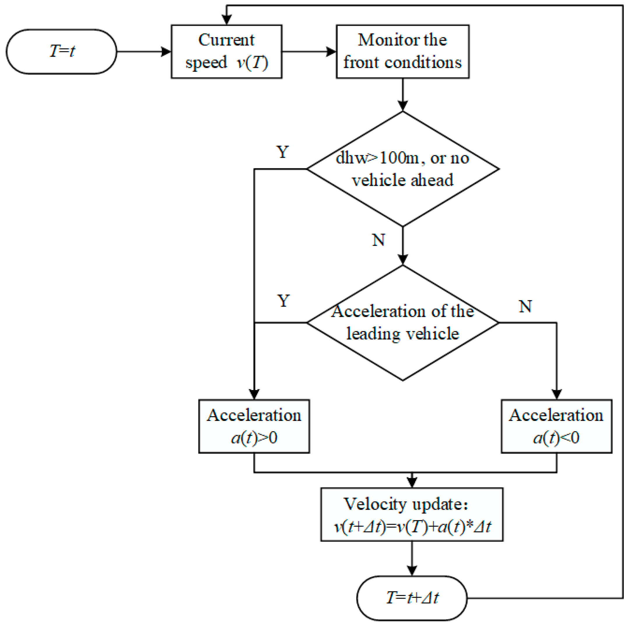
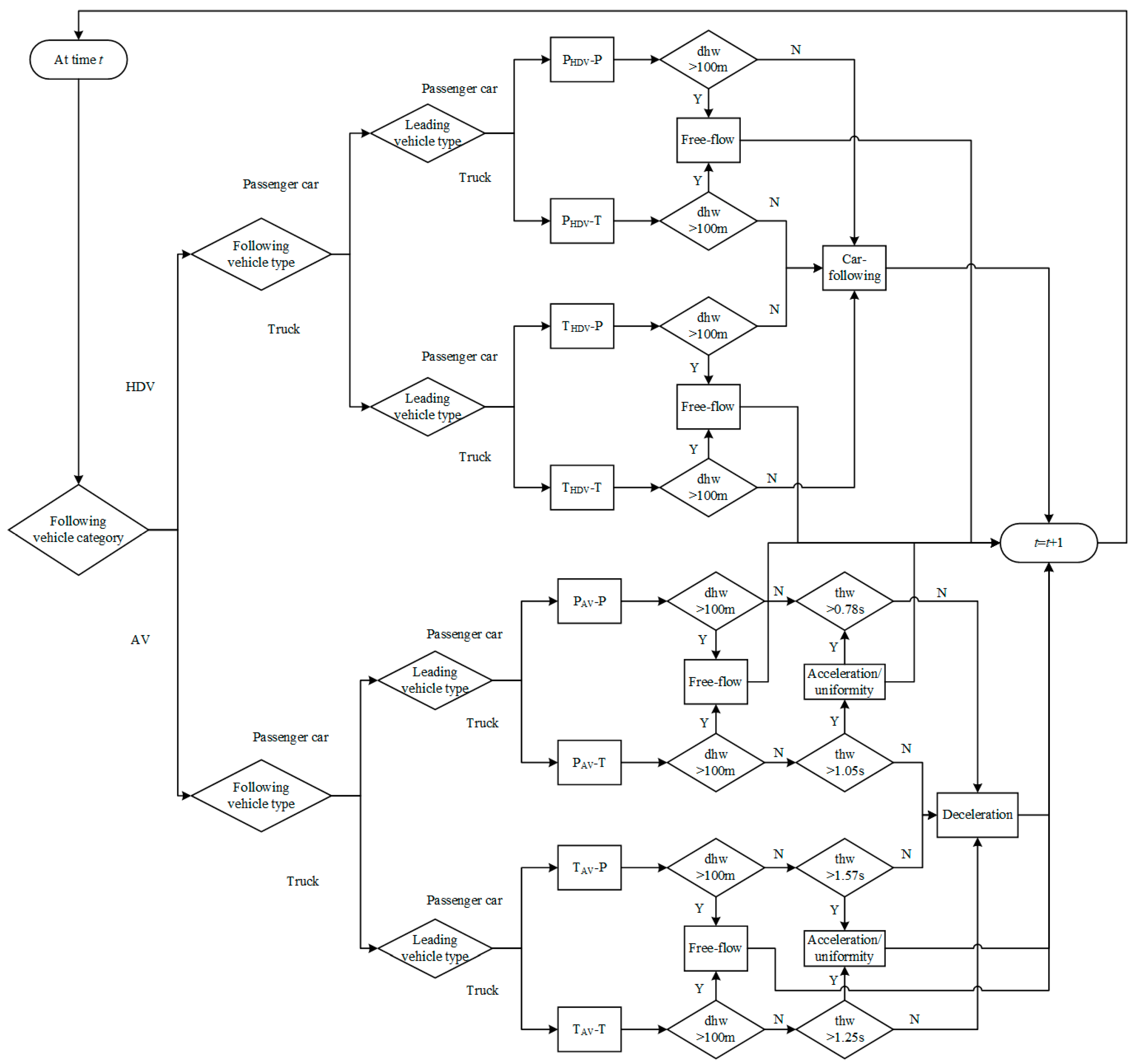
5.2. Overview Threshold for Decision of Car-Following Behavior

The decision of car-following behavior is firstly made by the distance between two vehicles, which is from the definition of “car-following behavior” (<100 m). Then, the following headway is assigned based on the car-following combination mode of the subject vehicle and the front vehicle. The framework of this decision-making process is shown in Figure 7.

As shown in Figure 7, if the subject vehicle is an HDV, its driving behavior is classified as either free-flow or car-following. Conversely, when the subject vehicle is an AV, the behavior is classified into free-flow, acceleration/uniform mode, and deceleration. The threshold value for distinguishing between acceleration/uniform mode and deceleration for AVs is derived from the 25th percentile of the observed time headways in the AV car-following dataset. This is based on the assumption that vehicles tend to decelerate when the headway becomes relatively short, indicating a reduced safety margin. Therefore, 25% is used to represent a critical headway below which deceleration is more likely to occur. Specifically, the thresholds for the P_AV-P, P_AV-T, T_AV-P, and T_AV-T combinations are 0.78 s, 1.05 s, 1.57 s, and 1.25 s, respectively. This means that when headway is lower than the threshold value, the following vehicle (subject vehicle) will choose to decelerate.

6. Optimization Results and Analysis

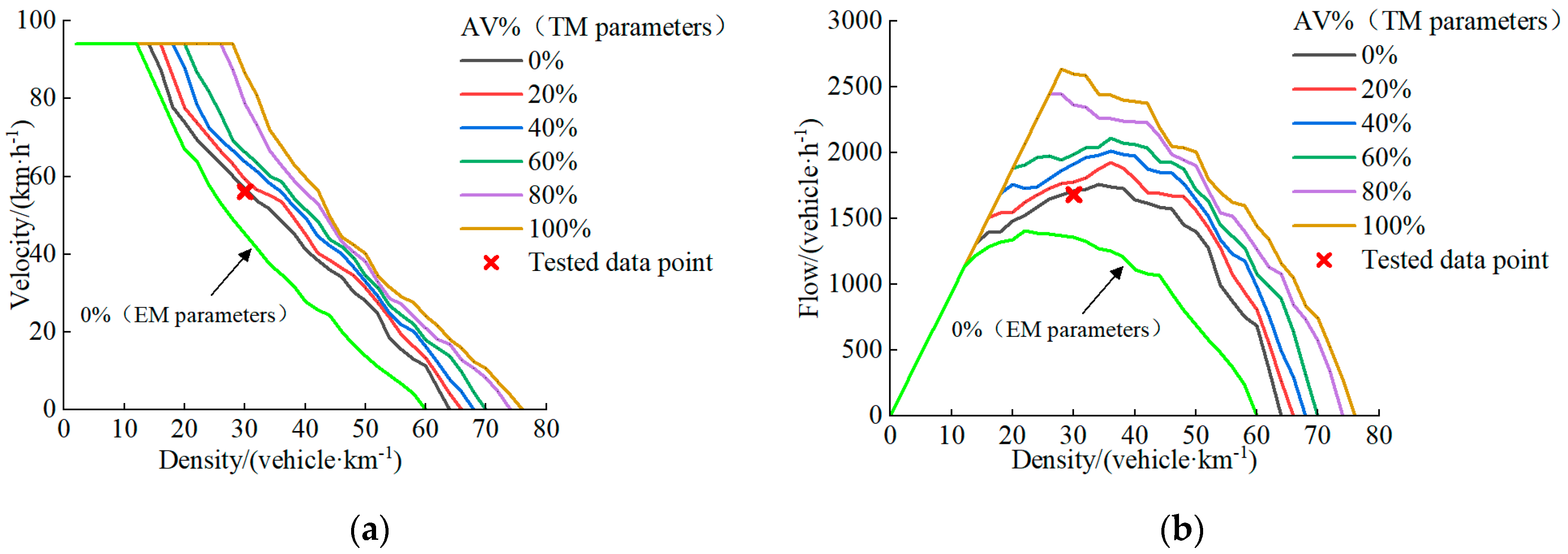
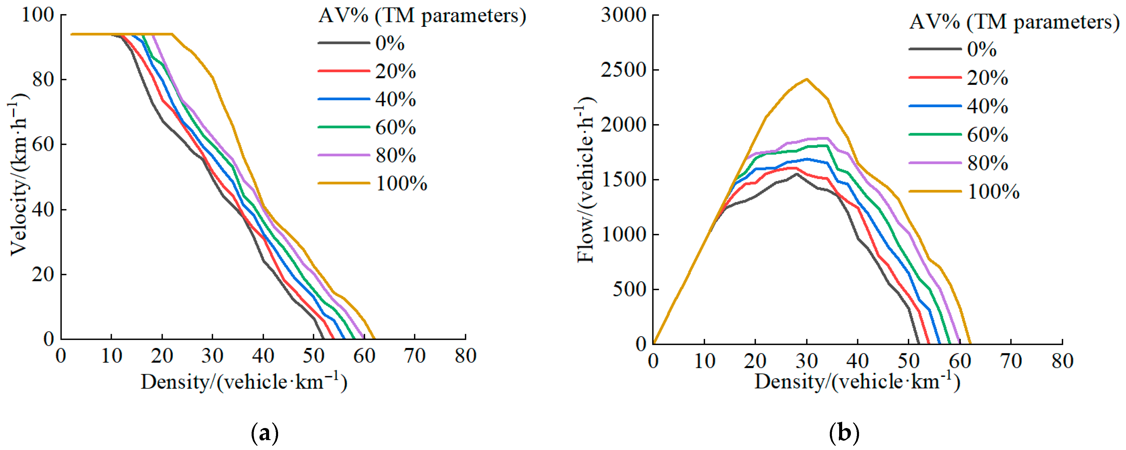
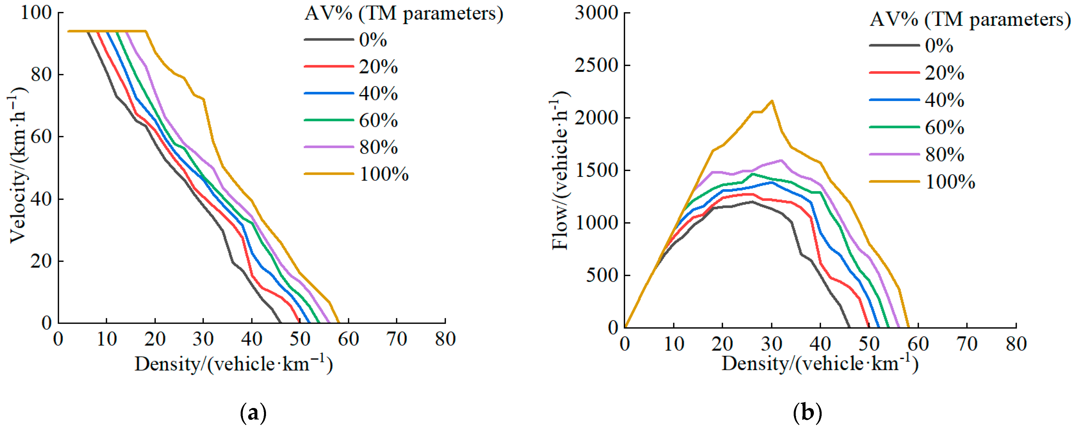
6.1. Traffic Flow Characteristics at Different Levels of T% and AV%

Figure 8, Figure 9 and Figure 10 present the results of speed–density (series (a)) and flow–density (series (b)) under the different conditions of T% and AV%. The conditions of T% = 20%, 60%, and 100% were chosen as the examples.

T% = 20% is observed based on the empirical dataset; thus, AV = 0% under this condition should represent the real situation of the traffic flow. As shown in Figure 8, the observed data points fall precisely on the TM parameter curve, not on the EM parameter curve. This demonstrated that the accuracy of the models with TM parameter is much higher than that of EM parameter. Specifically, at a traffic density of 30 vehicles·km⁻¹, the observed average speed is 56.12 km·h⁻¹. The TM model simulation with AV% = 0% yields a speed of 57.05 km·h⁻¹, with a minor deviation of 0.93 km·h⁻¹. In contrast, the EM model predicts a significantly lower speed of 45.28 km·h⁻¹, resulting in a deviation of 10.84 km·h⁻¹. It is suggested that the simulation model is established based on real conditions.

As shown in Figure 8 and Figure 10, both speed and traffic flow are influenced by the proportions of AV% and T%, as well as by traffic density. In the condition of each T% level, speed increases with AV% increasing, reaching its maximum at AV% = 100%. Conversely, for any AV% level, speed decreases when density is increased, consistent with fundamental traffic flow characteristics. It can be also determined that the part of the speed curve parallel to the horizontal axis represents the under-saturated situation. As AV% is increased, the critical density of under-saturated to over-saturated is increased, indicating that a higher proportion of AVs causes traffic to enter a car-following state at higher densities. However, for any AV% level, speed decreases when T% is increased. Similarly, traffic flow exhibits a typical concave trend: it initially increases with density and subsequently declines. At any given T% level, a higher AV% leads to an increase in maximum traffic flow. In contrast, increasing T% reduces the road capacity, reflecting the negative impact of a higher truck proportion on overall traffic performance.

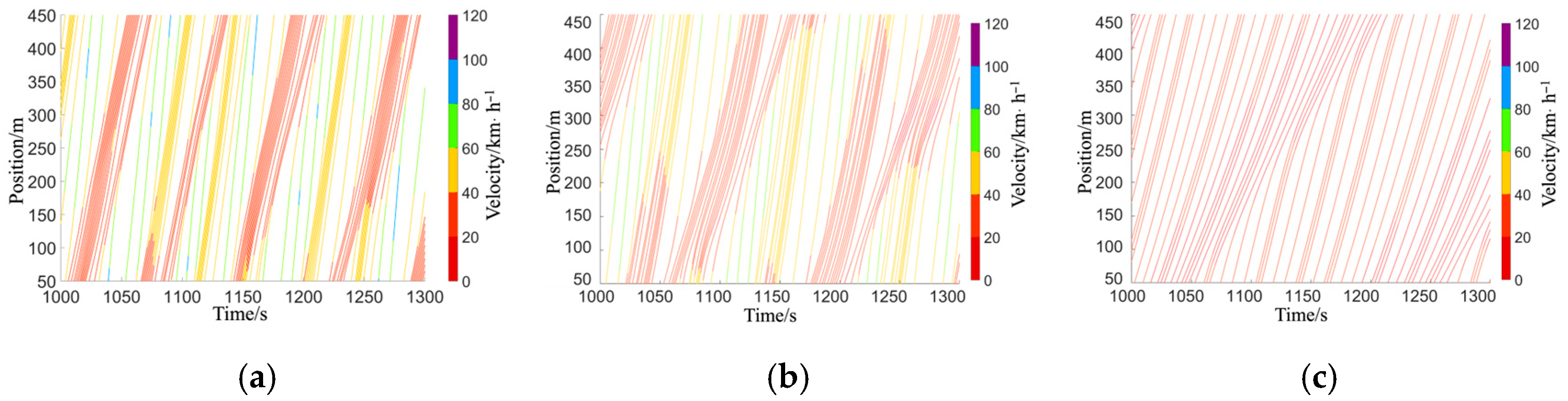
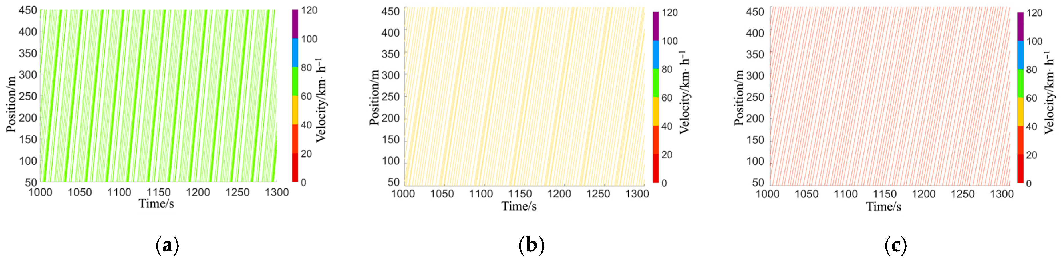
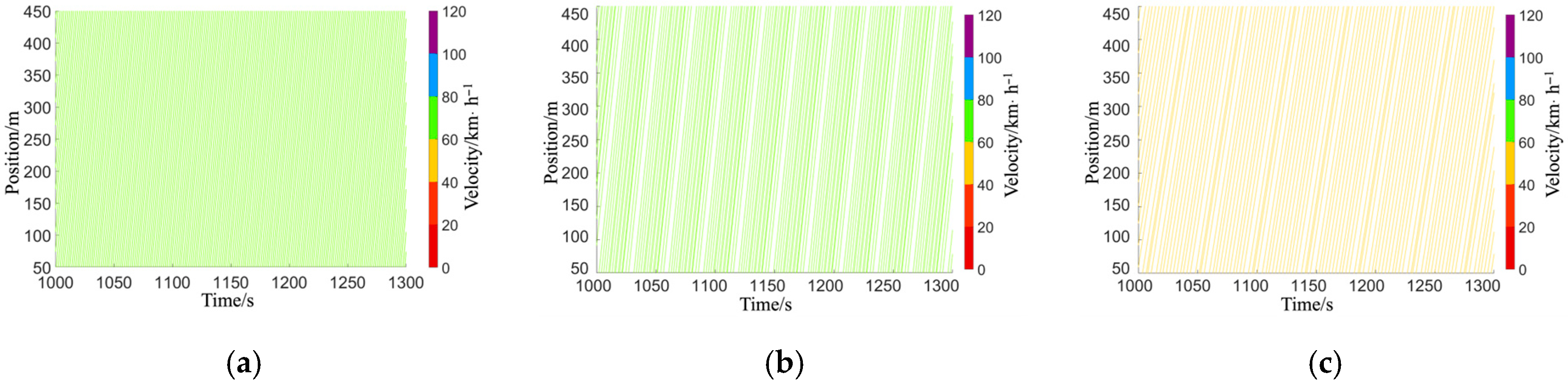
6.2. Time–Space Results at Different T% and AV%

Figure 11, Figure 12 and Figure 13 present the time–space plots at different AV% and T% levels under the condition of a fixed density of 30 vehicle·km⁻¹

As shown in Figure 11, Figure 12 and Figure 13, increasing T% results in a marked reduction in vehicle speed and a greater curvature in vehicle trajectories, indicating enhanced speed fluctuations and their propagation throughout the traffic flow. Specifically, at AV% = 0%, when T% rises from 20% to 80%, these disturbances become more pronounced, evident in the abrupt speed changes and increased trajectory fluctuations. At T% = 80%, the frequency and reach of these fluctuations grow, underscoring how a higher truck percentage degrades traffic flow efficiency and escalates system instability. In contrast, as AV% increases, vehicle trajectories smooth out and speed variations lessen, promoting greater operational stability, even under high T% conditions. For example, at T% = 80% and AV% = 80%, the minimal trajectory fluctuations and near-stable traffic flow suggest that autonomous vehicles help mitigate the disruptions caused by the higher truck proportion, ultimately enhancing both stability and performance in mixed traffic flow.

The observed speed fluctuations have direct consequences for vehicular emissions, as quantified by the VT-Micro model [29]. This model establishes a logarithmic relationship between emission rates and instantaneous vehicle dynamics:

$$In(MO{E}_e)={\displaystyle \sum _{k=0}^3{\displaystyle \sum _{l=0}^3{K}_{k,l}}}{v}_i{(t)}^k{a}_i{(t)}^l$$

(4)

where MOE_e represents the rate of fuel consumption or emission (e.g., carbon monoxide CO, hydrocarbon HC, etc.) and K_k,l are the emission coefficients for the k-th velocity and l-th acceleration state.

According to this model, emissions increase when acceleration and deceleration are frequent, as seen in high T% scenarios. As vehicle speed fluctuations grow, these patterns lead to inefficient driving and higher emissions. In contrast, when the AV% rises, the traffic flow stabilizes, reducing the frequency of acceleration and deceleration events, leading to smoother vehicle trajectories.

6.3. Mean Speed Heatmaps Under Varying T% and AV% Conditions

Figure 14 presents the mean speed heatmaps for different AV% and T% combinations with a fixed vehicle density of 30 vehicles·km⁻¹. The color variations correspond to different speed levels. The percentage value under the speed value in each blank represents the changing rate, which compares the speed in the current condition to the P_HDV = 100% condition.

As shown in Figure 14, in each AV% level, the average speed decreases as T% increases. However, when AV% = 100%, the speed in the condition T% = 100% is higher than that of T% = 80%. This can be explained by the fact that with both AV% and T% assigned to 100%, all vehicles are autonomous trucks. This makes the traffic flow shift from a mixed situation to a uniform composition, which reduces the complexity of the traffic flow. This change allows AV trucks to increase the average vehicle speed more effectively.

In each level of T%, an increase in the AV% brings an improvement in speed. As AV% increases from 0% to 80%, the rate of increase in average speed is gradual, but from 80% to 100%, the increase in average speed becomes sharper. This indicates that when AVs are 100% occupied, the average vehicle speed can be significantly enhanced, efficiently improving the operational performance of the traffic flow.

Finally, the improvement in speed from increasing AVs cannot cover the reduction in speed by truck input under the same percentage value. For example, the speed improvement of increasing AVs by 20% is smaller than that of the speed reduction of trucks’ 20% input. This result suggests that the influence of trucks on speed is more significant than AVs.

7. Discussion

(1)

This study analyzes driving behaviors, including the speed and acceleration of cars and trucks, under various traffic flow conditions using the HighD dataset, specifically focusing on the free-flow and follow-me datasets. Additionally, within the following dataset, which includes both HDVs and AVs, the following combinations are categorized into eight types: P_HDV-P, P_HDV-T, T_HDV-P, T_HDV-T, P_AV-P, P_AV-T, T_AV-P, and T_AV-T. The analysis of driving behaviors, such as speed, acceleration, and headway time, revealed notable differences in vehicle conditions across various following combinations.

(2)

This study presents the calibration of the following behavior model parameters using the simulated annealing method with measured data. The calibrated parameter model was subsequently compared with the empirical model. The results show that the parameter optimization method, which accounts for different follower combinations, enhances the accuracy of the model in capturing the driving behavior characteristics of various vehicle type and category combinations within the traffic flow. Specifically, the calibrated model achieves an average improvement of 85.31% in MAPE, 79.19% in MAE, and 77.02% in RMSE compared to the empirical model. Consequently, it can be concluded that this method significantly improves the accuracy of traffic flow predictions.

(3)

This study developed a cellular automaton model to simulate mixed passenger and goods traffic flow in both AV and HDV environments. The results show that AV% and T% significantly influence the efficiency and stability of traffic flow. Increasing the AV% improves road capacity, enhances traffic flow stability, and raises the overall average speed. As AV penetration increases, traffic volume rises by 50%. In contrast, a higher T% reduces traffic flow stability and lowers the average speed. In the case of full truck penetration, the average speed decreases by 75.37%. However, traffic stability at T% = 100% is more favorable than in mixed passenger and freight scenarios. Increased stability from higher AV penetration helps reduce fluctuations in traffic speed, leading to lower emissions by minimizing unnecessary acceleration and deceleration. In contrast, higher truck percentages tend to degrade traffic flow, leading to higher emissions.

(4)

This study primarily focuses on car-following behavior in a single-lane highway scenario, assuming that automated vehicles (AVs) strictly follow the CACC model during acceleration and deceleration, while neglecting real-world factors such as communication delays, perception errors, and control execution deviations. The type of lead vehicle (AV or HDV) and the vehicle connectivity environment are also not considered. Future research will build upon this model by incorporating more complex vehicle interactions, such as lane-changing behavior, and exploring its application in diverse driving environments like highway weaving zones.

References

1. Bansal, P.; Kockelman, M.K. Forecasting Americans’ Long-Term Adoption of Connected and Autonomous Vehicle Technologies. Transp. Res. Part A 2017, 95, 49–63. [Google Scholar] [CrossRef]
2. Gipps, P.G. A Behavioural Car-Following Model for Computer Simulation. Transp. Res. Part B Methodol. 1981, 15, 105–111. [Google Scholar] [CrossRef]
3. Jiang, R.; Wu, Q.; Zhu, Z. Full Velocity Difference Model for a Car-Following Theory. Phys. Rev. E 2001, 64, 017101. [Google Scholar] [CrossRef]
4. Bando, M.; Hasebe, K.; Nakayama, A.; Shibata, A.; Sugiyama, Y. Dynamical Model of Traffic Congestion and Numerical Simulation. Phys. Rev. E 1995, 51, 1035–1042. [Google Scholar] [CrossRef]
5. Helbing, D.; Tilch, B. Generalized Force Model of Traffic Dynamics. Phys. Rev. E 1998, 58, 133–138. [Google Scholar] [CrossRef]
6. Nagel, K.; Schreckenberg, M. A Cellular Automaton Model for Freeway Traffic. J. Phys. I 1992, 2, 2221–2229. [Google Scholar] [CrossRef]
7. Takayasu, M.; Takayasu, H. 1/f Noise in a traffic model. Fractals 1993, 04, 860–866. [Google Scholar] [CrossRef]
8. Barlovic, R.; Santen, L.; Schadschneider, A.; Schreckenberg, M. Metastable States in Cellular Automata for Traffic Flow. Eur. Phys. J. B Condens. Matter Complex Syst. 1998, 5, 793–800. [Google Scholar] [CrossRef]
9. Treiber, M.; Hennecke, A.; Helbing, D. Congested Traffic States in Empirical Observations and Microscopic Simulations. Phys. Rev. E 2000, 62, 1805–1824. [Google Scholar] [CrossRef]
10. Milanés, V.; Shladover, S.E. Modeling Cooperative and Autonomous Adaptive Cruise Control Dynamic Responses Using Experimental Data. Transp. Res. Part C Emerg. Technol. 2014, 48, 285–300. [Google Scholar] [CrossRef]
11. Jia, B.; Jiang, R.; Gao, Z.-Y.; Zhao, X.-M. The effect of mixed vehicles on traffic flow in two lane cellular automata model. Int. J. Mod. Phys. C 2005, 16, 1617–1627. [Google Scholar] [CrossRef]
12. Ebersbach, A.; Schneider, J.; Morgenstern, I.; Hammwöhner, R. The Influence of Truck on Traffic Flow: An Investigation on the Nagel-Schreckenber-Model. Int. J. Mod. Phys. C 2000, 11, 837–842. [Google Scholar] [CrossRef]
13. Meng, Q.; Weng, J. An Improved Cellular Automata Model for Heterogeneous Work Zone Traffic. Transp. Res. Part C Emerg. Technol. 2011, 19, 1263–1275. [Google Scholar] [CrossRef]
14. Moridpour, S.; Mazloumi, E.; Mesbah, M. Impact of Heavy Vehicles on Surrounding Traffic Characteristics. J. Adv. Transp. 2015, 49, 535–552. [Google Scholar] [CrossRef]
15. Dewen, K.; Xiucheng, G.; Bo, Y. Analyzing the Impact of Trucks on Traffic Flow Based on an Improved Cellular Automaton Model. Discret. Dyn. Nat. Soc. 2016, 2016, 1–14. [Google Scholar]
16. Yang, D.; Qiu, X.; Yu, D.; Sun, R.; Pu, Y. A Cellular Automata Model for Car–Truck Heterogeneous Traffic Flow Considering the Car–Truck Following Combination Effect. Phys. A Stat. Mech. Appl. 2015, 424, 62–72. [Google Scholar] [CrossRef]
17. Baikejuli, M.; Shi, J. A Cellular Automata Model for Car–Truck Heterogeneous Traffic Flow Considering Drivers’ Risky Driving Behaviors. Int. J. Mod. Phys. C 2023, 34, 2350154. [Google Scholar] [CrossRef]
18. Liu, L.; Zhu, L.; Yang, D. Modeling and Simulation of the Car-Truck Heterogeneous Traffic Flow Based on a Nonlinear Car-Following Model. Appl. Math. Comput. 2016, 273, 706–717. [Google Scholar] [CrossRef]
19. Yunze, W.; Ranran, X.; Ke, Z. A Car-Following Model for Mixed Traffic Flows in Intelligent Connected Vehicle Environment Considering Driver Response Characteristics. Sustainability 2022, 14, 11010. [Google Scholar] [CrossRef]
20. Liu, H.; Kan, X.; Shladover, S.E.; Lu, X.-Y.; Ferlis, R.E. Modeling Impacts of Cooperative Adaptive Cruise Control on Mixed Traffic Flow in Multi-Lane Freeway Facilities. Transp. Res. Part C Emerg. Technol. 2018, 95, 261–279. [Google Scholar] [CrossRef]
21. Xie, H.; Ren, Q.; Lei, Z. Influence of Lane-Changing Behavior on Traffic Flow Velocity in Mixed Traffic Environment. J. Adv. Transp. 2022, 1, 1–26. [Google Scholar] [CrossRef]
22. Zhang, W.; Liu, J.; Xie, L.; Ding, H. Analysis on the characteristics of traffic flow in expressway weaving area under mixed connected and autonomous environment. J. Southeast Univ. (Nat. Sci. Ed.) 2023, 53, 156–164. [Google Scholar]
23. Zhang, W.; Liu, J.; Xie, L.; Ding, H. Lane-Changing Model of Autonomous Vehicle in Weaving Area of Expressway in Intelligent and Connected Mixed Environment. J. Jinlin Univ. (Eng. Technol. Ed.) 2023, 54, 469–477. [Google Scholar] [CrossRef]
24. Wu, D.; Chen, R. Characteristics of passenger-cargo mixed traffic flow in intelligent network and agglomeration lane-change strategy. J. Jilin Univ. (Eng. Technol. Ed.) 2024, 1–9. [Google Scholar] [CrossRef]
25. Wang, Y.; Gan, H.; Wang, K.; Cheng, Z. Dedicated lane management and control strategy of intelligent heavy trucks based on cellular automata. Univ. Shanghai Sci. Technol. 2024, 47, 100–107. [Google Scholar] [CrossRef]
26. Zhou, J.; He, Y.; Tian, J. Speed Characteristic Analysis Based on NGSIM Trajectory Data. Technol. Econ. Areas Commun. 2019, 21, 45–48+61. [Google Scholar]
27. Gu, H. Research on Freeway Car-Following Modeling and Simulation in Connected Vehicle Environment. Ph.D. Thesis, Southeast University, Nanjing, China, 2017. [Google Scholar]
28. Guo, X.; Xiao, Z.; Zhang, Y.; Zhang, Y.; Xu, P. Variable Speed Limit Control Method in Work Zone Area of Eight-lane Highway Considering Effects of Connected Automated Vehicles. J. Southeast Univ. (Nat. Sci. Ed.) 2024, 54, 353–359. [Google Scholar]
29. Wu, S.; Zou, Y.; Liu, D.; Chen, X.; Wang, Y. Investigating Traffic Characteristics at Freeway Merging Areas in Heterogeneous Mixed-Flow Environments. Sustainability 2025, 17, 2282. [Google Scholar] [CrossRef]
Figure 1. Driving behavior results for passenger cars and trucks under the free-flow condition: (a) speed; (b) acceleration.
Sustainability 17 06450 g001
Figure 2. Driving behavioral results with different HDV car-following combinations: (a) speed; (b) time headway.
Sustainability 17 06450 g002
Figure 3. Vehicle speed update flowchart.
Sustainability 17 06450 g003
Figure 4. Car-following schematic in mixed traffic flow.
Sustainability 17 06450 g004
Figure 5. Free-flow acceleration model comparison results: (a) passenger car; (b) truck.
Sustainability 17 06450 g005
Figure 6. IDM model comparison results: (a) PHDV-P; (b) PHDV-T; (c) THDV-P; (d) THDV-T.
Sustainability 17 06450 g006
Figure 7. Vehicle driving behavior judgment flowchart.
Sustainability 17 06450 g007
Figure 8. Characteristics of the mixed traffic flow at different AV% (T% = 20%): (a) speed-density; (b) flow-density.
Sustainability 17 06450 g008
Figure 9. Characteristics of the mixed traffic flow at different AV% (T% = 60%): (a) speed-density; (b) flow-density.
Sustainability 17 06450 g009
Figure 10. Characteristics of the mixed traffic flow at different AV% (T% = 80%): (a) speed-density; (b) flow-density.
Sustainability 17 06450 g010
Figure 11. The time–space plots under different T% (AV% = 0%): (a) T% = 20%; (b) T% = 60%; (c) T% = 80%.
Sustainability 17 06450 g011
Figure 12. The time–space plots under different T% (AV% = 60%): (a) T% = 20%; (b) T% = 60%; (c) T% = 80%.
Sustainability 17 06450 g012
Figure 13. The time–space plots under different T% (AV% = 80%): (a) T% = 20%; (b) T% = 60%; (c) T% = 80%.
Sustainability 17 06450 g013
Figure 14. Mean speed thermograms at different T% and AV%.
Sustainability 17 06450 g014