Carbon-Aware Spatio-Temporal Workload Shifting in Edge–Cloud Environments: A Review and Novel Algorithm

Abstract

Due to its rising carbon footprint, new paradigms for carbon-efficient computing are needed. For distributed computing systems, one option is to shift computing loads in space or time to take advantage of low-carbon electricity, a paradigm known as carbon-aware computing. We present a literature review of carbon-aware scheduling techniques, which shows that most of the literature carried out either spatial or temporal shifting but not both. Of the 28 analyzed studies, 11 considered both spatial and temporal shifting, and only 2 developed a combined optimization algorithm. Additionally, existing approaches typically focus on operational electricity alone. With the growing decarbonization of electricity, however, device production (which involves various industrial processes and cannot be easily decarbonized) is bound to become more relevant and needs to be considered. We thus suggest a novel spatio-temporal scheduling algorithm for cloud and edge computing. Our algorithm performs simultaneous spatio-temporal shifting while taking into consideration both device production and operation. As temporal shifting requires forecasts of future workloads, we also put forward a workload predictor. Although not fully implemented yet, we bring various theoretical arguments in support of our proposed algorithm.

1. Introduction

Driven by trends such as AI, IoT, streaming, and the move towards cloud and edge computing, computing has a rising energy demand [1,2]. This brings a dilemma: on one side, given the environmental and societal benefits that computing induces, the field is bound (and arguably even required) to grow. On the other side, however, as this growth can most likely no longer be outweighed by hardware efficiency gains, new paradigms and strategies for an energy- and carbon-efficient computing need to be devised. Strategies are manifold and take different approaches, such as deploying energy-efficient computing to decrease the overall energy requirements [3,4,5] or the use of low-carbon electricity to decrease the carbon footprint of computation. This latter strategy is often achieved from a market-based perspective [6] by either generating on-site renewable energy, via power-purchasing agreements (PPAs), or through guarantees of origin (GOs). This approach, while in principle meaningful, has also been criticized for enabling the double-counting of green electricity, which makes the overall carbon emissions from electricity appear smaller than they actually are [7].

Green Cloud Computing (GCC) suggests a set of approaches to mitigate the environmental impact of cloud computing [8]. One of those decreases the carbon footprint according to what is called the “location-based approach” (i.e., it accounts for the average carbon intensity of the grid mix at the location and time of usage). Also called “carbon-aware computing” [9], its principle is to shift workloads in space and/or time to take advantage of lower-carbon electricity, whenever and wherever it is available. The corresponding, “carbon-aware workload scheduling” can be described as an intelligent arrangement and execution of computational tasks such that the carbon footprint associated with their operation is minimized. While traditional scheduling methods focus on performance metrics like speed and computational efficiency, carbon-aware scheduling incorporates environmental considerations, where tasks are prioritized based on the availability of renewable energy sources indicated by the varying carbon intensity (CI) of electricity.

In the landscape of distributed systems, Kubernetes [10] emerges as a pivotal tool in enabling carbon-aware computing, particularly suited for orchestrating containerized applications across distributed cloud and edge environments. It automates the deployment, scaling, and management of applications, aligning well with the need for dynamic resource allocation based on environmental impact. Kubernetes can further be extended to support advanced scheduling algorithms that integrate carbon intensity data.

In this context, the contributions of this paper are fourfold: (i) It provides a literature review of existing carbon-aware scheduling techniques (in either time or location). (ii) Building on the insights from this review, it suggests a novel spatio-temporal scheduling algorithm for cloud and edge computing. Unlike our proposal, most of the literature carries out either spatial or temporal shifting but not both. Additionally, the focus typically lies on the operational electricity alone. Device production, however, involves various industrial processes and cannot be easily decarbonized, and for smaller devices, it is already the main source of environmental impact [11]. With the growing decarbonization of operational electricity, device production is bound to become more relevant for larger devices as well. Our third contribution is thus to (iii) introduce principles to account for the carbon embodied during production and to reflect it in the algorithm. Finally, as will be argued later in the paper, a prerequisite for temporal shifting are forecasts of both carbon intensity of electricity and of workloads. Carbon intensity predictions inform whether shifting into the future is meaningful; load predictions inform whether it is possible (i.e., whether there will likely be free capacity). While for the former we consult external sources, contribution (iv) is a workload predictor. Overall, and although parts of the algorithm implementation are still ongoing (the workload predictor being already available on GitHub [12]), we bring various theoretical arguments in support of our proposal.

The remainder of the paper is organized as follows (see Figure 1). A literature review is carried out with a focus on the most relevant aspects such as shifting strategies, embodied emissions, workload forecasting, grid emission factors, etc. New concepts have been developed based on the findings from the literature review. Finally, a prototype of a workload predictor has been created, which is a part of the final result of the paper—a carbon-aware spatio-temporal shifting algorithm. This work is currently being validated within the context of a research project “FLUIDOS” [13] under the EU’s funding program “Horizon 2020”.

2. Background

After a short explanation as to why carbon-efficient computing is required, we continue this section with a general discussion on the carbon emissions of computing loads, which depend on both operational and production carbon emissions. The former (i.e., operational) carbon depends on the electricity consumption (Section 2.2.1) and the carbon intensity of electricity (Section 2.2.2). To optimize these carbon emissions, one can obviously optimize energy consumption (i.e., more efficient computing). Once this potential for energy optimization (not within the scope of our paper) is exhausted, the remaining energy consumption can be optimized for carbon. An increasingly deployed paradigm is that of “carbon-aware computing”, i.e., shifting computing loads in space and/or time to take advantage of low-carbon electricity. While load shifting has been performed in computer science for various other reasons (Section 2.3.1—Traditional Methods), it can also be carried out for carbon optimization (Section 2.3.2). A prerequisite for shifting, however, is the “shiftability” of loads (Section 2.3.3). Embodied emissions have rarely been addressed, but this can be achieved via carbon footprinting (Section 2.4.1). Finally, a prerequisite for temporal shifting are load predictions, which reveal the availability of usable computing resources in future (Section 2.5).

2.1. The Growing Energy and Carbon Footprint of Computing

The rapid advancement of digital technologies has led to an exponential increase in the dependency on IT infrastructure, including data centers (DCs), networks, and end-user devices, significantly contributing to the overall energy consumption. The IEA estimated, for example, that the global electricity demand for DCs grew from around 300 TWh in 2019 to about 460 TWh in 2022 and that, driven mainly by AI, it will continue growing to 620–1050 TWh by 2026 [14].

Through the broad integration of multimodal large language models (LLMs) [15,16,17] into search engines, the compute cost of search will increase 5-fold [18]. Additionally, inference energy costs will scale with millions of users and are already 25 times higher than training costs for a popular LLM [19]. Projections estimate that by 2035, its inference workload might increase 55-fold. This would outweigh the 10-fold efficiency increase expected due to Moore’s Law [20] by a factor of 5.5. Considering also grid decarbonization efforts (e.g., 2-fold reduction in average carbon intensity of the grid), the LLM inference carbon emissions might increase by a factor of 2.8 by 2035, a substantial additional environmental burden despite efficiency and decarbonization efforts.

This growing energy consumption of information and communication services poses a significant challenge for the sustainable development of the sector. Cloud computing in particular is a major driver for this trend [21,22]. By aligning workload schedules with periods or places of low-carbon electricity supply—such as times when renewable energy availability is at its peak—carbon-aware scheduling can markedly decrease the carbon footprint of these data-intensive operations.

2.2. Operational Carbon of Computing Loads

As will be argued later, the state of the art mainly considers the operational carbon of computing. It can be derived by multiplying the electricity consumption of computing loads (Section 2.2.1) by the carbon intensity of the consumed electricity (Section 2.2.2).

2.2.1. Electricity Consumption of Computing Loads

The electricity consumption of a computing load is typically measured in kilowatt-hours (kWh) and depends on various factors, including the computational complexity of the task, the efficiency of the hardware executing the task, and the duration it runs for. Addressing the growing energy demand of IT infrastructure requires a multifaceted approach, leveraging both technological innovations and strategic management practices. There are various methods to optimize DC energy efficiency per task, such as adopting flexible service level agreements and integrating demand–response mechanisms [3], thermal-aware workload consolidation that optimizes both IT equipment power consumption and cooling system power [4], as well as power-optimizing compiler technology, including energy-aware compiler optimization and software power optimization [5]. For a computing continuum [23], leveraging computing resources on underutilized edge devices enables a reduction in power consumption despite the additional requirements of the orchestration components. However, these topics are not within the scope of our paper, since our goal is to optimize the carbon footprint for the remaining energy demand after energy optimizations have been already performed.

2.2.2. Carbon Intensity of Electricity

Another important factor that determines the operational carbon is the quality of operational electricity, i.e., its carbon intensity (CI), which is measured in grams of carbon dioxide equivalent (CO₂eq) released to produce a kilowatt hour (kWh) of electricity [24]. Both average and marginal grid CIs can be used in a model [25]. Marginal CI data, which quantifies the emissions attributable to the subsequent unit of electricity generation, can appear as an optimal metric for guiding energy-related decision-making aimed at carbon footprint reduction. Nevertheless, the utility of this approach is constrained by its inherent variability. Fluctuations in energy demand, the intermittent availability of renewable resources, and shifts in the electricity generation mix can all precipitate substantial short-term variations in marginal CI data. Such variability complicates the deployment of marginal CI for steering consumer behavior or policy formulation towards more sustainable practices [26]. Moreover, an exclusive focus on marginal CI might neglect the broader systemic impacts and the aggregate benefits derived from reducing average CI across the power grid.

There are multiple sources for gathering CI data, both open-source and commercial. Prominent examples for the latter are WattTime [27] and ElectricityMaps [28], both of which provide not only the current estimation but also a day-ahead forecast of grid CIs for various locations across the globe. Several grid operators [29,30,31] have open-sourced their data; however, using these data in one load-shifting model across several regions proves challenging due to the heterogeneity and partial unavailability of data sources.

A recent addition to the carbon intensity tracking solution is the Kubernetes Carbon Intensity Exporter by Microsoft [32]. An advantage of this solution is its integration with the carbon-aware SDK [33], as it runs in the same pod and allows the exporter to integrate any carbon intensity data source available in its arsenal. Working together with Azure, the SDK maps the region that it is running to a geolocation to pass it to the WattTime API. The next step for the exporter is to fetch the carbon intensity forecast for the next 24 h every 12 h and save the data to a configmap on the cluster to be later passed to the KEDA operator [34].

2.3. Workload Scheduling: Traditional Methods vs. Carbon Footprint Optimization

By scheduling tasks during times when or in locations where the electricity grid is supplied by lower-carbon sources (such as renewables), workloads can significantly reduce their carbon footprint. This approach requires scheduling algorithms capable of predicting the availability of low-carbon electricity and dynamically adjusting workloads to synchronize with these periods (and considering the “shiftability” of workloads, which we discuss below).

Workload scheduling itself is a decade-old concept known in distributed systems. This section thus starts with a brief overview of traditional workload scheduling methods (for reasons other than carbon optimization) in Section 2.3.1 and then introduces carbon-aware methods in Section 2.3.2. Finally, as not all loads can be shifted (or equally well shifted), Section 2.3.3 addresses their “shiftability”.

2.3.1. Traditional Methods

In cloud environments, traditional schedulers prioritize goals like maximizing resource utilization to reduce idle capacities, thereby enhancing efficiency and cost-effectiveness, as demonstrated, e.g., by [35] through a hierarchical multi-agent optimization algorithm or the application of swarm intelligence algorithms in [36]. Reducing task execution time, or “makespan”, is vital for time-sensitive applications, with strategies ranging from meta-heuristic algorithms [37], ant colony optimization [38], and wind-driven optimization [39] to hybrid particle swarm optimization and simulated annealing [40]. Load balancing, essential for system stability, is addressed through multi-objective optimization, e.g., [41,42]. Cost minimization efforts focus on reducing both direct and indirect expenses, with [43] and [44] exploring meta-heuristics and an ant colony optimizer, respectively, as well as a study specializing on economic costs in scientific workflows by [45] and on user satisfaction by [46]. Lastly, energy efficiency, critical for sustainability, is targeted in cloud environments through algorithms like the fuzzy-based pathfinder optimization by [47], while edge–cloud environments specifically have been addressed in [48].

2.3.2. Emergence of Carbon-Aware Methods

As shown in the previous subsection, the focus of workload scheduling traditionally lay elsewhere, and energy and environmental factors were largely ignored in traditional scheduling strategies, as argued in [49]. As environmental concerns gained prominence, there was a shift towards incorporating environmental objectives, particularly carbon footprint reduction, into scheduling models. This transition is illustrated in [49] by flexible job shop scheduling, which aimed to minimize carbon emissions alongside traditional objectives. The integration of renewable energy sources in DCs further advanced this evolution; ref. [50] proposed algorithms to minimize brown (i.e., non-renewable) energy consumption in DCs, considering the fluctuating nature of green energy supply. This approach was further refined through strategies like temporal workload shifting, as explored by [51], who examined the potential of shifting computational workloads to times with a lower CI of energy supply. A related stream of research optimizes the placement of entire virtual machines for energy and carbon minimization [52,53].

The concept of spatio-temporal task migration was introduced by [54], aligning workload execution with real-time renewable energy availability to mitigate carbon emissions in geographically distributed data centers. A holistic approach emerged, combining various strategies like capacity sizing, energy storage, and carbon-aware scheduling for renewable energy operation in data centers, as discussed by [55]. Section 3 reviews current carbon-aware scheduling techniques in detail.

2.3.3. Workload Classification Regarding Their Shiftability

Understanding workload shiftability is key for spatio-temporal shifting, enabling the identification of tasks that can be moved across locations or rescheduled for optimal resource use. This knowledge allows for the reallocation of workloads to locations or to times with lower costs or greener energy, improving both cost-efficiency and environmental impact. It ensures, at the same time, that critical applications remain unaffected while optimizing less-sensitive tasks.

In

Table 1. Workload classification regarding their shiftability and their respective carbon-saving potential. Examples are given in parentheses.

Duration	Scheduled		Ad-Hoc
	Interruptible	Non-Interruptible	Interruptible	Non-Interruptible
Short-running	Moderate (small batch jobs)	Low (nightly CI/CD)	Moderate (FaaS tasks)	Low (CI/CD jobs)
Long-running	High (ML training, simulations)	Moderate (backups)	High (ML training)	Moderate (data analysis)
Continuously running	Moderate (report generation)	Low (user APIs)	Moderate (blockchain tasks)	Low (blockchain mining)

, we provide an overview of workload classification based on [51]. Workloads shiftable by duration can be further broken down into short-running (majority of jobs executed in DCs, e.g., FaaS or CI/CD), long-running (e.g., ML training, scientific simulations, or big data analysis), and continuously running workloads (e.g., continuous services such as user-facing API or computationally intensive workloads such as blockchain mining, protein folding, etc.). Among these three types, long-running, non-time critical workloads have the highest potential for carbon savings because of their high energy-intensity and termination point in the observable future.

Deferability of workloads has proven to be the cornerstone for understanding the purpose of using demand forecasting for job scheduling, since scheduled workloads (e.g., batch jobs such as nightly tests/builds, periodic backups, etc.) can be shifted in both directions in time. This contrasts with ad hoc workloads (e.g., FaaS, CI/CD, ML training), which—as their existence is not a priori known—can only be shifted into the future.

Lastly, interruptible workloads (e.g., one big ML training or multiple small tasks such as the generation of monthly reports) are naturally preferred over non-interruptible workloads (e.g., CI/CD jobs, database migration, and backups), since the former can be broken down in a way that maximizes carbon savings.

2.4. Accounting for Embodied Emissions

Two relatively independent traditions have developed for the environmental assessment of information and communication technologies (ICT). Assessments published in the computing or electrical engineering literature typically focus on the operational electricity of the ICT equipment. Meanwhile, the well-established life cycle assessment (LCA) methodology has been deployed within environmental sciences to study the environmental impact of ICT more comprehensively. While the former studies often had access to better primary data and could take advantage of the domain knowledge of the authors, LCA covers the full impact and, thus, is a semantically more accurate modelling method.

This section provides the background for integrating carbon footprinting into distributed computing to assess the environmental impact of hardware infrastructure beyond operational energy use. Beginning with an overview of carbon footprinting basics in Section 2.4.1, the section advances with defining a functional unit in Section 2.4.2, which is crucial for ICT’s dynamic nature. It finally addresses the challenges of allocating the hardware production emissions in Section 2.4.3, a particularly challenging task for heterogeneous edge–cloud environments.

2.4.1. Overview of LCA Basics with Focus on Carbon Footprinting

Life cycle assessment (LCA) is the internationally accepted and standardized approach to determine the environmental impact of products and organizations. The LCA method deals with both the emissions and resources along all five life stages of a product: raw material extraction, raw material manufacturing, product manufacturing, use stage, and end of life [56].

In the context of distributed computing, LCA complements the focus on the energy consumption during operation by an inclusion of the environmental burden of the provision of hardware devices. Avoiding device production through a better utilization of available devices is a promising optimization mechanism that contributes to the full picture of the environmental footprint per unit of computation in carbon-aware computing systems. It is, however, less explored in comparison to the carbon intensity of operational electricity.

As a first step to augmenting the environmental metrics for scheduling purposes, we will focus on carbon footprinting. Carbon footprinting is a more specific measure within the broader LCA framework, focusing solely on quantifying greenhouse gas (GHG) emissions associated with a product, service, or organization, expressed as CO₂ equivalents. It primarily addresses the global warming potential impact category, tracking emissions of CO₂ and other GHGs (such as methane, nitrous oxide, etc.) throughout the life cycle of a product or a service. Carbon footprinting can be seen as a subset of LCA, where the emphasis is on understanding and reducing climate change impacts [57]. Due to data availability and for simplicity, we focus on the carbon footprint rather than a comprehensive set of environmental impacts. Our analysis includes the production and the use phase, omitting transportation and end-of-life analysis due to their comparatively negligible carbon footprint [58]. Given the heterogeneity of edge devices, an aggregation strategy for a predefined amount of hardware categories needs to be developed (e.g., to aggregate those requiring external cooling in data centers). This is because the emissions from their production vary strongly depending on the given device and its production facility [59].

2.4.2. Definition of a Functional Unit

As defined in [60], the functional unit (FU) is the quantified utility of a product system for use as a comparison unit. In our context, it should be used as a reference for computation tasks. The FU must relate to the function a product fulfills rather than the physical product itself. This means, for example, “seating support for one person working at a computer for one year” rather than “one computer workstation chair” [61]. As initially noted in [62], this applies even more for the dynamic field of ICT, in which the same functionality (such as text-editing features) is delivered by ever-evolving “typical products” of their time (such as the latest generation of Intel processors). In the context of our work, the FU will relate to an amount of computation needed, irrespective of the underlying hardware delivering it.

2.4.3. Allocating Hardware Production

Challenges arise when accounting for the production phase of devices. The production phase should be divided by a device’s expected computational tasks, requiring estimates of expected computation cycles per device and lifespans, which typically have both higher uncertainties and variability than in other domains. Devices like smartphones and tablets have shorter lifespans (2–5 years) compared to servers, which last up to a decade [63,64] but might be replaced much sooner. Lifespans can also vary between brands, especially in consumer electronics [65]. This requires custom resource and emission allocation per device.

The distribution of GHGs across life phases further varies among categories of devices. For instance, tablets and laptops have a major GHG share in the production phase [11]. In contrast, for servers and data storage units, the operation emits the most GHGs [66,67], unless covered by renewables.

A possible approach to tackle the hardware production allocation challenge in heterogeneous environments is a practical, data-driven one. We propose using Boavizta’s comprehensive dataset of over 1200 hardware items from major manufacturers [68] to extract embodied carbon emissions and lifetime data across four key device categories: IoT devices, smartphones, laptops, and servers. This methodology addresses the uncertainty in device lifespans and GHG distribution by providing averaged values with sufficient granularity to distinguish between device categories while maintaining computational tractability for real-time scheduling decisions.

2.5. Workload Prediction

Workload prediction is an essential element of carbon-aware scheduling, as it allows the scheduler to forecast future demand and optimize task execution accordingly. For temporal workload shifting, the scheduler must anticipate future load patterns and align them with periods of low carbon intensity. Accurately forecasting future demand is inherently complex, as it requires a vast amount of data that is not always predictive. Certain clusters may exhibit consistent work patterns, such as web servers and batch processing, while others may demonstrate more sporadic and unpredictable behavior, such as scientific simulations and machine learning tasks.

The literature on workload prediction is extensive and varied [69,70,71,72], encompassing a broad array of techniques and methodologies. The methodologies can be categorized into two primary groups: workload-based prediction and power-based prediction. Workload-based approaches aim to forecast future resource demand by analyzing historical workload patterns, whereas power-based methods attempt to estimate immediate power demand by analyzing power consumption patterns and system performance metrics. Each strategy possesses its own strengths and weaknesses and caters to different use cases and scheduler implementations.

Power-based prediction techniques are well-suited for forecasting immediate and potentially future power demands, particularly in data center environments where power usage is of utmost importance and the supply must be consistently anticipated and optimized. Works such as [41,73,74,75], attempt to estimate the power requirements of virtual machines in data centers by applying statistical and machine learning techniques to performance counters for forecasting future power demand. Nevertheless, these techniques often rely on the utilization of physical power meters to obtain an accurate baseline for the predictions, which may not always be an acceptable option. While earlier work used techniques such as regression analysis [76,77], exhaustive research [78,79,80], and Gaussian Mixture Models [81], the trend in the recent literature has shifted towards the use of machine learning techniques, such as Support Vector Machines [82], and the application of such techniques to other settings, such as GPU power prediction [83] and electrical load prediction [84,85]. Still, all these techniques rely on readily available system performance counters and some sort of historical power consumption data to train the models, both of which may not always be available in practice.

On the other hand, workload prediction adopts a different approach, focusing on the forecasting of future resource demand by analyzing historical workload patterns. By employing deep learning techniques such as Recurrent Neural Network (RNN) and Long Short-Term Memory (LSTM), whose ability to capture temporal dependencies and long-term memory make them well-suited for time series forecasting, researchers have been able to achieve promising results in the prediction of future resource demand. Works such as [86,87] first demonstrated their potential in the context of web server workload prediction, while [88,89] demonstrated excellent results in the context of cloud resource demand prediction.

As discussed in Section 4.3 below, here, we deploy both prediction techniques.

3. Literature Review on Carbon-Aware Scheduling Techniques

Before introducing our algorithm in Section 4, the current section presents a detailed literature review of 28 studies in carbon-aware computing paradigms (see

Table 2. Overview of 28 studies (first column) broken down according to 9 criteria, with ‘X’ indicating that the criterion applies to the respective study. Along with whether the study was exploring temporal or spatial shifting, we investigated the usage of CI data (average and marginal), estimation of networking energy for load shifting, incorporation of forecasting techniques, power mapping of the workload profile, whether the studies have explored embodied emissions of the hardware, as well as the availability of open-source code. Design decisions taken later in this study are listed in the last row for comparison purposes.

Paper	Shifting Strategy		Emission Factors		Network Energy	Forecast	Power Mapping	Embodied Emissions	Code Available
	Temporal	Spatial	Average	Marginal
Acun et al., 2023 [55]	X	X						X	X
Ahvar et al., 2021 [90]		X	X		X	X
Bahreini et al., 2023 [91]	X	X		X
Bahreini et al., 2024 [92]	X	X	X			X			X
Beena et al., 2025 [93]	X	X	X			X	X
Bostandoost et al., 2024 [94]	X		X			X
Chen et al., 2012 [50]	X	X				X
Guo & Porter, 2023 [95]		X			X		X
Hanafy et al., 2025 [96]	X	X	X		X	X	X		X
James & Schien, 2019 [97]		X
Kim et al., 2023 [98]	X	X		X		X		X
Köhler et al., 2025 [99]	X						X	X
Lin & Chien, 2023 [19]		X		X
Lin et al., 2023 [100]	X	X		X
Lindberg et al., 2022 [101]		X		X		X
Ma et al., 2023 [102]	X			X			X
Perin et al., 2023 [103]		X				X
Piontek et al., 2023 [104]	X		X			X			X
Radovanovic et al., 2021 [9]	X			X		X	X
Schmidt et al., 2025 [105]								X	X
Subramanian, 2023 [106]		X		X					X
Sukprasert et al., 2023 [107]	X	X	X			X
Sukprasert et al., 2024 [108]	X	X	X						X
Wang et al., 2015 [109]			X
Wang et al., 2022 [110]	X	X		X
Wiesner et al., 2021 [51]	X		X						X
Xing et al., 2023 [111]	X			X			X	X
Zhang et al., 2015 [112]								X
This study	X	X	X			X	X	X	X

), emphasizing workload-shifting strategies, carbon intensity metrics, network energy requirements, forecasting applications, power mapping, embodied emissions, and the availability of open-source code.

3.1. Quantitative Analysis

This analysis aims to synthesize the current research trends, methodologies, challenges, and gaps in carbon-aware computing, offering insights into future research directions and reproducibility concerns.

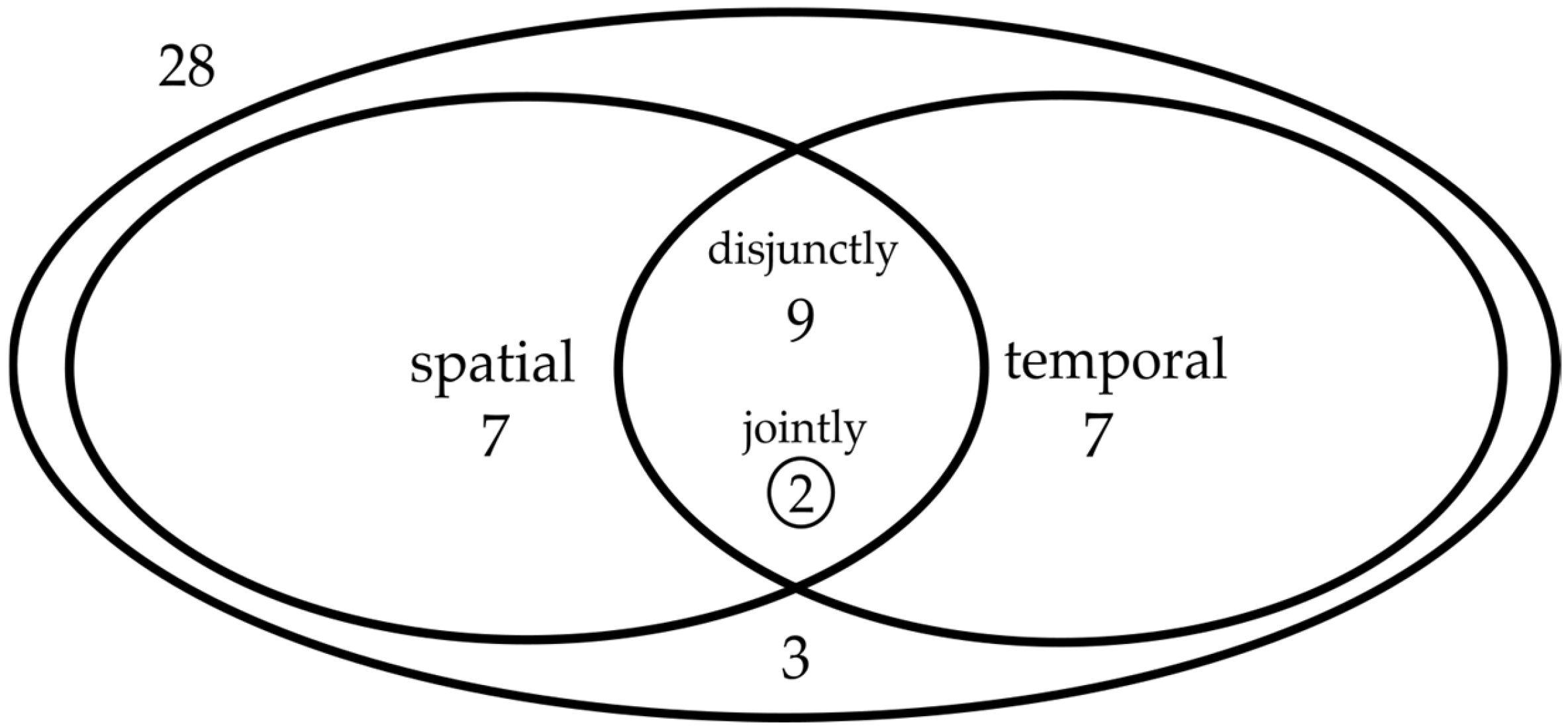
• Temporal Workload Shifting: Analyzed in 18 studies (see also Figure 2), this strategy involves scheduling tasks to times of lower carbon intensity, often coinciding with renewable energy availability.
• Spatial Workload Shifting: Investigated coincidentally also in 18 studies, it focuses on redistributing tasks across geographically diverse data centers, guided by their varying carbon intensities.
• Combined Approaches: A total of 11 of the above studies examined both strategies, suggesting a trend towards integrated approaches for more effective carbon footprint reduction. While in earlier years (i.e., pre-2023), most studies considered either temporal or spatial shifting (13/20 studies, 65%), from the recent literature (i.e., 2024 and 2025), the majority tend to consider both methods (4/5 studies, 80%).
• Beyond Workload Shifting: Five studies proposed different methods for carbon footprint optimization, challenging the sole reliance on workload shifting and indicating a need for diversified strategies.
• Emission Factors: A total of 5 studies used average emission factors, 10 used marginal emission factors, and 10 did not specify their use, highlighting methodological diversity and potential gaps in CI calculation.
• Networking Overhead: Only two studies evaluated the energy requirement due to networking overhead from workload migration, which is generally considered negligible.
• Forecasting: Eight studies employed forecasting techniques, primarily for predicting day-ahead demand or energy prices. However, only two studies detailed their forecasting methods, which raises concerns about methodological transparency and reproducibility.
• Power Mapping: Six studies integrated a mapping of computations to the required power, either by estimation or—for two of them—directly measured, indicating growing interest in accurate energy consumption assessment.
• Embodied emissions: Five studies mentioned embodied emissions but only one detailed its methodology, underscoring the gap of transparent LCA of ICT hardware.
• Optimization Objectives: Of the 28 studies, 10 prioritized minimizing the carbon footprint, with 5 optimizing for an additional objective and 4 considering three objectives simultaneously. Only one study focused exclusively on carbon, highlighting the trend for multi-objective optimization in carbon-aware computing.
• Platform Utilization: Three studies mentioned Kubernetes, one study discussed running their scheduler as a daemon on Linux distributions, while others did not specify a use case.
• Open-Source Availability: Only eight studies have open-sourced their code, raising questions about study reproducibility and comparability within the field.

3.2. Qualitative Analysis

Here, we present two selected topics, which have proven particularly important in the design of our solution presented in Section 4 below.

3.2.1. Embodied Emissions in the Context of Scheduling

Kim et al. [98] utilize performance and energy measurements across diverse application workloads, hourly energy generation data from US power grids, and embodied carbon footprint (CF) modeling tools to quantify the carbon emissions of infrastructure components. Along with being one of the most recent ones in this literature review, it is the most elaborate on topics related to embodied carbon emissions of the infrastructure, mentioning that inclusion of such emission in a holistic optimization framework is still in a “nascent stage”. The authors used both generic LCA methodologies as well as a custom developed Architectural Carbon Tool (ACT) framework [113]. ACT differs from traditional LCA approaches by providing an architecture-specific model for quantifying and optimizing the carbon footprint of computer systems. The advantage of ACT is its specificity, as it focuses on the embodied carbon emissions of hardware manufacturing, considering specific factors like workload characteristics, hardware specifications, and the environmental impacts of semiconductor fabrication processes. To address the lack of data on embodied emissions of hardware, ACT extensively uses data from environmental reports of manufacturers, along with some heuristics over the chip area, indicating a viable option for carbon footprinting in the absence of specialized LCA databases.

3.2.2. Spatio-Temporal Shifting

Most of the studies presented in Table 2 consider either temporal (seven) or spatial (seven) shifting alone. From those that do consider both (nine), the vast majority (seven) only address them separately and not in conjunction. A study that considered both spatial and temporal workload shifting at the same time is that by Bahreini et al. [91]. The authors considered both job-level and load-level optimization and used load forecasts to design a time-slotted system, where for each slot, the information on queued jobs (a tuple of required resources, run time, and deadline) is available. This points out the importance of forecasting to optimally distribute the loads in time. Simultaneously, describing each job with a tuple including required resources seems to be a recurring topic in such studies; however, the inclusion of run time points to the fact that the authors used familiar workloads, which might not be the case in most production environments. The optimization goal of the randomized rounding approximation algorithm is the ratio between CPU utilization and carbon intensity, named “green resource utilization”. Additionally, the authors used a sampling technique to tackle overallocation caused by their algorithm, trading off the schedulability of some pods. Tests showed that the developed algorithm is faster than a traditional high-performance solver for linear programming by several orders of magnitude. The resulting average execution time of the optimization below one second enables online scheduling in cloud environments. The tradeoff of this solution with respect to the traditional solver is the proportion of jobs finishing on time, which is lower by about 10%. Finally, the authors highlighted that after about two thirds of the cluster capacity is reached, using load prediction becomes crucial for adequate job completion times.

3.2.3. Algorithm Development Stages

In

Table 3. Overview of reviewed algorithm development stages, highlighting their strengths and weaknesses.

Maturity Tier	Representative Systems	Salient Strengths	Typical Weaknesses and Open Issues
Industrial deployment/production-grade	CICS [9]; CarbonFlex [96]	Proven fleet-wide or at-scale carbon cuts (≈20–60%) while meeting SLOs Scheduler-agnostic or interoperable designs that fit existing cloud toolchains Continuous learning from historical traces to improve over time	Gains shrink when forecast error rises or deadlines are tight Still depend on accurate job-length prediction and can trigger demand bursts if cluster-wide constraints are mis-tuned
Prototype systems (real clouds/Kubernetes/edge testbeds)	Caspian [92]; Low-Carbon Scheduler [97]; GreenCourier [106]; carbon-aware K8s extender [104]; PlanShare [19]	Work on unmodified public clouds or K8s, easing adoption Exploit geo-diversity, marginal-carbon signals, or locational–marginal–price data Provide empirical evidence of 15–55% CO2 savings with minor QoS impact	Mostly evaluated on hours–weeks traces or small clusters; scalability to cloud-scale remains to be shown Some increase response time or miss deadlines when “sustainability weight” is high Do not yet address embodied-carbon or cross-provider confidentiality hurdles
Advanced research (simulator or trace-driven studies)	FTL meta-algorithm [94]; MinBrown [75]; TTOA/R3DRA [102]; λCO2-shift [101]; GreenScale [98]; EASE [103]; LC-FJSP/CEA-FJSP [110,112]	Show that adaptive algorithm selection, bilevel optimisation, or DRL can add 10–30% extra carbon savings over fixed policies Tackle multi-objective settings (carbon + cost + makespan) and extend to manufacturing and vehicular edge Provide theoretical guarantees or approximation bounds	Results stem from simulation; real-world overheads (migration, forecasting, pricing) not fully captured Carbon benefit fades with high switching cost or short jobs DRL variants struggle with sparse rewards and require large training sets
Conceptual frameworks and holistic analyses	Carbon Explorer [55]; carbond daemon [105]; Sukprasert et al. [107,108]; Let’sWaitAwhile [51]; Carbon Responder [111]	Broaden the problem space: sub-process carbon metering, embodied emissions, demand–response, upper-bound analyses Identify when simple heuristics suffice and where sophisticated methods offer diminishing returns	Often omit algorithmic details or stop at theoretical potential Highlight structural limits: perfect foresight is unrealistic; embodied CO2 can dominate but is rarely acted on

, we present a deeper dive into the review of development stages of the most prominent algorithms, highlighting their respective strengths and weaknesses.

4. Carbon-Aware Spatio-Temporal Workload Shifting: A Novel Algorithm

Allocation problems in computer science are often NP-hard, i.e., no polynomial algorithm can guarantee an optimal solution for all possible instances. These problems, such as bin packing, vehicle routing, and job scheduling, are commonly modeled as Integer Linear Programming (ILP) problems and solved using ILP solvers like CPLEX [114] or through custom heuristic methods when exact solutions are computationally infeasible for large instances. Kubernetes’ scheduling prioritizes flexibility, extensibility, and real-time performance over finding the mathematically optimal solution to the allocation problem, i.e., a solution that is “good enough”. Therefore, in this study, even though we focus on a similar problem setting as [91], we develop straightforward scoring functions that are analogous to the scoring logic in vanilla Kubernetes with additional criteria such as operational and embodied emissions.

In the following subsections, we introduce our approach to allocating carbon footprint (Section 4.1), spatial scoring (Section 4.2), temporal scoring (Section 4.3), and the therefore required load predictions (Section 4.4). Finally, combining the two into spatio-temporal shifting, we provide a heuristic for solving the total carbon minimization problem in Section 4.5.

4.1. Computing a Workload’s Carbon Footprint

As argued earlier, the carbon footprint consists of embodied and operational carbon, which we will discuss now sequentially.

4.1.1. Allocating Embodied Carbon

The embodied carbon of the given node needs to be allocated to each pod that it will be running. LCA standards, such as ISO 14044 [56], propose several options for allocation. The best option is to avoid the allocation altogether, for which two methods exist: (i) dividing the unit process into two or more sub-processes (subdivision), and (ii) expanding the product system to include the additional functions related to the co-products (system expansion). Unfortunately, neither of these methods is suitable to allocating embodied carbon to single tasks in a lifetime of a computational node. Most workloads (including Kubernetes pods, on which focus is placed in this study) are highly integrated, in which the node’s CPU, memory, network, and storage resources are requested and shared dynamically. Such a level of dynamic resource sharing allocation makes it challenging to subdivide the node’s embodied carbon footprint accurately among individual pods. System expansion requires finding or creating equivalent systems that can perform the functions of the co-products (in this case, the services provided by the pods). Given the diverse and specialized functions that pods can perform, from hosting microservices to running batch jobs, identifying or constructing equivalent systems outside of the distributed computing environment is complex and often not feasible.

Since an allocation is not avoidable, we apply the next best option, which is allocation based on the underlying physical relationship between some input of the system (such as energy) and its outputs (such as computation), assuming that the energy consumption is proportional to the consumption of computing resources (such as CPU or RAM). Thus, reserved computing resources that consume electric energy and produce computational output can serve as such physical relationship. In the case of allocating embodied emissions, the input to the system is hardware with associated embodied emissions, and the output stays computation, like in the previous example.

At this stage, an FU (see Section 2.4.2) needs to be defined. Given that Kubernetes pods come with reservation requests for random access memory (RAM) and central processing unit (CPU) cores (one CPU core is equivalent to a vCPU core for cloud providers and a hyperthread on bare-metal Intel processors), we can define an FU as the respective amount of reserved resources for a unit time. Any node can run multiple pods at the same time. We therefore need to allocate the emissions not simply over the pod’s execution time but also over the proportion of the resources reserved for that period, using a product of resources and time. Assuming the time scale in hours and RAM resources measured in GiB (1 GiB = 2³⁰ bytes), this yields an FU for carbon-aware Kubernetes (CAK) defined as:

$${FU}_{CAK}=1 \mathrm{C}\mathrm{P}\mathrm{U} \mathrm{c}\mathrm{o}\mathrm{r}\mathrm{e}\times 1 \mathrm{G}\mathrm{i}\mathrm{B} \mathrm{R}\mathrm{A}\mathrm{M}\times 1 \mathrm{h}\mathrm{o}\mathrm{u}\mathrm{r}$$

(1)

The reservation period of resources is not provided in the specifications of the pod and therefore needs to be estimated based on heuristics.

Table 4. Allocation variables categorized by knowns (left column) and unknows (right column).

Given	To Be Estimated
Pod CPU reservation (${\overline{CPU}}_i$)	Node HW lifetime ($L_j$)
Pod RAM reservation (${\overline{RAM}}_i$) Pod runtime ($U_{ij}$)	Pod power consumption ($P_{ij}$)
Node power supply ACI (${ACI}_{jk}$) Total embodied emissions of node ($C_j^{emb}$) Power curve of node

categorizes the variables necessary for the allocation procedure into knowns and unknowns. The lifetime of node hardware can be taken from the expected lifetime of the respective hardware datasheet, as no better alternative is available. Pod power consumption can be estimated as a function of the utilization rate of the resources with hardware-specific parameters. Finally, pod runtime can be estimated based on historical data related to its time components such as function runtime, data transfer time, and cold start time, as described by [115]. Our current solution, however, will focus on predetermined runtimes for ease of prototyping.

Having defined the FU, we calculate the expected total resources used over the lifetime of a node $j$ (${RU}_j$). This involves multiplying the number of CPU cores $\left(CPU\right)$ and GiB of RAM $\left(RAM\right)$ installed on the node with its total expected operation time $\left(L\right)$ to get the total available resources of the node.

$${RU}_j={CPU}_j\times {RAM}_j\times L_j$$

(2)

Then, we calculate the expected resource usage by the given pod $i \left({\overline{RU}}_{ij}\right)$ as:

$${\overline{RU}}_{ij}={\overline{CPU}}_{ij}\times {\overline{RAM}}_{ij}\times U_{ij}$$

(3)

Now, we can define the proportion of the total resources of the node that was used for executing the given pod as ${\alpha }_{ij}$:

$${\alpha }_{ij}={\displaystyle \frac{{\overline{RU}}_{ij}}{{RU}_j}}$$

(4)

Finally, to get the embodied emissions allocated per pod ($C_{ij}^{emb}$) we multiply the total embodied emissions of the node ($C_j^{emb}$) by this proportion:

$$C_{ij}^{emb}=C_j^{emb}\times {\alpha }_{ij}$$

(5)

4.1.2. Computing Operational Carbon

Expected operational emissions for the given pod are obtained by multiplying the ACI of the electric power used by the node to execute the pod at the given time slot $k$ with the pod’s expected resource reservation time and its power consumption ($P_i$). As with its execution time, we do not have precise data on the pod’s power consumption, but it is conceptually possible to estimate it based on the utilization rate of the node’s hardware by the given pod and the pre-calculated performance curves of the node’s hardware, such as in [116].

$$C_{ijk}^{op}={ACI}_{jk}\times P_{ij}\times U_{ij}$$

(6)

4.2. Spatial Scoring

Spatial scoring is the easiest method of load shifting, since live data on carbon intensity typically suffices for the scheduler to take definitive action. However, unlike temporal scoring (discussed in Section 4.3 below and which takes place within the same node), spatial scoring requires an analysis of embodied emissions for a full picture of the carbon footprint of pod execution. We discussed the procedure of allocating embodied emissions in Section 4.1.1.

To enable the comparison between the nodes, we derive a metric that combines both embodied and operational emissions of a pod on the given node in the form of the “Total Carbo Footprint” or $C_{tot}$ (see Figure 3).

For each node, $C_{tot,ijk}$ comprises an embodied and an operational part according to Equation (7), which combines the results of Equations (5) and (6):

$$C_{tot}=C_{ij}^{emb}+C_{ijk}^{op}$$

(7)

4.3. Temporal Scoring

The scoring procedure for temporal workload shifting requires a more sophisticated approach. Both workload and carbon intensity forecasts now play a crucial role. Since the workload stays on the given node under all circumstances, embodied emissions are no longer relevant as they remain constant.

An important task which has been encapsulated in its own function is the calculation of the so-called “optimal sliding window” (see Figure 4).

We use a sliding window instead of disjunct windows to break down the larger windows in case the workload is executed significantly earlier than the duration of the window expires and thus avoid underutilization during too long a window. Considering the example in Figure 4, we have selected a window length of 2 h for the horizon of 24 h (9 h are shown for legibility). Therefore, if the “now” timestamp corresponds to, e.g., 9 a.m., then the windows available for dispatched workloads are 9 a.m.–11 a.m., 10 a.m.–12 p.m., etc. The resulting hourly resolution is due to the constraint of the hourly CI forecast availability.

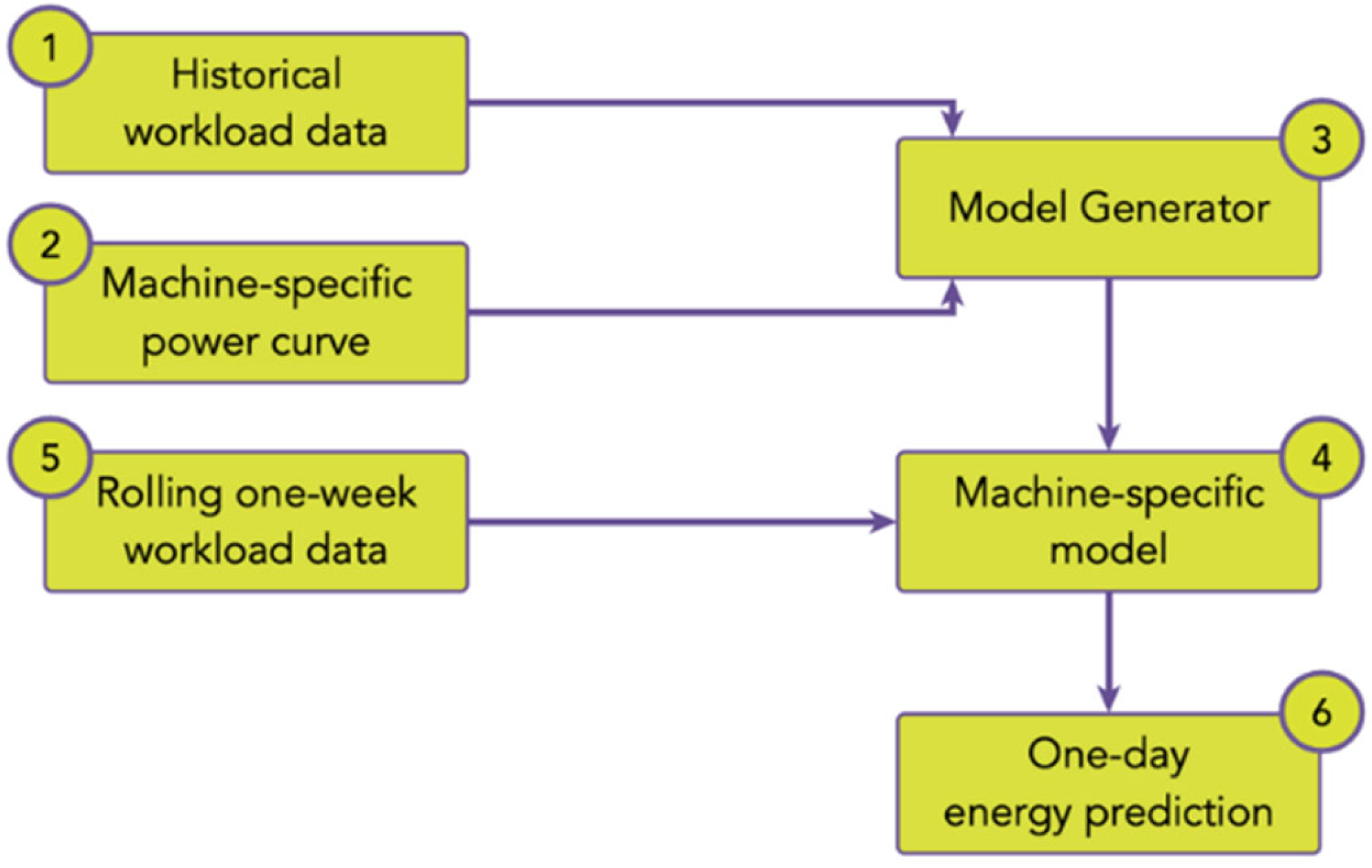
4.4. Workload Prediction Model

The workload prediction model is a crucial component of the carbon-aware scheduler since it allows the scheduler to forecast future demand and optimize task execution accordingly. Temporal shifting is meaningless without such prediction.

As outlined in Section 2.5, the literature on workload prediction is broad and diverse but can be categorized into two main groups: workload-based prediction and power-based prediction. The strength of the former rests in its capacity to predict future resource needs through the analysis of historical workload patterns, whereas the latter concentrates on forecasting immediate power demand by studying power consumption patterns and system performance metrics. Our proposed method integrates both approaches to capitalize on the respective advantages of each.

The model is implemented as a deep learning model, specifically an LSTM network, which is well-suited for time series forecasting. It can capture temporal dependencies and is relatively lightweight to train and deploy. Figure 5 shows the architecture of the model.

Initially, the input data is obtained from a data pipeline that gathers historical workload patterns (1), which include measurements of CPU use and memory consumption. In the current iteration, we employed the Google Cluster Data [117], a dataset of cluster workload traces. In the future, we plan to expand this number of features to disk and network I/O and to automatize the collection of such metrics.

Together with the workload data, a machine-specific power curve (2) is required to explicitly convert the workload figures into realistic power estimates. We employed the SPEC2008 benchmark data [116] in the current iteration. This data is then bundled together, subjected to preprocessing and batching and is finally input into the LSTM network. This initial training data comprises three consecutive weeks of workload data collected at 15 min intervals.

The network is then separately trained (3) on each node to effectively capture the distinct workload patterns that are characteristic to each, yielding (4) a machine-specific model. Once the model is ready, it is capable of reading past workload traces one week at a time (5) and forecasting workload patterns over the upcoming 24 h (6).

The model’s accuracy greatly varies on the data it is trained on, and thus, on the workload patterns of the node it is deployed on. From the Google Cluster Data, we selected two machines that exhibit distinct workload patterns. The first machine is characterized by very cyclic workload patterns, where night hours are almost idle and day hours exhibit a very high and varying CPU and memory usage. The second machine, on the other hand, has a more stable workload pattern, with a lower CPU and memory usage that does not vary much over time. We repeated the experiment several times, each time selecting 21 consecutive days of data for training and 21 additional consecutive and unseen days for testing (strictly separated and picked from a later period). The model then attempts to predict the workload for the next hour (both CPU and memory as intervals between 0 and 1) with an MSE that is, on average, between 0.01 (for the second machine) and 0.05 (for the first machine); however, we observed some corner-case outliers with an MSE of up to 3.5, which was likely due to the variability in the workload patterns.

This architecture is deployed as a service on every node, where it consistently receives real-time workload data and refreshes its predictions. In its current iteration, the figures the model produces are converted to a power score using the machine-specific power curve. This score is then used as an input for the temporal scoring method.

4.5. Spatio-Temporal Shifting Algorithm

The algorithm for carbon-aware spatio-temporal shifting of Kubernetes pods developed in the scope of this study (see Algorithm 1) is based on concepts introduced in Section 4.2 and Section 4.3. It aims to minimize carbon emissions by efficiently scheduling pods across geographically distributed nodes and time slots.

To make the proposed algorithm work effectively, several key assumptions need to be made. These assumptions provide the foundation for the algorithm’s logic and operational parameters:

• Access to CI data (good data available and deployed).
• Pod resource requirements specific to the node (the trickiest assumption; heuristics need to be developed).
• Data on expected lifetimes of hardware (existing but scattered).
• Availability of power curves (good data for DC servers, incipient for edge devices).
• Availability of embodied emissions data (existing, but typically only for categories of devices, not individual products).

The algorithm begins with an initialization phase where key structures are set up. An empty schedule $S$ is initialized, and resource availability matrices $R_{jk}$ for all nodes $j$ and time slots $k$ are established. The embodied emissions rate $C_j^{emb}$ for each node $j$ is calculated once, as it does not change over time.

The main loop of the algorithm checks for new pod arrivals and updates the carbon intensity and utilization data for the next 24 h every hour based on new forecasts. This ensures that scheduling decisions are always based on the latest available data. When new pods arrive, they are added to the priority queue $Q$ based on their deadlines. This prioritization ensures that more urgent pods are considered first, improving the likelihood that critical deadlines are met.

At each hourly update or when new pods arrive, the algorithm re-evaluates the scheduling of pods. For each pod $i$ in the priority queue $Q$, the algorithm initializes the minimum emissions $C^{\ast }$ to infinity and sets the value for the optimal node $j^{\ast }$ and optimal time slot $k^{\ast }$ to −1, indicating that no optimal slot has been found yet. The algorithm then iterates over each possible time slot $k$ and each node $j$ to find the best scheduling option. First, it checks if the end of the time slot ${End}_k$ is within the pod’s deadline ${Deadline}_i$. This ensures that the pod will complete its execution before its specified deadline.

Next, the algorithm verifies that node $j$ has sufficient CPU and RAM to accommodate pod $i$. This is essential to ensure that the node can handle the resource requirements of the pod without causing performance issues or failures. The check involves comparing the pod’s requirements to the node’s available resources.

The algorithm then examines the utilization of the node. It identifies the set $S_{jk}$ of pods already scheduled on node $j$ at time slot $k$ and checks whether the total duration of these pods, plus the duration of the current pod $i$, does not exceed the available capacity of the node. This check ensures that the node is not overloaded and that all scheduled pods can be executed within the time slot.

For each potential scheduling option, the algorithm computes the operational emissions for scheduling pod $i$ on node $j$ at time slot $k$. The operational emissions $C_{ijk}^{op}$ are calculated based on the average carbon intensity, the duration of the pod, and its power consumption (from the proportion of the resources utilized by the pod to total utilization). Additionally, the total power consumption on node $j$ after adding pod $i$ is computed. This allows the algorithm to determine the proportion of operational missions attributable to the pod, which is essential for accurately calculating the total emissions.

The total emissions $C_{tot}$ are then computed by adding the operational emissions to the proportion of the embodied emissions based on the pod’s power consumption relative to the node’s total power consumption. This proportional allocation ensures that the embodied emissions are fairly distributed among all pods running on the node at the same time.

If the calculated total emissions $C_{tot}$ are less than the current minimum emissions $C^{\ast }$, the algorithm updates $C^{\ast }$, $j^{\ast }$, and $k^{\ast }$. This step ensures that the algorithm always seeks to minimize emissions.

After evaluating all time slots and nodes for the current pod $i$, the algorithm decides whether to schedule the pod. If a feasible node and time slot are found, the pod is scheduled on $j^{\ast }$ at $k^{\ast }$. The schedule $S$ is updated accordingly, and the pod is removed from the priority queue $Q$. If no feasible option is found, the pod is reinserted into the priority queue with updated priority, ensuring that it will be reconsidered in future iterations.

The algorithm then waits for the next hourly update or the arrival of new pods before re-evaluating the scheduling. This continuous loop ensures that the scheduling decisions are dynamically adjusted based on the latest data and conditions.

Algorithm 1. Spatio-temporal shifting (ijk represent pod, node, and time slot, respectively, overline denotes pod-related resources, and hat is used to signify predicted variables).

Input: Priority queue Q of pods; set of nodes N; set of time slots T; resource requirements and deadlines of pods; predicted average carbon intensities (ACI) and utilization of nodes.

Result: Feasible schedule S of pods on nodes and time slots that minimizes total carbon emissions.

Initialize empty schedule S

Initialize resource availability Rjk for all nodes j ∈ N and time slots k ∈ T

Calculate embodied emissions rate $c_j^{emb}$ for each node j as $c_j^{emb}={\displaystyle \frac{c_j^{emb}}{L_j}}$

If new pods arrived then

Add new pods to the priority queue Q based on their deadlines

End If

If hourly update or new pods arrive then

For each pod i ∈ Q do

Set C* ← ∞; j* ← −1; k* ← −1

For each time slot k ∈ T do

If Endk ≤ Deadlinei then

For each node j ∈ N do

If CPU and RAM constraints are satisfied then

If utilization constraint is satisfied then

$C_{ijk}^{op}={\widehat{ACI}}_{jk}\times U_i\times P_i$

$P_{tot}={\displaystyle {\sum }_{m\in S_{jk}}{P}_m}+P_i$

$C_{tot}=C_{ijk}^{op}+\left(c_j^{emb}\times U_i\times {\displaystyle \frac{P_i}{P_{tot}}}\right)$

If Ctot < C* then

C* ← Ctot; j* ← j; k* ← k

End If

End If

End If

End For

End If

End For

If j* ≠ −1 and k* ≠ −1 then

Schedule pod i on node j* at time slot k*

Update schedule S

Remove pod i from Q

End If

End For

End If

5. Discussion and Limitations

As stated from the outset, the main aims of this paper were to review existing carbon-aware scheduling techniques and, building on the insights from this review, to suggest a novel, integrated spatio-temporal shifting algorithm, which takes into account not only operational emissions but also the carbon embodied during device production and deploys a workload forecast paradigm. These numerous conceptual contributions notwithstanding, the main limitation of our solution at this stage is the not yet fully developed implementation.

As presented in Section 4.4, the workload predictor has already been implemented and is publicly available. The rest of the algorithm is under development and will be presented in a subsequent publication. We have a clear roadmap for implementation and testing, as presented in Section 6 below.

5.1. Algorithm

Understanding the implications of the proposed carbon-aware scheduling algorithm is crucial for assessing its feasibility and effectiveness in real-world scenarios. This subsection discusses the computational overhead, complexity, Quality of Service (QoS) effects, and the carbon footprint of the algorithm to provide a comprehensive evaluation.

Overhead. The algorithm induces computing overhead as it iterates over each pod in the priority queue, evaluating all possible time slots for each participating node. Memory overhead stems from storing the priority queue and tracking resource availability for all nodes and time slots, in addition to maintaining intermediate results like the set of already scheduled pods on each node and time slot. Rather negligible I/O overhead results from retrieving periodic updates for carbon intensity and utilization forecasts.

Complexity. Finding the globally optimal carbon-aware spatio-temporal schedule has been shown to belong to the class of bin-packing problems and is thus NP-hard [52,91]. By contrast, and to avoid NP-hardness, our algorithm does not aim to find the perfect schedule for all pods but just for that at the front of the queue. The gain is a polynomial algorithm, and the price is a globally non-optimal solution (but still one that optimizes carbon). Its complexity, while polynomial, is nevertheless considerable, being directly proportional to $P\times T\times N\times M$, where $P$ is the number of pods, $T$ is the number of time slots, $N$ is the number of nodes, and $M$ is the maximum number of pods that can be scheduled on a node in a time slot.

Quality of Service. The algorithm has a twofold impact on the Quality of Service. On the positive side, it enhances resource utilization by ensuring that nodes are not overburdened, thus maintaining optimal performance and reducing resource contention. The priority queue management allows urgent pods to be scheduled first, improving response times for high-priority tasks. Moreover, by considering carbon intensity in scheduling decisions, it contributes to a greener infrastructure. However, the complexity of the scheduling process and frequent re-evaluation can introduce delays in pod execution, especially under heavy workloads. Additionally, the increased CPU usage and longer scheduling times due to the algorithm’s complexity might negatively impact overall system performance.

Carbon Footprint. The carbon footprint of the algorithm includes both direct and indirect effects. Directly, the algorithm’s execution consumes computational resources such as CPU and memory, contributing to the operational carbon footprint. The need for periodic updates and data processing also adds to the carbon footprint through associated I/O and computation. Indirectly, due to its main aim, the algorithm helps reduce the overall carbon footprint by optimizing pod placement to minimize carbon emissions. Efficiently distributed workloads across nodes can lead to better utilization of energy-efficient nodes and selecting time slots with lower carbon intensity. This balance between the algorithm’s direct resource consumption and its contribution to overall carbon efficiency is a key consideration in evaluating its environmental impact.

Implementation. The implementation of the aforementioned algorithm is bound to the development of a computing continuum architecture to which our research contributes [118], and therefore, parts of its implementation are still pending. This work is currently being validated within the context of the research project “FLUIDOS” [13] under the EU’s funding program “Horizon 2020”.

5.2. Environmental Evaluation

To achieve a more holistic understanding of the environmental footprint of computation, it is essential to consider indicators beyond just energy consumption and carbon emissions. The following paragraphs explore additional environmental impacts and the limitations of life cycle assessment (LCA) in this context.

Environmental Impact Beyond Energy and Carbon. An expansion of environmental scope to include indicators other than global warming potential would be required for a more comprehensive picture of the environmental footprint of computation. Given that ICT hardware relies on various abiotic resources, including rare earth elements and metals, whose extraction and processing can lead to significant environmental degradation, the “Abiotic Resource Depletion” indicator is among the first candidates to be considered in scheduling of computational tasks. As this impact occurs overwhelmingly during production, accounting for the embodied resource use would here be mandatory; this is another argument for the validity of our production-including approach. The water consumption of data centers is a growing concern, in particular related to AI training and inference. Training one large language model is directly responsible for hundreds of thousands [119] to millions [120] of liters of freshwater. Given the expected AI growth, accounting for the indirect water usage during electricity production and including inference as well might lead to an AI-generated water withdrawal several orders of magnitude higher over the next years [119]. “Water Footprint” is thus arguably the most important candidate for future scrutiny.

LCA Limitations. While our carbon-aware scheduling algorithm is designed to optimize resource allocation and minimize carbon emissions, it has several weaknesses when relying on LCA data for embodied emissions. One significant limitation is the complexity and time required to conduct a comprehensive LCA, which involves gathering extensive data across the entire lifecycle of computing hardware—from raw material extraction to disposal. This process can be resource-intensive and may not always provide timely insights for fast-paced technological environments. Additionally, the accuracy of LCA results can be compromised by the quality and availability of data, leading to potential gaps and uncertainties in the assessment. For our algorithm, this means that inaccuracies or inconsistencies in the embodied emissions data can bias scheduling decisions, potentially undermining the goal of minimizing total carbon emissions. Another challenge is the difficulty in standardizing LCA methodologies, as different studies may use varied assumptions and system boundaries, making comparisons and integrations across datasets problematic.

6. Conclusions and Further Work

This paper contributes to the field of carbon-aware computing in two ways: It provides a comprehensive literature review and introduces a novel spatio-temporal shifting algorithm that addresses gaps identified in the existing literature.

In our literature review, we revealed that two main methods are deployed: temporal workload shifting involves scheduling tasks during times of lower carbon intensity, often coinciding with renewable energy availability, while spatial workload shifting redistributes tasks across geographically diverse data centers based on carbon intensities. An emerging trend is the integration of both temporal and spatial strategies for more effective carbon footprint reduction; however, the two are usually considered alternatively and not jointly.

While most previous studies predominantly focus on either spatial or temporal shifting, our work integrates both. The main idea of our algorithm is simple but effective. To predict the availability of computation resources necessary for shifts into the future, we presented an ML-based algorithm combining workload-based prediction and power-based prediction. By incorporating device production emissions into our model, we address an often-overlooked aspect of carbon footprinting, thereby offering a more comprehensive understanding of environmental impacts. Given the continuing decarbonization of operational electricity driven by various IT companies, the relative importance of the embodied impact is bound to grow.

Future research should focus on refining our algorithm’s forecasting capabilities to enhance its predictive accuracy and efficiency. Investigating the scalability of the algorithm across diverse computing environments and its applicability to edge computing scenarios will also be crucial. We aim to develop more sophisticated models for accounting for the embodied emissions of computing hardware, further improving the environmental sustainability of computing operations. Here, a dynamic categorization strategy for hardware may yield additional benefits if proven feasible in the experimental phase. A better method needs to be devised, in particular for the prediction of a pod’s runtime. The overhead of the algorithm requires a more thorough investigation; next to the complexity it inherently brings, there might be thresholds below which this overhead might not be energetically justified. Finally, the developed framework will be tested on real infrastructure consisting of multiple geographically distributed nodes, providing a reference for transferability of the analytic results. To achieve this, an emulation environment is planned to be developed, first based on KWOK [121]. It will be used to explore the relevant testing scenarios. The fully developed algorithm framework will then be deployed on real infrastructure nodes to quantify carbon savings and latency penalty tradeoffs.

References

1. Andrae, A.S.G.; Edler, T. On Global Electricity Usage of Communication Technology: Trends to 2030. Challenges 2015, 6, 117–157. [Google Scholar] [CrossRef]
2. Malmodin, J.; Lundén, D. The Energy and Carbon Footprint of the Global ICT and E&M Sectors 2010–2015. Sustainability 2018, 10, 3027. [Google Scholar] [CrossRef]
3. Basmadjian, R. Flexibility-Based Energy and Demand Management in Data Centers: A Case Study for Cloud Computing. Energies 2019, 12, 3301. [Google Scholar] [CrossRef]
4. Marcel, A.; Cristian, P.; Eugen, P.; Claudia, P.; Cioara, T.; Anghel, I.; Ioan, S. Thermal aware workload consolidation in cloud data centers. In Proceedings of the 2016 IEEE 12th International Conference on Intelligent Computer Communication and Processing (ICCP), Cluj-Napoca, Romania, 8–10 September 2016; IEEE: New York, NY, USA, 2016; pp. 377–384. [Google Scholar] [CrossRef]
5. Rong, H.; Zhang, H.; Xiao, S.; Li, C.; Hu, C. Optimizing energy consumption for data centers. Renew. Sustain. Energy Rev. 2016, 58, 674–691. [Google Scholar] [CrossRef]
6. Sotos, M.; Didden, M.; Kovac, A.; Ryor, J.; Stevens, A.; Cummis, C. GHG Protocol Scope 2 Guidance; Greenhouse Gas Protocol: Washington, DC, USA, 2015. [Google Scholar]
7. Holzapfel, P.; Bach, V.; Finkbeiner, M. Electricity accounting in life cycle assessment: The challenge of double counting. Int. J. Life Cycle Assess 2023, 28, 771–787. [Google Scholar] [CrossRef]
8. Biswas, D.; Jahan, S.; Saha, S.; Samsuddoha, M. A succinct state-of-the-art survey on green cloud computing: Challenges, strategies, and future directions. Sustain. Comput. Inform. Syst. 2024, 44, 101036. [Google Scholar] [CrossRef]
9. Radovanovic, A.; Koningstein, R.; Schneider, I.; Chen, B.; Duarte, A.; Roy, B.; Xiao, D.; Haridasan, M.; Hung, P.; Care, N.; et al. Carbon-Aware Computing for Datacenters. IEEE Trans. Power Syst. 2021, 38, 1270–1280. Available online: http://arxiv.org/abs/2106.11750 (accessed on 20 July 2023).
10. Kubernetes Documentation. Available online: https://kubernetes.io/docs/home/ (accessed on 15 May 2024).
11. Hischier, R.; Coroama, V.C.; Schien, D.; Achachlouei, M.A. Grey Energy and Environmental Impacts of ICT Hardware. In ICT Innovations for Sustainability; Hilty, L.M., Aebischer, B., Eds.; Advances in Intelligent Systems and Computing; Springer International Publishing: Cham, Switzerland, 2015; Volume 310, pp. 171–189. [Google Scholar] [CrossRef]
12. Fluidos-Energy-Predictor. 2024. Available online: https://github.com/fluidos-project/fluidos-energy-predictor (accessed on 10 May 2024).
13. Fluidos, Creating a Fluid, Dynamic, Scalable, and Trustable Computing Continuum. Available online: https://www.fluidos.eu/ (accessed on 24 July 2024).
14. IEA. Electricity 2024: Analysis and Forecast to 2026; IEA: Paris, France, 2024. [Google Scholar]
15. OpenAI, ChatGPT. 2024. Available online: https://openai.com/chatgpt (accessed on 18 January 2024).
16. Google, Gemini-Chat to Supercharge Your Ideas. 2024. Available online: https://gemini.google.com (accessed on 29 May 2024).
17. Meta, Llama 3. 2024. Available online: https://llama.meta.com/llama3/ (accessed on 29 May 2024).
18. Wired, The Generative AI Race Has a Dirty Secret. Available online: https://www.wired.com/story/the-generative-ai-search-race-has-a-dirty-secret/ (accessed on 18 January 2024).
19. Lin, L.; Chien, A. Adapting Datacenter Capacity for Greener Datacenters and Grid. In Proceedings of the 14th ACM International Conference on Future Energy Systems, Orlando, FL, USA, 16–23 June 2023; pp. 200–213. [Google Scholar] [CrossRef]
20. Moore, G.E. Cramming more components onto integrated circuits. Electronics 1965, 38, 114–117. [Google Scholar] [CrossRef]
21. Hintemann, R.; Hinterholzer, S. Energy consumption of data centers worldwide. ICT4S. 2019. Available online: https://ceur-ws.org/Vol-2382/ICT4S2019_paper_16.pdf (accessed on 7 July 2025).
22. Malmodin, J.; Lövehagen, N.; Bergmark, P.; Lundén, D. ICT sector electricity consumption and greenhouse gas emissions—2020 outcome. Telecommun. Policy 2024, 48, 102701. [Google Scholar] [CrossRef]
23. Galantino, S.; Risso, F.; Coroamă, V.C.; Manzalini, A. Assessing the Potential Energy Savings of a Fluidified Infrastructure. Computer 2023, 56, 26–34. [Google Scholar] [CrossRef]
24. National Grid Group. What Is Carbon Intensity? Available online: https://web.archive.org/web/20240414132036/https://www.nationalgrid.com/stories/energy-explained/what-is-carbon-intensity (accessed on 9 October 2023).
25. Listgarten, S. When to Use Marginal Emissions (and When Not To). Available online: https://web.archive.org/web/*/https://www.paloaltoonline.com/blogs/p/2019/09/29/marginal-emissions-what-they-are-and-when-to-use-them (accessed on 9 October 2023).
26. Electricity Maps. Marginal vs Average: Which One to Use for Real-Time Decisions? Available online: https://www.electricitymaps.com/blog/marginal-vs-average-real-time-decision-making (accessed on 19 April 2024).
27. WattTime. Available online: https://www.watttime.org/ (accessed on 9 October 2023).
28. Electricity Maps. Live 24/7 CO2 Emissions of Electricity Consumption. Available online: http://electricitymap.tmrow.co (accessed on 29 May 2024).
29. NESO. Carbon Intensity. Available online: https://carbonintensity.org.uk/ (accessed on 9 October 2023).
30. EIA. Hourly Electric Grid Monitor. Available online: https://www.eia.gov/electricity/gridmonitor/index.php (accessed on 9 October 2023).
31. ENTSO-E. ENTSO-E Transparency Platform. Available online: https://transparency.entsoe.eu/ (accessed on 9 October 2023).
32. Kubernetes Carbon Intensity Exporter. (27 September 2023). Go. Microsoft Azure. Available online: https://github.com/Azure/kubernetes-carbon-intensity-exporter (accessed on 5 October 2023).
33. Carbon Aware SDK. (29 September 2023). C#. Green Software Foundation. Available online: https://github.com/Green-Software-Foundation/carbon-aware-sdk (accessed on 5 October 2023).
34. KEDA. Available online: https://keda.sh/docs/2.13/concepts/ (accessed on 17 February 2024).
35. Gao, X.; Liu, R.; Kaushik, A. Hierarchical Multi-Agent Optimization for Resource Allocation in Cloud Computing. IEEE Trans. Parallel Distrib. Syst. 2021, 32, 692–707. [Google Scholar] [CrossRef]
36. Elhady, G.F.; Tawfeek, M.A. A comparative study into swarm intelligence algorithms for dynamic tasks scheduling in cloud computing. In Proceedings of the 2015 IEEE Seventh International Conference on Intelligent Computing and Information Systems (ICICIS), Cairo, Egypt, 12–14 December 2015; IEEE: New York, NY, USA, 2015; pp. 362–369. [Google Scholar] [CrossRef]
37. Saxena, R.; Afrin, N. Comparison of Scheduling Algorithms in Cloud Computing. In Proceedings of the National Conference on Computer Security, Image Processing, Graphics, Mobility and Analytics, Telangana, India, 17–18 December 2016; pp. 37–40. [Google Scholar] [CrossRef]
38. Pacini, E.; Mateos, C.; Garino, C.G. Balancing throughput and response time in online scientific Clouds via Ant Colony Optimization (SP2013/2013/00006). Adv. Eng. Softw. 2015, 84, 31–47. [Google Scholar] [CrossRef]
39. Singh, P.; Dutta, M.; Aggarwal, N. Bi-objective HWDO Algorithm for Optimizing Makespan and Reliability of Workflow Scheduling in Cloud Systems. In Proceedings of the 2017 14th IEEE India Council International Conference (INDICON), Roorkee, India, 15–17 December 2017; IEEE: New York, NY, USA, 2017; pp. 1–9. [Google Scholar] [CrossRef]
40. Kaur, T.; Pahwa, S. An Upgraded Algorithm of Resource Scheduling using PSO and SA in Cloud Computing. Int. J. Comput. Appl. 2013, 74, 28–32. [Google Scholar] [CrossRef]
41. Wu, W.; Lin, W.; Peng, Z. An intelligent power consumption model for virtual machines under CPU-intensive workload in cloud environment. Soft Comput. 2017, 21, 5755–5764. [Google Scholar] [CrossRef]
42. Beegom, A.S.A.; Rajasree, M.S. Integer-PSO: A discrete PSO algorithm for task scheduling in cloud computing systems. Evol. Intell. 2019, 12, 227–239. [Google Scholar] [CrossRef]
43. Dubey, H.M.; Pandit, M.; Srivastava, L.; Panigrahi, B.K. (Eds.) Artificial Intelligence and Sustainable Computing: Proceedings of ICSISCET 2020; Springer Nature: Singapore, 2022. [Google Scholar] [CrossRef]
44. Zuo, L.; Shu, L.; Dong, S.; Zhu, C.; Hara, T. A Multi-Objective Optimization Scheduling Method Based on the Ant Colony Algorithm in Cloud Computing. IEEE Access 2015, 3, 2687–2699. [Google Scholar] [CrossRef]
45. Fard, H.M.; Prodan, R.; Barrionuevo, J.J.D.; Fahringer, T. A Multi-objective Approach for Workflow Scheduling in Heterogeneous Environments. In Proceedings of the 2012 12th IEEE/ACM International Symposium on Cluster, Cloud and Grid Computing (CCGRID 2012), Ottawa, ON, Canada, 13–16 May 2012; IEEE: New York, NY, USA, 2012; pp. 300–309. [Google Scholar] [CrossRef]
46. Lu, X.; Tang, S. Synchronous Dislocation Scheduling Quantum Algorithm Optimization in Virtual Private Cloud Computing Environment. In Proceedings of the 2022 6th International Conference on Intelligent Computing and Control Systems (ICICCS), Madurai, India, 25–27 May 2022; pp. 596–599. [Google Scholar] [CrossRef]
47. Zandvakili, A.; Mansouri, N.; Javidi, M.M. A Fuzzy based Pathfinder Optimization Technique for Performance-Effective Task Scheduling in Cloud. AUT J. Model. Simul. 2021, 53, 197–216. [Google Scholar] [CrossRef]
48. Vinothkumar, K.; Maruthanayagam, D. Comprehensive Study On EDGE-Cloud Collaborative Computing for Optimal Task Scheduling. Int. J. Sci. Res. Comput. Sci. Eng. Inf. Technol. 2022, 8, 75–90. [Google Scholar] [CrossRef]
49. Piroozfard, H.; Wong, K.Y.; Wong, W.P. Minimizing total carbon footprint and total late work criterion in flexible job shop scheduling by using an improved multi-objective genetic algorithm. Resour. Conserv. Recycl. 2018, 128, 267–283. [Google Scholar] [CrossRef]
50. Chen, C.; He, B.; Tang, X. Green-aware workload scheduling in geographically distributed data centers. In Proceedings of the 2012 IEEE 4th International Conference on Cloud Computing Technology and Science (CloudCom), Taipei, Taiwan, 3–6 December 2012; IEEE: New York, NY, USA, 2012; pp. 82–89. [Google Scholar] [CrossRef]
51. Wiesner, P.; Behnke, I.; Scheinert, D.; Gontarska, K.; Thamsen, L. Let’s Wait Awhile: How Temporal Workload Shifting Can Reduce Carbon Emissions in the Cloud. In Proceedings of the 22nd International Middleware Conference, Quebec City, QC, Canada, 6–10 December 2021; pp. 260–272. [Google Scholar] [CrossRef]
52. Khodayarseresht, E.; Shameli-Sendi, A.; Fournier, Q.; Dagenais, M. Energy and carbon-aware initial VM placement in geographically distributed cloud data centers. Sustain. Comput. Inform. Syst. 2023, 39, 100888. [Google Scholar] [CrossRef]
53. Rawas, S.; Zekri, A.; El-Zaart, A. LECC: Location, energy, carbon and cost-aware VM placement model in geo-distributed DCs. Sustain. Comput. Inform. Syst. 2021, 33, 100649. [Google Scholar] [CrossRef]
54. Yang, T.; Jiang, H.; Hou, Y.; Geng, Y. Carbon Management of Multi-Datacenter Based on Spatio-Temporal Task Migration. IEEE Trans. Cloud Comput. 2023, 11, 1078–1090. [Google Scholar] [CrossRef]
55. Acun, B.; Lee, B.; Kazhamiaka, F.; Maeng, K.; Gupta, U.; Chakkaravarthy, M.; Brooks, D.; Wu, C.-J. Carbon Explorer: A Holistic Approach for Designing Carbon Aware Datacenters. In Proceedings of the 28th ACM International Conference on Architectural Support for Programming Languages and Operating Systems, Vancouver, BC, Canada, 25–29 March 2023; Volume 2, pp. 118–132. [Google Scholar] [CrossRef]
56. DIN EN ISO 14044-2006; Environmental Management—Life Cycle Assessment—Requirements and Guidelines. ISO: Geneva, Switzerland, 2006.
57. Finkbeiner, M. Carbon footprinting—Opportunities and threats. Int. J. Life Cycle Assess. 2009, 14, 91–94. [Google Scholar] [CrossRef]
58. Gröger, J.; Liu, R.; Stobbe, L.; Druschke, J.; Richter, N. Green Cloud Computing: Lebenszyklusbasierte Datenerhebung zu Umweltwirkungen des Cloud Computing; Federal Environment Agency: Berlin, Germany, 2021.
59. Wäger, P.A.; Hischier, R.; Widmer, R. The Material Basis of ICT. In ICT Innovations for Sustainability; Hilty, L.M., Aebischer, B., Eds.; Advances in Intelligent Systems and Computing; Springer International Publishing: Cham, Switzerland, 2015; Volume 310, pp. 209–221. [Google Scholar] [CrossRef]
60. DIN EN ISO 14040; Environmental Management—Life Cycle Assessment—Principles and Framework. ISO: Geneva, Switzerland, 2006. [CrossRef]
61. Weidema, B.; Wenzel, H.; Petersen, C.; Hansen, K. The Product, Functional Unit and Reference Flows in LCA; Danish Environmental Protection Agency: Odense, Denmark, 2004.
62. Deng, L.; Williams, E.D. Functionality Versus “Typical Product” Measures of Technological Progress: A Case Study of Semiconductor Manufacturing. J. Ind. Ecol. 2011, 15, 108–121. [Google Scholar] [CrossRef]
63. Mars, C.; Nafe, C.; Linnell, J. The Electronics Recycling Landscape Report; The Sustainable Consortium: Tempe, AZ, USA, 2016. [Google Scholar]
64. Whitehead, B.; Andrews, D.; Shah, A. Maidment Assessing the environmental impact of data centres part 2: Building environmental assessment methods and life cycle assessment. Build. Environ. 2015, 93, 395–405. [Google Scholar] [CrossRef]
65. Makov, T.; Fishman, T.; Chertow, M.R.; Blass, V. What Affects the Secondhand Value of Smartphones: Evidence from eBay. J. Ind. Ecol. 2019, 23, 549–559. [Google Scholar] [CrossRef]
66. Grobe, K. Energy Efficiency Limits to ICT Lifetime. In Proceedings of the 23th ITG-Symposium, Berlin, Germany, 18–19 May 2022. [Google Scholar]
67. Masanet, E.; Shehabi, A.; Koomey, J. Characteristics of low-carbon data centres. Nat. Clim. Change 2013, 3, 627–630. [Google Scholar] [CrossRef]
68. Boavizta/Environmental-Footprint-Data. (20 June 2025). Python. Boavizta. Available online: https://github.com/Boavizta/environmental-footprint-data (accessed on 4 July 2025).
69. Dayarathna, M.; Wen, Y.; Fan, R. Data Center Energy Consumption Modeling: A Survey. IEEE Commun. Surv. Tutor. 2016, 18, 732–794. [Google Scholar] [CrossRef]
70. Jin, C.; Bai, X.; Yang, C.; Mao, W.; Xu, X. A review of power consumption models of servers in data centers. Appl. Energy 2020, 265, 114806. [Google Scholar] [CrossRef]
71. Mosavi, A.; Bahmani, A. Energy Consumption Prediction Using Machine Learning; A Review. Engineering 2019. preprints. [Google Scholar] [CrossRef]
72. Depasquale, E.-V.; Davoli, F.; Rajput, H. Dynamics of Research into Modeling the Power Consumption of Virtual Entities Used in the Telco Cloud. Sensors 2022, 23, 255. [Google Scholar] [CrossRef]
73. Bohra, A.E.H.; Chaudhary, V. VMeter: Power modelling for virtualized clouds. In Proceedings of the 2010 IEEE International Symposium on Parallel & Distributed Processing, Workshops and Phd Forum (IPDPSW), Atlanta, GA, USA, 19–23 April 2010; IEEE: New York, NY, USA, 2010; pp. 1–8. [Google Scholar] [CrossRef]
74. Li, Y.; Wang, Y.; Yin, B.; Guan, L. An Online Power Metering Model for Cloud Environment. In Proceedings of the 2012 IEEE 11th International Symposium on Network Computing and Applications, Cambridge, MA, USA, 23–25 August 2012; pp. 175–180. [Google Scholar] [CrossRef]
75. Chen, F.; Schneider, J.-G.; Yang, Y.; Grundy, J.; He, Q. An energy consumption model and analysis tool for Cloud computing environments. In Proceedings of the 2012 First International Workshop on Green and Sustainable Software (GREENS), Zurich, Switzerland, 3 June 2012; IEEE: New York, NY, USA, 2012; pp. 45–50. [Google Scholar] [CrossRef]
76. Krishnan, B.; Amur, H.; Gavrilovska, A.; Schwan, K. VM power metering: Feasibility and challenges. ACM Sigmetrics Perform. Eval. Rev. 2011, 38, 56–60. [Google Scholar] [CrossRef]
77. Xiao, P.; Hu, Z.; Liu, D.; Yan, G.; Qu, X. Virtual machine power measuring technique with bounded error in cloud environments. J. Netw. Comput. Appl. 2013, 36, 818–828. [Google Scholar] [CrossRef]
78. Da Costa, G.; Hlavacs, H. Methodology of measurement for energy consumption of applications. In Proceedings of the 2010 11th IEEE/ACM International Conference on Grid Computing, Brussels, Belgium, 25–28 October 2010; IEEE: New York, NY, USA, 2010; pp. 290–297. [Google Scholar] [CrossRef]
79. Kansal, A.; Zhao, F.; Liu, J.; Kothari, N.; Bhattacharya, A.A. Virtual machine power metering and provisioning. In Proceedings of the 1st ACM Symposium on Cloud Computing, Indianapolis, IN, USA, 10–11 June 2010; ACM: New York, NY, USA, 2010; pp. 39–50. [Google Scholar] [CrossRef]
80. Chen, Q.; Grosso, P.; van der Veldt, K.; de Laat, C.; Hofman, R.; Bal, H. Profiling Energy Consumption of VMs for Green Cloud Computing. In Proceedings of the 2011 IEEE Ninth International Conference on Dependable, Autonomic and Secure Computing, Sydney, Australia, 10–14 December 2011; IEEE: New York, NY, USA, 2011; pp. 768–775. [Google Scholar] [CrossRef]
81. Dhiman, G.; Mihic, K.; Rosing, T. A system for online power prediction in virtualized environments using Gaussian mixture models. In Proceedings of the 47th Design Automation Conference, Anaheim, CA, USA, 13–18 June 2010; ACM: New York, NY, USA, 2010; pp. 807–812. [Google Scholar] [CrossRef]
82. Yang, H.; Zhao, Q.; Luan, Z.; Qian, D. iMeter: An integrated VM power model based on performance profiling. Futur. Gener. Comput. Syst. 2013, 36, 267–286. [Google Scholar] [CrossRef]
83. Song, S.; Su, C.; Rountree, B.; Cameron, K.W. A Simplified and Accurate Model of Power-Performance Efficiency on Emergent GPU Architectures. In Proceedings of the 2013 IEEE International Symposium on Parallel & Distributed Processing (IPDPS), Boston, MA, USA, 20–24 May 2014; pp. 673–686. [Google Scholar] [CrossRef]
84. Xu, T.; Li, H.; Bai, Y. An Online Model Integration Framework for Server Resource Workload Prediction. In Proceedings of the 2021 IEEE 21st International Conference on Software Quality, Reliability and Security (QRS), Haikou, China, 6–10 December 2021; pp. 414–421. [Google Scholar] [CrossRef]
85. Rong, X.; Zhou, H.; Cao, Z.; Wang, C.; Fan, L.; Ma, J. An Improved Self-Organizing Migration Algorithm for Short-Term Load Forecasting with LSTM Structure Optimization. Math. Probl. Eng. 2022, 2022, 6811401. [Google Scholar] [CrossRef]
86. Prevost, J.J.; Nagothu, K.; Kelley, B.; Jamshidi, M. Prediction of cloud data center networks loads using stochastic and neural models. In Proceedings of the 2011 6th International Conference on System of Systems Engineering (SoSE), Albuquerque, NM, USA, 27–30 June 2011; IEEE: New York, NY, USA, 201; pp. 276–281. [Google Scholar] [CrossRef]
87. Kumar, J.; Goomer, R.; Singh, A.K. Long Short Term Memory Recurrent Neural Network (LSTM-RNN) Based Workload Forecasting Model For Cloud Datacenters. Procedia Comput. Sci. 2018, 125, 676–682. [Google Scholar] [CrossRef]
88. Yadav, M.P.; Pal, N.; Yadav, D.K. Workload Prediction over Cloud Server using Time Series Data. In Proceedings of the 2021 11th International Conference on Cloud Computing, Data Science & Engineering (Confluence), Noida, India, 29 January 2021; pp. 267–272. [Google Scholar] [CrossRef]
89. Patel, Y.S.; Jaiswal, R.; Misra, R. Deep learning-based multivariate resource utilization prediction for hotspots and coldspots mitigation in green cloud data centers. J. Supercomput. 2022, 78, 5806–5855. [Google Scholar] [CrossRef]
90. Ahvar, E.; Ahvar, S.; Mann, Z.A.; Crespi, N.; Glitho, R.; Garcia-Alfaro, J. DECA: A Dynamic Energy Cost and Carbon Emission-Efficient Application Placement Method for Edge Clouds. IEEE Access 2021, 9, 70192–70213. [Google Scholar] [CrossRef]
91. Bahreini, T.; Tantawi, A.; Youssef, A. A Carbon-aware Workload Dispatcher in Cloud Computing Systems. In Proceedings of the 2023 IEEE 16th International Conference on Cloud Computing (CLOUD), Chicago, IL, USA, 2–8 July 2023; IEEE: New York, NY, USA, 2023; pp. 212–218. [Google Scholar] [CrossRef]
92. Bahreini, T.; Tantawi, A.N.; Tardieu, O. Caspian: A Carbon-aware Workload Scheduler in Multi-Cluster Kubernetes Environments. In Proceedings of the 2024 32nd International Conference on Modeling, Analysis and Simulation of Computer and Telecommunication Systems (MASCOTS), Krakow, Poland, 21–23 October 2024; pp. 1–8. [Google Scholar] [CrossRef]
93. Beena, B.; Csr, P.; Manideep, T.S.S.; Saragadam, S.; Karthik, G. A Green Cloud-Based Framework for Energy-Efficient Task Scheduling Using Carbon Intensity Data for Heterogeneous Cloud Servers. IEEE Access 2025, 13, 73916–73938. [Google Scholar] [CrossRef]
94. Bostandoost, R.; Hanafy, W.A.; Lechowicz, A.; Bashir, N.; Shenoy, P.; Hajiesmaili, M. Data-driven Algorithm Selection for Carbon-Aware Scheduling. ACM SIGEnergy Energy Inform. Rev. 2024, 4, 148–153. [Google Scholar] [CrossRef]
95. Guo, Y.; Porter, G. Carbon-Aware Inter-Datacenter Workload Scheduling and Placement. Poster Abstract. In Proceedings of the Poster Session of the 20th USENIX Symposium on Networked Systems Design and Implementation (NSDI ’23), Boston, MA, USA, 17–19 April 2023; USENIX Association: Berkeley, CA, USA, 2023. [Google Scholar]
96. Hanafy, W.A.; Wu, L.; Irwin, D.; Shenoy, P. CarbonFlex: Enabling Carbon-aware Provisioning and Scheduling for Cloud Clusters. arXiv 2025, arXiv:2505.18357. [Google Scholar] [CrossRef]
97. James, A.; Schien, D. A Low Carbon Kubernetes Scheduler. ICT4S. 2019. Available online: https://ceur-ws.org/Vol-2382/ICT4S2019_paper_28.pdf (accessed on 7 July 2025).
98. Kim, Y.G.; Gupta, U.; McCrabb, A.; Son, Y.; Bertacco, V.; Brooks, D.; Wu, C.-J. GreenScale: Carbon-Aware Systems for Edge Computing. 2023. Available online: http://arxiv.org/abs/2304.00404 (accessed on 25 January 2024).
99. Köhler, S.; Herzog, B.; Hofmeier, H.; Vögele, M.; Wenzel, L.; Polze, A.; Hönig, T. Carbon-Aware Memory Placement. In Proceedings of the 2nd Workshop on Sustainable Computer Systems, Boston, MA, USA, 30 June 2025; ACM: New York, NY, USA, 2025; pp. 1–7. [Google Scholar] [CrossRef]
100. Lin, W.-T.; Chen, G.; Li, H. Carbon-Aware Load Balance Control of Data Centers with Renewable Generations. IEEE Trans. Cloud Comput. 2023, 11, 1111–1121. [Google Scholar] [CrossRef]
101. Lindberg, J.; Lesieutre, B.C.; Roald, L.A. Using Geographic Load Shifting to Reduce Carbon Emissions. arXiv 2022, arXiv:2203.00826. Available online: http://arxiv.org/abs/2203.00826 (accessed on 25 January 2024). [CrossRef]
102. Ma, H.; Zhou, Z.; Zhang, X.; Chen, X. Toward Carbon-Neutral Edge Computing: Greening Edge AI by Harnessing Spot and Future Carbon Markets. IEEE Internet Things J. 2023, 10, 16637–16649. [Google Scholar] [CrossRef]
103. Perin, G.; Meneghello, F.; Carli, R.; Schenato, L.; Rossi, M. EASE: Energy-Aware Job Scheduling for Vehicular Edge Networks with Renewable Energy Resources. IEEE Trans. Green Commun. Netw. 2023, 7, 339–353. [Google Scholar] [CrossRef]
104. Piontek, T.; Haghshenas, K.; Aiello, M. Carbon emission-aware job scheduling for Kubernetes deployments. J. Supercomput. 2023, 80, 549–569. [Google Scholar] [CrossRef]
105. Schmidt, A.; Stock, G.; Ohs, R.; Gerhorst, L.; Herzog, B.; Hönig, T. Carbond: An Operating-System Daemon for Carbon Awareness. In Proceedings of the 2nd Workshop on Sustainable Computer Systems, Boston, MA, USA, 30 June 2025; ACM: New York, NY, USA, 2025; pp. 1–6. [Google Scholar] [CrossRef]
106. Subramanian, T. Carbon-Aware Scheduling for Serverless Computing. Master’s Thesis, Technical University of Munich, Munich, Germany, February 2023. [Google Scholar]
107. Sukprasert, T.; Souza, A.; Bashir, N.; Irwin, D.; Shenoy, P. Quantifying the Benefits of Carbon-Aware Temporal and Spatial Workload Shifting in the Cloud. 2023. Available online: http://arxiv.org/abs/2306.06502 (accessed on 26 September 2023).
108. Sukprasert, T.; Souza, A.; Bashir, N.; Irwin, D.; Shenoy, P. On the Limitations of Carbon-Aware Temporal and Spatial Workload Shifting in the Cloud. In Proceedings of the Nineteenth European Conference on Computer Systems, Athens, Greece, 22–25 April 2024; ACM: New York, NY, USA, 2024; pp. 924–941. [Google Scholar] [CrossRef]
109. Wang, G.; Zomaya, A.; Martinez, G.; Li, K. (Eds.) Algorithms and Architectures for Parallel Processing. In Proceedings of the 15th International Conference, ICA3PP 2015, Zhangjiajie, China, 18–20 November 2015; Proceedings, Part II Lecture Notes in Computer Science. Springer International Publishing: Cham, Switzerland, 2015; Volume 9529. [Google Scholar] [CrossRef]
110. Wang, P.; Liu, W.; Cheng, M.; Ding, Z.; Wang, Y. Electricity and Carbon-aware Task Scheduling in Geo-distributed Internet Data Centers. In Proceedings of the 2022 IEEE/IAS Industrial and Commercial Power System Asia (I&CPS Asia), Shanghai, China, 8–11 July 2022; IEEE: New York, NY, USA, 2022; pp. 1416–1421. [Google Scholar] [CrossRef]
111. Xing, J.; Acun, B.; Sundarrajan, A.; Brooks, D.; Chakkaravarthy, M.; Avila, N.; Wu, C.-J.; Lee, B.C. Carbon Responder: Coordinating Demand Response for the Datacenter Fleet. arXiv 2023, arXiv:2311.08589. Available online: http://arxiv.org/abs/2311.08589 (accessed on 17 January 2024).
112. Zhang, C.; Gu, P.; Jiang, P. Low-carbon scheduling and estimating for a flexible job shop based on carbon footprint and carbon efficiency of multi-job processing. Proc. Inst. Mech. Eng. Part B J. Eng. Manuf. 2015, 229, 328–342. [Google Scholar] [CrossRef]
113. Gupta, U.; Elgamal, M.; Hills, G.; Wei, G.-Y.; Lee, H.-H.S.; Brooks, D.; Wu, C.-J. ACT: Designing sustainable computer systems with an architectural carbon modeling tool. In Proceedings of the 49th Annual International Symposium on Computer Architecture, New York, NY, USA, 18–22 June 2022; ACM: New York, NY, USA, 2022; pp. 784–799. [Google Scholar] [CrossRef]
114. IBM. IBM CPLEX. Available online: https://dev.ampl.com/solvers/cplex (accessed on 6 February 2024).
115. Kumar, R.; Baughman, M.; Chard, R.; Li, Z.; Babuji, Y.; Foster, I.; Chard, K. Coding the Computing Continuum: Fluid Function Execution in Heterogeneous Computing Environments. In Proceedings of the 2021 IEEE International Parallel and Distributed Processing Symposium Workshops (IPDPSW), Portland, OR, USA, 17–21 May 2021; IEEE: New York, NY, USA, 2021; pp. 66–75. [Google Scholar] [CrossRef]
116. SPECpower_ssj2008. Available online: https://www.spec.org/power_ssj2008/results/res2023q3/power_ssj2008-20230524-01270.html (accessed on 20 December 2023).
117. Google, Google/Cluster-Data. (Mar. 10, 2023). TeX. Google. Available online: https://github.com/google/cluster-data (accessed on 13 March 2023).
118. Fluidos Project. GitHub. Available online: https://github.com/fluidos-project (accessed on 24 July 2024).
119. Li, P.; Yang, J.; Islam, M.A.; Ren, S. Making AI Less ‘Thirsty’: Uncovering and Addressing the Secret Water Footprint of AI Models. arXiv 2025, arXiv:2304.03271. [Google Scholar] [CrossRef]
120. Morrison, J.; Na, C.; Fernandez, J.; Dettmers, T.; Strubell, E.; Dodge, J. Holistically Evaluating the Environmental Impact of Creating Language Models. arXiv 2025, arXiv:2503.05804. [Google Scholar] [CrossRef]
121. KWOK. Available online: https://kwok.sigs.k8s.io/ (accessed on 6 July 2025).
Figure 1. Overview of paper scope (with respective sections encircled).
Sustainability 17 06433 g001
Figure 2. Overview of the workload-shifting approaches studied in the literature from Table 2. Among the 28 reviewed studies, 3 discuss the domain but do not propose concrete shifting algorithms, and 7 each consider either spatial or temporal shifting. A further 11 discuss both spatial and temporal; usually, however, not jointly, but in disjunct algorithms, while 2 articles present a spatio-temporal algorithm performing joint optimization.
Sustainability 17 06433 g002
Figure 3. Calculation of the Total Carbon Footprint ( C t o t ).
Sustainability 17 06433 g003
Figure 4. Calculation of the optimal sliding window.
Sustainability 17 06433 g004
Figure 5. Architecture of the workload prediction model.
Sustainability 17 06433 g005