Comparative Study of Feature Selection Techniques for Machine Learning-Based Solar Irradiation Forecasting to Facilitate the Sustainable Development of Photovoltaics: Application to Algerian Climatic Conditions

Abstract

Forecasting future solar power plant production is essential to continue the development of photovoltaic energy and increase its share in the energy mix for a more sustainable future. Accurate solar radiation forecasting greatly improves the balance maintenance between energy supply and demand and grid management performance. This study assesses the influence of input selection on short-term global horizontal irradiance (GHI) forecasting across two contrasting Algerian climates: arid Ghardaïa and coastal Algiers. Eight feature selection methods (Pearson, Spearman, Mutual Information (MI), LASSO, SHAP (GB and RF), and RFE (GB and RF)) are evaluated using a Gradient Boosting model over horizons from one to six hours ahead. Input relevance depends on both the location and forecast horizon. At t+1, MI achieves the best results in Ghardaïa (nMAE = 6.44%), while LASSO performs best in Algiers (nMAE = 10.82%). At t+6, SHAP- and RFE-based methods yield the lowest errors in Ghardaïa (nMAE = 17.17%), and RFE-GB leads in Algiers (nMAE = 28.13%). Although performance gaps between methods remain moderate, relative improvements reach up to 30.28% in Ghardaïa and 12.86% in Algiers. These findings confirm that feature selection significantly enhances accuracy (especially at extended horizons) and suggest that simpler methods such as MI or LASSO can remain effective, depending on the climate context and forecast horizon.

1. Introduction

Solar irradiance forecasting plays a key role in optimizing energy systems, supporting agricultural planning, and improving weather prediction accuracy [1,2,3]. In energy management, the integration of intermittent and stochastic renewable sources such as photovoltaic and wind power introduces significant challenges in maintaining the real-time supply–demand balance across all time scales. Anticipating energy production through accurate solar and wind forecasts thus becomes essential for grid stability (at a very short time step) and efficient electricity dispatch (at a short time step) [4,5,6,7]. Without anticipating production (and consumption), it is difficult, if not impossible, to continue the energy transition towards a more sustainable model that is less dependent on fossil reserves [4]. In fact, to ensure the security of the electricity supply, it would be necessary to limit the participation of intermittent renewable energies. These forecasts also provide clear economic benefits, both from the standpoint of electricity market operations and broader system reliability at a larger time step and horizon [8,9]. Numerous methods exist for predicting solar irradiance or irradiation across various time horizons. A full overview of these methods would be redundant and add limited new insights compared to the many literature reviews conducted in recent years. New bibliographical studies were carried out on available solar forecasting methods, such as the NWP model, satellite imagery, sky imager, machine learning, statistical models, and hybrid models [10,11]. In the context of this study, only so-called time series models are considered. These models are typically applied to short-term solar radiation forecasting from a few minutes to several hours and combine statistical techniques with artificial intelligence methods. Recent years have seen a growing use of machine learning and deep learning approaches [12,13,14,15]. These studies [13,14,15] highlight the importance of solar forecasting and the potential of machine learning and deep learning to overcome traditional limitations. Machine learning-based forecasting is also increasingly applied in complex systems under uncertainty, including supply-chain disruptions [16] and renewable energy system design [17], highlighting the versatility and importance of such techniques in predictive modeling.

Given the impressive capabilities of machine learning methods and the rapid growth in computing power, researchers tend to multiply the amount of data, particularly as input to models, often overlooking that these data are not always available and that the interpretability of the results may be compromised [18]. It therefore appears necessary to carry out, prior to any development of a prediction model, a judicious selection of input data, whether endogenous or exogenous. The question that follows is how to carry out this selection of useful variables. This is this question that we will try to answer after having first examined what has been achieved in the literature.

A survey on Feature Selection Procedure (FSPs) in various machine learning (ML) fields showed [19] why FSP is necessary and how it must be implemented. Three FS models were tested: a filter one, the fastest; a wrapper model, which offers high accuracy; and an embedded model, which seems to be a good compromise.

A recent review aimed to provide researchers with the most suitable FSP algorithm based on the characteristics of their datasets, with the conclusion being that there is no single feature selection approach that works well for diverse objective functions across multiple domains [20]. This confirms the need to carry out the study we propose on the prediction of solar radiation.

In the energy domain, Xie et al. [21], following a review of 46 papers, emphasize the importance of using FSPs because they facilitate and improve the applicability of ML, particularly in the studied topic: gas turbines. Salcedo-Sanz et al. [22] reviewed the applications of FSPs in renewable energy prediction problems (wind, solar, and marine) and demonstrated that wrapper FSP approaches are the mostly used due to their higher performance.

With respect to solar radiation forecasting, a forecasting model incorporates feature extraction to identify the minimum features required to accurately forecast solar irradiance using deep reinforcement learning (DRL) [23]. This method significantly reduces the volume of data required for accurate irradiance forecasting for different weather patterns.

In ref. [24], a combined fuzzy strategy is used to fuzzy the data, and an improved multi-objective optimization algorithm is proposed to search for the optimal parameters; from this, it emerges that the use of an effective FSP to determine the optimal and effective input variables consistently improves solar forecasting performance and model efficiency.

Often, only previous endogenous data are used as the input in forecasting models. For instance, to predict the global horizontal irradiation (GHI) value at a future time horizon t + n∆t, GHI(t + n), only values GHI(t − i) with i = 1, …, m are used (i corresponding to previous time steps); in this case, the variable selection is limited to the calculation of the value m. That is to say, the number of necessary or optimal past GHI data must be determined to calculate the future GHI value, keeping in mind that the value m can be different for each time horizon n. Such a study was realized to determine the number of past observations (lags) at a one-hour time step to estimate particle number concentrations in Jordan [25]. Three methods were compared: the use of the statistical autocorrelation function; a hybrid method (LSTM + genetic algorithm) and a parallel dynamic selection based on the LSTM (Long Short-Term Memory) method. The LSTM model with a heuristic algorithm gave the best results. Pearson’s correlation coefficient is probably the most used metric to assess the relationship between variables (between inputs themselves or between inputs and outputs) or by trying various combinations of inputs and retaining the combination leading to the lowest error [26,27,28,29,30]. Sometimes, the Spearman coefficient is preferred because it makes it possible to determine the degree of monotonic relationships (whether linear or not) between two variables [31,32]. Castangia et al. [33] estimated the improvement due to the addition of exogenous inputs in short-term GHI forecasting. They previously identified the subset of relevant input variables for predicting GHI using different feature selection techniques: correlation, information, sequential forward selection, sequential backward selection, LASSO regression (least absolute shrinkage and selection operator), and Random Forest. Exogenous inputs improve model performance starting on a 15-min horizon, with an improvement of more than 22% for a 4-h forecast. This limited usefulness of using exogenous variables when the prediction horizon is short was also shown by Rana et al. [34]. Moreover, authors think that there is a limitation in using Pearson’s coefficient for the machine learning (ML) applications because it can only identify linear relationships between variables. Some authors [35,36] preferred to use Mutual Information (MI) criteria, which can detect both linear and non-linear relations. A new feature selection method with improved forward-feature selection (IFFS) is proposed by Tao et al. [37]. Compared with LightGBM, IFFS improves prediction accuracy by 0.67% and computational efficiency by 20%. Solano et al. [26] conducted an ensemble feature selection based on Pearson’s coefficient, Random Forest, Mutual Information, and relief for several ML forecasting techniques for three-time horizons from 1 h to 3 h applied to solar radiation data measured in Salvador, Brazil; the proposed ensemble feature selection approach improves forecasting accuracy. Niu et al. [38] developed a new feature selection method called RReliefF and compared it with more conventional ones—LASSO, NCA (Necessary Condition Analysis), and MI; this new selection method appeared to outperform the three other selection techniques.

Table 1. Comparative overview of feature selection for GHI forecasting.

Ref.	Country	FS Methods	Horizons	Best ML Model	Novelty	Metric Used
[33]	Italy	Correlation, LASSO, RF	Up to 4 h	XGBoost	Combination of FS methods	MAE
[39]	Italy	Simulated annealing (SA), ant-colony optimization (LCO)		LCO with XGBoost	Use of meta-heuristic optimization techniques for feature selection in GHI forecasting	×
[40]	Berlin	SHAP-XGBoost, Random Forest, Permutation Feature Importance, Deep-SHAP	24-h ahead	SHAP-XGBoost	Combination of feature selection machine learning methods	nRMSE
[41]	South Africa	LASSO, ElasticNet, MARS, GBR	2-day ahead	GBR	Combination of FS methods	RMSE, MAE
[38]	China	RReliefF, LASSO, NCA, MI	Multi-step	Hybrid Deep Learning	New hybrid FS and transfer learning framework	MAE
[26]	Brazil	Ensemble FS (Pearson, MI, RF, Relief)	1 h, 2 h, 3 h	SVR, XGBT, CatBoost	Ensemble FS + model fusion improves accuracy at all horizons	nMAE, nRMSE
[28]	China	IFFS (Improved Forward FS)	Short-term	Bias-compensated LSTM	Hybrid FS + bias correction enhances LSTM efficiency	nMAE
[35]	Morocco	Wrapper MI (WMIM)	5-min to 3 h	Extreme Learning Machine (ELM)	Fast, accurate short-term FS using MI + ELM	nMAE

compares representative works in the literature, highlighting their methodological choices (feature selection (FS) techniques and ML models), scope (climatic context and forecasting horizon), and evaluation strategies. This overview positions this study within this landscape, underscoring its dual-site comparative approach and integration of multiple FS methods across several horizons.

This study focuses on feature selection for solar irradiation forecasting, which is a critical step in building accurate and efficient predictive models. It is particularly important for balancing simplicity and performance, given the complexity of solar irradiance, which is influenced by climatic variability, periodicity, and local environmental factors [2,33].

This study can be considered to be distinguished from previous studies as a result of the following aspects:

• Eight different statistical feature selection techniques were used, which is a relatively large number of methods; our aim is to test methods that are recognized and relatively easy to use, which is why we will not implement more complex selection methods;
• These methods are applied on two Algerian sites with different climatic conditions: Ghardaïa (arid) and Algiers (Mediterranean);
• The FS procedures are applied for six forecasting time horizons, which is rarely the case in the literature; the differences obtained for each horizon will be highlighted;
• An input data set of hourly data is used, including Global Horizontal Irradiation (GHI), meteorological factors (i.e., temperature, humidity, pressure), and periodic components (e.g., seasonal and diurnal patterns);
• This periodic nature of solar irradiation is captured using ordinal variables previously tested for the first time in [42] and rarely or never introduced into an input data set for such an application; their contribution will be assessed.

After selecting variables using each method for each forecast horizon, a Gradient Boosting forecasting model will be developed and for each time horizon, a forecasting algorithm based on the Gradient Boosting method will be developed and implemented with the set of inputs. The performances will be evaluated using nMAE and nRMSE metrics; thus, the most efficient selection method will be highlighted. The focus is not on the forecasting model’s performance but on evaluating the effectiveness of the feature selection methods. While numerous studies have explored solar irradiation forecasting using machine learning techniques, fewer studies have conducted a systematic comparison of feature selection strategies across different climatic regions and time horizons.

In Section 2, the methodology will be presented, first setting out the key characteristics and the available data of the two meteorological sites, Ghardaïa and Algiers, in Algeria. Then, the feature selection methods will be succinctly presented. The Gradient Boosting method used as a forecasting tool will be described. In Section 3, the results obtained by the eight selection methods applied to six forecasting horizons will be shown, discussed, and compared. The forecasting algorithm will then be applied in Section 4, for each time horizon and each site, using 96 input sets constituted by the first four features retained by each selection method. Finally, a conclusion will be drawn as well as some research perspectives.

2. Methodology

In this section, the two chosen meteorological sites, the feature selection methods, and the machine learning forecasting algorithm used to compare the performance of these methods will be presented sequentially. Two research regions are detailed, highlighting the distinct climatic characteristics of each. This is followed by an explanation of the techniques used for the feature selection and model evaluation.

2.1. Study Areas

Ghardaïa and Algiers are situated in Algeria and belong to two different climatic zones, which will allow the method to be validated in two different meteorological conditions. Ghardaïa, located in an arid desert region, experiences low cloud cover and high solar irradiance. Its consistently bright conditions, with annual sunlight exceeding 3234 h [43], make it an ideal area for photovoltaic (PV) installations [44,45]. In contrast, Algiers is in a Mediterranean region characterized by more variable solar irradiation, averaging around 2843 h of sunlight per year [43]. This area exhibits higher humidity, greater cloud cover, and notable weather fluctuations. These conditions make Algiers a suitable location for testing the robustness of feature selection methods under more variable conditions [46]. Ghardaïa has a climate categorized as BWh in the well-known KÖPPEN classification (B = Dry; W = Arid desert; h = hot) and Algiers falls under the category Csa (C = Temperate; s = Dry summer; a = Hot summer). The dataset consists of 4 years of hourly measured data to ensure a robust analysis of seasonal and inter-annual variations of measurements. It contains:

• Global Horizontal Irradiation (GHIt for GHI at time t);
• Air temperature (Tt), relative humidity (RHt), and atmospheric pressure (PRt);
• Four periodic Components (ordinal values) [42]:

$$VO1ₜ=sin\left(2\pi \times t/24\right)$$

(1)

$$VO2ₜ=cos\left(2\pi \times t/24\right)$$

(2)

$$VO3ₜ=\mathit{sin}\left(2\pi \times t/8760\right)$$

(3)

$$VO4ₜ=cos\left(2\pi \times t/8760\right)$$

(4)

where t is the current hour index. VO1t and VO2t model the diurnal (24-h) cycle, while VO3t and VO4t capture the annual (8760-h) variation. This transformation helps the model exploit temporal patterns inherent in solar radiation data.

The detailed process for data cleaning and handling missing values is described in ref. [47]. Moreover, the authors do not aim to investigate statistical dependencies between solar irradiation variables using the common “clear-sky index” multiplication scheme. This approach overemphasizes the accuracy of clear-sky models, often at the expense of capturing the true statistical relationships between physical and measurable quantities. The dataset underwent a standard cleaning procedure prior to analysis. Missing hourly values (less than 1.5% of the data) were imputed using linear interpolation. Outliers and physically inconsistent values (e.g., negative irradiation, unrealistically high temperature or humidity spikes) were identified using predefined physical thresholds and smoothed using a local median filter. Time continuity of the dataset was verified to ensure no time steps were missing. No additional data augmentation or synthetic generation was applied. To provide better insight into the data distributions, Appendix A summarizes the main descriptive statistics of the meteorological variables used in the study, for both sites over the 2014–2017 period. Clear differences between the arid and Mediterranean locations are reflected in the average values and variability, particularly for humidity and temperature.

2.2. Feature Selection Methods

Eight feature selection methods, varying in complexity, are used, tested, and compared (

Table 2. Overview of the eight selection methods and their categories (SHAP: SHapley Additive exPlanations; RFE: Recursive Feature Elimination; LASSO: Least Absolute Shrinkage and Selection Operator).

Method	Class	Selection Principle	Model Dependency	Interpretability
Mutual Information	Filter	Measures mutual dependence between features and target	No	Low
Pearson’s coefficient	Filter	Measures linear correlation	No	Low
Spearman’s coefficient	Filter	Measures rank correlation	No	Low
SHAP with Gradient Boosting	Embedded	Contribution of each feature to model output (SHAP values)	Yes	High
SHAP with Random Forest	Embedded	Same as above, computed using a Random Forest model	Yes	High
LASSO	Embedded	L1 regularization shrinks less relevant feature coefficients to zero	Yes	Medium
RFE with Gradient Boosting	Wrapper	Recursive elimination based on model performance	Yes	Medium
RFE with Random Forest	Wrapper	Same as above, with a Random Forest as base estimator	Yes	Medium

); each is briefly described below. For reference, SHAP (SHapley Additive exPlanations) is a model-agnostic approach that assigns an important value to each input feature based on its contribution to the model’s output, grounded in cooperative game theory. RFE (Recursive Feature Elimination) is a wrapper method that iteratively removes the least impactful features based on model performance, commonly using algorithms such as Gradient Boosting or Random Forest.

There are three categories of feature selection methods: filter, wrapper, and embedded approaches [38,48,49]. Below, lag variables represent the value of a variable at previous time steps. For example, GHIt-1 denotes the global horizontal irradiance measured one hour before the forecast time.

• Filter methods rely on metrics to assess the relationship between input variables x and the target y (here GHIt+h). Among these methods, three can be cited:

• The Pearson correlation coefficient (r), which measures linear relationships, is defined as:

$$\mathrm{r}={\displaystyle \frac{\mathrm{c}\mathrm{o}\mathrm{v}\left(\mathrm{x},\mathrm{y}\right)}{\sqrt{\mathrm{v}\mathrm{a}\mathrm{r}\left(\mathrm{x}\right).\mathrm{v}\mathrm{a}\mathrm{r}\left(\mathrm{y}\right)}}}$$

(5)

where cov(x, y) is the covariance, and var(x) and var(y) are variances;

• The Spearman correlation (ρ), which evaluates monotonic relationships based on the ranked data according to:

$$\mathsf{\rho }={\displaystyle \frac{\mathrm{c}\mathrm{o}\mathrm{v}\left(\mathrm{r}\mathrm{a}\mathrm{n}\mathrm{k}\left(\mathrm{x}\right),\mathrm{r}\mathrm{a}\mathrm{n}\mathrm{k}\left(\mathrm{y}\right)\right)}{\sqrt{\mathrm{v}\mathrm{a}\mathrm{r}\left(\mathrm{r}\mathrm{a}\mathrm{n}\mathrm{k}\left(\mathrm{x}\right)\right)\times \mathrm{v}\mathrm{a}\mathrm{r}\left(\mathrm{r}\mathrm{a}\mathrm{n}\mathrm{k}\left(\mathrm{y}\right)\right)}}}$$

(6)

where ranks are used instead of raw values;

• The Mutual Information (MI) method quantifies dependencies between variables using joint and marginal probabilities [33,50], computing by:

$$\mathrm{M}\mathrm{I}\left(\mathrm{X},\mathrm{Y}\right)=\sum _{\mathrm{x}\in \mathrm{X}}\sum _{\mathrm{y}\in \mathrm{Y}}\mathrm{p}\left(\mathrm{x},\mathrm{y}\right)\times \log \left({\displaystyle \frac{\mathrm{p}\left(\mathrm{x},\mathrm{y}\right)}{\mathrm{p}\left(\mathrm{x}\right)\times \mathrm{p}\left(\mathrm{y}\right)}}\right)$$

(7)

where p(x, y) is the joint probability and p(x), p(y) are marginal probabilities.

• Wrapper methods, such as Recursive Feature Elimination (RFE), iteratively rank and remove the least relevant features using models like Random Forest (RFE-RF) or Gradient Boosting (RFE-GB) [51,52,53]. By reducing overfitting, wrapper methods retain only the most relevant features for forecasting.
• Embedded methods incorporate feature selection during model training. A prominent example is LASSO Regression (Least Absolute Shrinkage and Selection Operator), which integrates feature selection through its penalization mechanism. LASSO adds a L1-norm penalty to the loss function:

$$\mathrm{L}\mathrm{o}\mathrm{s}\mathrm{s} \mathrm{F}\mathrm{u}\mathrm{n}\mathrm{c}\mathrm{t}\mathrm{i}\mathrm{o}\mathrm{n}={\displaystyle \frac{1}{2\mathrm{n}}}\times {\sum }_{\mathrm{i}=1}^{\mathrm{n}}{\left({\mathrm{y}}_{\mathrm{i}}-{\widehat{\mathrm{y}}}_{\mathrm{i}}\right)}^2+\mathsf{\lambda }\times {\sum }_{\mathrm{j}=1}^{\mathrm{p}}\left|{\mathsf{\beta }}_{\mathrm{j}}\right|$$

(8)

where n is the number of observations, yᵢ is the actual value, ŷᵢ is the predicted value, βⱼ are the model coefficients, p is the number of features, and λ is a regularization parameter that controls the strength of the penalty. As λ increases, LASSO enforces sparsity by shrinking some coefficients to zero, effectively removing less important features from the model. This not only improves interpretability but also reduces overfitting, particularly in high-dimensional datasets. By embedding feature selection within the optimization process, LASSO ensures that the selected features are directly aligned with predictive performance. Another example is SHapley Additive exPlanations (SHAP), which quantifies each feature’s contribution to the model output Φi:

$${\mathsf{\varphi }}_{\mathrm{i}}=\sum _{\mathrm{S}}\mathrm{w}\left(\mathrm{S}\right)\times \left[\mathrm{f}\left(\mathrm{S}\cup \left\{\mathrm{i}\right\}\right)-\mathrm{f}\left(\mathrm{S}\right)\right]$$

(9)

where S is a subset of features excluding i, f(S) is the model output for S, and the weight w(S) ensures fair attribution [54,55]. SHAP values highlight how each variable influences prediction. Like for RFE, SHAP can be integrated with various prediction algorithms. In this study, SHAP was applied in conjunction with both Random Forest (RF) and Gradient Boosting (GB) models.

2.3. Forecasting Methods

The prediction models used alongside the feature selection methods are:

• Random Forest (RF): an ensemble learning method that aggregates multiple decision trees to improve prediction accuracy. By averaging predictions (for regression) or using majority voting (for classification), it reduces overfitting and improves generalization [56]. RF is particularly useful for high-dimensional datasets and can model non-linear relationships effectively without extensive preprocessing [57]. Its adaptability makes it suitable for various forecasting horizons and diverse climatic conditions [58];
• Gradient Boosting (GB): an ensemble method that builds decision trees sequentially, with each new tree correcting the errors of its predecessors. By minimizing a loss function using gradient descent, it captures complex patterns and non-linear dependencies in the data [59]. While often more accurate than RF, GB is computationally demanding due to its iterative nature;
• Lasso Regression (LASSO): a linear model that applies an L1 penalty, which drives some coefficients to zero. This feature selection process improves model interpretability and reduces complexity [60]. LASSO is computationally efficient, making it well suited for simpler tasks or datasets with multicollinearity [61,62]. Together, these models provide a powerful framework for selecting key variables and achieving accurate predictions across different climatic contexts.

Gradient Boosting (GB) was selected as the forecasting model due to its strong predictive accuracy, robustness to multicollinearity, and compatibility with embedded and wrapper-based feature selection methods such as SHAP and RFE. Compared to deep learning models such as LSTM, GB requires less hyperparameter tuning, is less sensitive to noise and data volume, and offers greater interpretability, an important criterion in a study centered on input relevance. Once the input variables are selected, a GB model is applied to forecast solar irradiation for horizons ranging from 1 to 6 h ahead. This approach has shown high efficiency in prior forecasting studies [63,64], and particularly in the prediction of the stochastic production of wind and solar energy [65,66,67,68]. Using GB as a fixed forecasting model allows for a controlled comparison across feature selection techniques, ensuring that observed differences are attributable to input choice rather than model variability. However, this design introduces a limitation: results may not generalize directly to other model types, such as neural networks. Future research should extend this comparison framework to include a variety of architectures to assess the robustness of feature selection outcomes. It should be noted that feature selection refers to the process of identifying the most relevant input variables for a predictive model. It helps reduce model complexity, improve accuracy, and enhance interpretability by removing redundant or irrelevant data

3. Feature Selection Method Results

This section presents the results of the eight feature selection methods across all forecast horizons and both stations. For clarity and to avoid overloading the paper, only results for h+1 and h+6 are presented in the figures. Tables will present all the results for the ranking of the inputs obtained by each method, using red bold for the first position, blue bold for the second, green bold for the third, and orange bold for the fourth (these four first parameters will be used later in inputs in the forecasting method).

3.1. Correlation Coefficients

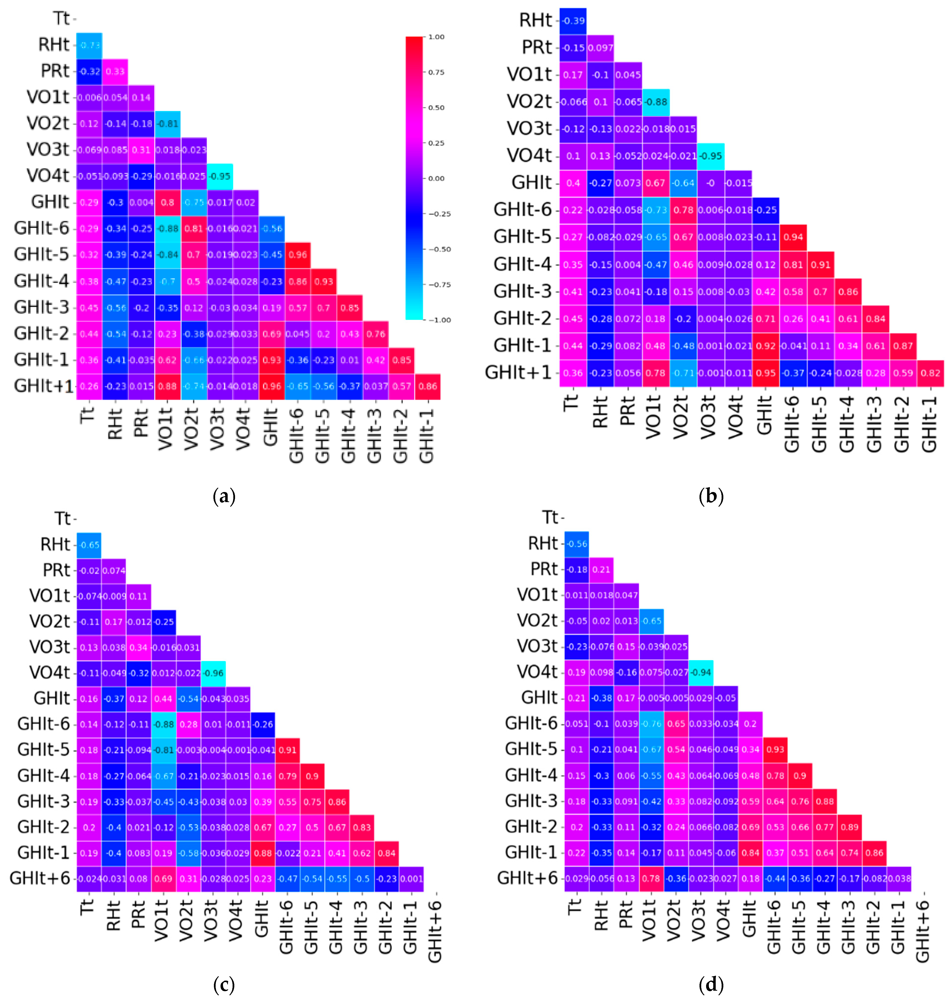
The Pearson and Spearman correlation coefficients are calculated between all variables. Thus, Figure 1 shows the results, using the Pearson coefficient, obtained for the two Algerian sites for t+1 and t+6 horizons and

Table 3. Ranking obtained using Pearson coefficient for all horizons and the two sites. Values indicate variable rankings, where 1 = most relevant and 14 = least relevant. The four first rankings were colored and made bold: red for the first, blue for the second, green for the third and orange for the fourth.

	Algiers						Ghardaïa
t+	+1	+2	+3	+4	+5	+6	+1	+2	+3	+4	+5	+6
GHIt	1	1	1	3	3	5	1	1	1	2	2	7
GHIt-1	9	3	4	4	8	13	2	3	3	5	9	10
GHIt-2	7	5	6	12	11	8	6	8	11	12	8	8
GHIt-3	5	10	12	10	7	7	12	11	8	7	6	6
GHIt-4	4	11	10	7	6	6	8	7	7	6	5	5
GHIt-5	11	9	8	6	5	4	7	6	5	4	4	3
GHIt-6	10	7	7	5	4	3	5	5	4	3	3	4
Tt	6	6	5	8	10	11	9	9	9	8	10	14
RHt	8	8	9	9	9	10	10	10	10	9	12	12
PRt	12	12	11	11	12	9	11	12	12	11	11	9
VO1t	2	2	2	1	1	1	3	2	2	1	1	1
VO2t	3	4	3	2	2	2	4	4	6	10	7	2
VO3t	14	14	14	14	14	12	14	14	14	14	14	11
VO4t	13	1.	13	13	13	14	13	13	13	13	13	13

presents the ranking of the inputs. As an illustration, the Pearson correlation coefficient between GHIt and GHIt–1 in Ghardaïa is higher than 0.9, indicating a strong linear relationship. This translates to a rank of 1 in Table 3.

The results obtained with the Spearman coefficient are shown in Figure 2 and given in

Table 4. Ranking obtained using Spearman coefficient for all horizons and the two sites. Values indicate variable rankings, where 1 = most relevant and 14 = least relevant. The four first rankings were colored and made bold: red for the first, blue for the second, green for the third and orange for the fourth.

	Algiers						Ghardaïa
t+	+1	+2	+3	+4	+5	+6	+1	+2	+3	+4	+5	+6
GHIt	1	1	2	3	5	6	1	1	2	2	6	7
GHIt-1	2	4	4	6	8	11	4	3	5	6	9	14
GHIt-2	5	5	8	12	12	9	6	8	11	10	8	8
GHIt-3	8	10	12	10	7	7	11	11	8	7	5	4
GHIt-4	12	11	9	7	6	5	8	7	6	5	4	2
GHIt-5	9	8	6	5	4	4	7	6	4	4	2	3
GHIt-6	6	6	5	4	3	2	5	5	3	3	3	5
Tt	7	7	7	8	9	12	9	9	9	8	10	13
RHt	10	9	10	9	10	10	10	10	10	9	11	10
PRt	11	12	11	11	11	8	12	13	14	13	12	9
VO1t	3	2	1	1	1	1	2	2	1	1	1	1
VO2t	4	3	3	2	2	3	3	4	7	14	7	6
VO3t	14	13	13	14	14	14	14	14	13	12	14	11
VO4t	13	14	14	13	13	13	13	12	12	11	13	12

.

In the context of the ranking tables (Table 3, Table 4,

Table 5. Ranking obtained using Mutual Information for all horizons and the two sites. Values indicate variable rankings, where 1 = most relevant and 14 = least relevant. The four first rankings were colored and made bold: red for the first, blue for the second, green for the third and orange for the fourth.

	Algiers						Ghardaïa
t+	+1	+2	+3	+4	+5	+6	+1	+2	+3	+4	+5	+6
GHIt	1	1	1	4	9	11	1	1	1	5	10	11
GHIt-1	2	3	5	10	11	10	2	4	7	11	11	10
GHIt-2	5	7	10	9	7	7	7	10	10	10	7	8
GHIt-3	8	10	8	7	6	5	9	9	9	7	5	4
GHIt-4	9	8	7	6	4	3	8	7	5	4	4	3
GHIt-5	7	6	6	5	5	4	6	5	4	3	2	2
GHIt-6	6	5	4	3	2	1	4	3	3	1	1	1
Tt	12	12	12	12	12	12	12	12	12	12	12	12
RHt	13	13	13	13	13	13	13	13	13	13	13	13
PRt	14	14	14	14	14	14	14	14	14	14	14	14
VO1t	3	2	2	1	1	2	3	2	2	2	3	6
VO2t	4	4	3	2	3	6	5	6	6	8	8	5
VO3t	10	9	9	8	8	8	10	8	8	6	6	7
VO4t	11	11	11	11	10	9	11	11	11	9	9	9

,

Table 6. Ranking of input variables by LASSO method for Solar Irradiance Forecasting (t+1 to t+6) in Ghardaïa and Algiers. Values indicate variable rankings, where 1 = most relevant and 14 = least relevant. The four first rankings were colored and made bold: red for the first, blue for the second, green for the third and orange for the fourth.

	Algiers						Ghardaïa
t+	+1	+2	+3	+4	+5	+6	+1	+2	+3	+4	+5	+6
GHIt	1	1	2	2	2	2	1	2	2	3	3	3
GHIt-1	14	14	14	14	14	14	14	14	14	14	14	14
GHIt-2	13	13	13	13	13	13	13	13	13	13	13	13
GHIt-3	12	12	12	12	12	12	12	12	12	12	12	12
GHIt-4	11	11	5	5	11	11	11	11	11	11	11	11
GHIt-5	10	10	11	11	10	10	10	10	10	10	10	10
GHIt-6	9	3	3	3	3	4	9	9	9	5	4	9
Tt	3	4	6	6	5	6	3	4	4	4	5	4
RHt	4	5	7	7	6	7	5	6	7	8	6	5
PRt	5	6	8	8	7	8	6	7	6	7	7	6
VO1t	2	2	1	1	1	1	2	1	1	1	1	1
VO2t	6	7	4	4	4	3	4	3	3	2	2	2
VO3t	7	8	9	9	8	5	7	5	5	6	8	7
VO4t	8	9	10	10	9	9	8	8	8	9	9	8

,

Table 7. Ranking of input variables by RFE-GB method for Solar Irradiance Forecasting (t+1 to t+6) in Ghardaïa and Algiers. Values indicate variable rankings, where 1 = most relevant and 14 = least relevant. The four first rankings were colored and made bold: red for the first, blue for the second, green for the third and orange for the fourth.

	Algiers						Ghardaïa
t+	+1	+2	+3	+4	+5	+6	+1	+2	+3	+4	+5	+6
GHIt	1	1	1	2	2	2	1	1	1	2	2	5
GHIt-1	10	4	4	4	4	10	3	4	4	4	4	6
GHIt-2	4	5	11	12	12	14	4	6	10	9	9	7
GHIt-3	5	10	10	11	11	13	9	13	9	5	5	12
GHIt-4	11	8	9	14	14	9	13	14	11	11	11	3
GHIt-5	12	12	12	9	9	8	14	10	6	7	7	4
GHIt-6	13	14	5	5	5	3	10	9	12	6	6	2
Tt	9	11	8	7	7	5	8	8	8	8	8	8
RHt	6	6	6	8	8	7	6	5	5	12	12	14
PRt	8	9	13	10	10	11	7	11	14	13	13	13
VO1t	2	2	2	1	1	1	2	2	2	1	1	1
VO2t	3	3	3	3	3	4	5	3	3	3	3	10
VO3t	7	7	7	6	6	6	12	7	13	14	14	9
VO4t	14	13	14	13	13	12	11	12	7	10	10	11

,

Table 8. Ranking of input variables by RFE-RF method for Solar Irradiance Forecasting (t+1 to t+6) in Ghardaïa and Algiers. Values indicate variable rankings, where 1 = most relevant and 14 = least relevant.

	Algiers						Ghardaïa
t+	+1	+2	+3	+4	+5	+6	+1	+2	+3	+4	+5	+6
GHIt	1	1	1	2	2	4	1	1	1	2	3	6
GHIt-1	4	4	7	4	5	9	3	4	4	4	7	11
GHIt-2	5	5	4	10	13	13	4	5	5	7	6	7
GHIt-3	7	9	11	12	10	12	7	11	7	6	10	10
GHIt-4	10	10	9	11	11	11	11	7	6	10	8	4
GHIt-5	11	8	12	7	9	8	9	9	10	8	5	3
GHIt-6	8	11	5	5	4	2	8	8	8	5	4	2
Tt	9	7	8	6	6	5	6	6	9	9	9	5
RHt	6	6	6	8	7	6	10	10	11	11	13	9
PRt	12	12	10	9	8	10	12	12	12	12	12	8
VO1t	2	2	2	1	1	1	2	2	2	1	1	1
VO2t	3	3	3	3	3	3	5	3	3	3	2	14
VO3t	13	13	13	13	12	7	13	13	13	13	11	12
VO4t	14	14	14	14	14	14	14	14	14	14	14	13

,

Table 9. Ranking of input variables by SHAP-GB method for Solar Irradiance Forecasting (t+1 to t+6) in Ghardaïa and Algiers. Values indicate variable rankings, where 1 = most relevant and 14 = least relevant. The four first rankings were colored and made bold: red for the first, blue for the second, green for the third and orange for the fourth.

	Algiers						Ghardaïa
t+	+1	+2	+3	+4	+5	+6	+1	+2	+3	+4	+5	+6
GHIt	1	1	1	2	2	3	1	1	1	2	2	3
GHIt-1	11	4	4	4	5	10	3	3	4	4	12	7
GHIt-2	4	5	10	11	14	14	4	5	9	10	5	6
GHIt-3	7	7	8	13	12	11	9	12	12	8	11	8
GHIt-4	8	9	12	12	11	12	13	14	8	12	10	5
GHIt-5	6	11	11	9	10	8	14	9	10	9	8	4
GHIt-6	14	14	5	5	4	4	8	11	11	6	4	2
Tt	12	10	7	6	8	9	7	8	7	5	14	9
RHt	9	8	6	7	7	13	6	6	5	13	7	14
PRt	10	12	13	10	9	7	12	13	14	11	13	13
VO1t	2	3	2	1	1	1	2	2	2	1	1	1
VO2t	3	2	3	3	3	2	5	4	3	3	3	12
VO3t	13	13	9	8	6	6	11	7	13	14	6	10
VO4t	5	6	14	14	13	5	10	10	6	7	9	11

and

Table 10. Ranking of input variables by SHAP-RF method for Solar Irradiance Forecasting (t+1 to t+6) in Ghardaïa and Algiers. Values indicate variable rankings, where 1 = most relevant and 14 = least relevant. The four first rankings were colored and made bold: red for the first, blue for the second, green for the third and orange for the fourth.

	Algiers						Ghardaïa
t+	+1	+2	+3	+4	+5	+6	+1	+2	+3	+4	+5	+6
GHIt	1	1	1	2	2	3	1	1	1	2	3	4
GHIt-1	7	5	7	6	6	8	4	3	4	5	5	8
GHIt-2	6	6	6	11	12	14	5	5	6	7	8	7
GHIt-3	8	13	11	12	14	13	9	11	10	10	10	10
GHIt-4	13	12	12	14	13	11	13	8	9	11	11	5
GHIt-5	11	10	14	10	11	10	8	10	12	9	6	3
GHIt-6	9	8	5	5	5	2	11	7	5	4	4	2
Tt	12	11	10	7	8	6	7	6	8	9	9	6
RHt	10	9	9	9	9	9	12	13	13	13	14	13
PRt	14	14	13	13	11	12	14	14	14	14	13	8
VO1t	2	2	2	1	1	1	2	2	2	1	1	1
VO2t	3	3	3	3	3	5	3	4	3	3	2	14
VO3t	4	7	8	8	7	7	10	9	7	6	7	10
VO4t	5	4	4	4	4	4	6	12	11	12	12	12

), lower rank numbers indicate higher feature relevance. These ranks are derived from the variable importance according to each selection method. They do not represent the actual correlation, Mutual Information, or coefficient values. Noticeable differences appear between the two stations. The results reveal strong dependencies between GHIt+h and recent values (GHIt, GHIt−1) for short-term horizons (t+1 to t+3), along with a consistent influence of the periodic variable VO1t across all horizons. These correlations weaken at longer horizons (t+4 to t+6), for which periodic variables (VO1t, VO2t) reflecting daily and seasonal cycles become more relevant. Atmospheric pressure (PRt) and temperature (Tt) show no significant correlation at either site. In Ghardaïa, the stable arid climate leads to consistently higher correlations for past GHIt across all horizons. In contrast, Algiers exhibits weaker correlations, reflecting its more variable Mediterranean climate. Consequently, GHIt values are the main input for short-term forecasts, while periodic variables help extend predictive capability over longer horizons, particularly in more variable climates like Algiers.

3.2. Mutual Information Analysis

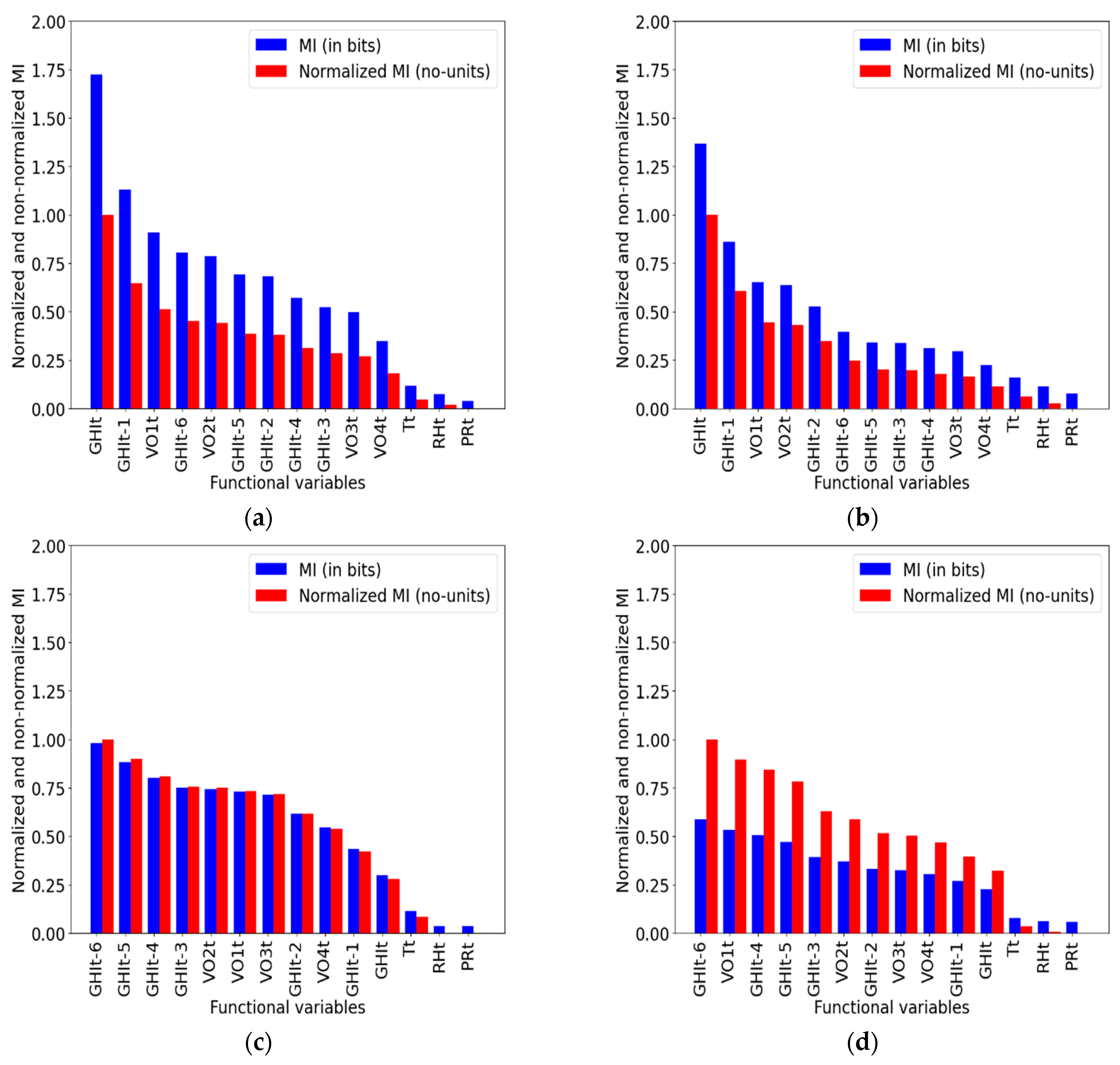
Mutual Information (MI) captures both linear and non-linear dependencies between GHIt+h (h = 1 to 6 h) and the inputs. Figure 3 shows bar plots of MI values (in bits) and normalized MI (dimensionless) for each input variable. At the same forecast horizon, bar height variability is greater for shorter horizons than for longer ones. This indicates that as the horizon increases, most inputs exhibit similar levels of influence, except for the weather parameters (temperature, humidity, and pressure), which remain negligible.

The results (in Table 5) reveal clear contrasts between Ghardaïa and Algiers: while, for both, past GHIt values dominate for short horizons, for longer horizons, in Algiers, periodic variables (VO1t, VO2t) gain relevance, while GHIt-5 and GHIt-6 are predominant in Ghardaïa. The ordinal value VO1 is still ranked in the top three most influential variables, which shows the importance that this very rarely used variable can have in predicting solar radiation. The three meteorological variables Tt, RHt, and PRt have a negligeable influence and will be not used as input in the forecasting model, regardless of the forecast horizon and the station considered. MI values are generally higher in Ghardaïa, indicating stronger input–target links and reflecting distinct climatic dynamics.

3.3. LASSO Analysis

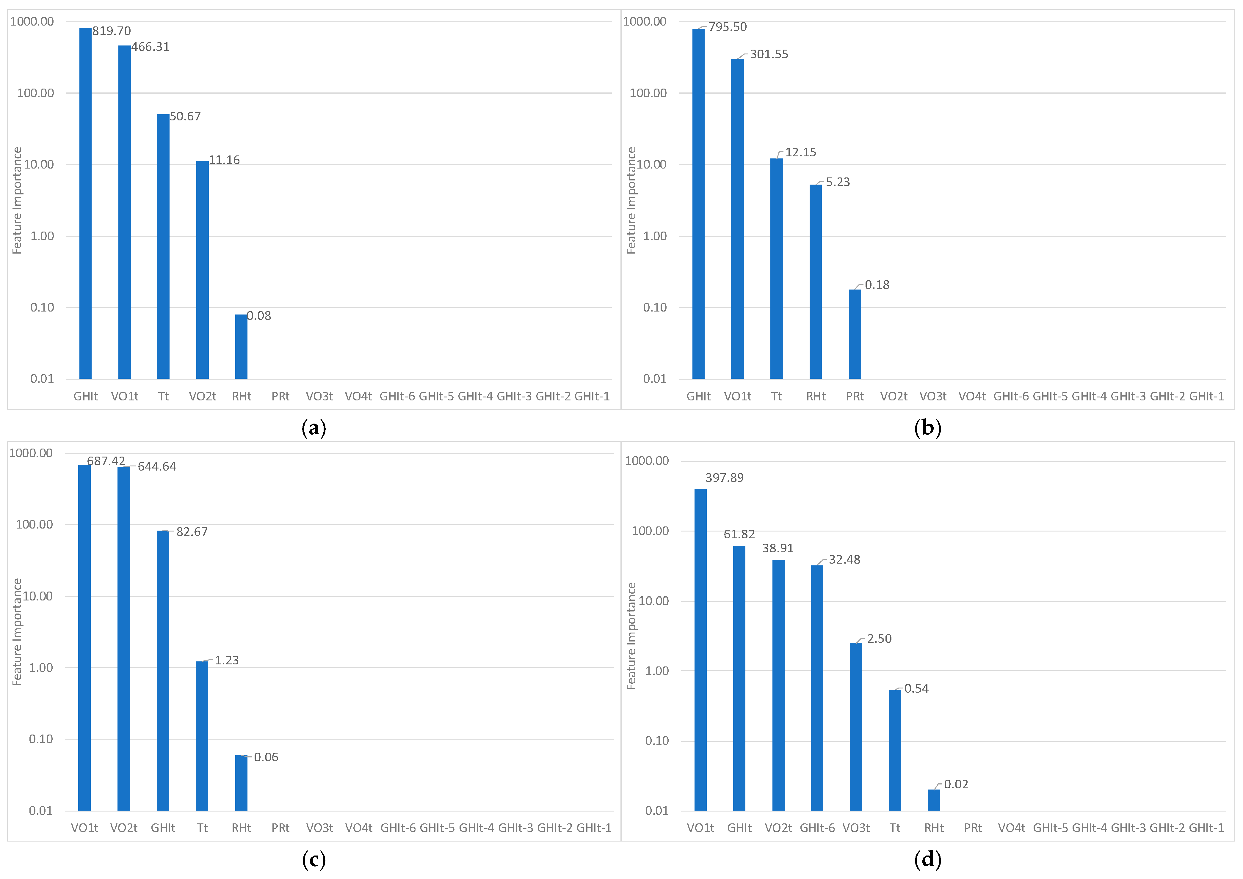
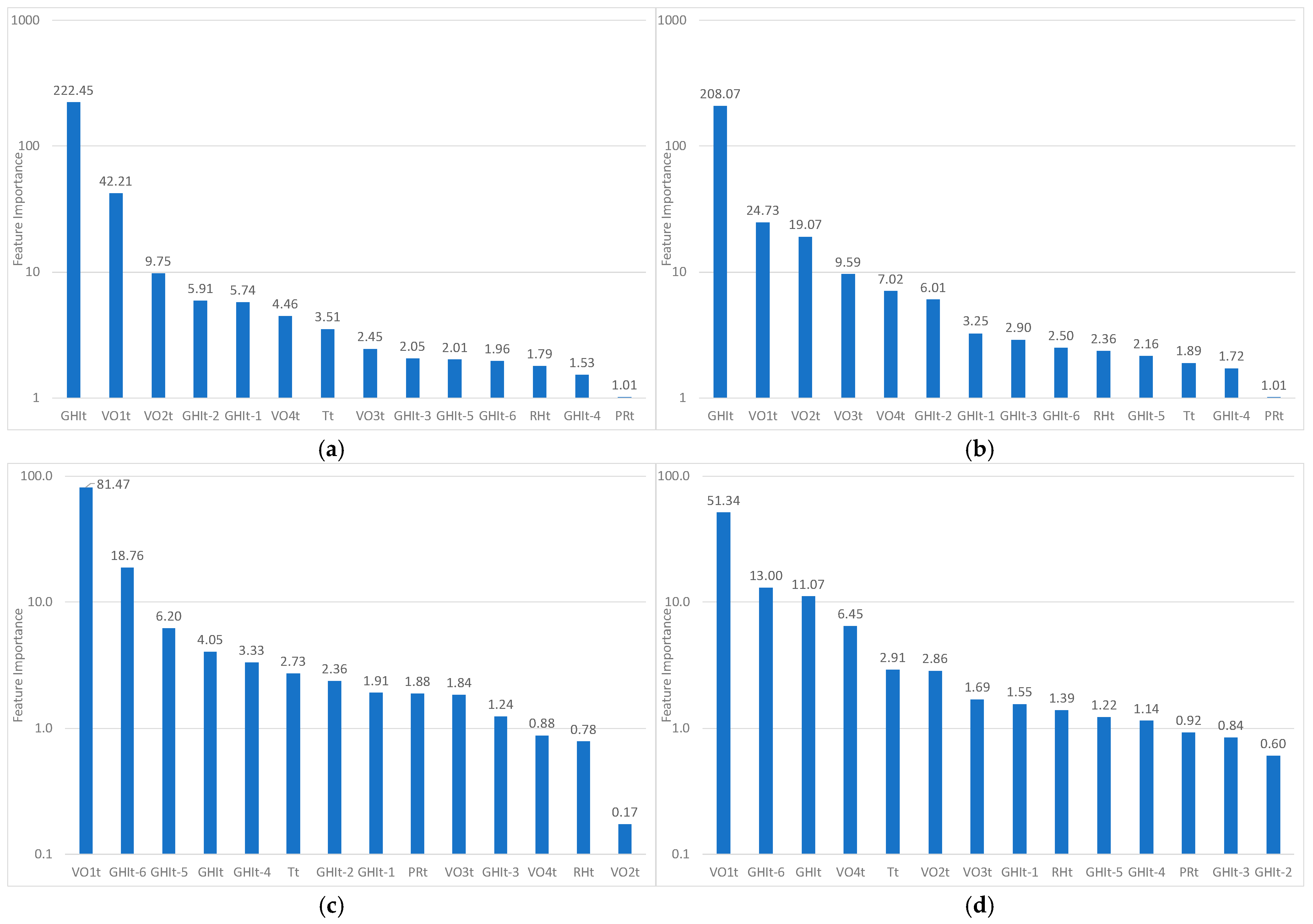
Lasso regression results (Figure 4) identify the key predictors of GHIt+h. Unlike with MI, LASSO reveals a few clearly dominant input variables. In Ghardaïa, 3 to 4 inputs typically dominate depending on the horizon, while in Algiers, usually only 2 or 3 variables stand out. For both stations, the number of predominant inputs increases with the forecast horizon.

The ranking of the inputs by the influence order identified by Lasso is presented in Table 6. For short-term horizons (t+1 to t+3), recent GHI values (GHIt) and the seasonal component VO1t consistently dominate in both Ghardaïa and Algiers. In Ghardaïa, Tt and VO2t also contribute modestly. As the horizon extends (t+4 to t+6), the influence of recent GHIt values declines (especially in Ghardaïa), while VO1t and VO2t gain importance, as already noted with the three previous methods. In Algiers, GHIt-6 appears more frequently but remains less influential. For long-term forecasts, GHIt, VO1t, and VO2t are the most important in Ghardaïa, whereas in Algiers, VO2t is replaced by GHIt-6. Most other variables show a negligible impact, with near-zero coefficients. Temperature (Tt), while occasionally selected, plays a minor role, which is slightly more pronounced in Ghardaïa.

3.4. RFE Analysis

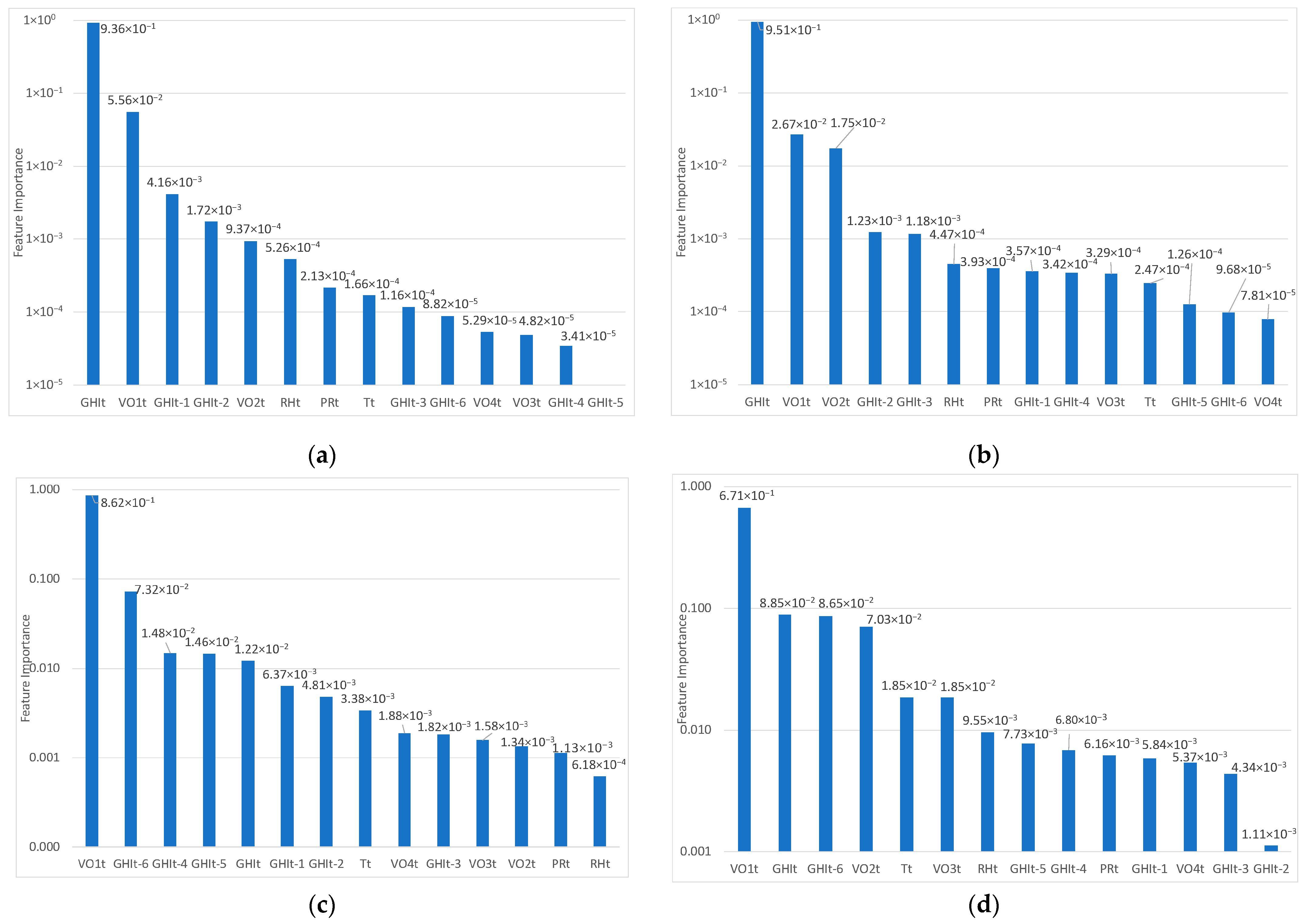
Figure 5 and Figure 6 present the feature importance rankings from RFE-GB and RFE-RF models across all forecasting horizons (h = 1 and 6). RFE iteratively removes the least important features to identify the optimal subset per horizon. As with LASSO, only two or three inputs show significant importance; beyond the third or fourth, their influence becomes negligible. This finding is important for determining the number of input variables to retain in the forecasting model.

The rankings are summarized in Table 7 and Table 8 for RFE-GB and RFE-RF, respectively.

Concerning the ranking of the input variables for each horizon, it is different for the RFE-GB and RFE-RF selection methods, even if the differences are not very important. However, as noted in the previous method, across all horizons and both sites GHIt and VO1t consistently rank as the top predictors, with GHIt-1 and VO2t frequently completing the top four. As the horizon increases (t+4 to t+6), GHIt contribution declines. Meteorological variables (Tt, RHt, PRt) play a secondary role, as seen with previous selection methods. Both models confirm GHIt as the most relevant variable for short-term horizons, while periodic features become essential for longer-term forecasts.

3.5. SHAP Analysis

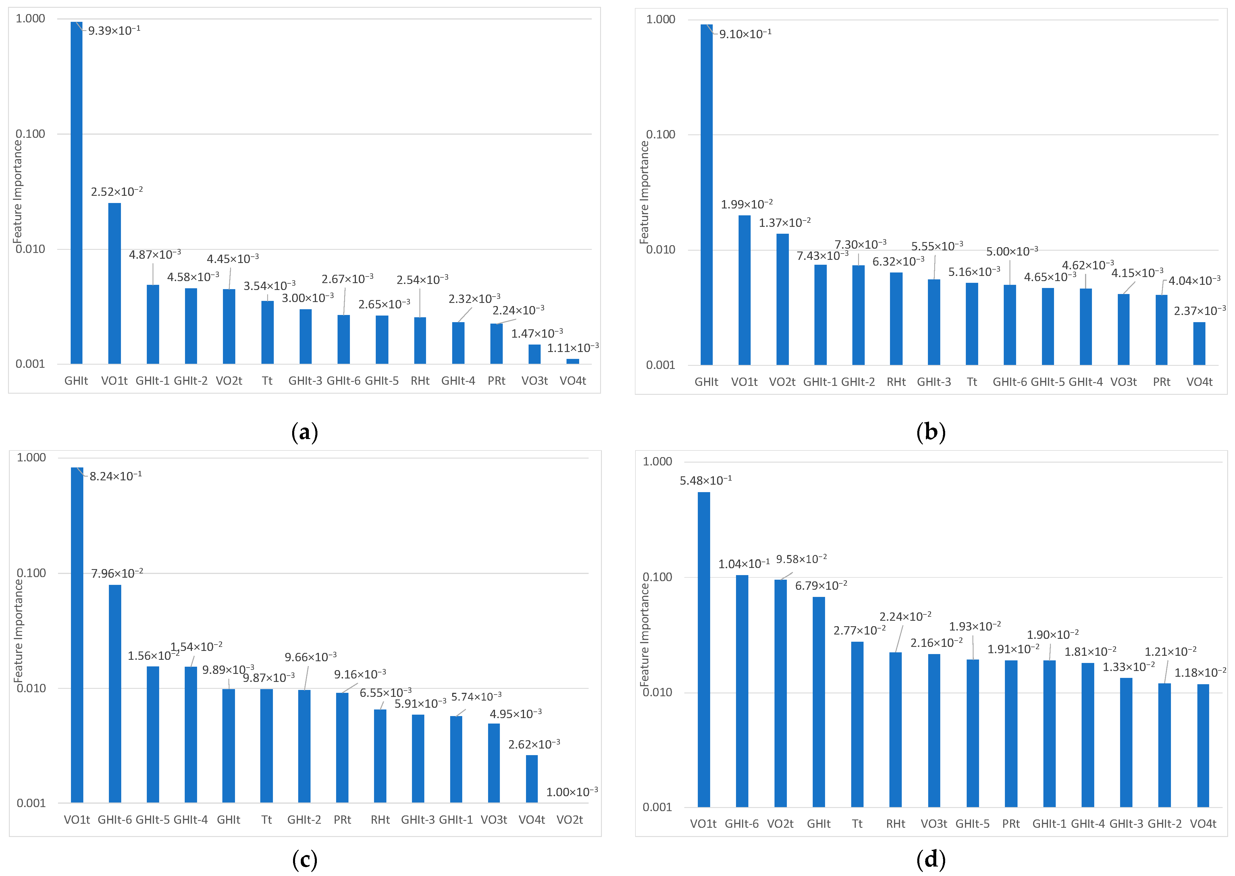
Figure 7 and Figure 8 present the importance of the functional variables as assessed by SHAP (SHapley Additive exPlanations) values, which quantify the contribution of each variable regarding predictions. Figure 7 corresponds to the Gradient Boosting (GB) model, while Figure 8 refers to the Random Forest (RF) model. As the forecast horizon increases, the strength of input–output link tends to decline. As previously noted, from the third or fourth input, the level of connection between input and output becomes very weak and it is certainly not necessary to use more than four inputs to operate predictions. The ranking of the input variables according to SHAP-GB and SHAP-RF are presented in Table 9 and Table 10. From horizons t+1 to t+3, the SHAP analysis applied to the Gradient Boosting model highlights GHIt as the most influential predictor for both Ghardaïa and Algiers. For Ghardaïa, GHIt, VO1t, and GHIt-1 show the highest contributions, while for Algiers, GHIt-1 is replaced by VO2t. Concerning intermediate horizons (t+3 and t+4), the importance of VO2t increases in Ghardaïa, complementing the previously dominant predictors. At t+4 to t+6, the contribution of past GHIt values decrease, periodic variables (VO1t) mainly dominate, andGHIt-6 emerges as a key predictor for both sites. This suggests a shift in dependence toward older lagged inputs as the forecast horizon increases. In the Random Forest framework, the model progressively relies on the full set of cyclical predictors, and as the prediction horizon increases, the model relies more on cyclical variables and longer GHIt lags. Once again, the ordinal variables (especially VO1t) prove to be highly influential.

3.6. Comparison of the Results Obtained by the Eight Selection Methods

Some general remarks can be made, which are applicable to all selection methods and stations:

• As the forecast horizon increases, input–output correlations weaken;
• Most methods suggest that only three or four variables meaningfully correlate with the output (though not always the same ones);
• Some variables are consistently ranked low and will therefore be excluded from the forecasting inputs in the next section.

For short-term horizons (t+1 to t+3), all models identify historical GHI values (GHIt, GHIt−1) as the dominant predictors, particularly in Ghardaïa due to its stable climate. For intermediate horizons, periodic components (VO1t, VO2t) gain importance. These ordinal variables are consistently ranked highly, despite being rarely used in solar radiation forecasting methods, which confirms the conclusions in [42]; VO3t and VO4t are much less relevant variables. RF and GB handle these non-linear interactions better than LASSO, which is limited by its linear nature. For long-term horizons (t+5, t+6), RF and GB emphasize periodic variables and past GHI values, while LASSO focuses more on temperature (T). In summary, LASSO provides simplicity and interpretability for short-term forecasts, while RF and GB are more effective at modeling non-linear relationships, especially at longer horizons. The complexity of the methods varies significantly:

• Correlation and MI analyses are computationally simple, providing valuable initial insights into feature relevance but lacking the ability to model feature interactions;
• RFE is more computationally intensive but provides robust feature rankings by leveraging ensemble methods such as RF and GB (similar results), making it suitable for datasets with complex dependencies;
• LASSO Regression strikes a balance between simplicity and efficiency, making it ideal for scenarios where interpretability and speed are important;
• SHAP offers the most detailed insights, quantifying the contributions of each feature while addressing non-linear interactions. However, it requires substantial computational resources and advanced interpretative tools.

Statistical links between inputs and output tends to drop significantly beyond the third or fourth ranked variable. Consequently, only the first four variables retained by each method, for each site and each horizon, will be used as input for the forecast test.

Table 11. The first four variables selected as inputs according to the four selection methods for each time step and meteorological station. The boxes are highlighted in red for the one in first position, blue for the second, green for the third, and orange for the fourth.

Horizon	t+1																t+2
Station	Algiers								Ghardaïa								Algiers								Ghardaïa
Method *	1	2	3	4	5	6	7	8	1	2	3	4	5	6	7	8	1	2	3	4	5	6	7	8	1	2	3	4	5	6	7	8
GHIt
GHIt-1
GHIt-2
GHIt-3
GHIt-4
GHIt-5
GHIt-6
Tt
RHt
PRt
VO1t
VO2t
VO3t
VO4t
Horizon	t+3																t+4
Station	Algiers								Ghardaïa								Algiers								Ghardaïa
Method	1	2	3	4	5	6	7	8	1	2	3	4	5	6	7	8	1	2	3	4	5	6	7	8	1	2	3	4	5	6	7	8
GHIt
GHIt-1
GHIt-2
GHIt-3
GHIt-4
GHIt-5
GHIt-6
Tt
RHt
PRt
VO1t
VO2t
VO3t
VO4t
Horizon	t+5																t+6
Station	Algiers								Ghardaïa								Algiers								Ghardaïa
Method	1	2	3	4	5	6	7	8	1	2	3	4	5	6	7	8	1	2	3	4	5	6	7	8	1	2	3	4	5	6	7	8
GHIt
GHIt-1
GHIt-2
GHIt-3
GHIt-4
GHIt-5
GHIt-6
Tt
RHt
PRt
VO1t
VO2t
VO3t
VO4t

* 1. Pearson; 2. Spearman; 3. Mutual Information; 4. LASSO; 5. RFE-GB; 6. RFE-RF; 7. SHAP-GB; 8. SHAP-RF.

summarizes, for the two meteorological sites and each horizon, the four retained variables; they are highlighted in red for the one in first position, blue for the second, green for the third, and orange for the fourth.

Thanks to this representation (Table 11), the comparison of the four inputs selected using each method is easier. It is observed that:

• The ordinal value VO1 always belongs to the quartet of inputs, except for one case, and is, most of the time, in first or second position: second position for horizons t+1 to t+3 for Algiers and Ghardaïa and first position for longer horizons (t+4 to t+6);
• GHIt is preponderant for predicting GHIt+1 and GHIt+2, irrespective of the station;
• GHIt-1 gradually disappears with increasing forecast horizon;
• Meteorological variables (Tt, RHt, PRt) were rarely selected, confirming their limited relevance for short-term forecasting in the studied climates.

VO2t gained importance at longer horizons, complementing VO1t in capturing diurnal patterns. GHIt-6 occasionally appeared beyond t+4, suggesting some residual value from distant lags. Overall, the convergence of methods on compact input sets validates the use of three to four variables without compromising accuracy. Despite methodological diversity, most techniques converge in identifying historical GHI as critical for short-term forecasts, and periodic variables for extended horizons. The next section evaluates whether these insights hold when applying a GB forecasting model using each feature subset.

4. Forecasting Algorithm Application and Comparison of Performance of Selection Methods

To assess the relevance of each feature selection method, the four input variables retained for each method (Table 11) were used in a Gradient Boosting (GB) model, chosen for its robustness and proven performance in solar forecasting tasks. Performance was assessed using normalized Mean Absolute Error (nMAE) and normalized Root Mean Square Error (nRMSE). It should be noted that the exclusion of meteorological variables (e.g., temperature, humidity, pressure) in most selection outcomes is the result of data-driven procedures and is not based on manual judgment. While these features showed limited relevance in the specific climatic conditions of Algiers and Ghardaïa, they may be more informative in different geographical contexts or under seasonal extremes. Therefore, feature selection results should be interpreted with respect to the local environment and forecasting objectives.

Table 12. Comparison of nMAE and nRMSE (%) in hourly GHI forecasting with selected inputs by each feature selection method (the best results for each time horizon are in red bold, second-best result in blue, and worst result in purple bold).

Forecasting Horizon	Method Number	GHARDAÏA		ALGIERS
		nMAE (%)	nRMSE (%)	nMAE (%)	nRMSE (%)
t+1	1	6.52	12.05	11.13	18.00
	2	6.52	12.05	11.57	18.20
	3	6.44	11.93	11.57	18.20
	4	6.62	12.08	10.82	17.97
	5	6.48	12.04	11.40	18.03
	6	6.48	12.04	11.57	18.20
	7	6.48	12.04	11.40	18.03
	8	6.52	12.05	11.84	18.53
t+2	1	9.33	15.54	17.88	27.50
	2	9.33	15.54	17.88	27.50
	3	9.14	15.40	17.88	27.50
	4	9.00	15.36	17.50	27.00
	5	9.33	15.54	17.88	27.50
	6	9.33	15.54	17.88	27.50
	7	9.33	15.54	17.88	27.50
	8	9.33	15.54	20.38	28.63
t+3	1	11.12	18.37	22.44	34.45
	2	11.10	18.22	22.44	34.45
	3	11.10	18.22	21.28	32.82
	4	11.48	19.16	21.28	32.82
	5	11.44	19.13	22.44	34.45
	6	11.44	19.13	23.01	34.62
	7	11.44	19.13	22.44	34.45
	8	11.44	19.13	24.26	34.78
t+4	1	13.60	22.00	26.23	27.20
	2	13.60	22.00	23.60	35.34
	3	11.12	18.37	23.60	35.34
	4	14.48	23.34	23.60	35.34
	5	14.80	23.50	26.23	37.20
	6	14.80	23.50	26.23	37.20
	7	14.80	23.50	26.23	37.20
	8	13.70	22.35	27.66	37.80
t+5	1	17.00	27.62	25.84	35.83
	2	18.50	30.00	28.40	37.90
	3	18.50	30.00	27.65	36.77
	4	16.83	27.00	25.84	35.83
	5	16.92	27.23	25.45	35.70
	6	16.83	27.00	25.84	35.83
	7	16.83	27.00	25.84	35.83
	8	16.83	27.00	28.00	39.21
t+6	1	19.00	31.15	31.28	42.00
	2	20.84	32.80	32.28	42.00
	3	19.52	31.62	31.00	41.73
	4	22.37	33.27	28.52	40.23
	5	19.25	31.44	28.13	39.64
	6	19.25	31.44	28.52	40.23
	7	17.17	28.30	28.52	40.23
	8	17.17	28.30	31.12	41.96

1: Pearson; 2: Spearman, 3: MI; 4: LASSO; 5: RFE-GB; 6: RFE-RF; 7: SHAP-GB; 8: SHAP-RF.

presents error values for each method across six forecasting horizons. The errors metrics are computed as follows:

$$\mathrm{n}\mathrm{M}\mathrm{A}\mathrm{E}={\displaystyle \frac{100}{N}}{\sum }_{i=1}^N{\displaystyle \frac{\left|{\widehat{y}}_i-y_i\right|}{\overline{y}}}$$

(10)

$$nRMSE={\displaystyle \frac{100}{\sqrt{N}}}\sqrt{{\sum }_{i=1}^N{\displaystyle \frac{{({\widehat{y}}_i-y_i)}^2}{\overline{y}}}}$$

(11)

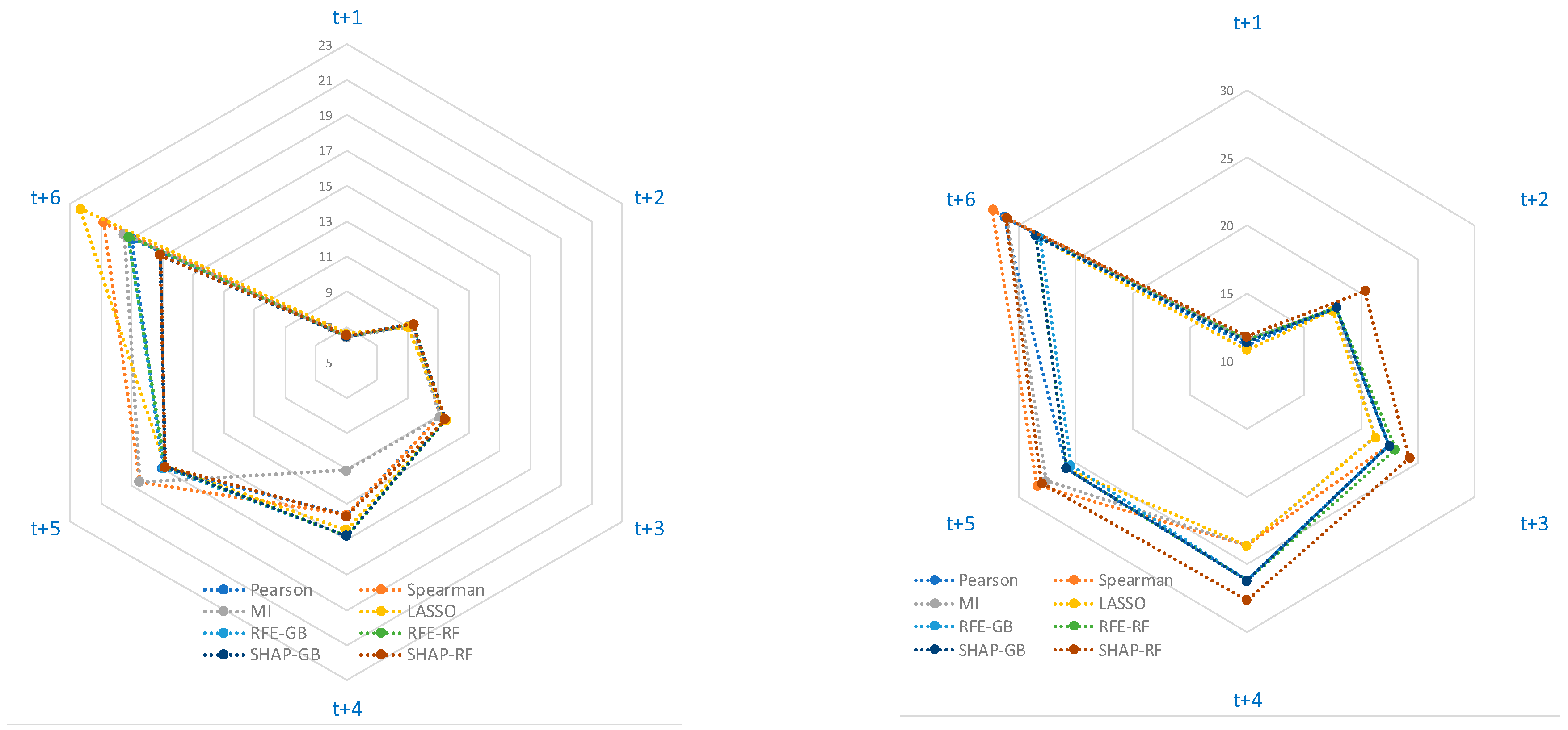
where ${\widehat{y}}_i$ is the predicted GHI, $y_i$ the observed GHI, and $\overline{y}$ the mean of observed GHI values over the test set of size N. As an example, for Ghardaïa at horizon t+1 with Mutual Information (Method 3), an nMAE of 6.44% means that the average absolute error represents 6.44% of the average measured GHI over the evaluation period.

Table 13. Best Feature Selection Method per Forecast Horizon and Site (based on nMAE).

Forecast Horizon	Ghardaïa–Best Method (nMAE%)	Algiers–Best Method (nMAE%)
t+1	Mutual Information (6.44%)	LASSO (10.82%)
t+2	LASSO (9.00%)	LASSO (17.50%)
t+3	Mutual Information (11.10%)	Mutual Information/LASSO (21.28%)
t+4	Mutual Information (11.12%)	Pearson/LASSO/MI (23.60%)
t+5	LASSO (16.83%)	RFE-GB (25.45%)
t+6	SHAP-GB/SHAP-RF (17.17%)	RFE-GB (28.13%)

summarizes the best-performing feature selection method for each forecast horizon and meteorological site, based on the lowest nMAE values. For Ghardaïa, Mutual Information and SHAP-based approaches dominate, particularly at short and long horizons, respectively. In Algiers, LASSO yields consistent performance up to t+4, while RFE-GB outperforms others at longer horizons. This summary may serve as a practical reference for practitioners tailoring forecasting models to specific climatic contexts and timeframes. Figure 9 shows radar plots of nMAE for Ghardaïa and Algiers (nRMSE plots are omitted due to similar feature rankings). The results indicate consistently lower errors in Ghardaïa, reflecting its more stable arid climate.

At short forecast horizons (e.g., t+1), most methods show similar performance, with only small differences in nMAE (e.g., 6.44% vs. 6.52% in Ghardaïa). However, even such small differences can be meaningful in operational contexts such as energy dispatch. As the forecast horizon increases, performance gaps between methods become more pronounced, with relative improvements reaching 10–30%, highlighting the growing impact of feature selection. This trend is also confirmed by the overall increase in nMAE and nRMSE values with time, reflecting the decreasing accuracy of predictions at extended horizons. Prediction errors are consistently higher for Algiers than for Ghardaïa, likely due to greater solar radiation variability, which increases forecasting complexity. In Ghardaïa, the Mutual Information method produced the most accurate forecasts at short-term horizons, with the lowest nMAE values at t+1 (6.44%) and t+4 (11.12%). In Algiers, LASSO consistently performed well across all horizons, achieving the best nMAE at t+1 (10.82%) and maintaining strong results up to t+6. Conversely, LASSO was less effective in Ghardaïa. SHAP- and RFE-based methods showed more mixed results: while they outperformed other approaches at longer horizons in Ghardaïa (particularly at t+6, with SHAP-GB and SHAP-RF both reaching nMAE = 17.17%), they were less competitive for short-term forecasts. It is worth examining whether the choice of input variables significantly influences forecast accuracy. This influence selection becomes more evident at longer horizons. In Ghardaïa, its impact is limited at t+1, with a gain of 0.18 percentage points (a 2.79% improvement in nMAE), but increases significantly by t+6, reaching 5.2 percentage points (a 30.28% improvement). In Algiers, the impact of feature selection is also evident at horizon t+6. The best performance is achieved with RFE-GB (nMAE = 28.13%), while the worst comes from Spearman-based selection (nMAE = 32.28%), yielding an improvement of 4.15% points, or 12.86% relative. To statistically assess the influence of input selection methods on forecast accuracy, we applied the Wilcoxon signed-rank test to compare the best- and worst-performing methods across all horizons. The results show that in Ghardaïa, differences in performance are not statistically significant (p > 0.2), which may be due to the lower variability in solar radiation. In contrast, in Algiers, the difference is significant for nMAE (p = 0.031) and near-significant for nRMSE (p = 0.063), confirming that input selection plays a more critical role under more variable conditions.

Lower values indicate better performance. For Ghardaïa, methods converge at short horizons but diverge at longer ones, with SHAP-based approaches showing the lowest errors at t+6. In Algiers, differences are less marked, though LASSO and RFE-GB perform slightly better overall. Overall, although feature selection has a growing impact at extended horizons, the performance differences between methods remain moderate. This indicates that simpler selection techniques may still yield competitive results, depending on the forecasting context and local climate conditions.

Summary of Forecasting Results: Forecasting accuracy degrades as the prediction horizon increases, with both nMAE and nRMSE values rising accordingly. At short horizons (e.g., t+1), all feature selection methods perform comparably. However, performance gaps widen significantly from t+4 onward, particularly in Ghardaïa, where SHAP- and RFE-based methods outperform others at t+6. Mutual Information leads at t+1, reflecting its strength in capturing short-term dependencies. In Algiers, a more variable site, LASSO proves the most consistent across all horizons. To assess whether these differences are statistically meaningful, Wilcoxon signed-rank tests were applied. The results show that differences in nMAE are statistically significant in Algiers (p = 0.031) but not in Ghardaïa or for nRMSE. This suggests that feature selection influences average forecast accuracy (nMAE) most in climatically unstable environments, while error dispersion (nRMSE) remains less sensitive to the method used. For solar engineers, these results imply that advanced feature selection is especially beneficial:

• At longer horizons, where predictive complexity increases;
• In sites with high solar variability, where precision is more difficult to achieve;
• When the priority is to minimize systematic errors (nMAE), relevant for energy dispatch and storage decisions.

These findings support the use of feature selection strategies depending on the forecast horizon, site characteristics, and operational goals.

5. Conclusions

This study investigated feature selection for solar irradiance forecasting in two contrasting Algerian climates: Ghardaïa (arid) and Algiers (Mediterranean). The results show that the relevance of input variables (and the most effective selection method) depends strongly on both the forecast horizon and the local climate. The analysis covered a range of techniques, including correlation-based approaches (Pearson and Spearman), Mutual Information, LASSO, Recursive Feature Elimination (RFE), and SHAP. While all the methods yielded similar performance at short horizons, their effectiveness varied with time horizon and site, and no single method consistently outperformed the others. In terms of variable importance, a clearer picture emerges. Most methods agree on the central role of GHIt (irradiance at forecast launch) for short-term horizons and the growing importance of periodic variables such as VO1t and VO2t for longer horizons. Some lagged variables, like GHIt–6, also become relevant as the forecast extends. Interestingly, the ordinal variable VO1t (rarely used in forecasting literature) proved consistently useful across stations and methods, though its generalizability should be tested further in locations with greater solar variability. The added value of feature selection becomes more pronounced as the forecast horizon increases. For instance, while the gain in nMAE from optimal feature selection is limited to +2.79% at t+1 in Ghardaïa, it reaches +30.28% at t+6. In Algiers, the relative improvement ranges from +9.43% to +12.86% across the same horizons. Despite this, differences between selection methods remain moderate, indicating that simpler techniques such as Mutual Information or LASSO can be sufficient when appropriately tailored to the forecasting context. As an outlook, applying a deseasonalized formulation using the clear-sky index could reduce the dominance of periodic variables like VO1 and VO2.

However, this approach introduces challenges related to timestamp accuracy and the reliability of the clear-sky model itself, which may affect forecast consistency and generalizability. Moreover, this study is limited to two Algerian sites, chosen for their distinct climatic conditions. Extending the analysis to only a few more locations would increase the complexity without providing statistically meaningful generalization. A more robust validation would require access to consistent data from a larger network (e.g., 15–20 sites), which is not currently available in the region. In addition, the forecasting model used in this study (Gradient Boosting) was chosen for its balance between predictive performance, computational simplicity, and interpretability, particularly its compatibility with feature selection techniques such as SHAP or RFE. While deep learning methods (e.g., attention-based models) offer alternative strategies, a comprehensive and fair benchmarking of such architectures lies beyond the scope of this study. Finally, while the accuracy of forecasts is evaluated in statistical terms (nMAE, nRMSE), their downstream impact (such as economic benefits for energy dispatch, storage optimization, or grid management) has not been quantified here. Future research should address these limitations by expanding the geographical scope, comparing forecasting architectures, and integrating prediction outputs into operational or economic decision-making models.

References

1. Paletta, Q.; Terrén-Serrano, G.; Nie, Y.; Li, B.; Bieker, J.; Zhang, W.; Dubus, L.; Dev, S.; Feng, C. Advances in Solar Forecasting: Computer Vision with Deep Learning. Adv. Appl. Energy 2023, 11, 100150. [Google Scholar] [CrossRef]
2. Yang, D.; Wu, E.; Kleissl, J. Operational Solar Forecasting for the Real-Time Market. Int. J. Forecast. 2019, 35, 1499–1510. [Google Scholar] [CrossRef]
3. Stull, R.B. An Introduction to Boundary Layer Meteorology; Springer Science & Business Media: Berlin/Heidelberg, Germany, 1988. [Google Scholar] [CrossRef]
4. Notton, G.; Nivet, M.L.; Voyant, C.; Paoli, C.; Darras, C.; Motte, F.; Fouilloy, A. Intermittent and Stochastic Character of Renewable Energy Sources: Consequences, Cost of Intermittence and Benefit of Forecasting, Renew. Sustain. Energy Rev. 2018, 87, 96–105. [Google Scholar] [CrossRef]
5. Sobri, S.; Koohi-Kamali, S.; Rahim, N.A. Solar Photovoltaic Generation Forecasting Methods: A Review. Energy Conv. Manag. 2018, 156, 459–497. [Google Scholar] [CrossRef]
6. Jackson, I.; Ivanov, D.; Dolgui, A.; Namdar, J. Generative Artificial Intelligence in Supply Chain and Operations Management: A Capability-Based Framework for Analysis and Implementation. Int. J. Prod. Res. 2024, 62, 6120–6145. [Google Scholar] [CrossRef]
7. Sarbu, N.A.; Petreus, D.; Szilagyi, E. Practical Solutions for Microgrid Energy Management: Integrating Solar Forecasting and Correction Algorithms. Energy Rep. 2024, 12, 4160–4174. [Google Scholar] [CrossRef]
8. Kaur, A.; Nonnenmacher, L.; Pedro, H.T.C.; Coimbra, C.F.M. Benefits of Solar Forecasting for Energy Imbalance Markets. Renew. Energy 2016, 86, 819–830. [Google Scholar] [CrossRef]
9. Gandhi, O.; Zhang, W.; Kumar, D.S.; Rodríguez-Gallegos, C.D.; Yagli, G.M.; Yang, D.; Reindl, T.; Srinivasan, D. The Value of Solar Forecasts and the Cost of their Errors: A Review. Renew. Sustain. Energy Rev. 2024, 189 Pt B, 113915. [Google Scholar] [CrossRef]
10. Inman, R.H.; Pedro, H.T.C.; Coimbra, C.F.M. Solar Forecasting Methods for Renewable Energy Integration. Sol. Energy 2014, 105, 658–678. [Google Scholar] [CrossRef]
11. Krishnan, N.; Kumar, K.R.; Inda, C.S. How Solar Radiation Forecasting Impacts the Utilization of Solar Energy: A Critical Review. J. Clean. Prod. 2023, 388, 135860. [Google Scholar] [CrossRef]
12. Voyant, C.; Notton, G.; Kalogirou, S.A.; Nivet, M.L.; Paoli, C.; Motte, F.; Fouilloy, A. Machine Learning Methods for Solar Irradiance Time-Series Forecasting: A Review. Renew. Energy 2017, 105, 569–582. [Google Scholar] [CrossRef]
13. Kumari, P.; Toshniwal, D. Deep Learning Models for Solar Irradiance Forecasting: A Comprehensive Review. J. Clean. Prod. 2023, 318, 113226. [Google Scholar] [CrossRef]
14. Benti, N.E.; Chaka, M.D.; Semie, A.G. Forecasting Renewable Energy Generation with Machine Learning and Deep Learning: Current Advances and Future Prospects. Sustainability 2023, 15, 7087. [Google Scholar] [CrossRef]
15. Ying, C.; Wang, W.; Yu, J.; Li, Q.; Yu, D.; Liu, J. Deep Learning for Renewable Energy Forecasting: A Taxonomy, and Systematic Literature Review. J. Clean. Prod. 2023, 384, 135414. [Google Scholar] [CrossRef]
16. Jebbor, I.; Benmamoun, Z.; Hachimi, H. Forecasting Supply Chain Disruptions in the Textile Industry using Machine Learning: A Case Study. Ain Shams Eng. J. 2024, 15, 103116. [Google Scholar] [CrossRef]
17. Haqqi, M.; Benmamoun, Z.; Hachimi, H.; Raouf, Y.; Jebbor, I.; Akikiz, M. Renewable and Sustainable Energy: Solar Energy and Electrical System Design. In Proceedings of the 2023 9th International Conference on Optimization and Applications (ICOA), Abu Dhabi, United Arab Emirates, 5–6 October 2023; pp. 1–6. [Google Scholar]
18. Shakhovska, N.; Medykovskyi, M.; Gurbych, O.; Mamchur, M.; Melnyk, M. Enhancing Solar Energy Production Forecasting Using Advanced Machine Learning and Deep Learning Techniques: A Comprehensive Study on the Impact of Meteorological Data. Comput. Mater. Contin. 2024, 81, 3147–3163. [Google Scholar] [CrossRef]
19. Dhal, P.; Azad, C. A Comprehensive Survey on Feature Selection in the Various Felds of Machine Learning. Appl. Intell. 2022, 52, 4543–4581. [Google Scholar] [CrossRef]
20. Theng, D.; Bhoyar, K.K. Feature Selection Techniques for Machine Learning: A Survey of More than Two Decades of Research. Knowl. Inf. Syst. 2024, 66, 1575–1637. [Google Scholar] [CrossRef]
21. Xie, J.; Sage, M.; Fiona Zhao, Y. Feature Selection and Feature Learning in Machine Learning Applications for Gas Turbines: A Review. Eng. Appl. Artif. Intell. 2023, 117 Pt A, 105591. [Google Scholar] [CrossRef]
22. Salcedo-Sanz, S.; Cornejo-Bueno, L.; Prieto, L.; Paredes, D.; García-Herrera, R. Feature Selection in Machine Learning Prediction Systems for Renewable Energy Applications. Renew. Sustain. Energy Rev. 2018, 90, 728–741. [Google Scholar] [CrossRef]
23. Lyu, C.; Eftekharnejad, S.; Basumallik, S.; Xu, C. Dynamic Feature Selection for Solar Irradiance Forecasting Based on Deep Reinforcement Learning. IEEE Trans. Ind. Appl. 2023, 59, 533–543. [Google Scholar] [CrossRef]
24. Gao, Y.; Li, P.; Yang, H.; Wang, J. A Solar Radiation Intelligent Forecasting Framework based on Feature Selection and Multivariable Fuzzy Time Series. Eng. Appl. Artif. Intell. 2023, 126 Pt C, 106986. [Google Scholar] [CrossRef]
25. Surakhi, O.; Zaidan, M.A.; Fung, P.L.; Hossein Motlagh, N.; Serhan, S.; AlKhanafseh, M.; Ghoniem, R.M.; Hussein, T. Time-Lag Selection for Time-Series Forecasting using Neural Network and Heuristic Algorithm. Electronics 2021, 10, 2518. [Google Scholar] [CrossRef]
26. Solano, E.S.; Dehghanian, P.; Affonso, C.M. Solar Radiation Forecasting Using Machine Learning and Ensemble Feature Selection. Energies 2022, 15, 7049. [Google Scholar] [CrossRef]
27. Nematirad, R.; Pahwa, A. Solar Radiation Forecasting Using Artificial Neural Networks Considering Feature Selection. In Proceedings of the 2022 IEEE Kansas Power and Energy Conference (KPEC), Manhattan, KS, USA, 25–26 April 2022; pp. 1–4. [Google Scholar] [CrossRef]
28. Jebli, I.; Belouadha, F.Z.; Issam Kabbaj, M.; Tilioua, A. Prediction of Solar Energy Guided by Pearson Correlation Using Machine Learning. Energy 2021, 224, 120109. [Google Scholar] [CrossRef]
29. Fraihat, H.; Almbaideen, A.A.; Al-Odienat, A.; Al-Naami, B.; De Fazio, R.; Visconti, P. Solar Radiation Forecasting by Pearson Correlation Using LSTM Neural Network and ANFIS Method: Application in the West-Central Jordan. Future Internet 2022, 14, 79. [Google Scholar] [CrossRef]
30. Suanpang, P.; Jamjuntr, P. Machine Learning Models for Solar Power Generation Forecasting in Microgrid Application Implications for Smart Cities. Sustainability 2024, 16, 6087. [Google Scholar] [CrossRef]
31. De Freitas Viscondi, G.; Alves-Souza, S.N. Solar Irradiance Prediction with Machine Learning Algorithms: A Brazilian Case Study on Photovoltaic Electricity Generation. Energies 2021, 14, 5657. [Google Scholar] [CrossRef]
32. Zhu, C.; Wang, M.; Guo, M.; Deng, J.; Du, Q.; Wei, W.; Zhang, Y. Hybrid Machine Learning and Optimization Method for Solar Irradiance Forecasting. Eng. Optim. 2024, 1–36. [Google Scholar] [CrossRef]
33. Castangia, M.; Aliberti, A.; Bottaccioli, L.; Macii, E.; Patti, E. A Compound of Feature Selection 544 techniques to improve solar radiation forecasting. Expert Syst. Appl. 2021, 178, 114979. [Google Scholar] [CrossRef]
34. Rana, M.; Koprinska, I.; Agelidis, V. Univariate and Multivariate Methods for Very Short-Term Solar Photovoltaic Power Forecasting. Energy Convers. Manag. 2016, 121, 380–390. [Google Scholar] [CrossRef]
35. Bouzgou, H.; Gueymard, C.A. Fast Short-Term Global Solar Irradiance Forecasting with Wrapper Mutual Information. Renew. Energy 2019, 133, 1055–1065. [Google Scholar] [CrossRef]
36. Ali-Ou-Salah, H.; Oukarfi, B.; Bahani, K.; Moujabbir, M. A New Hybrid Model for Hourly Solar Radiation Forecasting using Daily Classification Technique and Machine Learning Algorithms. Math. Probl. Eng. 2021, 6692626. [Google Scholar] [CrossRef]
37. Tao, C.; Lu, J.; Lang, J.; Peng, X.; Cheng, K.; Duan, S. Short-Term Forecasting of Photovoltaic Power Generation Based on Feature Selection and Bias Compensation–LSTM Network. Energies 2021, 14, 3086. [Google Scholar] [CrossRef]
38. Niu, T.; Li, J.; Wei, W.; Yue, H. A Hybrid Deep Learning Framework Integrating Feature Selection and Transfer Learning for Multi-Step Global Horizontal Irradiation Forecasting. Appl. Energy 2022, 326, 119964. [Google Scholar] [CrossRef]
39. Chandiwana, E.; Sigauke, C.; Bere, A. Robust Modelling Framework for Short-Term Forecasting of Global Horizontal Irradiance. arXiv 2022, arXiv:2212.05978. [Google Scholar]
40. Neve, D.; Joshi, S.; Dhiman, H.S.; Nizami, T.K. Global Horizontal Solar Irradiance Forecasting Based on Data-Driven and Feature Selection Techniques. In Lecture Notes in Networks and Systems; Springer: Berlin/Heidelberg, Germany, 2022. [Google Scholar] [CrossRef]
41. Neubauer, A.; Brandt, S.; Kriegel, M. Explainable Multi-Step Heating Load Forecasting: Using SHAP Values and Temporal Attention Mechanisms for Enhanced Interpretability. Energy AI 2025, 20, 100480. [Google Scholar] [CrossRef]
42. Gairaa, K.; Voyant, C.; Notton, G.; Benkaciali, S.; Guermoui, M. Contribution of Ordinal Variables to Short-Term Global Solar Irradiation Forecasting for Sites with Low Variabilities. Renew. Energy 2022, 183, 890–902. [Google Scholar] [CrossRef]
43. Yaiche, M.R.; Bouhanik, A.; Bekkouche, S.M.A.; Malek, A.; Benouaz, T. Revised Solar Maps of Algeria Based on Sunshine Duration. Energy Conv. Manag. 2014, 82, 114–123. [Google Scholar] [CrossRef]
44. Zaghba, L.; Khennane, M.; Mekhilef, S.; Fezzani, A.; Borni, A. Experimental Outdoor Performance Assessment and Energy Efficiency of 11.28 kWp Grid Tied PV Systems with Sun Tracker Installed in Saharan Climate: A Case Study in Ghardaia, Algeria. Sol. Energy 2022, 243, 174–192. [Google Scholar] [CrossRef]
45. Benkaciali, S.; Haddadi, M.; Khellaf, A. Evaluation of Direct Solar Irradiance from 18 Broadband Parametric Models: Case of Algeria. Renew. Energy 2018, 125, 694–711. [Google Scholar] [CrossRef]
46. Takilalte, A.; Harrouni, S.; Mora, J. Forecasting Global Solar Irradiance for Various Resolutions using Time Series Models-Case Study: Algeria. Energy Sources A Recovery Util. Environ. Eff. 2019, 44, 1–20. [Google Scholar] [CrossRef]
47. Garcia-Gutierrez, L.A.; Voyant, C.; Notton, G.; Almorox, J. Evaluation and Comparison of Spatial Clustering for Solar Irradiance Time Series. Appl. Sci. 2022, 12, 8529. [Google Scholar] [CrossRef]
48. Guyon, I.; Elisseeff, A. An Introduction to Variable and Feature Selection. J. Mach. Learn. Res. 2003, 3, 1157–1182. [Google Scholar] [CrossRef]
49. Chandrashekar, G.; Sahin, F. A Survey on Feature Selection Methods. Comput. Electr. Eng. 2014, 40, 16–28. [Google Scholar] [CrossRef]
50. Cover, T.M.; Thomas, J.A. Entropy, Relative Entropy and Mutual Information. In Elements of Information Theory; John Wiley & Sons: Hoboken, NJ, USA, 1991. [Google Scholar] [CrossRef]
51. Kuhn, M.; Johnson, K. An Introduction to Feature Selection. In Applied Predictive Modeling; Springer: New York, NY, USA, 2013. [Google Scholar] [CrossRef]
52. Darst, B.F.; Malecki, K.C.; Engelman, C.D. Using Recursive Feature Elimination in Random Forest to Account for Correlated Variables in High Dimensional Data. BMC Genet. 2018, 19 (Suppl. S1), 65. [Google Scholar] [CrossRef]
53. Theerthagiri, P. Predictive Analysis of Cardiovascular Disease Using Gradient Boosting Based Learning and Recursive Feature Elimination Technique. Intell. Syst. Appl. 2022, 16, 200121. [Google Scholar] [CrossRef]
54. Shapley, L.S. A Value for n-Person Games. Contrib. Theory Games 1953, 2, 307–317. [Google Scholar]
55. Lundberg, S.M.; Lee, S.I. A unified approach to interpreting model predictions. Adv. Neural Inf. Process. Syst. 2017, 30, 4765–4774. [Google Scholar] [CrossRef]
56. Breiman, L. Random Forests. Mach. Learn. 2001, 45, 5–32. [Google Scholar] [CrossRef]
57. Ho, T.K. Random Decision Forests. In Proceedings of the 3rd International Conference on Document Analysis and Recognition, ICDAR, Montreal, QC, Canada, 14–16 August 1995; pp. 278–282. [Google Scholar] [CrossRef]
58. Benali, L.; Notton, G.; Fouilloy, A.; Voyant, C.; Dizene, R. Solar Radiation Forecasting Using Artificial Neural Network and Random Forest Methods: Application to Normal Beam, Horizontal Diffuse and Global Components. Renew. Energy 2019, 132, 871–884. [Google Scholar] [CrossRef]
59. Friedman, J.H. Greedy Function Approximation: A Gradient Boosting Machine. Ann. Stat. 2001, 29, 1189–1232. [Google Scholar] [CrossRef]
60. Tibshirani, R. Regression Shrinkage and Selection via the Lasso. J. R. Stat. Soc. B Stat. Methodol. 1996, 58, 267–288. [Google Scholar] [CrossRef]
61. Hastie, T.; Tibshirani, R.; Friedman, J. Data Mining, Inference and Prediction, Second Edition. In The Elements of Statistical Learning; Springer: New York, NY, USA, 2009. [Google Scholar] [CrossRef]
62. Zhou, H.; Zheng, P.; Dong, J.; Liu, J.; Nakanishi, Y. Interpretable Feature Selection and Deep Learning for Short-Term Probabilistic PV Power Forecasting in Buildings Using Local Monitoring Data. Appl. Energy 2024, 376 Pt A, 124271. [Google Scholar] [CrossRef]
63. Andrade, L.A.C.G.; Cunha, C.B. Disaggregated Retail Forecasting: A Gradient Boosting Approach. Appl. Soft Comput. 2023, 141, 110283. [Google Scholar] [CrossRef]
64. Yoon, J. Forecasting of Real GDP Growth Using Machine Learning Models: Gradient Boosting and Random Forest Approach. Comput. Econ. 2021, 57, 247–265. [Google Scholar] [CrossRef]
65. Singh, U.; Rizwan, M.; Alaraj, M.; Alsaidan, I. A Machine Learning-Based Gradient Boosting Regression Approach for Wind Power Production Forecasting: A Step Towards Smart Grid Environments. Energies 2021, 14, 5196. [Google Scholar] [CrossRef]
66. Cai, R.; Xie, S.; Wang, B.; Yang, R.; Xu, D.; He, Y. Wind Speed Forecasting Based on Extreme Gradient Boosting. IEEE Access 2020, 8, 175063–175069. [Google Scholar] [CrossRef]
67. Kumari, P.; Toshniwal, D. Extreme Gradient Boosting and Deep Neural Network-Based Ensemble Learning Approach to Forecast Hourly Solar Irradiance. J. Clean. Prod. 2021, 279, 123285. [Google Scholar] [CrossRef]
68. Aksoy, N.; Genc, I. Predictive Models Development Using Gradient Boosting Based Methods for Solar Power Plants. J. Comput. Sci. 2023, 67, 101958. [Google Scholar] [CrossRef]
Figure 1. Pearson correlation coefficients for Ghardaïa (left) and Algiers (right) for t+1 and t+ 6 time horizons. (a) t+1—Ghardaïa. (b) t+1—Algiers. (c) t+6—Ghardaïa. (d) t+6—Algiers.
Sustainability 17 06400 g001
Figure 2. Spearman correlation coefficients for Ghardaïa (left) and Algiers (right) for t+1 and t+ 6 time horizons. (a) t+1—Ghardaïa. (b) t+1—Algiers. (c) t+6—Ghardaïa. (d) t+6—Algiers.
Sustainability 17 06400 g002
Figure 3. Mutual Information for Ghardaïa and Algiers for forecasting horizons (t+1) and (t+6). (a) t+1-Ghardaïa. (b) t+1-Algiers. (c) t+6-Ghardaïa. (d) t+6-Algiers.
Sustainability 17 06400 g003
Figure 4. Lasso results for Ghardaïa and Algiers for forecasting horizons (t+1 and t+6) (logarithmic scale for better visibility). (a) t+1—Ghardaïa. (b) t+1—Algiers. (c) t+6—Ghardaïa. (d) t+6—Algiers.
Sustainability 17 06400 g004
Figure 5. Recursive Feature Elimination results using Gradient Boosting (RFE-GB) for Ghardaïa and Algiers across forecasting horizons (t+1 and t+6) (logarithmic scale for better visibility). (a) t+1—Ghardaïa. (b) t+1—Algiers. (c) t+6—Ghardaïa. (d) t+6—Algiers.
Sustainability 17 06400 g005
Figure 6. Recursive Feature Elimination results using Random Forest (RFE-RF) for Ghardaïa and Algiers for horizons (t+1 and t+6) (logarithmic scale for better visibility). (a) t+1—Ghardaïa. (b) t+1—Algiers. (c) t+6—Ghardaïa. (d) t+6—Algiers.
Sustainability 17 06400 g006
Figure 7. Recursive Feature Elimination results using SHAP-GB for Ghardaïa and Algiers for horizons (t+1 and t+6) (logarithmic scale for better visibility). (a) t+1—Ghardaïa. (b) t+1—Algiers. (c) t+6—Ghardaïa. (d) t+6—Algiers.
Sustainability 17 06400 g007
Figure 8. Recursive Feature Elimination results using SHAP-RF for Ghardaïa and Algiers for horizons (t+1 and t+6) (logarithmic scale for better visibility). (a) t+1-Ghardaïa. (b) t+1–Algiers. (c) t+6-Ghardaïa. (d) t+6-Algiers.
Sustainability 17 06400 g008
Figure 9. nMAE values for each feature selection method: on the left for Ghardaïa, and on the right for Algiers.
Sustainability 17 06400 g009