
Study on Groundwater Storage Changes in Henan Province Based on GRACE and GLDAS


Abstract
1. Introduction
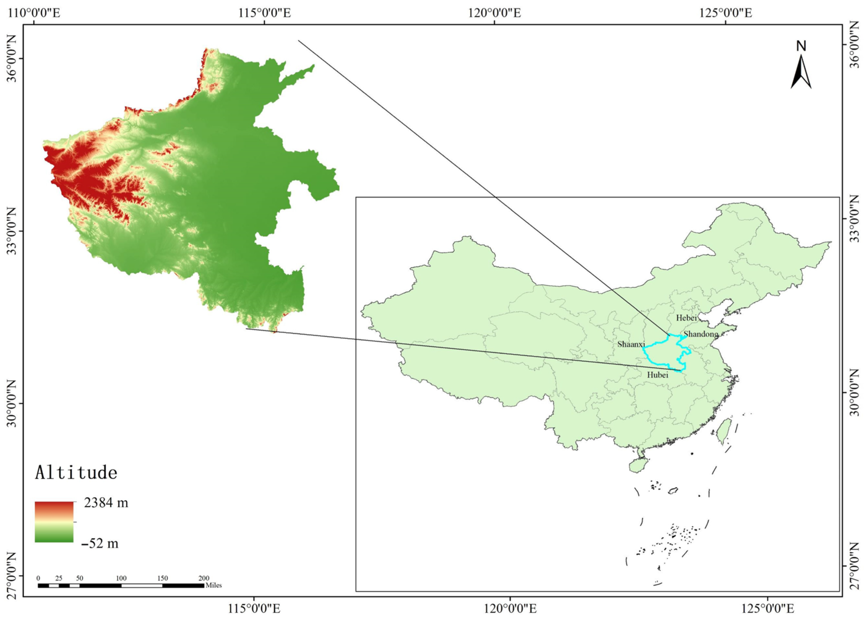
Study Area
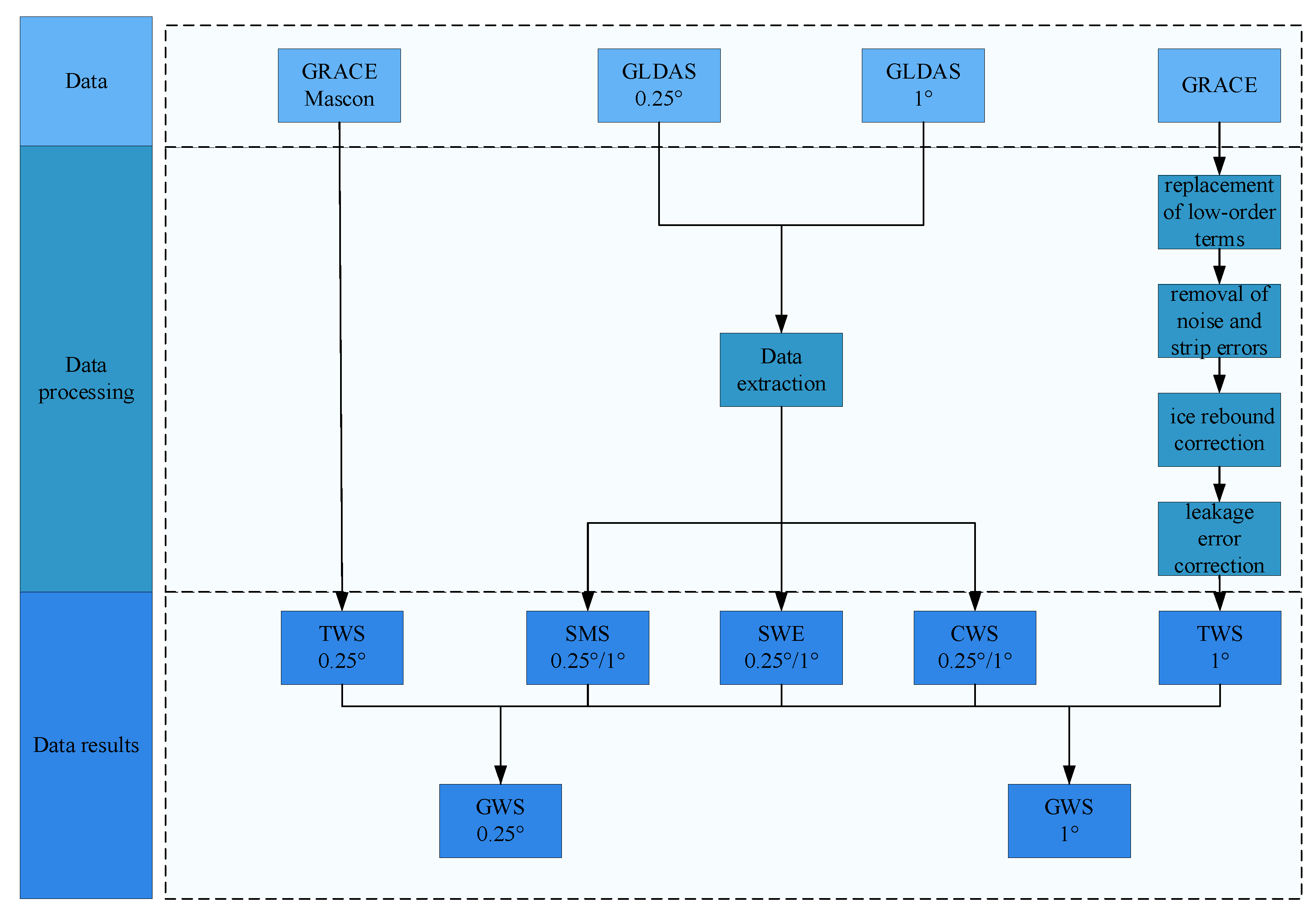
2. Data
2.1. GRACE Satellite Gravity Data
2.2. GLDAS Assimilation Model
2.3. Precipitation Data
3. Methods
3.1. GRACE Inversion of TWS
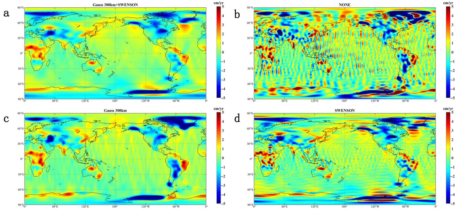
3.2. Gaussian Filtering and Decorrelation Filtering
3.3. Using GLDAS to Monitor TWS and Estimate GWS Changes
3.4. Singular Spectrum Analysis (SSA)
- (1)
- Embedding: The one-dimensional time series data is transformed into a trajectory matrix of size L × K, where L is the window length and K = N − L + 1. The trajectory matrix is defined as follows:
- (2)
- Singular Value Decomposition (SVD): For the matrix , let and denote the eigenvalues and eigenvectors of , respectively, sorted in descending order such that . The corresponding eigenvectors are , , and . Let d = rank(X), the matrix can be decomposed as follows:where , represents the singular spectrum of the sequence X, with the largest singular value corresponding to the eigenvector that captures the dominant trend in the signal. is a column orthogonal matrix.
- (3)
- Grouping: The decomposed components are grouped based on the magnitude of their singular values. By selecting the first r principal components, the reconstructed matrix is as follows:where is matrix with column vectors, called the right singular vectors.
- (4)
- Diagonal Averaging: Converting back into a one-dimensional time series , is realized through the following:where , and denotes the element in the i-th row and j-th column of the matrix .
3.5. Seasonal and Trend Decomposition Using Loess (STL) and Linear Regression
3.6. Conceptual Diagram
4. Results
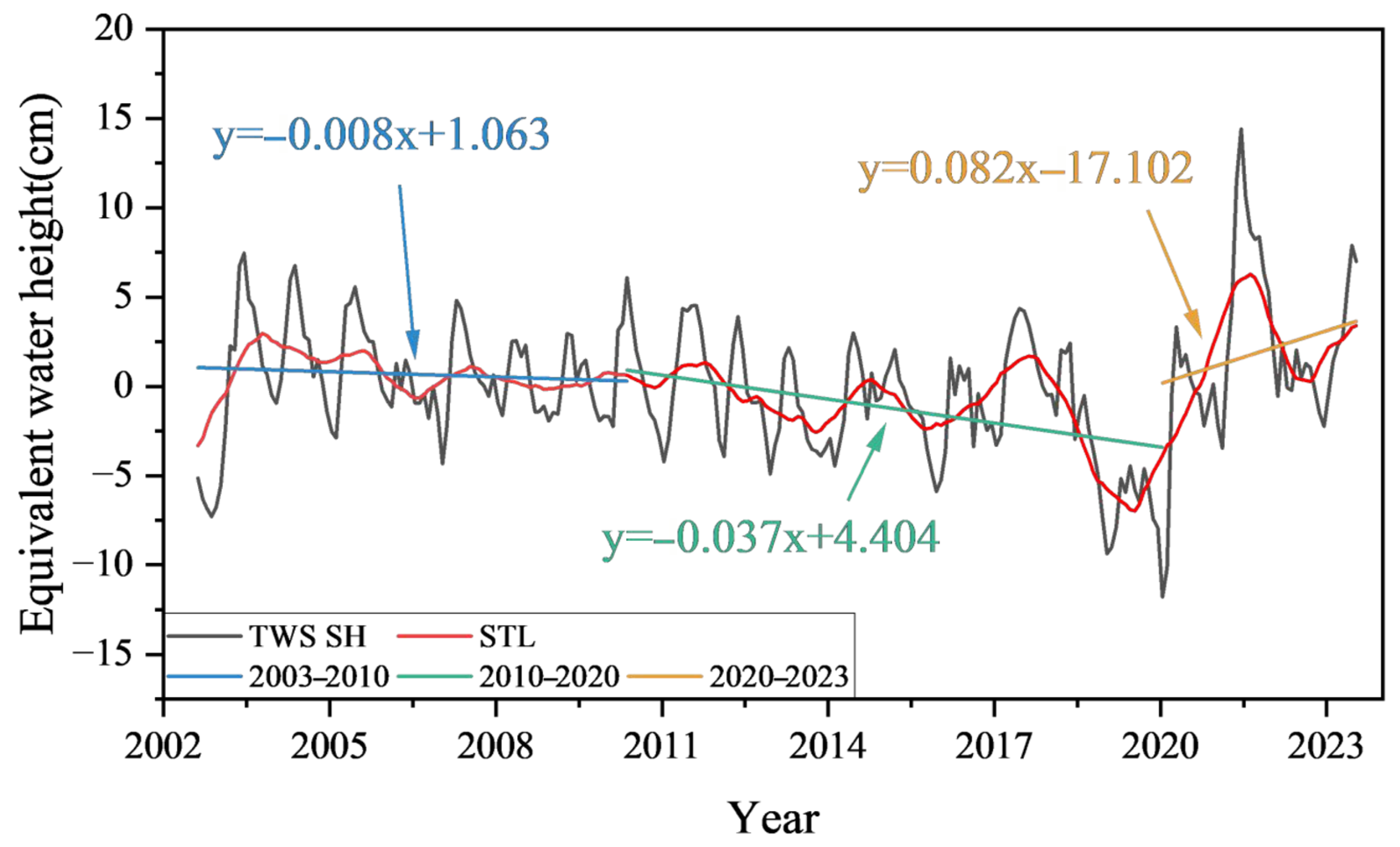
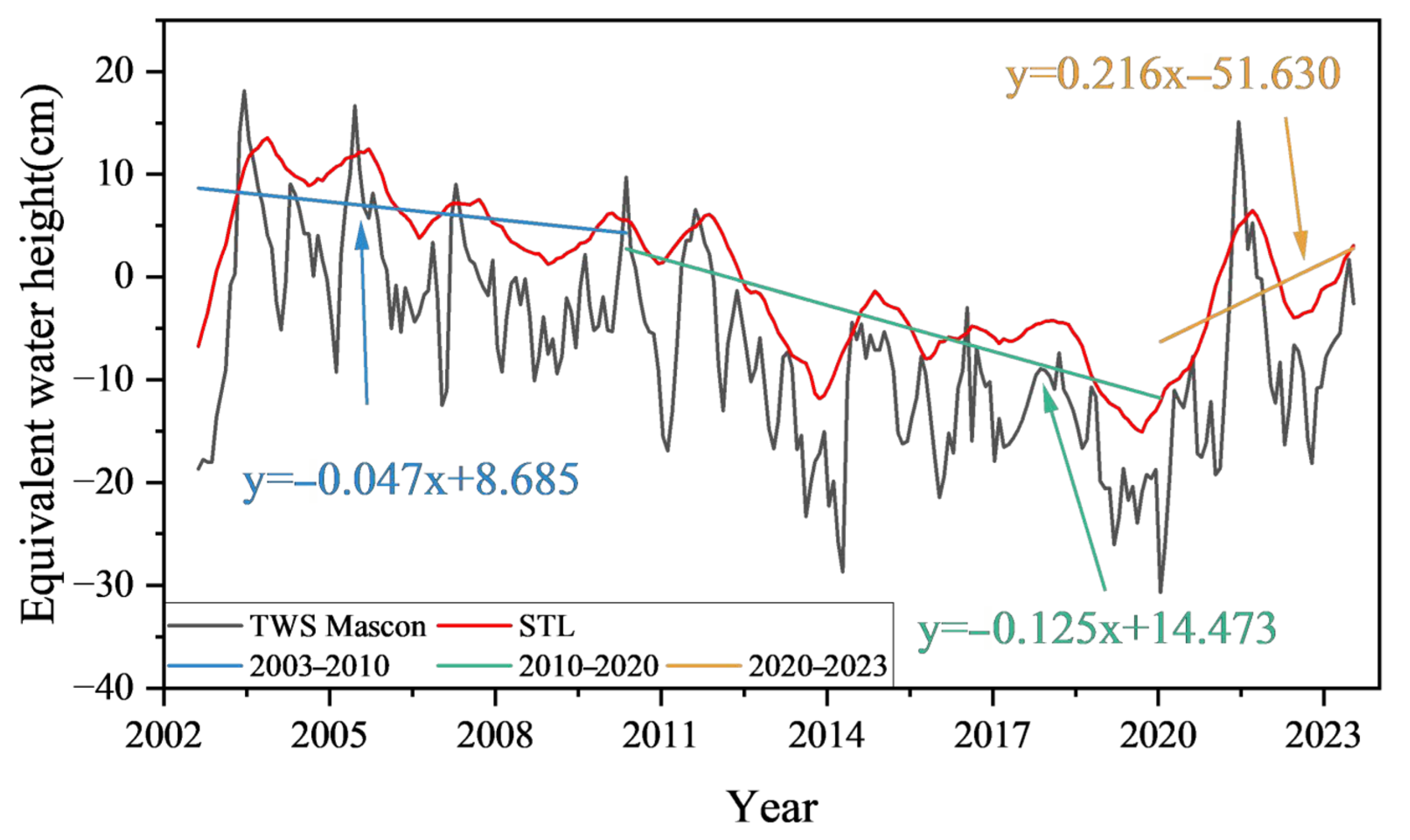
4.1. Time Series Analysis of TWS Variations
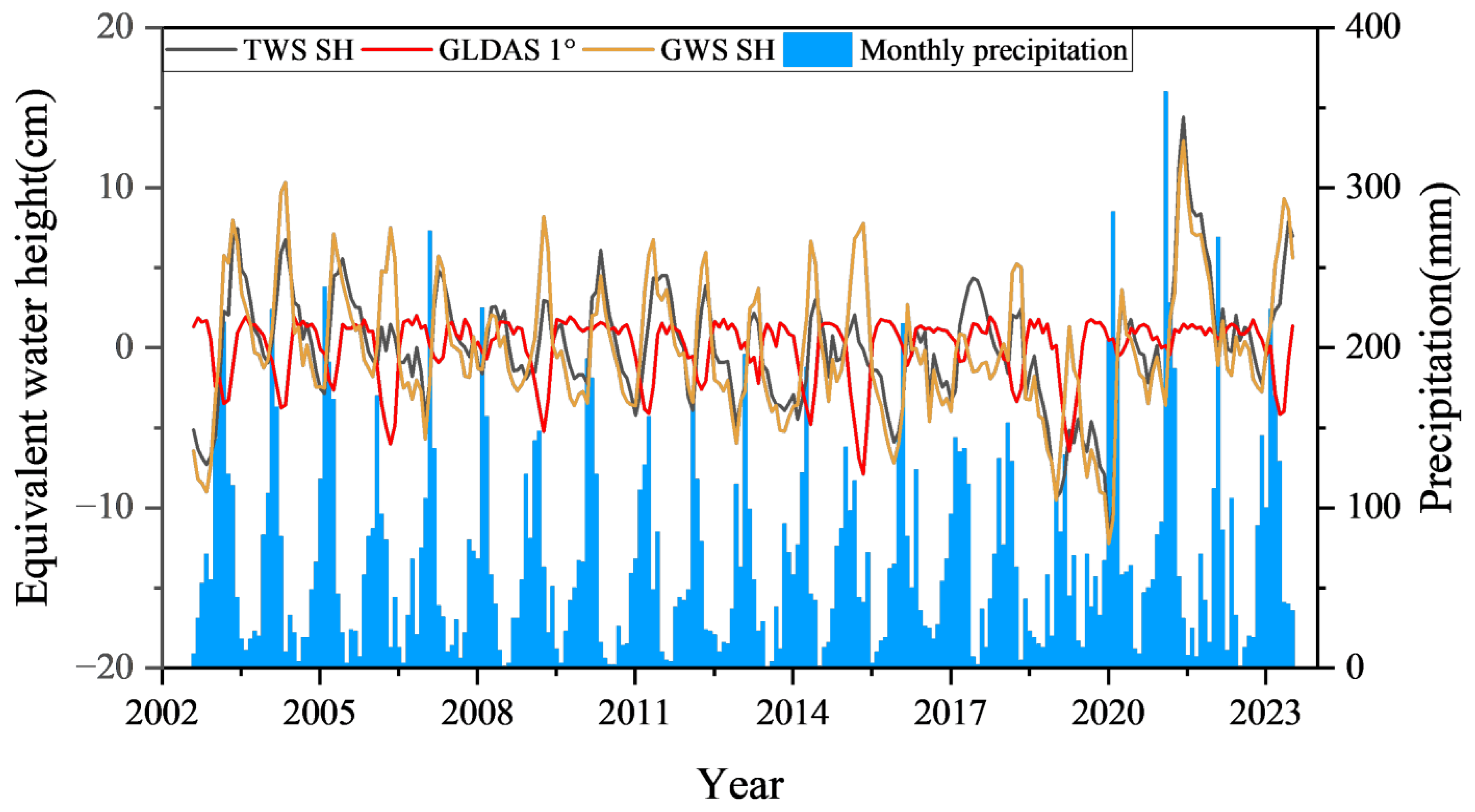
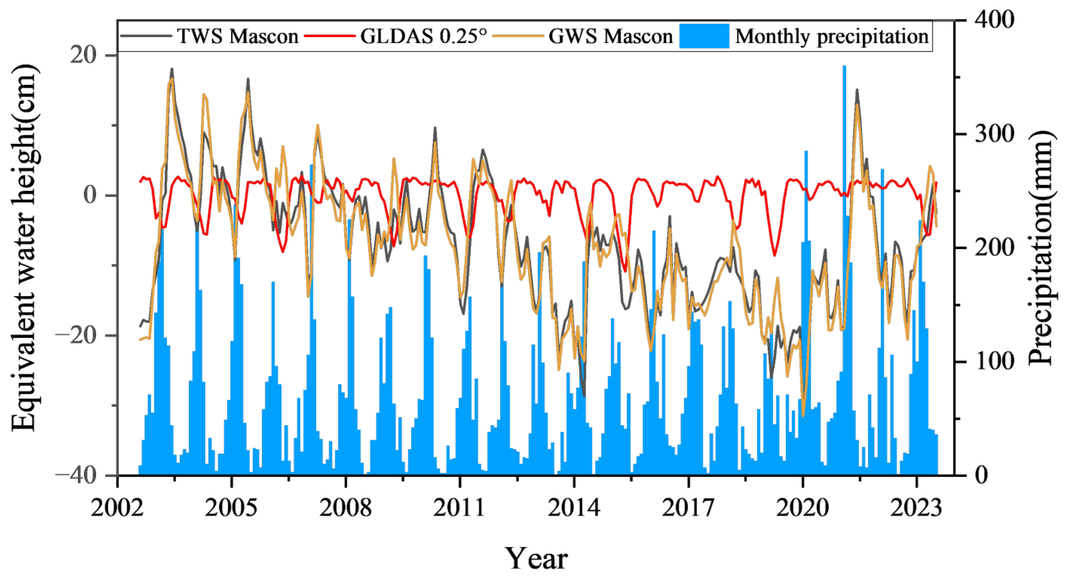
4.2. GRACE and GLDAS Data
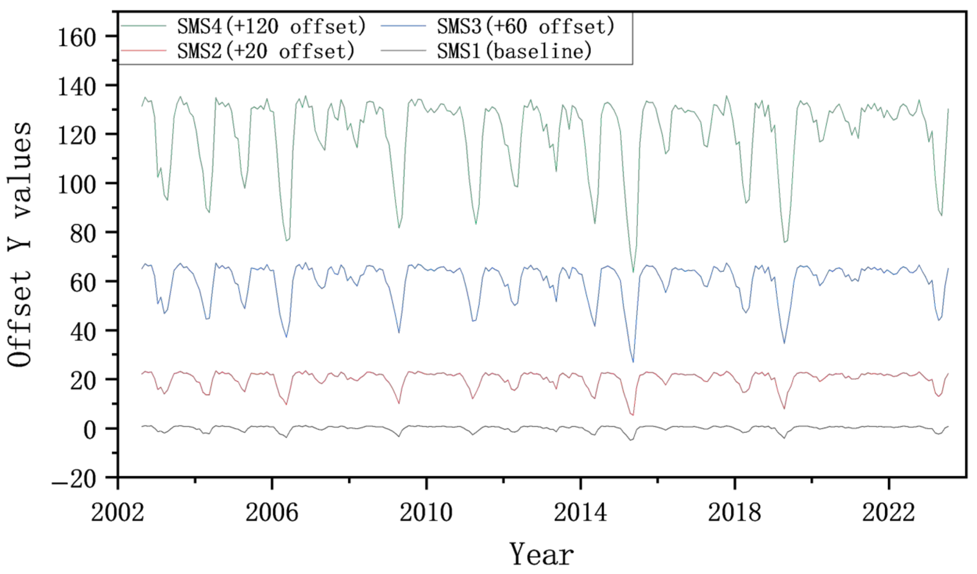
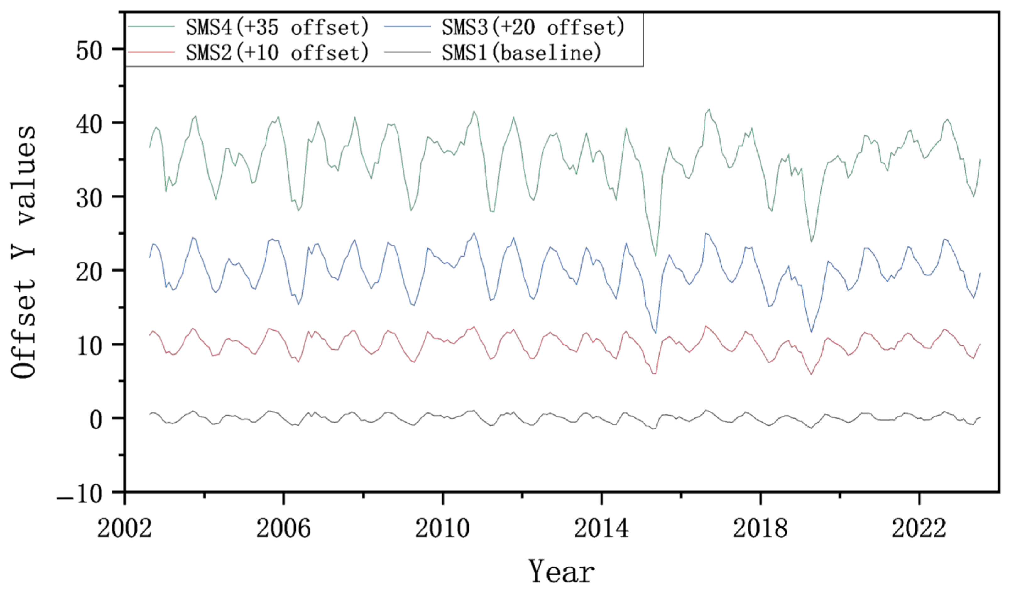
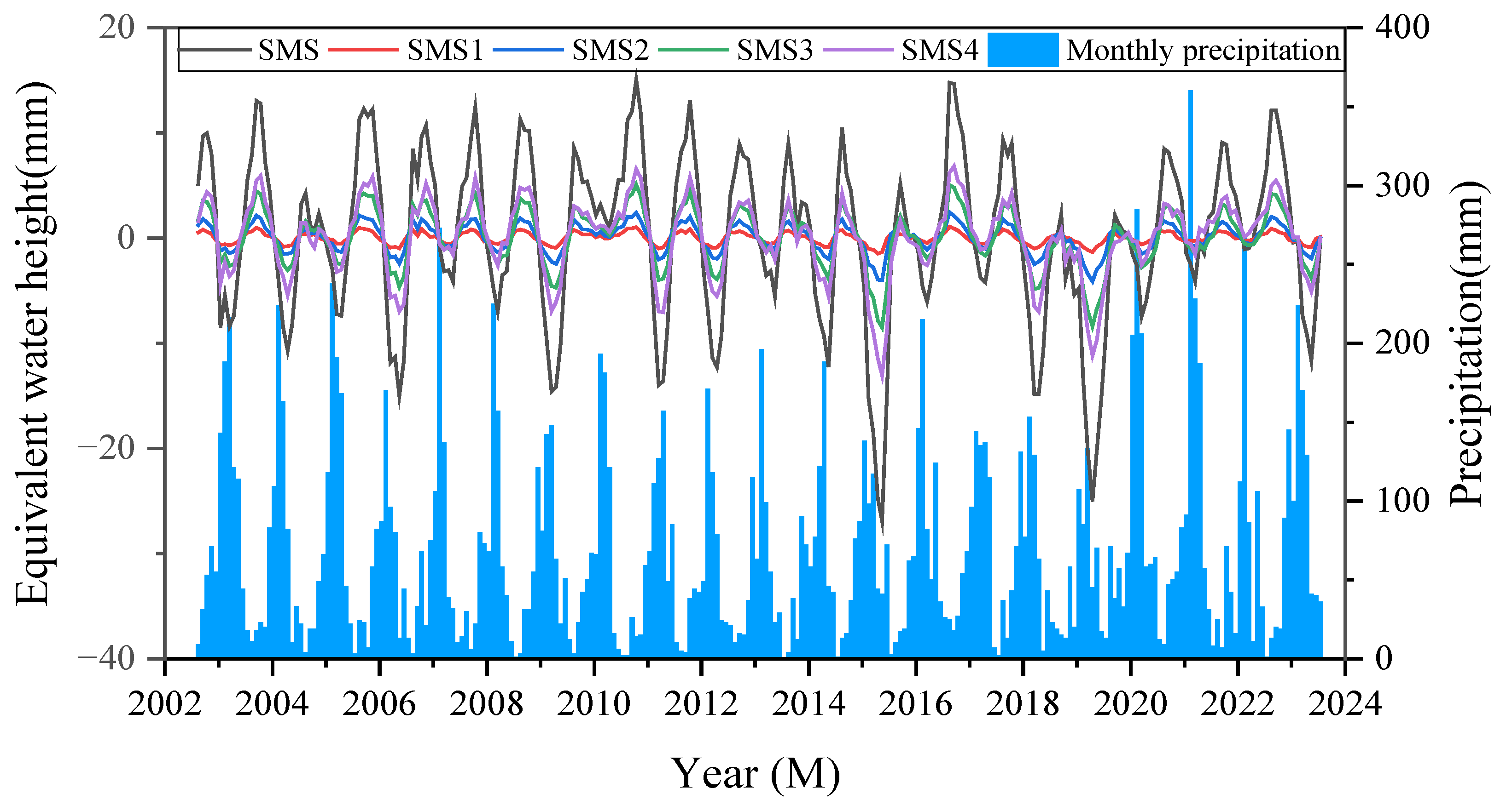
4.3. SMS Data
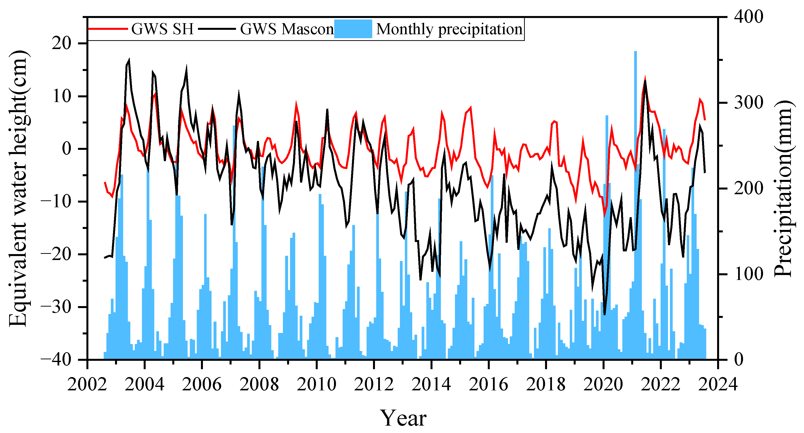
4.4. Time Series Analysis of GWS Variations
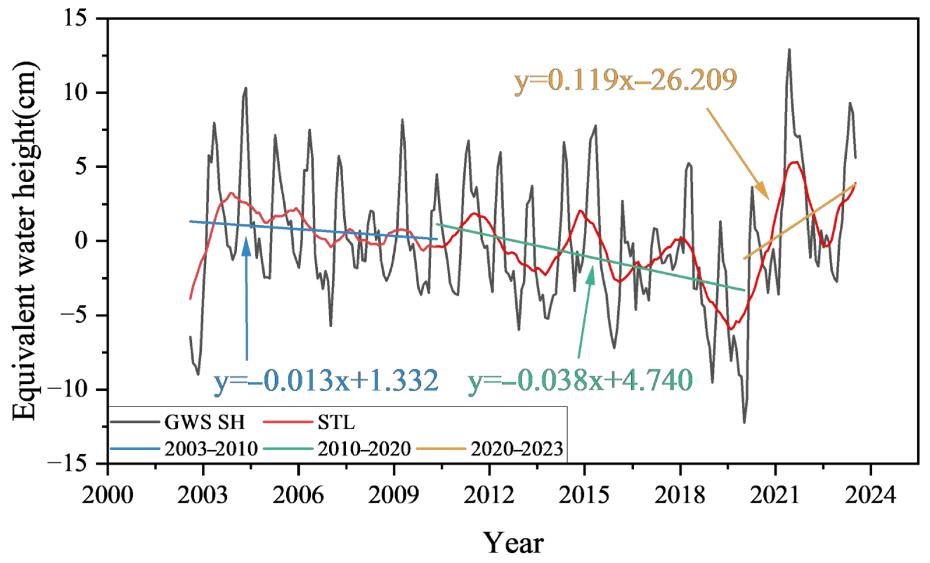
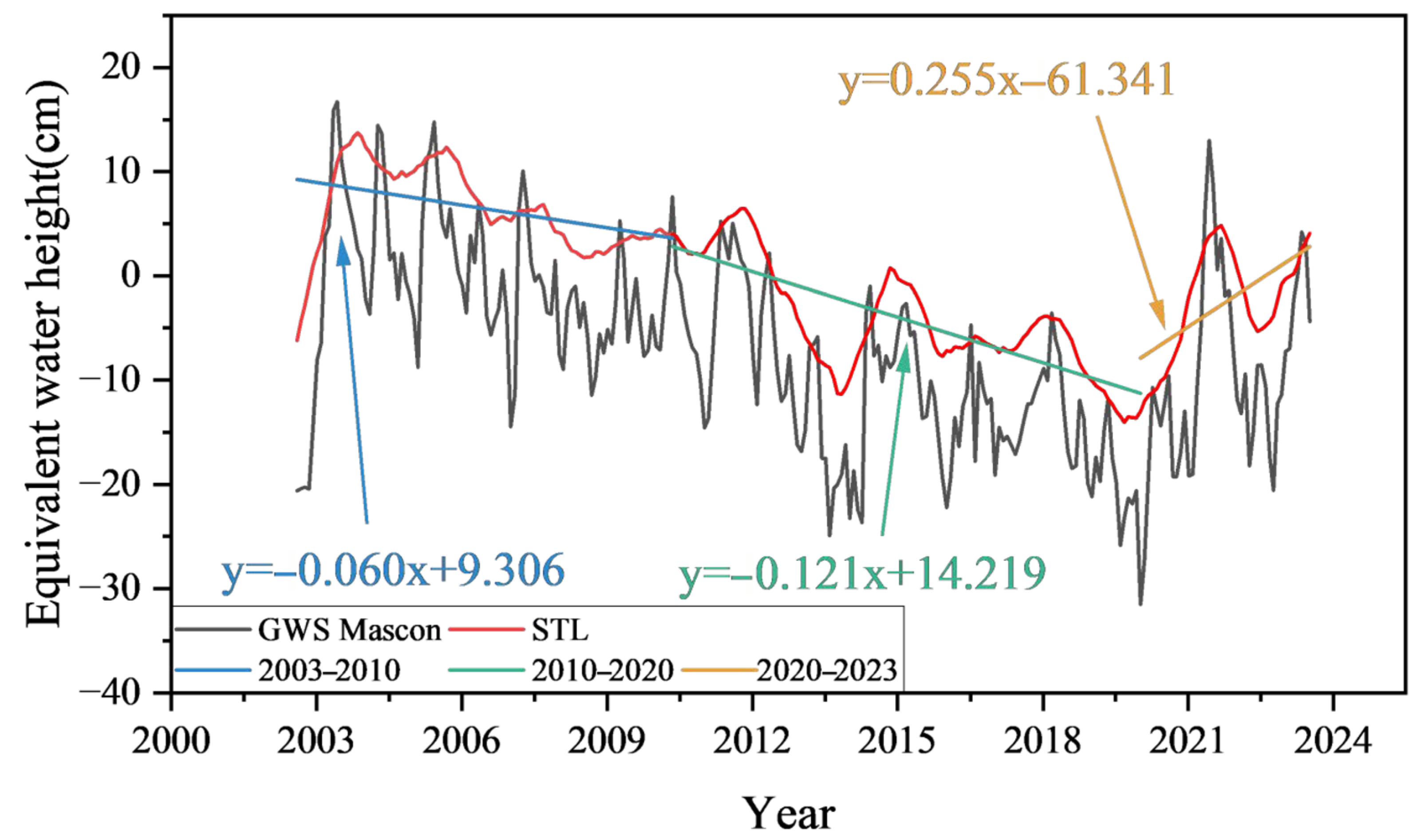
4.5. Rate of Change in TWS and GWS
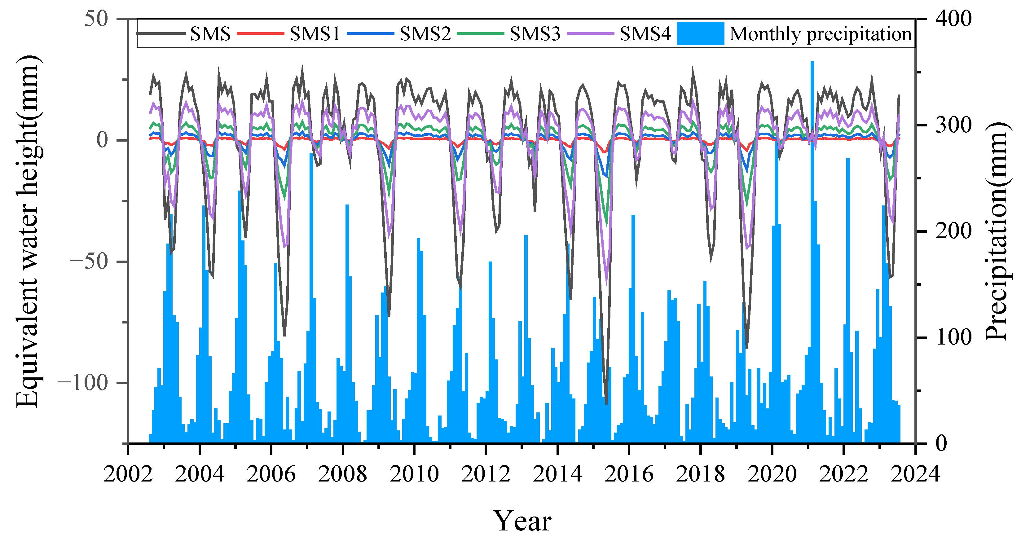
4.6. Comparison Between Rainfall and Individual Data
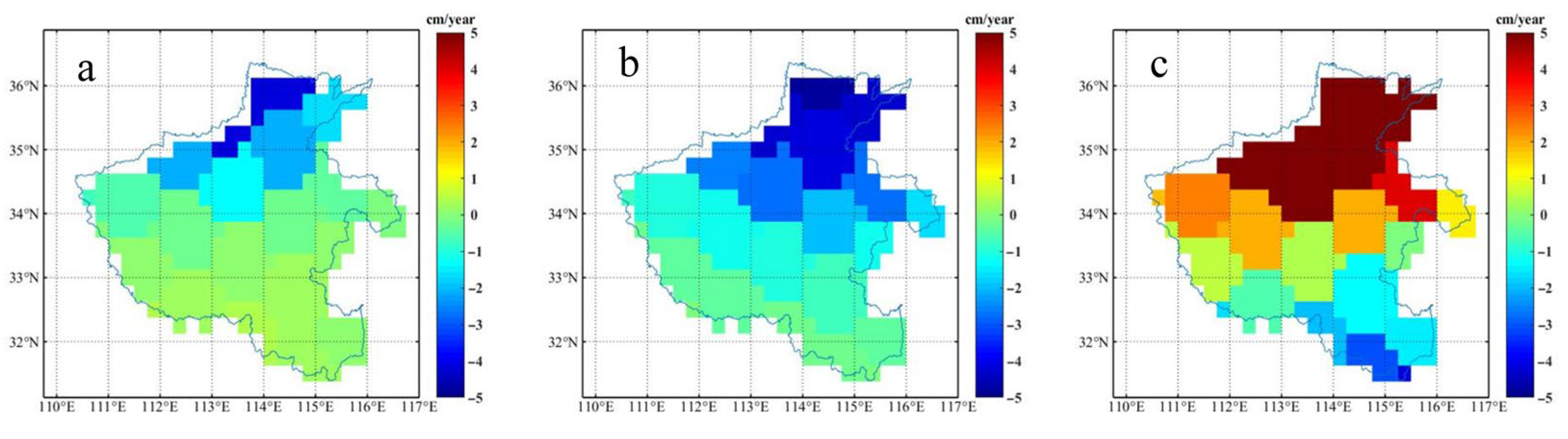
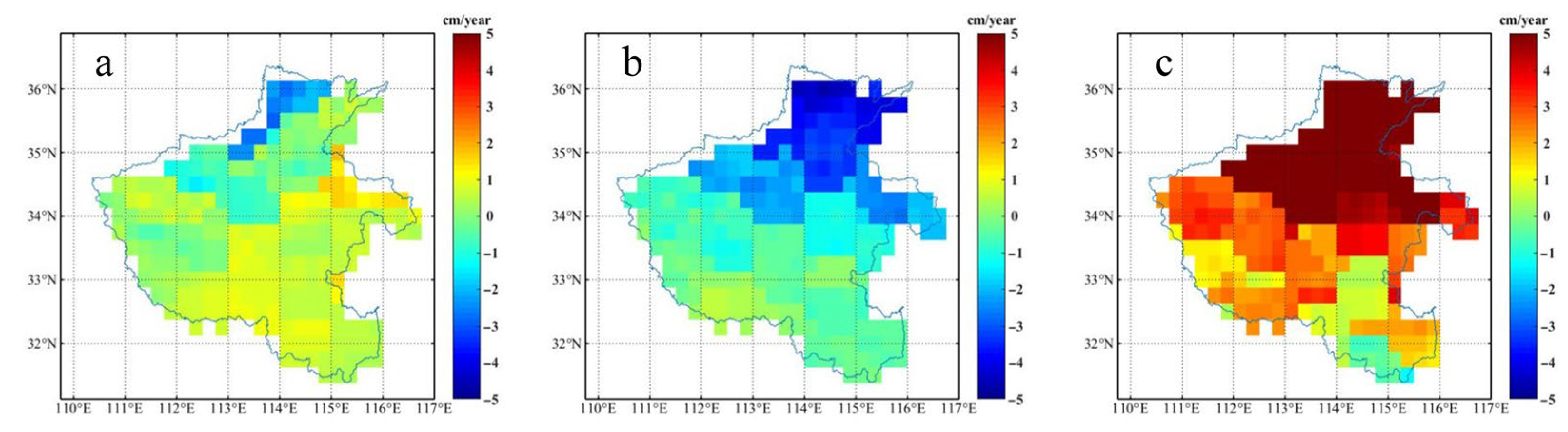
4.7. Spatial Characterization of TWS and GWS Changes
5. Discussion
6. Conclusions
Author Contributions
Funding
Institutional Review Board Statement
Informed Consent Statement
Data Availability Statement
Conflicts of Interest
References
- Li, Q.; Liu, X.; Zhong, Y.; Wang, M.; Zhu, S. Estimation of Terrestrial Water Storage Changes at Small Basin Scales Based on Multi-Source Data. Remote Sens. 2021, 13, 3304. [Google Scholar] [CrossRef]
- Chen, Z.; Zheng, W.; Yin, W.; Li, X.; Zhang, G.; Zhang, J. Improving the Spatial Resolution of GRACE-Derived Terrestrial Water Storage Changes in Small Areas Using the Machine Learning Spatial Downscaling Method. Remote Sens. 2021, 13, 4760. [Google Scholar] [CrossRef]
- Abhishek; Kinouchi, T. Synergetic application of GRACE gravity data, global hydrological model, and in-situ observations to quantify water storage dynamics over Peninsular India during 2002–2017. J. Hydrol. 2021, 596, 126069. [Google Scholar] [CrossRef]
- Sun, W.; Zhang, X. Revealing Water Storage Changes and Ecological Water Conveyance Benefits in the Tarim River Basin over the Past 20 Years Based on GRACE/GRACE-FO. Remote Sens. 2024, 16, 4355. [Google Scholar] [CrossRef]
- Guardiola-Albert, C.; Naranjo-Fernández, N.; Rivera-Rivera, J.S.; Gómez Fontalva, J.M.; Aguilera, H.; Ruiz-Bermudo, F.; Rodríguez-Rodríguez, M. Enhancing groundwater management with GRACE-based groundwater estimates from GLDAS-2.2: A case study of the Almonte-Marismas aquifer, Spain. Hydrogeol. J. 2024, 32, 1833–1852. [Google Scholar] [CrossRef]
- Pang, Y.; Wu, B.; Cao, Y.; Jia, X. Spatiotemporal changes in terrestrial water storage in the Beijing-Tianjin Sandstorm Source Region from GRACE satellites. Int. Soil Water Conserv. Res. 2020, 8, 295–307. [Google Scholar] [CrossRef]
- Deng, S.; Liu, S.; Mo, X. Assessment and attribution of China’s droughts using an integrated drought index derived from GRACE and GRACE-FO data. J. Hydrol. 2021, 603, 127170. [Google Scholar] [CrossRef]
- Jing, W.; Zhao, X.; Yao, L.; Jiang, H.; Xu, J.; Yang, J.; Li, Y. Variations in terrestrial water storage in the Lancang-Mekong river basin from GRACE solutions and land surface model. J. Hydrol. 2020, 580, 124258. [Google Scholar] [CrossRef]
- Xie, J.; Xu, Y.-P.; Wang, Y.; Gu, H.; Wang, F.; Pan, S. Influences of climatic variability and human activities on terrestrial water storage variations across the Yellow River basin in the recent decade. J. Hydrol. 2019, 579, 124218. [Google Scholar] [CrossRef]
- Awange, J.L.; Gebremichael, M.; Forootan, E.; Wakbulcho, G.; Anyah, R.; Ferreira, V.G.; Alemayehu, T. Characterization of Ethiopian mega hydrogeological regimes using GRACE, TRMM and GLDAS datasets. Adv. Water Resour. 2014, 74, 64–78. [Google Scholar] [CrossRef]
- Wei, M.; Zhou, H.; Luo, Z.; Dai, M. Tracking inter-annual terrestrial water storage variations over Lake Baikal basin from GRACE and GRACE Follow-On missions. J. Hydrol. Reg. Stud. 2022, 40, 101004. [Google Scholar] [CrossRef]
- Shamsudduha, M.; Panda, D.K. Spatio-temporal changes in terrestrial water storage in the Himalayan river basins and risks to water security in the region: A review. Int. J. Disaster Risk Reduct. 2019, 35, 101068. [Google Scholar] [CrossRef]
- Ni, S.; Chen, J.; Wilson, C.R.; Li, J.; Hu, X.; Fu, R. Global Terrestrial Water Storage Changes and Connections to ENSO Events. Surv. Geophys. 2017, 39, 1–22. [Google Scholar] [CrossRef]
- Nenweli, R.; Watson, A.; Brookfield, A.; Münch, Z.; Chow, R. Is groundwater running out in the Western Cape, South Africa? Evaluating GRACE data to assess groundwater storage during droughts. J. Hydrol. Reg. Stud. 2024, 52, 101699. [Google Scholar] [CrossRef]
- Hamdi, M.; El Alem, A.; Goita, K. Groundwater Storage Estimation in the Saskatchewan River Basin Using GRACE/GRACE-FO Gravimetric Data and Machine Learning. Atmosphere 2025, 16, 50. [Google Scholar] [CrossRef]
- Rzepecka, Z.; Birylo, M. Groundwater Storage Changes Derived from GRACE and GLDAS on Smaller River Basins—A Case Study in Poland. Geosciences 2020, 10, 124. [Google Scholar] [CrossRef]
- Rzepecka, Z.; Birylo, M.; Jarsjö, J.; Cao, F.; Pietroń, J. Groundwater Storage Variations across Climate Zones from Southern Poland to Arctic Sweden: Comparing GRACE-GLDAS Models with Well Data. Remote Sens. 2024, 16, 2104. [Google Scholar] [CrossRef]
- Sen, S.; Nandi, S.; Biswas, S. Application of GRACE-based satellite estimates in the assessment of flood potential: A case study of Gangetic-Brahmaputra basin, India. Environ. Monit. Assess. 2024, 196, 1–24. [Google Scholar] [CrossRef]
- Jawadi, H.A.; Farahmand, A.; Fensham, R.; Patel, N. Evaluating groundwater storage variations in Afghanistan using GRACE, GLDAS, and in-situ measurements. Model. Earth Syst. Environ. 2024, 10, 5669–5685. [Google Scholar] [CrossRef]
- Zhao, J.; Li, G.; Zhu, Z.; Hao, Y.; Hao, H.; Yao, J.; Bao, T.; Liu, Q.; Yeh, T.-C.J. Analysis of the spatiotemporal variation of groundwater storage in Ordos Basin based on GRACE gravity satellite data. J. Hydrol. 2024, 632, 130931. [Google Scholar] [CrossRef]
- Zhang, J.; Lu, Z.; Li, C.; Lei, G.; Yu, Z.; Li, K. Estimation of groundwater-level changes based on GRACE satellite and GLDAS assimilation data in the Songnen Plain, China. Hydrogeol. J. 2024, 32, 1495–1509. [Google Scholar] [CrossRef]
- Mohasseb, H.A.; Shen, W.; Abd-Elmotaal, H.A.; Jiao, J. Assessing Groundwater Sustainability in the Arabian Peninsula and Its Impact on Gravity Fields through Gravity Recovery and Climate Experiment Measurements. Remote Sens. 2024, 16, 1381. [Google Scholar] [CrossRef]
- Li, W.; Zhang, C.; Wang, W.; Guo, J.; Shen, Y.; Wang, Z.; Bi, J.; Guo, Q.; Zhong, Y.; Li, W.; et al. Inversion of Regional Groundwater Storage Changes Based on the Fusion of GNSS and GRACE Data: A Case Study of Shaanxi–Gansu–Ningxia. Remote Sens. 2023, 15, 520. [Google Scholar] [CrossRef]
- Shen, Y.; Zheng, W.; Zhu, H.; Yin, W.; Xu, A.; Pan, F.; Wang, Q.; Zhao, Y. Inverted Algorithm of Groundwater Storage Anomalies by Combining the GNSS, GRACE/GRACE-FO, and GLDAS: A Case Study in the North China Plain. Remote Sens. 2022, 14, 5683. [Google Scholar] [CrossRef]
- Xue, H.; Zhang, R.; Luan, W.; Yuan, Z. The Spatiotemporal Variations in and Propagation of Meteorological, Agricultural, and Groundwater Droughts in Henan Province, China. Agriculture 2024, 14, 1840. [Google Scholar] [CrossRef]
- Hu, J.; Zhou, Z.; Wang, J.; Qin, F.; Wang, J.; Zhang, R.; Wang, L.; Wu, W.; Huang, L. Enhancing the groundwater storage estimates by integrating MT-InSAR, GRACE/GRACE-FO, and hydraulic head measurements in Henan Plain (China). Int. J. Appl. Earth Obs. Geoinf. 2024, 131, 103993. [Google Scholar] [CrossRef]
- Wahab, F.A.J.A.; Al-Abadi, A.M.; Al-Ozeer, A.Z.A. Groundwater depletion and annual groundwater recharge estimation in Nineveh Plain, Northern Iraq using GRACE, GLDAS, and field data. Model. Earth Syst. Environ. 2025, 11, 1–19. [Google Scholar] [CrossRef]
- Wahr, J.; Molenaar, M.; Bryan, F. Time variability of the Earth’s gravity field: Hydrological and oceanic effects and their possible detection using GRACE. J. Geophys. Res. Solid Earth 1998, 103, 30205–30229. [Google Scholar] [CrossRef]
- Swenson, S.; Wahr, J. Post-processing removal of correlated errors in GRACE data. Geophys. Res. Lett. 2006, 33, L08402. [Google Scholar] [CrossRef]
- Jin, S.; Feng, G. Large-scale variations of global groundwater from satellite gravimetry and hydrological models, 2002–2012. Glob. Planet. Change 2013, 106, 20–30. [Google Scholar] [CrossRef]
- Shuang, Y.; Nico, S. Filling the Data Gaps Within GRACE Missions Using Singular Spectrum Analysis. J. Geophys. Res. Solid Earth 2021, 126, e2020JB021227. [Google Scholar]
- Arega, K.A.; Birhanu, B.; Ali, S.; Hailu, B.T.; Tariq, M.A.U.R.; Adane, Z.; Nedaw, D. Analysis of spatio-temporal variability of groundwater storage in Ethiopia using Gravity Recovery and Climate Experiment (GRACE) data. Environ. Earth Sci. 2024, 83, 206. [Google Scholar] [CrossRef]
- Ding, K.; Zhao, X.; Cheng, J.; Yu, Y.; Luo, Y.; Couchot, J.; Zheng, K.; Lin, Y.; Wang, Y. GRACE/ML-based analysis of the spatiotemporal variations of groundwater storage in Africa. J. Hydrol. 2025, 647, 132336. [Google Scholar] [CrossRef]
- Hua, S.; Jing, H.; Qiu, G.; Kuang, X.; Andrews, C.B.; Chen, X.; Zheng, C. Long-term trends in human-induced water storage changes for China detected from GRACE data. J. Environ. Manag. 2024, 368, 122253. [Google Scholar] [CrossRef]
- Zhang, K.; Xie, X.; Zhu, B. Water storage and vegetation changes in response to the 2009/10 drought over North China. Hydrol. Res. 2018, 49, 1618–1635. [Google Scholar] [CrossRef]
- Yan, X.; Zhang, B.; Yao, Y.; Yang, Y.; Li, J.; Ran, Q. GRACE and land surface models reveal severe drought in eastern China in 2019. J. Hydrol. 2021, 601, 126640. [Google Scholar] [CrossRef]
- Xiao, C.; Zhong, Y.; Feng, W.; Gao, W.; Wang, Z.; Zhong, M.; Ji, B. Monitoring the Catastrophic Flood With GRACE-FO and Near-Real-Time Precipitation Data in Northern Henan Province of China in July 2021. IEEE J. Sel. Top. Appl. Earth Obs. Remote Sens. 2023, 16, 89–101. [Google Scholar] [CrossRef]

| CSR Data | Spatial Resolution | Time Resolution |
|---|---|---|
| CSR SH | 1° | Monthly scale |
| CSR Mascon | 0.25° | Monthly scale |
| Property Abbreviation | Property Name | Unit | Spatial Resolution | Temporal Resolution | |
|---|---|---|---|---|---|
| CWS | Total canopy water storage | kg/m2 | 0.25°/1° | Monthly | |
| SWE | Snow water equivalent | kg/m2 | 0.25°/1° | Monthly | |
| SMS | SMS1 | 0~10 cm average layer 1 soil moisture | kg/m2 | 0.25°/1° | Monthly |
| SMS2 | 10~40 cm average layer 2 soil moisture | ||||
| SMS3 | 40~100 cm average layer 3 soil moisture | ||||
| SMS4 | 100~200 cm average layer 4 soil moisture | ||||
| TWS SH Rate(cm/year) | Confidence Interval | GWS SH Rate (cm/year) | Confidence Interval | TWS Mascon Rate (cm/year) | Confidence Interval | GWS Mascon Rate (cm/year) | Confidence Interval | |
|---|---|---|---|---|---|---|---|---|
| 2003.01–2010.10 | 1.47 | [−2.95, 5.84] | 1.45 | [−4.62, 7.45] | 3.85 | [−7.60, 14.93] | 3.78 | [−8.64, 15.91] |
| 2010.10–2020.06 | −1.57 | [−5.83, 2.13] | −1.47 | [−7.12, 3.65] | −3.47 | [−13.69, 5.34] | −3.37 | [−14.09, 6.00] |
| 2020.06–2023.12 | 4.16 | [−4.83, 15.55] | 4.11 | [−5.72, 15.92] | 4.51 | [−10.90, 26.95] | 4.51 | [−12.07, 27.56] |
Disclaimer/Publisher’s Note: The statements, opinions and data contained in all publications are solely those of the individual author(s) and contributor(s) and not of MDPI and/or the editor(s). MDPI and/or the editor(s) disclaim responsibility for any injury to people or property resulting from any ideas, methods, instructions or products referred to in the content. |
© 2025 by the authors. Licensee MDPI, Basel, Switzerland. This article is an open access article distributed under the terms and conditions of the Creative Commons Attribution (CC BY) license (https://creativecommons.org/licenses/by/4.0/).
Share and Cite
Xu, H.; Liu, D. Study on Groundwater Storage Changes in Henan Province Based on GRACE and GLDAS. Sustainability 2025, 17, 6316. https://doi.org/10.3390/su17146316
Xu H, Liu D. Study on Groundwater Storage Changes in Henan Province Based on GRACE and GLDAS. Sustainability. 2025; 17(14):6316. https://doi.org/10.3390/su17146316
Chicago/Turabian StyleXu, Haijun, and Dongpeng Liu. 2025. "Study on Groundwater Storage Changes in Henan Province Based on GRACE and GLDAS" Sustainability 17, no. 14: 6316. https://doi.org/10.3390/su17146316
APA StyleXu, H., & Liu, D. (2025). Study on Groundwater Storage Changes in Henan Province Based on GRACE and GLDAS. Sustainability, 17(14), 6316. https://doi.org/10.3390/su17146316